
Document
Ben-Gurion Universityy of the Negev Beng Department of Chemistry MOLECULAR MAGNETISM AND MATERIALSMATERIALSTHEORY AND APPLICATIONS Professor Boris Tsukerblat [email protected] @ g Beer--Sheva Beer 2006 SYLLABUS I. Scope of molecular magnetism. Diversity of the field. Main kinds of magnetic systems and the main types of the magnetic ti ordering. d i II. Spin, fundamental equations in molecular magnetism. Magnetic susceptibility , magnetic moments moments. Curie-Weiss low low, magnetization. Electron paramagnetic resonance. III. Magnetic properties of a free ion, molecules containing a unique i magnetic ti center t without ith t first-order fi t d orbital bit l magnetism ti and EPR of transition metal ions and rare-earths, spin-orbital interaction. IV. Effects of crystal field. Group-theoretical introduction. Ground terms of the transition metal ions in the crystal fields. Anisotropy py of the g g-factor. Zero-field splitting: p g q qualitative and quantitative approaches. Covalence and orbital reduction. EPR of the metal ions in complexes. V. Exchange interaction in clusters. Exchange effect, the nature of the potential exchange. Magnetic properties of binuclear compounds, dimers of Cu(II) , EPR, magnetic anisotropy. VI Heisenberg-Dirac-Van VI. Heisenberg Dirac Van Vleck model of the exchange interaction. Concept of spin-Hamiltonian. Many-electron problem of the exchange. Spin-coupling scheme for the polynuclear compounds compounds, Kambe’s Kambe s approach. approach Trimeric and tetrameric clusters: basic chromium and iron acetates. EPR spectra of polynuclear compounds. VII Single VII. Si l molecule l l magnets, physical h i l principlesi i l quantum tunneling, relaxation. Mn12-ac molecule. Applications in molecule-based devices. VIII. Mixed-valence compounds. The phenomenon of mixed valence. Spin-dependent delocalization-double exchange- classical and quantum-mechanical exchange quantum mechanical description (Anderson’s theory). Robin and Day classification of mixed-valence compounds. Intervalence light absorption (light induced electron transfer) transfer). Magnetic properties. SOURCES SOURCES: 1) CD D (Power Point file) 2)THE MAIN BOOKS AND 3) REFERENCES THROUGHOUT THE FILE • • • • • Oliver Kahn Kahn, Molecular Magnetism Magnetism, VCH,NY(1993). VCH NY(1993) Alessandro Bencini, Dante Gatteschi, Electron Paramagnetic Resonance of Exchange Coupled Systems, Springer-Verlag, Berlin (1990) (1990). F.A.Cotton, Chemical Application of Group Theory, 2nd Edition, Interscience, New York (1971). B.S.Tsukerblat, Group Theory in Chemistry and Spectroscopy. A Simple Guide to Advanced Usage, Academic Press, London (1994). J.J.Borras-Almenar, J.M.Clemente-Juan, E.Coronado, A.V.Palii, B.S.Tsukerblat, Magnetic Properties of Mixed-Valence Clusters:Theoretical Approaches and Applications, in: “M “Magnetism: ti Molecules M l l tto M Materials”, t i l ” ( J.Miller, M.Drillon, Eds.), Wiley-VCH (2001) p.p.155-210. ABOUT THE BOOKS BOOKS--MOLECULAR MAGNETISM Chapter 5 ABOUT THE BOOKS BOOKS--GROUP THEORY Exceptionally clear presentation ! YOU ARE EXPECTED TO KNOW: • • • • Main concept of quantum mechanics: Schrödinger equation, wave-functions, f hydrogen atom, many-electron atoms, some knowledge of the perturbation theory. Orbital and spin p angular g momenta. Pauli p principle. p Group theory for chemists (standard course for chemists): how to determine the point symmetry group that the molecule belongs to to, concept of the reducible and irreducible representations, classification of the molecular energy levels, selection rules. Classification of molecular vibrations. vibrations Background of the crystal field theory for transition metal ions: general idea of the crystal field splitting and some results for the transition and rare rare-earth earth ions ions. Molecular orbital approach – the main concepts. YOU ARE EXPECTED TO LEARN • Magnetic substances. substances. The main kinds of magnetic behavior. Basic concepts: p magnetic g moments,, magnetic g susceptibility. Spin, free ions, spin-orbit coupling, g-factors. Electron paramagnetic resonance. • Crystal C t l fifield ld th theory role theory, l off the th ligands, li d magnetic ti properties of complex compounds, zero-field splitting, g resonance,, anisotropy py of g g-factors. magnetic • Exchange interaction in clusters. Properties of polunuclear compounds. Magnetic anisotropy, nanoscience i -single i l molecular l l magnets. t • Concept of mixedmixed-valency and electron transfer double exchange ferromagnetic effect of the double exchange, exchange, exchange role of the electron-vibrational interactions-localization vs. delocalization. Spin-dependent delocalzation in ironsulphur l h proteins. t i LIST OF THE MAIN NOTATIONS (to be used as necessary) • H - magnetic field (vector), H - magnetic field - absolute value (font --" arial arial" ). ) • Vectors and matrices – bold. • Hˆ Hamiltonia H ilt i n (font (f t - " times ti new Roman, R It li " ). Italic" ) • Operators are marked by " cap" : Hˆ , etc . • S - spin (quantum number), S - classical spin vector, Sˆ spin p operator p ((vector operator p - bold and " cap" p ), Sˆ x , Sˆ y , Sˆ z components of the vector operator Sˆ . • L - quantum number of the orbital angular momentum, momentum ˆ operator (vector operator). L - classical vector, L ˆ. Lˆx , Lˆ y , Lˆz components of the vector operator L • J - quantum number of the total angular momentum, J - classical vector, ector Jˆ operator (vector ( ector operator), operator) Jˆ x , Jˆ y , Jˆ z components of the vector operator Jˆ . • M S , M L , M J ,- magnetic quantum numbers of spin, orbital angular momentum and total angular momentum. • g e g factor of a free electron, g J g factor of a LSJ state. • - magnetic susceptibi lity. • μ magnetic g moment ((classical vector), ), ˆ magnetic moment (vector operator), • μ magnetic moment (absolute value) • Hˆ ZFS zero field splitting Hamiltonia n. • D zero - field splitting parameter. parameter • J exchange parameter Chapter p I Scope of molecular magnetism. Diversity of the field. The main kinds of magnetic systems and the main types of the magnetic ordering SCOPE OF MOLECULAR MAGNETISM ♠ Magnetic properties of isolated atoms ,ions ions and molecules ( in particular, metal complexes) containing one magnetic g center. Example: complex ion –coordination compound Metal--(Ligand) Metal ( g )6 NH3 NH3 NH3 Cr NH3 NH3 NH3 [Cr (NH3)6]3+ or [Cr(NH3)6]Cl3 Central metal ion ion- Cr3+ surrounded by six ammonia molecules, Cr3+ contains three unpaired d-electrons Octahedral symmetry, Oh point group ♠ Magnetic properties of the molecules containing more than one magnetic centers – polynuclear compounds, magnetic clusters or exchange clusters. Example: binuclear Co cluster, bi-octahedral edgeshared geometry- oxygen bridged system NH3 NH3 NH3 OH Co NH3 Co OH NH3 NH3 NH3 [(H3N)4Co(OH)2Co(NH3)4]4+ NH3 Co2+(d7-shell)C h ll) bearer of magnetism Point symmetry D2h POLYOXOANION [Ni3 Na(H2O)2(AsW9O34]11WO6 NiO6 3Ni2+magnetic g fragment Na AsO4 Polyhedral representation Ball and stick representation Inorg. Chem. ,2003, 42, 5143-52 POLYOXOANION [Ni6 As3W24O94(H2O)17]- Two 3Ni2+T magnetic f fragments t WO6 NiO6 AsO4 P l h d l representation Polyhedral t ti B ll and Ball d stick ti k representation t ti Inorg. Chem. ,2003, 42, 5143-52 ♠ Assemblies of molecules with the magnetic interactions b t between th the molecular l l entities, titi one-dimensional di i l systems t Structure of donor-acceptor compound (TTF)+[CuS4C4(CF3)4]with TTF+= tetrathiafulvalinium. Phys.Rev.Lett.,35(1975) 744 Structure of the ferrimagnetic chain MnCu(pba)(H2O)3·2(H2O) with pba= b 1,3-propilene-bis(oxamato). 13 il bi ( ) Inorg.Chem.,26(1987)138. DIVERSITY OF THE FIELD,SELECTED APPLICATIONS L N Material sciences Biology Molecular magnetism Molecular M l l electronics NanoN Nanoscience SINGLE MOLECULAR MAGNETMAGNETMAGNET IN ONE MOLECULE [Mn12O12 (CH3COO)16 (H2O)4] -molecule - Mn12-ac (Mn12-acetate) Molecular electronics NanoNanoscience i Mn4+ Mn 3+ MANGANESE--12 CLUSTER MANGANESE eight Mn3+ ions (Si =2) and four Mn4+(Si =3/2) PHYSICAL BACKGROUND – BRIEFLY Pictures: Michel Verdaguer z Thermal activation E y x En nergy 0 2 DS z DS2 - Sz Magnetization vectors -4 -2 0 +2 +4 Direction of magnetization Sz +Sz Barrier for anisotropy If tthe e Mn12-ac ac molecule o ecu e is s magnetized ag et ed by a an app applied ed field, the molecule retains magnetization for a long time , approximately 108 seconds = 3 years at 1.5K A li ti Applications: quantum computing , memory storage elements in one molecule MULTIFUNCTIONAL MATERIALS Molecular electronics Material sciences Nature 408, 421 - 422 (2000) Molecular electronics: A dual dual-action action material FERNA NDO PALACIO* AND JOE L S. MILLE R Fernando Palacio is at the Instituto de Ciencia de Materiales de Aragón, CSIC, Universidad de Zaragoza, 50009 Zaragoza, Spain. e-mail: [email protected] Joel S. Miller is in the Department of Chemistry, University of Utah, Salt Lake City, Utah 841120850, USA. e-mail: [email protected] In the drive for smaller electronic components, chemists are thinking on a molecular l l scale. l By B combining bi i two simple i l molecules, l l a hybrid h b id has h been b produced d d that is both magnetic and an electrical conductor. DISCOVERY OF MULTIFUNCTIONAL MOLECULE--BASED MATERIALS MOLECULE Nature 408, 447 - 449 (2000) Coexistence of ferromagnetism and metallic conductivity in a molecule-based layered compound EUGENIO CORONADO*, JOSÉ É R. GALÁN-MASCARÓS*†, Á Ó CARLOS J. GÓME Ó Z-GA RCÍA* Í & VLADIMIR LAUKHIN*† * Instituto de Ciencia Molecular, Universidad de Valenc ia, Dr. Moliner 50, 46100 Bur jjasot, Spain p † Present addresses: Department of Chemistry, Texas A&M University, College Station, Texas, USA (J.R.G.- M.); ICMBCSIC, Campus de la UAB, 08193 Bellaterra, Spain (V.L.) Crystal engineering engineering—the the planning and construction of crystalline supramolecular architectures from modular building blocks—permits the rational design of functional molecular materials that exhibit technologically useful behavior such as conductivity and superconductivity, superconductivity ferromagnetism and nonlinear optical properties. properties Because the presence of two cooperative properties in the same crystal lattice might result in new physical phenomena and novel applications, a particularly attractive goal is the design of molecular materials with two properties that are difficult or impossible to combine in a conventional inorganic solid with a continuous lattice. A DUAL ACTION MATERIAL Molecular components: ( ) The (a) organic molecule BEDT TTF BEDT-TTF bis(ethylenedithio) tetrathiafulvalene (b) A ferromagnetic bimetallic complex of manganese(ii)tris(oxalato)chromium(iii). Carbon atoms are in p pink, sulphur p in blue. By alternating layers of the molecules in a and b, E. Coronado et al. (Nature) have created a hybrid material that supports both magnetism and conduction. M- magnetic layers, E-conducting layers Structures of the hybrid material and the two sublattices. sublattices a, View of the [MIIMIII(C2O4)3]- bimetallic layers. Filled and open circles in the vertices of the hexagons represent the two types of metals. b Structure b, St t off the th organic i layer, l showing h i the th packing ki off th the BEDT BEDT-TTF TTF molecules. l l c, Representation of the hybrid structure along the c axis, showing the alternating organic/inorganic layers. BIOLOGICAL SYSTEMSSYSTEMS-TWO EXAMPLES Tri--iron cluster Tri Di--iron cluster Di S-cys S Fe Schematic structure of the protein with [Fe3S4] core. core S-cys stands for the sulfur atom of a cystein group. Th Three magnetically ti ll coupled l dF Fe iions. Schematic structure of the two iron (Fe2+, Fe3+ ) ferredoxin two-iron ferredoxin. S-cys stands for the sulfur atom of a cystein group. T Two magnetically ti ll coupled l dF Fe iions. MAIN KINDS OF MAGNETIC SUBSTANCES paramagnet ferromagnet antiferromagnet Disordered directions of the magnetic moments,, macroscopic magnetization is zero Long-range collinear alignment of all moments in the substance, spontaneous magnetization Long-range interaction interaction, moments are aligned antiparallel to each other, no magnetization ferrimagnet Antiparallel different magnetic moments, spontaneous macroscopic magnetization weak ferromagnet triangular structure Two sub-lattices with non-collinear non collinear magnetic moments, weak spontaneous magnetization Triangular configuration of the magnetic g moments HELICOIDAL MAGNETIC STRUCTURES simple helix ferromagnetic helix complex helix static longitudinal spin wave SCHEMATIC PHASE DIAGRAM OF BULK HOLMIUM Chapter II Spin, fundamental equations in molecular magnetism. Magnetic susceptibility , magnetic moments, electron paramagnetic resonance MAGNETIC FIELD, MAGNET IN A FIELD permanent magnet North N S South Magnetic g field H F N F Turning moment acting on a magnetic stick in a homogeneous magnetic field SPIN OF THE ELECTRON Electron - elementary bearer of magnetism Elementary magnetic moment : |e| 0.9284 10 20 erg gauss 1 0.92740 10 24 J T 1 2mc Borh magneton, two convention ally accepted notations : or μ B h 1.05 10 27 erg s , h Planck constant 2 e 4.8 10 10 cgse charge of the electron, vacuum c 3 1010 cm s 1 velocity of the light in vacuum, m 9.1 10 28 g mass of the electron, 1T 1Tesla 10 4 gauss SPIN--BEARER OF THE MAGNETIC MOMENT SPIN Classical image image-rotating rotating spherical charge, this picture fails in the evaluation of spin magnetic moment. Adequate q description p -q quantum--mechanical quantum concept. MAGNETIC MOMENT Magnetic moment associated with the spin (mechanical angular momentum) of the electron can have two projections on the direction of the external magnetic field H: Magnetic field H S S e 2mc spin “down” S e 2mc N N S spin “up” up S e 2mc ELEMENTS OF QUANTUM MECHANICS OF SPIN Notation for the spin function S , M S spin, M S quantum number of spin projection Sˆ spin operator (notation " cap" ) - operator of spin angular momentum Vector operator Sˆ , Sˆ , Sˆ three components ! x y z GENERAL PROPERTIES : Sˆ 2 S , M S S S 1 S , M S Sˆ S , M M S , M z S S S Spin - functions are the eigen - functions of two operators : Sˆ 2 and Sˆ z with the eigen values : S S 1 of Sˆ 2 and M S of Sˆ z M S quantum number of spin projection , M S S , S 1, , S 2 S 1 values - spin multiplicity THE CASE OF SPIN S S=1/2 1/2 Two spin projection s : ms 1 2 and ms 12 Spin wave functions s , ms 12 , 12 and 12 , 12 Sh t notations Short t ti f s 12 : for spin " up up" and spin " down down" ˆs operator of spin - 21 , s s 1 12 32 Main properties : ˆs 2 34 , ˆs 2 43 ˆs z 12 , ˆs z 12 3 4 SPATIAL QUANTIZATION - AN IMPRESSIVE RESULT OF QUANTUM MECHANICS - PHYSICAL PICTURE MS 1 2 MS MS 1 3 2 MS 1 2 MS 0 M S 12 M S 12 S 1 2 M S 1 M S 32 S 1 S 3 2 Classical C ass ca mechanics ec a cs ►all a d directions ect o s for o tthe e magnetic ag et c moment in the space are allowed. allowed Quantum mechanics ► only selected directions for the magnetic moment in the space are allowed allowed-spatial quantization. Arbitrary z-axis. VECTOR (CLASSICAL) MODEL FOR THE ANGULAR MOMENTA IN QUANTUM MECHANICS Z Vector S precesses around arbitrary direction Z at the conical surface surface, so that the mean values of the projections of S at the p plane p perpendicular p to axis of Z are zero (SX , SY). “Good” quantum numbers: S and MS SZ S θ S S S 1 2 SY squared d absolute b l t value l SX (length) of the vector S. φ Y Spatial quantization► X Classical picture selected directions θ(MS): MS Mean values: <SX > = <SY> =00 cos S S 1 <SZ> = S·cosθ PRECESSING SPIN – CLASSICAL PICTURE ILLUSTRATING THAT: Z mean values <SX > = <SY> =0, 0 but <SZ> = S·cosθ 0 X Y Vector S performs precession around arbitrary direction Z at the conical surface in an external magnetic field the surface, precession occurs around the vector of external magnetic field IImage from: f h // http://www.weizmann.ac.il/chemphys/Vega_group/home.html i il/ h h /V /h h l Prof. Shimon Vega , Weizmann Institute of Science, Israel SPATIAL QUANTIZATION: ILLUSTRATION for S=1/2 Z MS 1 2 S projections S 12 M S 12 and M S 12 S S S 1 54.7 MS cos S S 1 125.3 M S 12 cos S 1 3 M S 12 cos M S 12 S 1 2 3 2 54.7 1 3 125.3 SPATIAL QUANTIZATION: ILLUSTRATION for S=1 Z S 1 M S 1 , M S 0 , M S 1 MS 1 45 S 2 S cos MS 0 90 135 M S 1 MS S S 1 M S 1 cos 1 2 45 M S 0 cos 0 90 M S 1 cos S 1 1 2 135 ZEEMAN INTERACTION interaction of the electronic spin p with the magnetic g field Operator of spin magnetic moment : ˆ S g e ˆs μ Vector operator (three components ) : ˆ x 2 β ˆs x , ˆ y 2 β ˆs y , ˆ z 2 β ˆs z g e factor Lande, or g - factor for a free electron : g e 2.0023 2 Energy of the interactio n of the magnetic moment μ with the external magnetic field H : E Z μH x H x y H y y H y Zeeman Hamiltonia n : Hˆ Z g e ˆsH ZEEMAN INTERACTIONINTERACTION- ARBITRARY SPIN S>1/2 ˆ S g e Sˆ , μ Sˆ ˆsi total spin of an atom or ion i Summation of the vectors ˆsi over all unpaired electrons ( numbered by the symbol " i " ) in the atomic shell Interactio n of the magnetic moment with the magnetic field H : E μ H μ H cos , angle between vectors μ and H. Hamiltonia n can be obtained by substituti ng classical values by their operators : ˆ E Hˆ , μ μ Z Hˆ Z g e Sˆ H g e Sˆ xH x Sˆ yH y Sˆ zH z ZEEMAN INTERACTION FOR A SPIN STATE - S H θ μ Notation for the magnetic field : H (vector-" t " bold b ld" ), ) Hx , Hy , Hz projection j ti s (scalars). ( l ) Hamiltonia n of Zeeman interaction (magnetic field along z - axis, H x H y 0, H z 0) : Hˆ Z g e Sˆ zHz Important p remark: z-axis is chosen arbitrary, free atom is spherically symmetric ZEEMAN LEVELS FOR A SPIN STATE - S S h di Schrodinge r equation ti : Hˆ SM E SM , Z S S g e Hz Sˆ z SM S g e Hz M S SM S S li i under Splitting d the h action i off magnetic i field fi ld (Zeeman levels) : E M S g e H z M S 2S 1 1 eigen - values Magnetic field removes (2S+1)-fold degeneracy of spin level For a free atom ( ion) Zeeman splitting is independent of the direction of the field - isotropic in space Paul Maurice Adrien Dirac 1960 English theoretical physicist known for his work in quantum mechanics and for his theory of the electronic spin . In 1933 he shared the Nobel Prize with the Austrian physicist Erwin Schrödinger . ZEEMAN SPLITTING FOR A FREE ELECTRON E mS g e Hz mS , mS 12 E 12 12 g e Hz H 0 E 12 E 12 H 0 E 12 E 12 ene ergy E(mS) mS 12 S N S 1/2 S=1/2 mS 1 2 splitting mS magnetic field Hz 1 2 N S Magnetic field removes (2S+1)-fold degeneracy of a spin level: energy levels become dependent of spin projections mS Pieter Zeeman Born May 25, 1865, Zonnemaire, Netherland. Died Oct. Oct 9, 9 1943, 1943 Amsterdam Nobel Winner, 1903 : for his discoveryy of the Zeeman effect Zeeman effect in physics and astronomy, astronomy the splitting of a spectral line into two or more components of slightly different frequency when the light source is placed in a magnetic field field. It was first observed in 1896 by the Dutch physicist h i i t Pieter Pi t Zeeman Z as a broadening b d i off the th yellow ll D li D-lines off sodium di i a in flame held between strong magnetic poles. Later the broadening was found to be a distinct splitting of spectral lines into as many as 15 components. Zeeman's discovery earned him the 1902 Nobel Prize for Physics, which he shared with a former teacher, Hendrik Antoon Lorentz, another Dutch pphysicist. y Lorentz,, who had earlier developed p a theory y concerning g the effect of magnetism on light, hypothesized that the oscillations of electrons inside an atom produce light and that a magnetic field would affect the oscillations and thereby the frequency of the light emitted. This theory was confirmed by Zeeman's research and later modified by quantum mechanics, according to which spectral lines of light are emitted when electrons change from one discrete energy level to another. another Each of the levels, levels characterized by an angular momentum (quantity related to mass and spin), is split in a magnetic field into substates of equal energy. These substates of energy are revealed by th resulting the lti patterns tt off spectral t l line li components. t Pieter Zeeman, Albert Einstein, Paul Erenfest Pieter Zeeman and Niels Borh Magnet of Pieter Zeeman John H. H Van Vleck American physicist and mathematician who shared the Nobel Prize for Physics in 1977 with Philip W. Anderson and Sir Nevill F. Mott. The prize honoured Van Vleck's contributions to the understanding of the behaviour of electrons in magnetic, noncrystalline solid materials. Van Vleck developed during the early 1930s the first fully articulated quantum mechanical h i l theory th off magnetism. ti L t he Later h was a chief hi f architect hit t off the th ligand li d field fi ld theory of molecular bonding. He contributed also to studies of the spectra of free molecules, of paramagnetic relaxation, and other topics. His publications include Q ant m Principles and Line Spectra (1926) and the Theory Quantum Theor of Electric and Magnetic Susceptibilities (1932). ZEEMAN SPLITTING, ILLUSTRATION FOR SPIN S=1 E M S g e Hz M S , M S 1, 0 , 1 Enerrgy M S 1 E 1 g e Hz S 1 M S 0 E 0 0 M S 1 E 1 g e Hz M Magnetic ti fi field ld ELECTRON PARAMAGNETIC RESONANCERESONANCECLASSICAL PICTURE Zeeman splitting- constant magnetic field along Z-axis. Alternating magnetic field in the XY plane: H X t H X cos t , 2 cyclic frequency of the field frequency of the alternatin g field, 1 , period (time of one cycle) H0 Z H0-constant field Hr-rotating g field force Y X Rotating field produces a turning momentmoment to align spin in the plane XY, i.e. parallel to Hr ! precessing spin force CONDITION FOR THE RESONANCE Constant field Resonance condition: frequency of rotating field= frequency of spin precession H0 0 turning moment Hr Rotating field Electron paramagnetic resonance (EPR), or electron spin i resonance (ESR) . Eugenii Zavoisky, Kazan, 1944 Frequency of precession in the constant field H0 : g H0 g H0 0 or 0 h Under the resonance condition the turning g moment acts in-phase with spin precession and spin rapidly changes orientation. CLASSICAL PICTURE OF THE ELECTRON PARAMAGNETIC RESONANCE H X cos t Spin “up” up Spin “down” down ROTATING “PERPENDICULAR“ MAGNETIC FIELD OF THE RESONACE FREQUENCY REVERSES SPIN QUANTUM DESCRIPTION OF EPR E Zeeman interaction S=1/2 M S 12 EPR transition M S 12 H0 with the alternating field ˆ g Sˆ H cos t . H alt X X This interaction induces transitions M S M S between different Zeeman levels E M S : E M S g H0 M S Important rule -" selection rule" for quantum transitions b t between Z Zeeman l levels l : only the transitions between " neighborin g" Zeeman levels are allowed M S M S 1 and d M S M S 1 or M S M S 1 Resonance condition (energy conservati on low) : increase of spin energy energy of quantum of alternating field E M S E M S 1 QUANTUM RESONANCE CONDITION (arbitrary spin ) E M S E M S 1 E M S g H M S for f an arbitrary bit spin i value l S g H M S g H M S 1 g H0 Th resonance condition The di i within i hi quantum - mechanical h i l approach h: g H0 g H0 quantum energy for an allowed transition, But g H0 0 cyclic frequency of classical spin p p precession in magnetic g field H0 . The main conclusion : quantum frequency for an allowed transition cyclic frequency of spin precession in magnetic field DETECTION OF RESONANT ABSORPTION Some estimations of the physical values: for a free electron (g=2) at frequency of 30GHz (Gigahertz) (1GHz=109Hz) the resonant field H0=10,700Gauss. 30GHz-area of microwave frequencies of radiation, energy ≈ 1cm 1 -11 (1ev (1 = 8,066cm 8 066 -11). ) Case I: the separation of the Zeeman levels is fixed by holding the magnetic field constant; the microwave frequency ω is then varied until a resonance absorption is found. ω g H0 0 Resonance: ω= ω0 DETECTION OF RESONANT ABSORPTION Case II: the microwave frequency is fixed; the magnetic field is then varied. The characteristic aspect of EPR spectroscopy is the variation of the energy gy level separation p by y variation of the magnetic field until the resonance is reached (at H=Hres ). non-resonance frequences resonance frequency 12 g H g Hres ω 12 g H EPR line Hres H Resonance equation: Hres resonance field Characteri zation of g - factor : g eff Hres Preliminary remark: g=2 only for a free electron EPR, S>1/2 - ISOTROPIC SYSTEM E M S g H0 M S 3 S 2 Forbidden t transitions iti 3 2 g H0 1 2 g H0 1 2 g H0 3 2 g H0 Hres H0 EPR line In the case of S>1/2 all allowed transitions have the same resonance fields and for this reason give the only l EPR line. line li Thi This is valid in the case of isotropic Zeeman interaction (free atoms or the case of a cubic crystal field). RESONANCE FIELDS AND g g--FACTORS Allowed transitions M S M S 1, resonance condition : g Hres M S 1 g Hres M S g Hres g Hres Forbidden transitions M S M S 2 and M S M S 3, two resonance conditions : 1) g Hres M S 2 g Hres M S 2 g Hres g 2 Hres and 2) g Hres M S 3 g Hres M S 3 g Hres g 3 Hres These two lines in " low fields" can not be observed MAGNETIZATION OF A SUBSTANCE A single spin- “up” or “down” → mS 12 mS 12 Ensemble of N non-interacting spins in a magnetic ti fifield ld ((spins i ““up”” and d “d “down”): ”) N↑- number of spins “up”, N↓- number of spins “down” N↑+N↓=N Magnetic moment of N spins : N N N N Main question: numbers N↑ and N↓ - ? BOLTZMAN DISTRIBUTION molecules in the medium (ensemble): (each molecule having, let say, three levels): 3 2 1 Due to interaction with the medium (thermostat or bath) electrons (bolls-) jump “up” (absorption of heat) and “down” (emission of heat) traveling among the levels 1, 1 2 and 3. 3 These jumps are very fast, so one can say about the distribution of the electrons over the levels in the thermodynamic equilibrium of the ensemble. N1-mean number of the molecules with the energy E1 N2 -mean number of the molecules with the energy E2 N3 -mean number b off th the molecules l l with ith th the energy E3 N= N1+ N2+ N3-total number of the molecules. p1= N1/N- p probability y to find a molecule with the populated level 1 (i.e. with the energy E1), etc… The main question: what are these probabilities? BOLTZMAN DISTRIBUTIONDISTRIBUTIONGENERAL EXPRESSION Probability to find a molecule with the populated level “ i ” (i e a molecule with the energy Ei): (i.e. 1 Ei / kT pi e Z k B lt k-Boltzman constant t t, T-absolute T b l t temperature t t , Z-partition function (important characteristics !!!) Z e Ei kT summation over all levels i Probability pi depends on the energy Ei and on the temperature T BOLTZMAN DISTRUBUTIONDISTRUBUTIONILLUSTRATION FOR TWO LEVELS 2 E excited E 0 ground 1 p1 1 E 1 e kT , p2 e E kT E 1 e kT onlyy E kT Z 1 e E1 0 , E2 E energy gy is counted from the ground level T 0, p1 1, p2 0 level "1" is p populated p 1 T , p1 p2 2 (levels "1" and "2" are equally populated) Ene ergy E POPULATION OF THE ENERGY LEVELS IN THE THERMODYNAMIC EQUILIBTIUM E5 1 Ei pi T e Z E4 E3 E2 E1 0 population kT p 1 decreases with the increase of the • Population exponentially energy; level “i” is populated significantly if kT ≥ Ei ; • The ground level is always (at any T ) the most populated level . PARTITION FUNCTION FOR A SPIN S IN A MAGNETIC FIELD Z e i Ei kT E M S g e HM S , M S S , ..., S H - magnetic field, arbitrary orientation, magnetical ly isotropic system S Z exp g e HM S kT S Final result ( after the summation is made) : Sinh 2 S 1x 2 Z , Sinh x 2 Hyperbolic sine : ge H x kT Sinh 12 e e Hyperbolic cosine : Cosh 12 e e MAGNETIZATION –QUANTUM QUANTUM--MECHANICAL EXPRESSION In classical mechanics, when a sample is perturbed by an external magnetic field, its magnetizat ion is related to its energy variation through E M H Using g the language g g of q quantum mechanics we consider a molecule with an energy spectrum E i 1, 2 ,,... in the presence of a magnetic field H. For each energy level we can define i a microscopi c magnetizat ion i as Ei i H MAGNETIZATION –QUANTUM QUANTUM--MECHANICAL EXPRESSION, MEAN VALUE The macroscopi c molar magnetizat ion M is then obtained by summing up the microscopi c magnetizat ions averaged according to the Boltzman distribution low ( N Avogadro' g s number)) : N exp E kT M exp E kT i i i i i and then N E H exp E kT M exp E kT i i i i i This is a fundamenta l expression in molecular magnetism MAGNETIC SUSCEPTIBILITY Molar magnetic susceptibility (isotropic system) : M M H, or H Expressions through the partition function : N i Ei H exp Ei kT ln l Z 1 kT H i exp Ei kT Ei functions f ti off the th magnetic ti field, fi ld Ei Ei H This leads to the following expressions for magnetizat ion and magnetic i susceptibi ibility li through h h derivative d i i s off the h partition i i function f i : ln Z M N kT H 2 ln Z M N kT 2 H H CALCULATION OF THE MOLAR MAGNETIZATION Sinh 2 S 1x 2 Z , Sinh x 2 ln Z g e H 2kT ge H x kT 2S 1Coth 2S 1x 2 Coth x 2 This can be rewritten as : ln Z g e H 2kT 2S 1Coth 2S 1 y 2 S Coth y 2 S with ge S H y kT Cosh e e Hyperbolic cotangent : Coth Sinh e e MOLAR MAGNETIZATION Th molar The l magnetizat ti t ion i is i then th : ge SH M Ng N e S BS y , y kT BS y is the Brillouin function defined as : 2S 1 2S 1 1 1 BS y Coth y Coth y 2S 2S 2S 2S Cosh e e Coth Sinh e e Two extreme cases for the Brillouin function : 1) y 1, low temperatur e, kT Zeeman splitting 2) y 1, high temperatur e, kT Zeeman splitting BRILLOUIN FUNCTIONFUNCTIONFIELD AND TEMPERATURE DEPENDENCE BS 1 S 7/2 5/2 0 3/2 1/2 ge H kT • Low temperature or/and high magnetic field: BS → 1 • High Hi h temperature or/and / d weak k magnetic i fifield: ld BS → 0 MAGNETIZATION – LOW TEMPERATURE LIMIT When T→0 or field is strong , y=gβSH/kT becomes large , BS(y) tends to unity. L Low temperature (hi (high h fifield) ld) lilimit i off molar l magnetization: i i Msat M T 0 Ng e S N 2 S g e 2 This is the saturation value –only ground Zeeman l level l MS=-SS is i populated: l t d Maximum magnetization magnetization-all all spins along magnetic field 1.38 10 23 J K g H H T 4 . 1 0 7 , 1 T (T (Tesla) l ) 10 gauss 27 J kT T 2 9.27 10 K T MOLECULAR MAGNETSMAGNETSSPIN ALIGNMENT IN EXTERNAL MAGNETIC MAGNE IC FIELD H Paramagnetic-disordered g Ordered (p (parallel to field)) SATURATION OF MAGNETIZATION, S=1/2 MS 1/2 1/T -1/2 E 12 12 g e Hz E 12 12 g e Hz H PHYSICAL SENCE OF SATURATION (S=1/2) E 12 12 g e Hz E 12 12 g e Hz Boltzman factors for two Zeeman sublevels: p 1 2 1 ge H 1 e kT , p1 2 ge H e kT ge H 1 e kT Decrease of T ( at fixed field –fixed energy gap) increases population of the ground level. Increase of magnetic field ( at a certain T) increases the Zeeman gap and thus increases population of the ground l level l and dd decreases population l ti off th the excited it d llevel.l MAGNETIZATION – HIGH TEMPERATURE LIMIT We can check that for small ll y=gβH/kT , BS(y) may be replaced by the first term of the expansion in terms of y : BS y y S 1 3S terms in y ..., 3 g SH y kT g SH smallll y 1 high hi h temperatur t t e and/or d/ low l fi ld field kT (under standard experimental conditions this means T 1 5K ) g SH S 1 BS y kT 3S Molar magnetization in this limit : ge S H S 1 M Ng SBS y Ng S 3S kT Ng 2 2 M S S 1 H 3kT k In all expressions : g e g (more general) FIELD DEPENDENCE OF MAGNETIZATIONMAGNETIZATIONCLASSICAL PICTURE Ng 2 2 M S S 1 H 3kT Weak field disordered Applied magnetic field partially p y ordered Strong g field fullyy ordered MAGNETIC SUSCEPTIBILITYSUSCEPTIBILITY-CURIE LAW Ng 2 2 N M S S 1 H 3kT Magnetic susceptibility : M Ng 2 2 S S 1 H 3kT Magnetic susceptibility varies as a function of temperatur e C T : C Ng 2 2 S S 1 , C T 3k This is the Curie low which was proposed in 1910 from experiment al data before the introduction of quantum mechanics. mechanics Experiment al verification : to measure T as a function T , this should be a horisontal straight line : T C EFFECTIVE MAGNETIC MOMENTS Ng 2 2 N S S 1 3kT The value g 2 2 S S 1 is the squared value of the magnetic moment for a particle with spin S : 2 g 2 2 S S 1 Experiment al magnetic susceptibility data can be presented in the form of the temperatur e dependence of the so - called effective magnetic g moment : effff 3kT 1 2 N 2 In cgsemu units N 2 3k 0.12505, very close to 1 . 8 eff 8T 1 2 EXPLANATIONEXPLANATIONQUANTUM MECHANICAL BACKGROUND Operator p of the magnetic g moment : ˆ g Sˆ μ ˆ 2 g 2 2 Sˆ 2 μ S S Accordingly to the rule off quantum mechanics the mean value of the physical quantity A in a quantum state with ith the th wave - function f ti n r ˆ operator of A : should be calculated as A ˆ r d n A ˆ n Dirac' s notation A r A n n MAGNETIC MOMENT The mean value of squared magnetic moment of a particle with spin S should be calculated as : 2 g 2 2 SM Sˆ 2 SM S S S SM S are the eigen - functions of Sˆ 2 Sˆ 2 SM S S S 1 SM S 2S g 2 2 SM S S S 1 SM S g 2 2 S S 1 SM S SM S SM S SM S 1 normalization condition Final result : 2S g 2 2 S S 1 or S g S S 1 MAGNETIZATIONMAGNETIZATIONFIELD AND TEMPERATURE DEPENDENCE Magnetization M in N units versus H kT plots for molecules possessing ground state with spin S , g e 2 Pierre Curie Curie, 1903 Nobel Laureate in Physics MAGNETIC MOMENTS OF SOME METAL IONS Maagnetic momeent/mol, β Gd3+, S=7/2- Gd-sulphate Fe3+, S=5/2- iron-ammonium alum Cr3+, S=3/2- chromium-potash alum l Brillouin Experimental data: Henry W., Phys.Rev.,88 (1952) 559 H/T, Tesla/K • Strong field and/or low temperature ► Msat=2βS • Weak W k field fi ld and/or d/ high hi h temperature ► M=0 Chapter III Magnetic properties of a free ion, molecules containing a unique magnetic center without first-order first order orbital magnetism and EPR of transition metal ions and rare-earths, spin-orbital interaction. interaction QUANTUM--MECHANICAL DESCRIPTION QUANTUM OF A FREE ATOM Quantum numbers, spinspin-orbital coupling, gg-factors Henrik David Bohr Niels Erwin Schrodinger Born: 12 Aug 1887 in Erdberg, Vienna, Austria Died: 4 Jan 1961 in Vienna,, Austria Nobel Prize, 1933 –fundamentals of QUANTUM MECHANICS Wolfgang Ernst Pauli , Born: 25 April 1900 in Vienna, Austria Di d 15 D Died: Dec 1958 in i Zurich, Z i h Switzerland S it l d In 1945 he was awarded the Nobel Prize for decisive contribution through his discovery in 1925 of a new low of Nature, Pauli exclusion principle. He had been nominated for the Prize by Albert Einstein QUANTUM NUMBERS FOR ONE ELECTRON IN A SPHERICAL POTENTIAL (HYDROGEN ATOM, ATOM ONE ELECTRON IONS) n the main quantum number n 1,2,3... l quantum number of the orbital angular momentum l 0, 1,...,n 1 ml magnetic quantum number ml l , l 1,...,l 1, l 2l 1 values l ms spin projection quantum number spin s 1 2, ms 1 2 : spin " up up"- and " down down"- parity of the quantum state, 1 l, " even" and " odd" states, p-" odd" , d - even, etc. SPECTROSCOPIC NOTATIONS: l 0 , 1, 2 , 3, 4 , 5 ,... s p d f g h “even” even and “odd” odd states: s–even (l=2), p-odd ( l =1), d –even (l=2) TRANSITION METAL IONS Ions of transition metals of the iron group have unfilled 3d – shells: n 3, l 2 Closed d-shell contains 10 electrons: (2l+1)·2=10 Typical oxidation degrees and d n: d Ti 1 3 , d V 2 3 d 3 Cr 3 ,V 2 , d 4 d 5 d7 d 9 , Mn , Cr , Fe , d Fe , Co , d Ni , Cu 3 3 2 2 2 2 6 8 2 ATOMIC TERMS, SPECTROSCOPIC NOTATIONS DEFINITION: 2S+1L (or SL)-TERMS closed shells unfilled shells Rule of the addition of the angular (spin and orbital) momenta (vector coupling scheme): L l1 l2 , l1 l2 1,....,|l1 l2 | S s1 s2 , s1 s2 1,...,| s1 s2 | L QUANTUM NUMBER OF THE ORBITAL ANGULAR MOMENTUM OF THE ELECTRONIC SHELL S FULL SPIN OF THE ELECTRONIC SHELL 3 P L 1, S 1 , F L 3, S 3 2 4 GROUND TERMS OF TRANSITION METAL IONS IONS ELECTRONIC CONFIGURATION Ti3+, V 4+ 3d1 V 3+ 3d2 Cr3+, V 2+ 3d3 Mn3+ Cr M C 2+ 3d4 Fe3+, Mn2+ 3d5 Fe2+ 3d6 Co2+ 3d7 Ni2+ 3d8 Cu2+ 3d9 GROUND TERM 2D (L=22, SS=1/2) (L 1/2) 3F 4F (L=3, S=3/2) 5D 6S (L=3, S=1) (L 2 S=2) (L=2, S 2) ((L=0,, S=5/2)) 5D 4F (L=3, S=3/2) 3F 2D (L=2, S=2) (L=3, (L 3, SS=1) 1) (L=2, S=1/2) SOME OBSERVATIONS Transition metal complexes ► Partiall filled d Partially d--shell shell,, li =2 =2, 2 degeneracy of one-electron states= 2×(2l+1)=10 dn- n electrons , d10-n- n “holes” in the fully filled d10 shell ♠ 10 n shells dn andd d10-n h ll (complimentary ( li t configurations) fi ti ) have h the same ground terms: 3d1 (one electron) and 3d9 (one hole) ►2D (L=2, S=1/2), 3d2 (two electrons) and 3d8 (two holes)►3F (L (L=3, 3, S S=1), 1), etc. ♠ d5- half-filled d-shell, 6S- term, L=0 (important case: total orbital angular momentum =0 ) , S=5/2. DEGENERACY OF THE ATOMIC (IONIC) LEVELS--REMINDER LEVELS Degeneracy one energy level contains several quantum states (wave-functions): 1) 1s level (n=1, l=0) of H (hydrogen) is orbitally nondegenerate (singlet) (singlet), this level is doubly degenerate over spin projection : spin “up” up or “down” down , ms=1/2 1/2 or -1/2; 2) 2p level (n=2, l=1) is orbitally triply degenerate (ml = -1, 1 00, 1). ) The general multiplicity of the degeneracy is 6 (ms=1/2 or -1/2); In H atom there is an additional (“accidental”) ( accidental ) degeneracy. The energy levels are independent of the q quantum number l,, so that the energies g of 2s and 2p levels are equal. MANY--ELECTRON IONS MANY In many-electron atoms the value of L (total orbital angular momentum of all electrons in the unfilled shells) is the appropriate quantum number that enumerates the energy levels. The multiplicity of the orbital degeneracy is (2L+1). The full multiplicity of the LS term is (2L+1) (2S+1). Example1: Ti3+ ion, 1 electron in the unfilled d-shell( 3d1-ion ).Ground term ►2D (L=2, S=1/2) Example2: Cr3+ ion, ion 3 electrons in the unfilled d-shell (3d3-ion ). Ground term ► 4F (L=2, S=3/2, maximum i spin i ffor th three electrons). l t ) NOTATIONS FOR THE WAVE--FUNCTIONS OF A FREE ION WAVE LSM L M S r1 , r2 ,.., rn , 1 , 2 , ,.., n r1 , r2 ,.., rn coordinate s of the electrons 1 , 2 , ,.., n spin variables (" up" or " down" ) L quantum number of the total angular momentum S q quantum number of the total spin p M L quantum number of the projection of the total angular momentum M S quantum number of the projection of the total spin Short notation ((Dirac notation)) - q quantum numbers : LSM L M S EXCERPTS FROM QUANTUM MECHANICS (REMINDER) Physical values operators ((" cap cap"-notat notation for the operators): ˆ operator of the energy, i.e. Hamiltonian H ˆp operator of the momentum, momentum etc. etc Observable values eigen - values, eigen - functions, ˆ E for example : H The wave - functions LSM L M S are the eigen g - functions of the following four operators : Lˆ 2 , Lˆz , Sˆ 2 , Sˆ z : Lˆ 2 orbital angular momentum squared, Sˆ 2 spin squared, squared Lˆz z - projection of the vector operator Sˆ z - projection of the vector operator z ˆ, L Sˆ . EIGEN--VECTORS AND EIGENEIGEN EIGEN-FUNCTIONS: General rules for the angular momenta operators of the arbitrary nature, in particular- orbital angular particular momentum and spin: Lˆ 2 LSM L M S LL 1 LSM L M S Sˆ 2 LSM L M S S S 1 LSM L M S Lˆz LSM L M S M L LSM L M S Sˆ z LSM L M S M S LSM L M S Example : T Term F L 3, S 4 3 2 Eigen - functions (labels) : 3, 32 , M L M S Lˆ 2 3, 32 , M L M S 3 4 3, 32 , M L M S Sˆ 2 3, 32 , M L M S 32 52 3, 32 , M L M S Lˆz 3, 32 , M L M S M L 3, 32 , M L M S M L 3, 2, 1, 0, 1, 2, 3 Sˆ z 3, 32 , M L M S M S 3, 32 , M L M S M S 32 , 12 , 12 , 32 ABOUT QUANTUM NUMBERS Eigen functions LSM L M S Lˆ 2 LSM L M S LL 1 LSM L M S vector L has a definite length g LL 1 2 Sˆ 2 LSM L M S S S 1 LSM L M S vector S has a definite length S S 1 2 LˆZ LSM L M S M L LSM L M S Precession L around Z axis : LˆZ M L , LˆX LˆY 0 Sˆ Z LSM L M S M L LSM L M S Precession S around Z axis : Sˆ Z M L , Sˆ X Sˆ Y 0 MAGNETIC FIELD CREATED BY AN ORBITAL MOTION H Electronic orbit reminds earth orbit , orbital motion is equivalent to a circular electric current that produces a magnetic field that is perpendicular to the plane CLASSICAL ESTIMATION Magnetic field H created by the moving electron: proportional to the orbital angular momentum t L. Energy of interaction spin-magnetic field E =-μS H HL μS S HL, Energy of spin orbital coupling= coupling const LS , Hamiltonian of spin orbital coupling= coupling ˆ Sˆ , const L ˆ and L d Sˆ are operators SPIN--ORBITAL INTERACTION SPIN Interaction of the spin magnetic moment with the magnetic field created by the orbital motion (current) of the electron H Magnetic field created by the orbital motion Orbital motion spin Operator of spin - orbital interactio n can presented as : ˆ Sˆ VˆSO L parameter of spin - orbital interactio n, ˆ Sˆ scalar product of vector operators L ˆ and Sˆ L VˆSO Lˆx Sˆ x Lˆ y Sˆ y Lˆz Sˆ z SPIN--ORBITAL SPLITTING -QUALITATIVELY SPIN H spin spin H Energy of the system does depend on the mutual orientation of the full spin p and magnetic field created by the orbital motion of the unpaired p electron ((electrons). ) PARAMETERS OF SPINSPIN-ORBIT COUPLING FOR THE GROUND TERMS OF SOME TRANSITION METAL IONS Ion Configuration Term λ,cm-1 Ti3+ 3d1 2D 154 V 3+ 3d2 3F 104 V 2+ 3d3 4F 55 Cr3+ 3d3 4F 87 Mn3+ 3d4 5D 85 Fe33+ 3d5 6S 0 Fe2+ 3d6 5D -102 Co2+ C 3d7 4F -180 180 Ni2+ 3d8 3F -335 Cu2+ 3d9 2D -829 COMMENT • Spin-orbital p interaction is p positive for d1,,d2 , d3 , d4 ions. • Spin-orbital Spin orbital interaction is negative for d6,dd7, d3 , d4 ions, for the complimentary configurations fi ti dn and d d10-n constants t t off spini orbital coupling are of the opposite signs. • Spin-orbital interaction is zero for d5 , i.e. for 6S term - S state does not carry orbital angular momentum. TOTAL ANGULAR MOMENTUM Operator of the total angular momentum : ˆ Sˆ Jˆ L Vector type operator, three components operators of the projections at the axes x, y and z : Jˆ z Lˆz Sˆ z , Jˆ y Lˆy Sˆ y , Jˆ x Lˆx Sˆ x . Properties - common for all angular momenta operators : Jˆ 2 J , M J J 1 J , M , J J Jˆ z J , M J M J J , M J M J J , J 1, ... , J 1, J 2 J 1 values J , M J Dirac' s notation for the atomic wave - function with a definite total angular g momenum J and p projection j MJ, i.e. quantum states with coupled spin and orbital angular momentum TOTAL ANGULAR MOMENTUMMOMENTUM-Wave-Functions Atomic term ► definite L and S (Russel-Saunders coupling). All Allowed d values l off J: J J = L+S,, L+S-1,, …,, | L-S | | L-S |= L-S if L>S and | L-S |= S-L if S>L Example: term 3F ▶ S=1, L=3 ▶ J=4, 3, 2 Labeling of the atomic wave-functions: wave functions: LS J MJ Important: this state with a definite J and MJ is a state with the definite L and S but not (!) with the definite projections ML and MS LABELS--Q LABELS QUANTUM NUMBERS Total orbital angular momentum Total spin p angular momentum LS J MJ Total angular momentum Projection of the total angular momentum CLARIFICATION • What does it mean: “definite definite J and MJ” ? This means that the wave-functions are the eigen-functions of the operators Jˆ 2 and Jˆ z : Jˆ 2 L S J M J J J 1 L S J M J , Jˆ z L S J M J M J L S J M J • What does it mean: definite L and S but not (!) definite projections ML and MS This means that the wave wave-functions functions are the eigen eigen-functions functions of the operators Lˆ2 and Sˆ 2 : Lˆ 2 L S J M LL 1 L S J M , J J Sˆ 2 L S J M J S S 1 L S J M J but not the eigen - functions of Lˆz and Sˆ z CLASSICAL PICTURE OF COUPLING OF SPIN AND ORBITAL ANGULAR MOMENTA J L S αS αL X Y Vectors L and S precess at the conical surfaces around vector J, J so that the vector sum is L+ S = J. Because of the rapid precession of L and S about the direction J it may be said that mean projections of these vectors t onto t the th plane l XY are zero. The Th length of L and the length of S remain constant [L(L+1)]1/2 and [S(S+1)]1/2. The constant, angles: αL (between L and J) and αS (between S and J) → allowed values of J (general quantummechanical rule of momenta addition): J = L+S, L+S L+S-1, L+S 1 …, | L-S LS| VECTOR MODEL FOR THE ANGULAR MOMENTA IN QUANTUM MECHANICS Z Vector J is in a precession about arbitrary direction Z at the conical surface, so that the mean values of the projections of J onto the plane p p perpendicular p to Z axis are zero (JX , JY). “Good” quantum numbers: J and MJ JZ J θ JY JX X φ Y J J J 1 cos MJ J J 1 SPINSPIN -ORBIT COUPLINGCOUPLING-CLASSICAL ILLUSTRATION Z L Vector model: JZ “Good” quantum numbers: b S LS J M J Y X Vector J is in a precession around Z-axis and at the same time L and S precess around J. Length of |L| and length of |S| have definite values but not their projections MS and ML on Z axis. axis Vector J has a definite length and projection MJ but mean <JX > and <JY> vanish. SPIN--ORBIT SPLITTING SPIN SLJ- multiplets p ˆJ 2 L ˆ Sˆ 2 Lˆ 2 Sˆ 2 2 L ˆ Sˆ ˆ Sˆ 1 Jˆ 2 Lˆ 2 Sˆ 2 L 2 Operator of spin orbital interactio n : ˆ Sˆ 1 Jˆ 2 Lˆ 2 Sˆ 2 Vˆ L SO 2 Eigen values E J can be found from the Eq. : Vˆ L S J M E L S J M SO J J J Vˆ SO L S J M J 12 J J 1 L L 1 S S 1 L S J M J Enegies of the multiplets - energy as a function of J ( definite L and S ) : EJ 2 J J 1 L L 1 S S 1 MULTIPLETS--TERMS OF MULTIPLETS λ>0 2 d 3F 3λ J=4, 3F4 λ<0 -4λ J=2, 3 F2 3|λ| 4|λ| -λ 3|λ| d8 d2 AND d8 IONS -λ J=3, 3 F3 3F J=3, 3F3 -4λ J=2, 3 F2 Spectroscopic notations: multiplets 3FJ 4|λ| 3λ J=4, 3F4 ► 3F2 , 3F3, 3F4 Rule for the intervals in the multiplet structure for LS - term : J J 1 J 1 J 2 E J E J 1 J Lande' s rule E J E J 1 Rare--Earth IonsRare Ions-Strong SpinSpin-Orbit Coupling MAGNETIC MOMENT OPERATOR Each electron in the ion or atom has orbital angular momentum and spin. V t operator Vector t off the th orbital bit l magnetic ti momentt : ˆ ˆl μˆ β lˆ , μˆ β lˆ , μˆ β lˆ μ l x x y y z z e Borh magneton (or B ) 2mc Spin magnetic moment : ˆ S g e ˆs x g e β s x , y g e β s y , z g e β s z μ g e factor Lande, or g - factor for a free electron : g e 2.0023 ˆ ˆl , μ ˆ 2 ˆs μ l S ˆ ˆl 2ˆs Total magnetic moment (one - electron ion) : μ Total magnetic moment of a many - electron ion : ˆ 2 Sˆ , L ˆ ˆl , Sˆ ˆs ˆ L μ i i i i VECTOR MODEL FOR THE COUPLING OF THE ANGULAR MOMENTA IN QUANTUM MECHANICS z Vectors L and S (of a given length) precess around vector J at the conical surfaces, so that the mean values of the projections of L and S at the plane L perpendicular to axis of J are zero ((Lx,,Ly and Sx,,Sy)). At the same time projection of L and S at the axis of J are non-zero and Jz=Lz+ Sz. J Lz Sz S θ L S cos 12 J J 1 LL 1 S S 1 y x J J 1 LL 1 S S 1 cos LL 1 S S 1 Selected values for θ(J ) according to: J=L+S, L+S-1,….,|L-S| ZEEMAN SPLITTING FOR LSJ TERMS TERMS-- VECTOR MODEL Let us define vector : M L 2 S attention : factor 2 g e - factor !!! Vector M is not co - directional with the angular momentum J L S owing to factor 2 ( g factor of the electron). electron) B 2S M C S α S A J αL αS- angle l between S and J αL- angle between L and J L Because of the rapid precession of M around the direction of J, it may be assumed that the component BC of M averages outt to t zero in i any finite fi it time, ti such h that th t only l the th componentt AC of M along J needs to be considered. CLASSICAL VECTOR MODEL MODEL-PROJECTIONS L AND S S 2 J 2 L2 2 LJ cos L L2 J 2 S 2 2 SJ cos S Th components The t L cos L and d S cos S off L and d S along l J may be expressed as : J L 2J L cos L J 2 L2 S 2 2 J S cos S 2 S2 2 These components are the projection s of the vectors L and S onto the direction of the vector J , we assume that this is Z - axis. axis In fact, there is no special directions for a spherically symmetric systems, like free atoms and ions ZEEMAN PERTURBATION FOR A LSJ-TERM Zeeman interactio n : ˆ 2 Sˆ H Hˆ μ H L Z g - factor for the orbital contributi on : g orb g L 1 g - factor f t for f the th spin i contributi t ib ti on : g e g S 2 The Zeeman energy may then be written as : EZ L cos L 2 S cos S H Attention : factor g 2 in " spin part part" !!! Note : we are dealing with the classical vectors L , S and J . 3 2 S EZ J 2 L2 S 2 2 J 2 J 2 S 2 L2 2 J H 2 L2 2 J 2 J H ZEEMAN HAMILTONIAN FOR A LSJ-TERM Energy as a function of the vectors S , L and J : E Z 3 2 S 2 L2 2 J 2 J H This is a classical ( but not a quantum - mechanical !!! ) expression , all vectors are classical values but not operators. operators Quantum - mechanical expression according to the rule of quantum mechanics, mechanics classical values should be substitute d by their operators : ˆ 2 , J 2 Jˆ 2 , J Jˆ . E Z Hˆ Z , S 2 Sˆ 2 , L2 L In this way one obtains the Hamiltonia n instead of classical energy : ˆ 2 2 Jˆ 2 Jˆ H Hˆ 3 2 Sˆ 2 L Z Finally, we have to find the Zeeman energy levels. ZEEMAN LEVELS FOR A LSJ-TERM ˆ 2 2Jˆ 2 Jˆ H Hˆ Z 3 2 Sˆ 2 L Z axis can be chosen along the direction of the magnetic field H0 : Zˆ 2 2 Jˆ 2 Jˆ H . Hˆ 3 2 Sˆ 2 L Z Z 0 values) Th energy levels The l l (mean ( l ) E L S J M Hˆ L S JM JM J J Z J ˆ 2 are S S 1 and LL 1, The eigen - values of Sˆ 2 and L the eigen - values of Jˆ 2 and Jˆ are J J 1 and M . Z Taking this into account one can find : E JM J g J M J H0 3 S S 1 LL 1 Notation : g J 2 2 J J 1 J g-FACTORS FOR LSJ LSJ--TERMS The energy sublevels are enumerated by the quantum numbers MJ (projection of the full angular momentum) and the energy gy splitting p g depends p on the field. The value gJ is the g- factor for the LSJ-term, g- factor for the LSJ-term is the function of L, S and J: 3 S S 1 LL 1 gJ 2 2 J J 1 Limiting cases: • pure spin state – L=0 and J=S (orbital angular momentum=0): gJ= gS=2 • pure orbital state – S=0 and J=L (spin angular momentum=0): gJ= gL=1 gJ -SHARP SHARP DISTINCTION FROM ge ! Rare-earth ions-strong spin-orbit coupling: 1 5 4 f , CeIII , ground term F5 2 S , L 3, J 2 2 1 3 3 4 3 2 2 6 g5 2 5 7 2 7 2 2 2 4 f 2 , Pr III , ground term 3H 4 S 1, L 5, J 4 1 2 4 g4 5 EPR of LSJ STATES MS 1 2 g Hres S 1 2 Hres resonance field g Free electron : g e 2 Hres ge Hres M S 1 2 MJ 5 2 MJ 3 2 J 5 2 2 F5 2 MJ 1 2 M J 1 2 M J 3 2 M J 5 2 H Rare earth ion (spin coupled to orbital angular momentum) g J 2, g J 2 Hres gJ The main result : EPR line is shifted in the region of a strong field MAGNETIC SUSCEPTIBILITY FOR LSJ--TERMS LSJ The derivation of the magnetic susceptibility for LSJ term is rigorously parallel to the derivation in the case of pure spin systems. The final result can be obtained by substitution: S→J, gS→gJ Magnetic susceptibility for a LSJ term term: Ng J2 2 J J 1 3kT 3kT CJ with C J This leads to the Curie low: T Magnetization: 3k 3k H M Ng J J BJ y , Ng 2J 2 J J 1 gJ J BJ y Brillouin function with y kT Important: the results are valid for a well isolated LSJ term VALUES OF gJ AND χT FOR RARE RARE--EARTH IONS Ground terms SLJ for 4f n ions- see previous slide O.Kahn, “Molecular magnetism” Rare--Earth IonsRare Ions-Strong SpinSpin-Orbit Coupling MAGNETISM OF RARERARE-EARTH IONS - SOME EXAMPLES (Gd(III) and Eu(II)) Rare earth ions contains partially filled 4 f shell ( 4 f 0 - 4 f 14 ). Gd III 4 f 7 , EuII 4 f 7 half filled 4 f shell Ground term : 8 S7 2 J 7 2 , L 0, S 7 2 and J S Two main features of 4 f 7 ions : Gd III and EuII 1)Thi is 1)This i a particular ti l case when h the th orbital bit l contributi t ib tion to t the th magnetic ti characteristics vanishes.8 S7 2 is equivalent to a pure spin state with S 7 2 2) Excited states are very high in energy , E 6 P7 2 E 8 S7 2 30,000cm1 that exceeds considerably kT at all reasonable temperatures. Thi means that This h only l the h ground d term is i thermally h ll populated l d. Since L 0, here is no spin - orbit coupling. The magnetic susceptibility is perfectly isotropic, isotropic Curie low is valid for S 7 2 spin level. MAGNETISM OF RARE RARE--EARTH IONS SOME EXAMPLES (Sm(II) (Sm(II) and Eu(III) Eu(III))) The main feature of these ions: the dependence χT vs. T does not follow th C the Curie i llow as one can expectt ffor a LSJ ground d state: t t 7F 0 (L=S=3) In fact fact, the situation is different due to the presence of thermally populated excited states (J=1, 2, 3, 4, 5, 6): 7F , 7F , 7F , 7F , 7F , 7F 1 2 3 4 5 6 The energy levels are given by: E J J J 1 2 where h the h energy off the h 7F0 ground d state is i taken k as an origin. i i Eu III and SmII special cases, excited states are close to the ground one 300cm 1 J 6 5 4 3 2 1 0 Energy pattern Magnetic susceptibility should be averaged taking into account thermal (Boltzman ) population of the excited levels : T 6 pJ J J 0 where pJ is the Boltzman factor -probability of the population of the level with the energy EJ : pJ Z 1 exp EJ kT J susceptibility of a quantum state with a given J : 2 2 Ng J J J J 1 3kT Partition function includes summation over all J 0,...,6 : Z 6 exp EJ kT J 0 Energy levels EJ : E0 0, E1 , E2 3 , E3 6 , E4 10 , E5 15 , E6 21 THE MAGNETIC SUSCEPTIBILITY The thermally averaged susceptibi lity : 6 T k 2 J 1 J exp J J 1 2kT J 0 6 2 J 1exp J J 1 2kT J 0 The factor 2 J 1 multiplici p tyy of the degeneracy g y of the J level. This factor is taken into account in the Boltzman factor and in the summation in the p partition function 3 S S 1 LL 1 gJ 2 2 J J 1 3 All g - factors for the excited states are equall to . 2 FINAL RESULT FOR MOLAR χ(T) Molar χ(T) for Sm(II) and Eu(III) ions: 6 3 N T 4kT 2 J J 1 2 J 1exp J J 1 kT J 0 6 2 J 1expp J J 1 kT J 0 where all g J are replaced by 3 2 and J are substitute d. Note: this expression is strictly valid for a free ion only. only Influence of surrounding in crystal and complexesa separate question. Crystal field splits (in general) J-multiplets p and affects magnetic g p properties. p χT versus THE NUMERICAL RESULT: kT/λ PLOT FOR AN Eu(II) COMPOUND χT is temperature dependent, i.e. does not follow the Curie low. At T=0 the product χT→0 due to the fact that χ(J=0)=0. χT increases with the increase of temperature due to thermal pop lation of the states with population ith high J that contribute contrib te to the susceptibility. Chapter IV Effects of crystal field. Group theoretical introduction. Group-theoretical introduction Ground terms of the transition metal ions in the crystal fields fields. Anisotropy of the g-factor. Zero-field splitting: qualitative and quantitative approaches. Covalence and orbital reduction EPR of the metal ions reduction. in complexes. CRYSTAL FIELDFIELD-THE MAIN PROBLEM Me Free metal ion Men+ in a LS or LSJ state Me Coordinated ion M (li Me(ligand) d)6 -ligand li d surrounding in a complex compound or in a crystal The main questionquestion-how the surrounding affects the energy l levels l and d th the magnetic ti properties ti Hans Bethe , Nobel winner,1967 German-born G b A American i theoretical physicist who helped to shape classical physics into quantum physics and increased the understanding of the atomic processes responsible p p for the properties of matter and of the forces governing the structures of atomic nuclei. nuclei He received the Nobel Prize for Physics in 1967 for his work on the production of energy in stars stars. Moreover Moreover, he was a leader in emphasizing the social responsibility of science. J.H. Van Vleck American physicist and mathematician who shared the Nobel Prize for Physics in 1977 with Philip W. Anderson and Sir Nevill F. Mott. The prize honoured Van Vleck's contributions to the understanding of the behaviour of electrons in magnetic, noncrystalline solid materials. Van Vleck developed during the early 1930s the first fully articulated quantum mechanical h i l theory h off magnetism. i L Later h was a chief he hi f architect hi off the ligand field theory of molecular bonding. He contributed also to studies of the spectra of free molecules, of paramagnetic relaxation, and other topics. His publications include Quantum Principles and Line Spectra (1926) and the Theory of Electric and Magnetic Susceptibilities (1932). SPLITTING OF THE ATOMIC LEVELS IN CRYSTAL FIELDS Each atomic (ionic) level with a given L or J is split in a crystal field. STATEMENTS AND RULES DERIVED FROM THE BACKGROUND OF THE GROUP THEORY: THEORY 1) (2L+1) wave wave-functions functions belonging to the atomic level with a given L ( LS- term) form the basis of a degenerate irreducible representation of the full spherical symmetry group R3. 2) This representation is referred to as D(L), basis (wave (wavefunctions) is formed by (2L+1) wave-functions of the type of YLM ((spherical p functions), ), M=-L,-L+1,…, L-1, L, ► (2L+1) - values. 3) Point symmetry of the atom (ion) in a crystal or in a ligand surrounding in a complex compound is lower than the spherical one (R3). Under this condition the representations D(L) become reducible. Each reducible representation p can be decomposed p into irreducible representations (in the point symmetry group) possessing low dimensions. 4) Each irreducible representation (in R3 or in the crystal symmetry group) corresponds to an one energy level. 5) The Th physical h i l consequence off these th mathematical th ti l conclusions is that each atomic level becomes split (in general) when the atom (ion) is placed in the ligand surrounding: instead of one ionic terms SL one obtains several crystal y field terms ((crystal y field splitting). p g) BOOKS ON GROUP THEORY AND CRYSTAL FIELD THEORY 1.F.A.Cotton, 1 F A Cotton Chemical Application of Group Theory Theory, 2nd Edition,Interscience, New York (1971). 2. B.S.Tsukerblat,, Group p Theory y in Chemistry y and Spectroscopy. A Simple Guide to Advanced Usage, Academic Press, London, 1994. 3. Robert L.Carter, Molecular Symmetry and Group Theory, John Wiley, 1998. 4 S 4. S.Sugano, S Y Y.Tanabe, T b H H.Kamimura, K i M Multiplets lti l t off Transition Metal Ions in Crystals, Academic Press, New-York 1970 New-York, 1970. 5. C.L. Ballhausen, Introduction to the Ligand Field Theory and its Applications, pp , Pergamon g Press,, Oxford,, 1963. THE MAIN PROBLEM IN QUESTION: HOW THE FREE ION TERMS (SL) ARE SPLIT IN A CRYSTAL FIELD-CRYSTAL FIELDS TERMS (SΓ) AND CRYSTAL FIELD SPLITTINGS Irreducible representations Γ (irreps) of the point group Oh (cubic group -octahedral octahedral or cubic surrounding of the ion): Even irreps : A1g, A2g - one-dimensional irrep Eg bi dimensional irrep bi-dimensional T1g , T2g -tri-dimensional irreps Odd irreps: i A1u , A2u - one-dimensional di i l irreps i Eu - bi-dimensional irrep T1u , T2u - tri-dimensional tri dimensional irreps Important notation: “g”-even (gerade), ”u”-odd (ungerade) (parity of the crystal field states states, for the point groups with the inversion symmetry) STRUCTURE OF THE CYANOMETALATES FAMILY Metal ion CN-group An example of the octahedral metal complex, Oh symmetry: t Metal(CN) l( )6 eg-orbitals z 3z2-r2 zx x x2-y2 t2g-orbitals yz xy y Shape of d d-orbitals orbitals and splitting HOW TO FIND THE SPLITTING OF SL IONIC TERMS IN THE OCTAHEDRAL LIGAND SURROUNDING? RESULTS for several values of L: (decomposition in oh group, even ionic states, d-electrons, l=2 ) ANSWER: to decompose the reducible D(l) irreps into the irreducible ones (the procedure is well known from the group theory) symbolically: b li ll DL L irreps D 0 A1g S A1g singlet g D 1 T1g P T1g triplet D 2 E g T2 g D E g T2 g doublet d bl triplet l D 3 A2 g T1g T2 g F A2 g T1g T2 g singlet g two triplets p each irrep ◄►energy level in crystal field (crystal field splitting) PHYSICAL PICTURE OF THE CRYSTAL FIELD SPLITTING Shapes of the electronic clouds: r wave function r spatial distributi on 2 of the electronic density (shape of the electronic " cloud" ) Energy in the crystal field interactio n of the electronic cloud with the charges of the ligands SHAPES OF THREE p-ORBITALS dumbbell-shaped electronic clouds p-ORBITALS IN THE OCTAHEDRAL O AHEDRAL (Oh) CRYSTAL FIELD Positive (black) and negative (light) petals of the wavewavefunctions CONCLUSION FROM THE PICTURE •The energies of the interaction of the dumbbellshaped h d electronic l t i clouds l d off three th p-orbitals bit l with ith the ligands of the octahedral surrounding are equal. l •Three p-orbitals form triply degenerate level in the octahedral t h d l crystal t l fi field. ld •This is the physical sense of the group-theoretical statement D(1)→T1u (the only triply degenerate irrep, this means that there is one triply degenerate level in a cubic crystal field) .p-level remains degenerate in the cubic (octahedral crystal surrounding. Five d-orbitals dxz dxz y two dumbbells in each: (yz,xz,xy) (3z2-r2, x2-y2) Five dd-orbitals in the octahedral field z z y y z x dxz z y y x (yz,xz,xy) T2-orbitals (3z2-r2, x2-y2) E-orbitals ELECTRONIC STATES (TERMS) IN CRYSTAL FIELD – LABELS Spin multiplicity 2S 1 2T Irreducible representation - orbital triplet, S=1/2, 2E - orbital doublet doublet, S=1/2, etc. etc g 2g IMPORTANT REMARK: PARITY RULES 1) one electron: p(parity) = (-1)l p-electron: l=1 (odd states) d-electron: l=2 ((even states)) f-electron: l=3 (odd states) 2) Many (n) electrons: ( but not (-1)L !!! ) dn- shells, h ll allll li=2 2 (even ( states t t ) p1(odd), p2 (even), p1d1(odd), etc. In the point symmetry groups involving inversion center: u odd irreps , g even irreps SPLITTING OF THE dd-LEVEL IN A CUBIC FIELD INTO A TRIPLET AND DOUBLET Rnl r Ylm , Five d-functions (angular parts): Y2,-2, Y2,-1,Y2,0,Y2,1 Y2,2 d level (l=2) ► d-level D(2)→T2+E (triplet +doublet) T2(xy, (xy xz, xz xy) (real) and E( 3z2-rr2, x2-yy2)(real) 5-fold degenerate d-level is split into a triplet and a doublet in a cubic crystal field field. Notations for the d-functions in Oh: d yz , d xz , d xy T2 g and d x2 y2 ,d z2 E g CRYSTAL FIELD SPLITTING IN THE CASE OF ONE d-ELECTRON OR ONE HOLE One d-electron, l = 2. D 2 E g T2 g D E g T2 g doublet triplet 2 Eg 2 T2 g 2D 2D 10Dq 10Dq 2 T2 g d1- electron l t (Ti (T 3+) 2 Eg d9-hole h l (C (Cu2+) d 9-“hole” in the closed shell d 10 ((reversed order of the levels: in Ti3+-ground triplet, in Cu2+-ground doublet ) Physical reason: electron-negative charge-“cloud” (repulsion f from the th ligands), li d ) h hole-positive l iti charge-”cloud” h ” l d” (attraction to the ligands). 10Dq- cubic crystal field parameter = p g of the one-electron level ((d1) in splitting a cubic crystal field CUBIC CRYSTAL FIELD PARAMETER 10Dq D Dq eq r 4 5 6R0 q* Metal <r4> R0 Ligand Point P Pointi t-charge h model d l for f the crystal fieldfield-ligands are the point charges (covalency is not taken into account): q* -charge of the ligands (point charges, R0-metal-ligand distances in the octahedral surrounding 10Dq- crystal field splitting of the one-electron d- level <r4>-mean value of r4 for the d-electron CRYSTAL FIELD SPLITTING : d2 and d8 IONS IN THE OCTAHEDRAL (Oh) FIELD d-electrons: l1= l2=2, L=3 (F-term) 3 3 T1g A2 g 3F 10Dq 8Dq 3 T2 g 3 T2 g 3F 8D 8Dq 10D 10Dq 3 T1g d 2 (V 3+) 3 2 electrons A2 g 3 A2 g d 8 ( Ni 2+) 2 “holes” holes in d10 d 8- two “holes” in the closed shell d 10 (reversed order of the levels: in V 3+ground triplet, triplet in Ni 22+-ground ground singlet ) 10Dq 10Dq- cubic crystal field parameter = splitting of the one-electron level (d1) in a cubic crystal field Typical (experimental) values of Dq in transition metal complexes with H2O ligands: (Y.Tanabe, S.Sugano, J.Phys.Soc.Jap.9,766(1954)) Ion Ti3+ V3+ Cr3+ Mn3+ Fe3+ Co3+ Dq cm-1 Dq, 2030 1860 1720 2100 1350 1920 Ion Cr2+ Mn2+ Fe2+ Co2+ Ni2+ Cu2+ Dq, cm-1 1390 1230 1030 840 820 1220 Some conclusions: 1) crystal field splitting is of the order of 10,000-20,000cm-1(visible region the light); 2) empirical rule: irrespective of the ligand and metal 10Dq in the systems with divalent ions is around 10,000 cm-1 metal ions and in those with trivalent metal ions around 20,000cm-1. SPECTROCHEMICAL SERIES When the metal element is fixed and the ligand is varied, the magnitudes of 10Dq may be arranged in the following order: I < Br < Cl < S < F < O < C where the elements are those in ligands attached directly to the metal (Tsushida’s (Tsushida s spectrochemical series) When the ligand is fixed and the metal ion is varied the magnitudes g of 10Dq q mayy be arranged g in the following order: Mn2+ < Ni2+ < Co2+ < Fe2+ < V2+ < Fe3+ < Cr3+ < V3+ < Co3+ < Mn4+ < Mo3+ < Rh3+ < Pd4+ < Ir3+ < Re4+ < Pt4+ TETRAGONAL Cu(II) COMPLEXES D4h point symmetry group Oh→D4h Elongated octahedron Compressed octahedron Mixed-ligand MeA4B2 complexes ENERGY LABELS AND SPLITTING When the symmetry is lowered, according to the rules of group theory the degenerate levels become split . Using the characters table and the rule of the decomposition one can find: (Oh-group) (D4h-group) T2g (yz, xz, xy) → Eg (yz, xz) + B2g(xy) Eg (z2, x2-y2) → A1g (z2) + B1g(x2-y2) Orbital triplet is spit into the doublet and singlet, orbital doublet is split into two singlets. The group-theoretical results provides the labels for the levels ((irreducible representations)) and the multiplicity y of the energy gy levels, but the energies of the levels in the tetragonal crystal field should be calculated in a quantum mechanical way. N Nevertheless, th l th the order d off the th split lit llevels l can be b d derived i d ffrom the qualitative arguments. SPLITTING OF THE GROUND STATE OF A Cu(II) COMPLEX IN A TERAGONAL FIELD 2 T2 g 2 Dd 2 2 9 10Dq 2 free Cu II E g yz , xz 2 Eg Oh B2 g xyy A1 g 3 z 2 r 2 2 B1g x 2 y 2 Energy pattern for an elongated g octahedrally coordinated or square-planar Cu(II) complex . D4 h Problem: evaluation l ti off th the g-factor f t for f the th ground d state t t in i a crystal t l field fi ld GROUND STATE OF A dd-HOLE HOLE-A QUALITATIVE ORBITAL PICTURE Z Compressed octahedron Y X Z 3z 2 r 2 A1g Elongated octahedron 2 x y Compressed p conformati on : efficient attraction of d z2 " cloud" to the apical p ligands g Elongated conformati on : Y X Ground state of the d9 electronic shell in a tetragonal crystal field is defined from the condition of th mostt efficient the ffi i t attraction tt ti of the positive charge ((“hole”)) to the ligands g negative charges. 2 B1g efficient attraction of d x2 y2 " cloud" to the equatorial ligands ORBITAL DIAGRAM FOR THE GROUND STATE OF A Cu(II) ( ) COMPLEX P E IN A TETRAGONAL E G CRYSTAL FIELD F E E -orbitals in a cubic field (one half-filled orbital) x2-y2 z2 10Dq 10D T2 -orbitals in a cubic field (fully occupied) i d) xy xz, yz Next stepstep-calculation of the g-factors ORBITAL PICTURE OF THE MULTI--ELECTRON EXCITED STATES MULTI x2-y2 z2 xy xz, yz |x2-y2> |z2> unpaired electron | |xy> | |yz> | |xz> Degenerate, 2E Degenerate MATRICES OF SPIN OPERATORS For spin 1 2 one can define the so - called spin basis, i.e. two spin - functions : a and and . Matrix elements of the operators Sˆ x , Sˆ y and Sˆ z are defined within thi basis. this b i This Thi means that th t each h operator t Sˆ u has h four f matrix t i elements l t : | Sˆ | , | Sˆ | , | Sˆ | , | Sˆ | u u u u S i - matrices Spin i collection of the matrix elements represented as a square matrix : | Sˆ | | Sˆ | u u | Sˆu | | Sˆu | This matrix (for each operator Sˆu ) has two rows and two columns 2x2 - matrix (second order matrix) in the two - dimensional basis a and . The matrices of spin - operators are the following : ˆS 1 0 1 , Sˆ 1 0 i , Sˆ 1 1 0 , i 1 x y z 2 1 0 2 i 0 2 0 1 To find out the meaning of these matrices one should compare them with the general definition u x , y , z : | Sˆ u | | Sˆ u | | Sˆu | | Sˆu | One can see that | Sˆ x | 0 , | Sˆ x | 1 2 , etc. The matrices : ˆx 0 1 1 0 ˆy , 0 i i 0 ˆz , 1 0 0 1 are known as the Pauli matrices, 1 1 1 ˆ x , Sˆ y ˆ y , Sˆ z ˆz Sˆ x 2 2 2 MATRICES OF THE OPERATORS Lx , Ly and LZ USING THE dd-ORBITALS AS A BASIS SET MATRIX ELEMENTS OF THE OPERATORS LX, LY and LZ We shall consider an elongated g conformati on of a Cu(II) ( ) complex. p The matrix elements connecting the ground state d 2 2 x y with the excited ones d xy , d yz and d xz are the following : d xy | Lˆz | d d yz | Lˆ x | d x2 y2 x2 y2 2i d xz | Lˆ y | d x2 y2 i Important remark : the matrix elements connecting d x2 y2 and d z2 orbitals vanish. It can be said that the mean value of the angular momentum operator is zero in the cubic term E g basis : d 2 2 and d 2 . x y z Physical conclusion : cubic crystal field " kills kills" orbital magnetic contributi on in the ground state E g of the " hole" (the case of Cu 2 ion). Cu2+-ION IN A MAGNETIC FIELDFIELDZEROTH E H ORDER DE APPRXIMATION X M N Let us evaluate g - factor for the ground state of a d 9 ion with the ground d x2 y2 state. state Two wave - functions of the ground state : d x2 y2 d x2 y2 and d x2 y2 d x2 y2 Zeeman interaction : ˆ 2 Sˆ H Hˆ Z B L ˆ H,, Orbital O b ta pa partt B L Spin pa Sp partt 2 B Sˆ H ˆ vanish : Matrix elements of L d x2 y2 ˆ d L x2 y2 0 Result : mean value of the orbital part of Zeeman interaction 0 Zeeman energy in the case of Z - direction of the field HZ H0 : E d x2 y2 2 B H0 Sˆ z d E d x2 y2 2 B H0 Sˆ z d B Lˆ z 2 Sˆ z H0 d x2 y2 d x2 y2 x2 y2 Normalizat ion : d x2 y2 x2 y2 d 1 2 B H0 2 B Lˆz 2 Sˆ z H0 d d x2 y2 x2 y2 1 2 B H0 2 x2 y2 1 This can b Thi be expressed d as : E M S 2 B H0 M S g B H0 M S Conclusion : g 2 pure spin value, orbital contributi on has dissapered due to action of the crystal field of D 4h symmetry SOME RULES OF PERTURBATION THEORY IN QUANTUM MECHANICS ˆ and Vˆ : We suppose that the Hamiltonia n consists of two parts : H 0 ˆ Hˆ Vˆ H 0 ˆ the main part - unperturbe d Hamiltonia n. H 0 Vˆ perturbati on operator, the perturbati on is assumed to be relatively small. 0 Let us denote the unperturbe d ground state wave function as gr , ˆ : this function is the eigen - function of the unperturbe d Hamiltonia n H 0 ˆ 0 E 0 0 H 0 gr gr gr We assume that we can solve this Schr鰀inge r equation 0 and so, and, so know this wave - function as well all the energy E gr and all zero - order energies of the excited states . Let us evaluate the wave - function of the g ground state at the first order. 0 Under the action of perturbati on the wave - function gr proves to be modified 1 and gets a relatively small additional term (correctio n) gr , 0 1 First order wave - function gr gr to be calculated . QUANTUM - MECHANICAL RULE FOR THE EVALUATION OF THE CORRECTION: n | Vˆ | gr 0 1 gr 0 0 n , n E gr En where n | n0 are the unperturbed wave - functions of the excited states " n" , n | Vˆ | gr matrix elements of the perturbation between ground and excited 0 unperturbed energy of the ground state, states in the unperturbed basis, E gr En0 unperturbed energy of the excited state n | . Summation includes all excited states. The perturbation theory gives a good result if the correction is small enough, the condition of the applicability of perturbation theory can be expressed as follows : n | Vˆ | gr E 0 E 0 gr n This means that the ground state should be well isolated from the excited ones , i.e. absolute values of all matrix elements n | Vˆ | gr are much smaller 0 than the energy gaps E gr En0 . MATRIX ELEMENTS OF SPINSPIN-ORBITAL INTERACTION Ground state wave - functions (including spin components ) : d x2 y2 and d x2 y2 Spin orbital interaction : Vˆ Lˆ Sˆ Lˆ Sˆ Lˆ Sˆ SO x x y y z z Mean value of spin - orbital interaction in the ground state 2B1g is zero, due to the fact that all matrix elements of Lˆu vanish : d x2 y2 Lˆx Sˆ x d x2 y2 d d x2 y2 Lˆz Sˆ z d x2 y2 d x2 y2 Lˆx d x2 y2 Sˆ x 0, x2 y2 Lˆz d x2 y2 Sˆ z 0, etc. For this reason the mean value of the orbital part of the Zeeman interaction vanishes. MIXING WITH THE EXCITED STATED Spin - orbital interactio n does not affect the ground state in zeroth order approximat ion. Let us evaluate the wave - function of the ground state at the first order. Zeroth order functions : d x2 y2 and d x2 y2 , Pertutbati on operator : VˆSO , Zeroth order energies g - energies g in the tetragonal g crystal y field,, 1 and 2 Quantum - mechanical rule for the evaluation the required matrix elements of Vˆ can be calclated with the help SO of matrices of Lˆu and Sˆ u , all matrix elements of Lˆu and Sˆ u can be extracted from these matrices, for example : d yz | Lˆ x Sˆ x | d x2 y ˆ 2 d yz | Lx | d ˆ | i 1 i | S x x2 y2 2 2 GROUND STATE OF Cu(II) COMPLEX TO FIRST ORDER The rule and some steps are already given: The first order wave functions for the ground term in an elongated or square planar Cu(II) complex are the following: d x2 y2 Energy pattern 2 d xy | Lˆ z Sˆ z | d 2 2 1 d xy x y d yyz | Lˆx Sˆ x | d 2 2 2 d yyz x y d xz | Lˆy Sˆ y | d 2 2 2 d xz x y d 2 2 d xy | Lˆz Sˆ z | d 2 2 1 d xy x y x y d yz | Lˆ x Sˆ x | d 2 2 2 d yz x y d xz | Lˆ y Sˆ y | d 2 2 2 d xz x y 10Dq E g yz , xz 2 B2 g xy 2 A1 g 3 z 2 r 2 2 B1g x 2 y 2 Δ2 Δ1 D4 h Energy gaps Δ1 and Δ2 FINAL FORM OF THE WAVE FUNCTIONS After calculatio n and substituti on of all matrix elements one finally finds i i d xz d d xy 2 yz x2 y2 1 2 2 2 i i d yz d xz d 2 2 d xy d 1 2 2 2 2 The function shows that the ion exists not only in the state d x y x2 y2 but also, in part, in the excited states d xy , d yz and d xz (principle of superposit ion in quantum mechanics) ; theses parts are small, in fact : 1 1, 2 1 A similar conclusion can be drown with regard to . This is a condition for the applicabil ity of the pertubatio n theory. REMARK REGARDING THE WAVE WAVE-FUNCTIONS Wh do Why d we need d the th wave - functions f ti t the to th first fi t order? d ? Orbtal contribution within the basis set of zeroth order appximatio n is strictly zero, Orbtal contribution within the basis set to a first order approximat ion is non - zero. I fact, In f t spin i - orbital bit l interactio i t ti n gives i smallll addition dditi of the orbital magnetic moment to the ground state so that the ground state possess now both : spin and orbital contributions to the magnetic g moment . HOW TO EVALUATE g g--FACTORS? I order In d to t calculate l l t the th g - factors f t we mustt calculate the Zeeman splitting with ith the th use off the th first fi t order d ground d state t t wave functions and . ˆ 2 Sˆ H Zeman operator : Hˆ Z B L Operators Sˆ and Lˆ have only diagonal matrix elements, z z operators Sˆ x , Sˆ y and Lˆx , Lˆy have only off - diagonal matrix elements (see matrices of these operators). Non - zero matrix elements (with the use matrices of Lˆi and Sˆi ) : Lˆ z 2 Sˆ z , Lˆ x 2Sˆ x and d Lˆ y 2Sˆ y , so the matrix of the Zeman operator within the basis set , contains diagonal and off - diagonal matrix elements. ANISOTROPY OF THE gg-FACTOR - SEQULAR EQUATION The aim : to find eigen - values of the Zeeman operator as functions of the applied magnetic field, this is a way to determine g - factors. Accordingly to the rule of quantum mechanics, one should build the matrix of the perturbation and then to diagonalize this matrix. ˆ general form : 2x2 - matrix of H Z ˆ H Z ˆ H Z ˆ H Z ˆ H Z To find the eigen g - values ( Zeeman levels, E ) one should solve the following equation ( so - called secular equation, determinan t, 0) : Hˆ Z E Hˆ Z Hˆ Z 0 ˆ H Z E This is a quadratic algebraic equation that can be solved (relative E ) always providing arbitrary direction of the external magnetic field. ANISOTROPY OF THE g g--FACTOR – SECULAR EQUATIONS FOR TWO PRINCIPAL DIRECTIONS We shall consider this equation in the cases of two orientation of the magnetic field along principal directions - parallel to C4 axis and in the equatorial plane C4 , let say, parallel to X axis. The case of " parallel" field H || C4 : B LˆZ 2 Sˆ Z HZ E 0 0 0 ˆ ˆ B LZ 2S Z HZ E The case of " perpendicu lar lar" field H C4 , H || X : E B LˆX 2Sˆ X H X B Lˆ X 2Sˆ X H X E 0 All matrix elements are to be substitute d from the matrices of Lˆi and Sˆi EXPRESSIONS FOR THE gg-FACTORS From these secular equations one can find the energy levels as the functions of the external magnetic field, then we can find out the g - factors. THE FINAL RESULT : g Z ge 8 , 1 g X gY g e 2 2 Generally accepted notations : g Z g|| , g X gY g 8λ 2λ and Δ1 Δ2 anisotropic contributions, i.e contributions that depend on the DIRECTION of the applied field. These important values depend on the spin - orbit coupling λ (including sign ! ) and tetragonal crystal field splitting parameters Δ1 and Δ2 CONCLUSION--EFFECT OF CRYSTAL FIELD CONCLUSION 1)) g factors are diffrent from g e 2 value for a free electron;; 2) g factors do depend on the orientation of an external magnetic field respectively crystal (molecular ) axes, in fact : g|| g . Thus, g factors of the metal ions in a crystal field become anisotropic . 3) Resonance conditions in EPR become dependent off the th orientatio i t ti n off the th crystal t l axes respective ti ly l the th magnetic ti field fi ld H. 3) In the case of D4 h symmetry the g factors are axially symmetric : g X gY g Z The magnetic splitting is independent of the orientation of the field in the plane C4 and depends only on the angle between Z - axis and vector of the field H. 4) In the In the case of D4 h symmetry and ground d x2 y2 orbital the condition g|| g is always valid. In fact, 8 2 8 2 and are p positive 0 for d 9 ion and 1 2 1 2 Typical values for Cu(II) complexes : g|| 2.20, g 2.08 1 2 ADDITIONAL REMARKS ABOUT THE ORBITAL CONTRIBUTION The main physical question: why g g--factors in a crystal field are different from ge=2 and anisotropic ? • Crystal field (electric field of ligands-charges) does not interact directly with the spin (magnetic moment). moment) • Crystal field affects only the orbital motion of the electron in the unfilled electronic shell. • Orbital O bit l motion ti iinteracts t t with ith the th spin i (spin-orbital ( i bit l coupling) li ) and d th thus , indirectly, spin (through the orbital motion) interacts with the crystal field and through g this interaction spin p “feels” axes of the crystal y field. • How this appears in the quantum-mechanical approach? The wavefunctions (to the first order approximation) contain terms proportional to λ , these terms are small but they give rise the anisotropic contributions to g-factors. In fact, without these corrections (“admixture” of the excited states)) to the wave-functions all matrix elements of the operator L in the ground state would be strictly zero. ANISOTROPY OF THE MAGNETIC SUSCEPTIBILITY The case of isotropic systems ( free ions) : Ng 2 β 2 χ S S 1 3kT 1 Anisotropi c systems (axial symmetry, S ) : 2 Ng||2 B2 H || C4 χ|| 4kT Ng 2 B2 H C4 χ 4 kT Powder (polycryst alline) samples - in the analysis of the magnetic data the averaged values of the g factors are usually used : 1 2 2 2 g|| g 3 3 1 Tri - axial symmery : g 2 g x2 g 2y g z2 3 Axial symmery : g 2 SCHEME OF THE EPR TRANSITIONS IN TWO MAIN ORIENTATIONS OF THE APPLIED FIELD g Hres , Hres resonance field, + S 1 2 frequency of the oscillating field " Parallel" field g|| g e S 1 2 + H|| H H 8 1 Hres,|| " Perpendicular" field 2 g ge 2 Hres, g|| g g|| g , H H|| C Conclusion: l i position iti off th the EPR line li d does d depend d on th the direction of the field respectively of crystal axes. ANGULAR DEPENDENCE OF THE g g--FACTOR IN A TETRAGONAL E G N L SYSTEM Y EM Arbitrary orientation of the magnetic field B LˆZ 2Sˆ Z HZ E B LˆX 2Sˆ X H X HX H sin cos , B LˆX 2Sˆ X H X B LˆZ 2Sˆ Z HZ E HY H sin sin , HZ H cos g factor for an arbitrary direction of the magnetic field ((angular g dependence p of g factor), ), result : g 2 g||2 cos 2 g 2 sin 2 Z H φ X Note : Symmetry of the g - factor is higher than the point symmetry group. Y In fact p point symmetry y y is D 4h ,,meanwhile g - factor is axially symmetric. This is valid for all point groups involving axes Cn with n 3, C3v , C4v , D4 h , etc. 0 POWDER SAMPLESAMPLE-THE PROBLEM Powder sample, or a frozen solution containing paramgneti c centers ( l (molecules l , metal t l complexes) l ) in i a non - magnetic ti substance b t fully disordered (random ) orientatio ns of the magnetic axes. The main question question-is is it possible to extract information about the magnetic ions from the EPR spectra if the principal directions of the g-factors are fully disordered? disordered SHAPE OF THE LINE IN A POWDER SAMPLE 1 S 2 + Z θ=0 θ Right bound θ=π/2 Left bound H|| H H EPR line of a powder sample has left and right bounds, i.e. values of the resonance field corresponding to principal directions of the applied field respectively ZZ axes of randomly oriented molecules. l l Absorption occurs in a restricted range of the field. EPR OF A POWDER (POLYCRYSTALLINE) SAMPLE-- SHAPE OF THE EPR LINE SAMPLE Calculated shapes g g|| g|| gZ g gY gX Axial symmetry, shape of the line - sharp peak at the right bound (bounds are smoothed) Axial symmetry, derivative of the line Tri-axial symmetry, symmetry derivative of the line WIDTH OF THE LINE IN A POWDER SAMPLE g ge 2 2 8 g|| g e 1 Hres, Hres,|| right bound bo nd of the line g left bound of the line. g|| Width of the line : Hres, Hres,|| 1 1 g g|| g g|| Broadening of the EPR line effect of the magnetic anisotropy. TRI--AXIAL SYMMETRY TRI SYMMETRY--SOME RESULTS In the case of triaxial symmetry g - factor has three different components : g X gY g Z g 2 g x2 cos 2 x g 2y cos 2 y g z2 cos 2 z x , y ,z angles between vector H and axes X,Y,Z. Point symmetry groups containing C2 axes : C2v 2 , D2h ,etc . C2Z B C A C2Y C2X Application of the EPR technique to a single crystal as well as to a powder sample COVALENCY AND EFFECT OF ORBITAL REDUCTION Crystal field theory considers ligands as the point charges. Really they have their own electronic structure and ligand g orbitals. More careful consideration takes into account covalence, metal orbitals and ligand orbitals are mixed-molecular orbital approach. X Y Z Z Atomic d-orbitals and p-orbitals of the ligands participating in the formation of the molecular orbitals |xz> and |yz> in an octahedral complex ORBITAL REDUCTION FACTOR Molecular orbitals - linear combination of the atomic orbitals possessing a definite symmetry. XZ c1d xz c2 L xz YZ c1d yyz c2 L yz L xz , L yz linear combinations of the atomic p - orbitals that are transformed like xz and yyz under the g group p operations p . c1 and c2 numerical coefficients that are found from the computation within the molecular orbital approach, pp , c12 2c1c2 ML c22 1 ion c12 the most part of the electronic density on the metal ion, c22 the most part of the electronic density on the ligands ML metal - ligand overlap integral REDUCTION FACTOR Calculation of the matrix elements of the orbital angular momentum shows that this physical value is reduced , ˆ should be substituted by a new effective value : the operator L ˆ kL ˆ , with k 1 L Very roughly : k c12 2c1 c2 ML , ML d xy L xy ,etc metal - ligand overlap, overlap the part of the electronic density localized at the metal ions contribute s to the algular moment. This is known as : the effect of the reduction of the orbital angular momentum by covalence. PHYSICAL CONSEQUENCES OF THE REDUCTION EFFECT Spin - orbital interactio n is reduced : ˆ Sˆ , k Hˆ kL SO It can be said that only the metal ion contribute s to . Orbital part of the Zeeman interactio n is reduced, Zeeman interactio n in a covalent complex should be witten as : ˆ 2 Sˆ H , Hˆ Z B kL ˆ L ˆk L Anisotropic parts of the g - factors are reduced : 8k g Z ge , 1 2k g X gY g e , k 2 For the transition metal ions the reduction factor can be estimated as : 0.6 k 0.9 A more precise consideration shows that the reduction factors are anisotropic. ZERO-FIELD SPLITTING ZEROSPLITTING-GROUND STATE OF Ni2+ COMPLEXES x2-yy2 3 T1g 3F 10Dq z2 3 T2 g 8D 8Dq 3 A2 g d 8 ( Ni 2+) 2 “holes” holes in d10 t 26 e 2 10Dq xy xz, yz Octahedral crystal y field, ground g state 3A2g –orbital singlet (orbitally non-degenerate) and full spin S=1 ( spin triplet) EFFECT OF THE CUBIC CRYSTAL FIELDFIELD-MORE ABOUT SYMMETRY Ground state of a nickel(II) ion in a perfect octahedral surrounding : 3 A2 g From the symmetry point ov view the wave - function of the ground state can be represented as a product : (orbital part, part A2 g ) (spin part, part S 1 1)). From the tables of characters one can see that three functions corresponding to S 1 ((or L 1,, or J 1)) form a basis for the irrep p T1g of a cubic p point g group. p So the full ground state in spin and orbital spaces of a nickel(II) ion in a perfect octahedral surrounding can be found as a direct product of two irreps : (orbital part, A2 g ) (spin part, S 1) A2 g T1g F From th table the t bl off characters h t one can fnd f d this thi product d t: A2 g T1g T2 g This is a regular rule to find qualitatively spin - orbit components in a crystal field. field The existence of the only irrep shows that spin - orbit coupling does not split term 3 A2 g EFFECT OF A LOW SYMMETRY CRYSTAL FIELDFIELDAQ QUALITATIVE ((SYMMETRY BASED)) APPROACH Let us suppose that the symmetry is lowered, let say Oh D3d (trigonal component of the crystal field, distortion along C3 - axis of the octahedron ) : Spin - orbit coupling in Oh symmetry gives the only triply degenerate level , i.e. the quantum state belonging to T2 g irrep accordingly to the decomposit ion of the direct product : A2 g T1g T2 g In order to find the effect of the trigonal field one should decompose (reduce) the cubic irrep T2 g when the symmetry is decreased : Oh D3d . From the characters table one finds : T2 g Oh A1g D3d E g D3d A1g one - dimensiona l irrep of D3d E g two - dimensiona l irrep of D3d The existence of two irreps shows that the trigonal crystal field together with ith spin i - orbital bit l coupling li splits lit cubic bi 3A2 g term t i t a singlet into i l t A1g and d a doublet d bl t E g , this splitting exists in the absence of magnetic field - ZERO - FIELD SPLITTING ZERO-FIELD SPLITTING: Ni2+ ION IN A TRIGONALLY ZERODISTORTED OCTAHEDRAL SURROUNDING Zero-field components for the ground and excited states PHYSICAL MECHANISM OF THE ZERO-FIELD SPLTTING Spin - orbital interaction does not affect (does not split) the ground state 3 A2 of a cubic system. The trigonal field iself can not also split the ground state crystal field dos not affect spin direcly. When spin - orbital coupling is taken into account (like in the procedure of th evaluation of the g - factors) the ground state gets some admixture of the excited states and gives rise to a small orbital contribution. In this way the ground state can be split by the trigonal crystall field fi ld accordingl di ly to the h group - theoretica h i l analysis. l i Calculation of the splitting requires application of the perturbation theory t the to th degenerate d t ground d state. t t PHENEMENOLOGICAL APPROACHAPPROACHCONCEPT OF SPINSPIN-HAMILTONIAN The zero - field splitting can be expressed by a phenomenological Hamiltonian that is commonly y used in the discussionof EPR and magnetic g properties p p . This approach allows to avoid direct calculation of the zero - field splitting and to express the energy levels (including Zeeman splitting ) as the functions of some phenomenological parameters. In the case of the axial symmetry the phenomenological Hamiltonian can be presented as : ˆ 2 1 ˆ H S S S 1 D ZFS z 3 Notations: ˆ 1) H ZFS zero - field splittingHamiltonian, 2) Sˆ z2 operator acting on the spin - functions of the ground state, S spin of the ground state, S 1 for Ni2 ion 3) D zero - field splitting parameter. ABOUT THE CONCEPT OF SPINSPIN-HAMILTONIAN " Genuine" Hamiltonia l acts in the full space of electronic coordinate s and spin coordinate s. SPIN - HAMILTONIAN acts in the spin - space of a certain orbitally bit ll non - degenerate d t electronic l t i term t only l : 1 Hˆ ZFS D Sˆ z2 S S 1 3 The parameter D incorporates spin - orbital interaction that mixes the ground state with all excited states in the crystal field, this parameter can be estimated (only estimated but not calculated ! ) as : D 2 , spin orbit coupling, crystal field splitting. SPIN--MATRICES FOR SPIN S=1 SPIN Basis set S 1 : MS 1 , MS 0 , M S 1 . Three 3 3 matrices : 0 1 0 0 i 1 1 Sˆ x 1 0 1 , Sˆ y i 2 2 0 0 1 0 0 1 0 0 0 i , Sˆ z 0 0 0 i 0 0 0 1 E Examples l off the th matrix t i elements l t : 1 M S 1 Sˆ x M S 1 0 , M S 1 Sˆ x M S 0 , 2 M S 1 Sˆ z M S 1 1, M S 0 Sˆ z M S 0 0 , M S 1 Sˆ z M S 1 1, etc... The SM S functions are the eigen - vectors of Sˆ z and Sˆ z2 , so the matrix of the operator Sˆ z2 is diagonal and so, the diagonal matrix elements are : M S2 ( in the adopted basis). MATRIX OF ZEROZERO-FIELD AND ZEEMAN HAMILTONIANS–– PARALLEL FIELD HAMILTONIANS 1 Hˆ ZFS D Sˆ z2 S S 1 , Hˆ Z || B g||Sˆ zHz 3 1 0 0 1 0 0 Matrix Sˆ 0 0 0 , Matrix Sˆ 2 0 0 0 z z 0 0 1 Matrix of Hˆ ZFS Hˆ Z || in the basis Hˆ ZFS Hˆ Z || 0 0 1 MS 1 MS 0 1 0 1 1 g|| BHz D 3 0 0 2 D 3 0 0 M S 1 : 1 g|| BHz D 3 The sum of the diagonal matrix elements (trace of the matrix) is zero, 0 0 1 this is due to the constant term S S 1 specially added . 3 ENERGY LEVELS - ZERO FIELD The seqular equations : 1 DE 3 0 0 0 2 DE 3 0 0 1 DE 3 The energy levels (quantum number M S ) : E EM S : 0 0 2 1 E0 D , E1 E1 D , 3 3 Triply degenerate level is split into a singlet ( M S 0) and a doublet ( M S 1). This is in agreement with the group - theoretica l conclusion. MS=0 |MS|=1 S=1 S=1 D MS=0 D>0, ground singlet D |MS|=1 D<0, ground doublet ENERGY LEVELS IN PARALLEL FIELD The seqular equations : 1 g|| BHz D E 3 0 0 0 2 DE 3 0 0 1 g|| BHz D E 3 The energy levels EM S in parallel field 0 0 M S " good" quantum number in parallel field : E0 0 , E1 g|| BHz D , E1 g|| BHz D . The zero - field energy of the 0 component is taken as the energy origin 2 D is added to all energies, this 3 does not affect any physical results - EPR, magnetic ). (the constant term ENERGY LEVELS IN PERPENDICULAR FIELD : Th seqular The l equations ti 1 DE 3 2 g x BH x 2 2 DE 3 2 g x BH x 2 0 2 g x BH x 2 DE 2 g x BH x 2 0 2 g x BH x 2 E 2 g x BH x 2 0 2 g x BH x 2 0 1 DE 3 0 2 g x BH x 2 0 DE The energies of three levels Ei in perpendicu lar field : 1 4 g x2 B2 H2x D 2 D 2 The zero - field energy of the M S 0 component is taken as the energy origin E1 D , (the constant term E 2 E3 2 D is added to all diagonal matrix elements, i.e. to all energies). 3 FIELD DEPENDENCE OF THE MAGNETIC SUBLEVELS ARISING FROM S=1 S=1 - LEVEL D>0 H||C4,4 D>0, Linear field dependence D>0, H||X, Quadratic field dependence at low field Main physical conclusion: conclusion C4 –easy axis of magnetization PRINCIPAL SUSCEPTIBILITIES VERSUS TEMPERATURE PLOTS FOR S=1 S 1 MOLECULE S= χ vs. T D=5 cm-1 gx= gz=2 D=-5 cm-1 gx= gz=22 χT vs. T ZERO--FIELD SPLITTING , S=1 – EPR IN PARALLEL FIELD ZERO +1 +1 0 -1 +1 0 S 1, D 0 -1 +1 spherical symmetry S 1, D 0 D D 0 0 -1 -11 H D axial symmetry H D Scheme of the EPR transitions and spectrum for an axially symmetric S=1 molecule, typical values of D for transition metal complexes: 0.1- 10 cm-1 ALLOWED AND FORBIDDEN TRANSITIONS Applied field H is parallel to axis Z, oscillating (radiofrequency) field generating EPR transition in plane, i.e. is perpendicu lar to the main axis Selection rules for the EPR transitions : M 0 M 1 M 1 M 0 M 1 Forbidden transitions : M 1 M 1 M 2 Two kinds of spectra : 1) D and 2) D I both In b th cases the th full f ll spectrum t consists i t off two t lines. li Difference : positions iti off lines li and d the th changes h off the th spectrum t with the change of frequency RESONANCE FIELDS R Resonance conditions diti - generall : E M E M M M allowed transitions Zeeman levels : E0 0 , E1 D g BH Case 1) D First resonance condition : E1 E0 D g BHres - 0 Hres D g B Increase of the line move to a LOWER field Case 1) D Second resonance condition : E0 E1 0 D g BHres Hres D g B Increase of the line move to a HIGHER field Case 2) D First resonance condition : E1 E0 D g BHres - 0 Hres D g B Increase of the line moves to a HIGHER field Case 2) D Second resonance condition : E0 E1 0 D g BHres Hres D g B Increase of the line move to a HIGHER field MULTI-FREQUENCY EPR, S=1 low-frequency EPR +1 high-frequency EPR +1 D D 0 0 1 -1 2 -1 H 1 , 2 D field 1 2 Increase of the frequencyfrequency-lines move in opposite directions 1 , 2 D H 1 2 Increase of the frequencyfrequency-lines move in the region of high field ZERO--FIELD SPLITTING , S =3/2 – EPR ZERO 3 S , H || main axis 2 MS MS 3 2 2|D| 1 MS 2 Three lines,, 1 1 MS , 2 2 1 3 1 3 MS MS , MS MS 2 2 2 2 allowed transitions : M S 3 2 1 Hˆ ZFS D Sˆ z2 S S 1 3 2 5 E M S D M S 4 MS 1 2 Cr 1 MS 2 3 MS 2 3 3 t2 g SOME BOOKS OF DIFFERENT COMPLEXITY ON EPR • A. Abragam and B.Bleaney, Electron Paramagnetic Resonance of Transition Metals, Metals Clarendon Press Press, Oxford, 1970 ((fundamental top p level book , the most deep p and most complete description of all main concepts). • A.Carrington, A. D. McLachlan, Introduction to Magnetic Resonance with Application to Chemistry and Chemical Physics, Harper&Row Pub, NY, 1967 (very well designed textbook for chemists with clear presentation of the basic principles and analysis of the experimental data and applications) • J. E.Wertz, J.R.Bolton, Electron Spin Resonance, Elementary Theory and Practical Applications, McGraw-Hill, 1972 (an introductory textbook , simple and clear book book, contains practical applications and tasks). MAIN PHYSICAL CONSEQUENCES OF THE ZERO--FIELD SPLITTING ZERO PLITTING • Anisotropy of the magnetic moments and magnetic susceptibility • Splitting S litti off th the EPR spectra t under d the th influence i fl of the non-cubic crystal fields • Anisotropy of the EPR spectra respectively the direction of the applied magnetic field- angular dependence of the g-factors, positions of the lines and their intensities • Broadening of the EPR line in a powder sample with a specific p line-shape p Chapter p V. Exchange interaction in clusters. Exchange E h effect, ff t the th nature t off the th potential exchange. p g Magnetic properties of binuclear compounds dimers of Cu(II) compounds, Cu(II), EPR EPR, magnetic anisotropy. TWO ONE ONE--ELECTRON IONS - HAMILTONIAN The aim of this Section : to demonstrate the main physical idea of the exchange h Hamiltonian H ilt i ( W.Heisenberg, 1926; P.A.M.Dirac, 1929) System under consideration – two interacting hydrogen-like atoms or ions containing one electron each over closed ((filled)) shells. Hamiltonian: Hˆ Hˆ 0 Vˆ , Hˆ 0 Hamiltonia n of non - interactin g ions (main part) sum off two t intra i t - atomic t i interactio i t ti ns Vˆ interactio n (perturbat ion) inter - atomic interactio ns Electrons- ”1” and “2”, nuclei- A and B (charge of the nuclei-Ze, rA1 –position of the electron “1” 1 relatively nucleus “A”, A , etc, r12 - radius-vector of the electron “2” relatively electron “1” r12 1 2 rA1 rB2 RAB A B H ilt i off ttwo non Hamiltonian non--interacting i t ti one--electron one l t atoms t 2 2 2 Ze Ze 2 2 Hˆ 0 1 2 2m rA1 rB 2 2 2 1 operator t off the th kinetic ki ti energy off the th electron l t "1" , etc t 2m Ze 2 operator of the potential energy of the electron "1" 1 , etc rA1 Interatomic interaction 1 rA2 A 2 r12 rB1 rAB B 2 2 2 2 2 e Ze Ze Z e Vˆ r12 rB1 rA2 rAB e2 interelectronic ((Coulombic ) interaction ((repusion) p ) r12 Ze 2 attraction of electron "1" to the nucleus " B" rB1 Z 2e 2 repulsion of the nuclei rAB Wave--functions of a bi Wave bi--atomic system Wave - functions of the ions : A r1 and B r2 , these one - electron orbitals are supposed to be non - degener ate (like 1s - orbital of a hydrogen atom ). ) They are eigen - func tions of two Hamiltonians for two identical non - interacting ions and obey two identical Schrodingerr' s equations E A and EB 2 2 Ze 2 2m r A r1 E A A r1 1A 2 2 Ze 2 2m r B r2 EB B r2 2B are the energies of the non - interacting identical ions and , of course, they are equal : E A EB E0 . Note : electron "1" is " attached" to the nucleus " A" and electron "2" - to " B" The wave - function of the Hamiltonian Hˆ 0 product : A r1 B r2 , electron "1" at the nucleus " A", electron "2" at the nucleus " B". The probability to find the electron "1" 1 in the vicinity of the point r1 (near " A" ) and the electron "2" in the vicinity of the point r2 (near " B" ) is this product raised to the second power : | A r1 B r2 |2 | A r1 |2 | B r2 |2 In fact, fact in the non - interacting atoms the electrons move mo e independently A r1 B r2 eigen vector of Hˆ 0 : Hˆ 0 A r1 B r2 E A EB A r1 B r2 The full energy (eigen-value) sum of the energies : E A EB 2 E0 Notation : A r1 A 1, B r2 B 2, etc. Let us define the function with the transposed electrons, electrons this function can be obtained with the aid of transposit ion operat or Pˆ interchang e of the electrons : 12 Pˆ12 A 1 B 2 A 2 B 1 Due to indistingu ishibility of the electrons the energy of the system with the transposed electrons A 2 B 1 will have the same zeroth order energy 2 E0 . The parturbati on will be : 2 2 2 2 2 e Ze Ze Z e ˆ V r12 rB 2 rA1 rAB Let us construct symmetric and antisymmet ric combinatio ns of the bi - electronic functions A 1 B 2 and A 2 B 1 (with respect to permutatio n of the electrons) : A 1 B 2 A 2 B 1 symmetric A 1 B 2 A 2 B 1 antisymmet ric They are eigen - functions of the permutation operator Pˆ12 with the eigen values : 1 and -1 respectively. These two new wave - functions are NOT normalized . First, let us note that the orbitals A and B localized at different centers are non - orthogonal g , the overlap p integral g will be denoted as AB : AB A r B r d Illustration for the NonNon-orthogonality of the Atomic Orbitals A B E Electron ic densities Spatial distribution of the electronic densities in the orbitals A r B r 2 RA A , B 2 Region of overlap RB R Normalized orbital wave-functions with due account of the overlap p 1 A 1 B 2 A 2 B 1 symmetric 1,2 2 2 1 AB 1,2 1 2 2 1 AB A 1 B 2 A 2 B 1 antisym. Exercise : find normalization factors, i.e. prove this equation W Wave functions f ti include i l d only l electronic l t i coordinates. di t N Now we should remember about the electronic spin. Four bielectronic spin-functions: spin functions: 1 2 spin 1 - " up", spin 2 - " up" M 1, S 1 1 2 spin 1 - " up", spin 2 - " down" M 0, S 0 or 1 1 2 spin 1 - " down", spin 2 - " up" M 0, S 0 or 1 1 2 spin 1 - " down", spin 2 -" down" M 1, S 1 Let us pass to the symmetric and antisymmetric spin-functions of the whole system: 1,1 1 2 1 1 2 1 2 S 1, spin - triplet states 1,0 2 1,1 1 2 1 1 2 1 2 S 0, spin - singlet state 0,0 2 Wave-functions in this equation are normalized Notation for the bielectronic spin-function: S , M : S total spin, S 0 or 1, M projection of the full spin Exercise : prove that 1,1, 1,0, 1,0 are the eigen-function of the operator t Sz and d indeed i d db belong l tto M=1, -1, 0 . Indication: apply operator Sz to spin-functions S , M . Make certain that , Mrepresented the operatorSzSis by the diagonal matrix within the basis set S , M Important observation: three spin functions belonging to S=1 are symmetric, spin-function belonging to S=0 is antisymmetric Full wave - function product : coordinate di t function f ti spin i - function f ti 1,2 1, M , 1,2 0 ,0 4 functions symmetric 1,2 1, M , 1,2 0 ,0 4 functions f ti antisymmet ric Question: are all these states allowed, i.e. are all these states realizable in the nature? Pauli p principle p Only those quantum states of a many-electron system are allowed for which the full wave-functions are antisymmetric with respect to permutation in any pair of electrons. Forbidden states, they do not exist in the nature and we must forget about these states: 1,2 1, M , 1,2 0 ,0 4 functions y symmetric Allowed (realizable in the nature) states: 1,2 1, M , 1,2 0,0 4 functions f i antisymmet ric We will deal with these states only RESULT- INTERRELATION BETWEEN RESULTSYMMETRY OF THE ORBITAL FUNCTION AND FULL SPIN OF THE SYSTEM 1,2 1, M , 1,2 0,0 4 functions antisymmet ric antisymmet ric orbital part S 1 symmetric orbital part S 0 This is a consequense of the Pauli principle. Energy gy of the states becomes dependent p of the full spin of the system. CALCULATION OF THE ENERGY Energy= diagonal matrix element of the full Hamiltonian E S 1 1,2 1, M Hˆ 1,2 1, M E S 0 1,2 0 ,0 Hˆ 1,2 0 ,0 The Dirac’s notations are used for the matrix elements. The Hamiltonian is independent of spin spin-variables variables, so: E S 1 1,2 1, M Hˆ 1,2 1, M 1,2 Hˆ 1,2 1, M 1, M 1,2 Hˆ 1,2 We have taken into account the normalization condition : 1, M 1, M 1 In the same way for spin - singlet state one finds : E S 0 1,2 Hˆ 1,2 For the sake of the simplicity one can neglect the overlap : AB 0 In this approximat pp ion one can find the following g expression p s for the energies of spin - triplet and spin - singlet states : 1,2 Hˆ 1,2 2 E K J S 0 0 1,2 Hˆ 1,2 2 E0 K J S 1 Notations : K Coulomb integral, g J exchange g integral. g The main conclusion : the energy does depend on the full spin of the molecule. COULOMB INTEGRAL 2 2 K A 1 B 2Vˆ A 1 B 2 d 1d 2 A 1 Vˆ B 2 d 1d 2 Alternative notation (Dirac) : K A 1 B 2 Vˆ A 1 B 2 , or, very short : A B Vˆ A B 2 e A 1 spatial distributi ons for the electronic densities 2 e B 2 2 2 2 2 2 electrosta tic Coulomb intercente r interactio n e Ze Ze Z e Vˆ at instant positions of the electrons "1" 1 and "2" 2 r12 rB1 rA2 rAB 2 ˆ Coulomb integral K A 1 V B 2 d 1d 2 mean (averaged over all coordinate s) value 2 off intercente i r Coulomb C l b interactio i i n EXCHANGE INTEGRAL J A 1 B 2Vˆ A 2 B 1 d1d 2 Dirac's notation : J A 1 B 2 Vˆ B 1 A 2 , or, very short : A B Vˆ BA 2 Physical h i l sense: A 1 B 2 Vˆ B 1 A 2 Initial ► B 1 A 2 Final ► A 1 B 2 1 ►Exchange E h of the electrons SPIN S N DE DEPENDENCE ENDEN E The energy of non - interactin g atoms : 2 E0 The energy of interactio n : E S 0 K J E S 1 K J K spin independen d d t contributi t ib ti on, J and J spin dependent contributi ons The energy gap depends on the EXCHANGE INTEGRAL only : E S 0 E S 1 2 J COULOMB REPULSION AND EXCHANGE e A 1 A 2 Coulomb repulsionspin independent e B 2 exchange h B Quantum effect, spin dependent 2 SIGN OF THE EXCHANGE INTEGRALINTEGRALA SIMPLEST CONSIDERATION U(R) u 0 J 3 + R 1 g Terms off H2-molecule, T l l spin-singlet gives a deep minimum RAB Bethe s dependence (1933) of the Bethe’s exchange integral upon the distance between the magnetic g centers: short distance –negative, negative long distancedistance-positive . I Important: t t role l off bridging b id i liligands→ d mediate exchange SPIN--HAMILTONIAN OF THE EXCHANGE INTERACTION SPIN Two one - electron ions, full spin S 0 and S 1 : E S 0 2 E0 K J E S 1 2 E0 K J Physical significan ce has the energy gap ( rather than the values of the enegies separately ) : The energy gap depends on the EXCHANGE INTEGRAL only : E S 0 E S 1 2 J Let us introduce the " effective" Hamiltonia n acting in spin - space : Hˆ 2 J Sˆ A Sˆ B The following notations are used : Sˆ A spin operator for the ion A, Sˆ B spin operator for the ion B , J exchange integral, Sˆ Sˆ scalar product, A B Hˆ spin - Hamiltonia n of the exchange interactio n or exchange Hamiltonia n EXCHANGE HAMILTONIANHAMILTONIAN-EXPRESSION IN TERMS OF THE FULL SPIN OPERATOR Exchange Hamiltonian : Hˆ 2 J Sˆ A Sˆ B Let us define the full spin operator (as usually) : Sˆ Sˆ Sˆ and Sˆ 2 Sˆ 2 Sˆ 2 2 Sˆ Sˆ . A B A B A B d as : Scalar p product Sˆ A Sˆ B can be represente p ˆS Sˆ 1 Sˆ 2 Sˆ 2 Sˆ 2 A B A B 2 so that the exchange Hamiltonian becomes : Hˆ J Sˆ 2 Sˆ 2 Sˆ 2 . A B Important : the exchange Hamiltonian is expressed in terms of the operators of the full spin of the system Sˆ 2 and ionic spin - operators Sˆ 2 and Sˆ 2 A B EIGEN--VECTORS OF THE EXCHANGE HAMILTONIAN EIGEN T Two spin i angular l momenta t S A and d S B , eigen i - vectors t are to t be b presented t d using angular momenta coupling (addition ) scheme in quantum mechanics : S A SB S M ith S S A S B , S A S B 1,..., S A S B with M quantum number of the full spin projection . S S S M - are eigen i - vectors t off Sˆ 2 , Sˆ : A B Z Sˆ 2 S A S B S M S S 1 S A S B S M , Sˆ Z S A S B S M M S S A S B S M . S A S B S M - are also eigen - vectors of Sˆ A2 , Sˆ B2 ( but NOT!!! Sˆ AZ and Sˆ BZ ) : Sˆ A2 S A S B S M S A S A 1 S A S B S M , Sˆ B2 S A S B S M S B S B 1 S A S B S M . This means that the lengths of S A and S B remain constant but they have no definite projection s ( just like vectors L and S in the case of spin - orbit coupling). SPIN-COUPLING SCHEME – SPINA CLASSICAL PICTURE S SA SA Vectors SA and SB (ionic spins) precess at the conical surfaces around the full spin vector S, only projections SA and d SB onto t the th direction di ti off th the vector t S are non-zero EIGEN--VALUES OF THE EXCHANGE HAMILTONIAN EIGEN Th energy levels The l l can be b found f d as the th mean values l off the th Hamiltonia H ilt i n : E S S S S M Hˆ S S S M A B A B S A S B S M J Sˆ 2 Sˆ A2 Sˆ B2 S A S B S M Using g the p properties p operators p Sˆ 2 , Sˆ A2 , Sˆ B2 one finallyy finds : E S J S S 1 S A S A 1 S B S B 1 The energy levels are enumerated by the quantum number of the full spin S , they DO NOTdepend on the spin projection M . 1 S 0 and 1. 2 3 1 E 0 J , E 1 J 2 2 The gap between two levels : E 0 E 1 2 J S A SB EXCHANGE SPLITTINGSPLITTING-ENERGY PATTERN 3 E 0 J 2 S=0 S=1 2J 2J S=1 1 E 1 J 2 1 E 1 J 2 J>0- ferromagnetic coupling, p g high-spin g p ground state S=0 3 E 0 J 2 J<0, antiferromagnetic coupling, p g low-spin p ground state Important p p preliminary y note: exchange interaction is magnetically isotropic MOLECULAR STRUCTURE OF A DINUCLEAR Cu(II) ACETATE bridging ligands Two Cu(II) ions are connected by the bridging ligands in a dimer Cu-Cu dimer, Cu Cu separation is about 2 2.64A 64A, point symmetry D4h Cu2+-one hole, so SA=SB=1/2, the exchange interaction in Cu-Cu compounds proves to be always antiferromagnetic (J<0) Cu--Cu EXCHANGE INTERACTION Cu ZA,B d A2 Cu x y2 XA YA XB Cu YB d B2 Scheme of the δ-overlap of two x2-y2 –orbitals in a dimeric cooper(II) cluster. l t x2-y2 –orbitals bit l contain strong admixture of pp orbitals of the bridging oxygen atoms. x y2 Exchange integral involving d A2 x y2 J Cu Cu d A2 x and d B2 x y2 of Cu(II) ions : B B ˆ dA 1 d 2 H 2 d 1 d 1 d 2 2 2 2 2 2 2 2 y x y x y x y TWO EXAMPLES OF DIMERIC Cu(II) CLUSTERS WITH DIFFERENT BRIDGES A tif Antiferromagnetic ti MAGNETIC SUSCEPTIBILTY AND MOMENTS FOR A DIMERIC CLUSTER Molar magnetic susceptibility should be calculated for each spin - level separately, S , and then should be averaged taking into account the equilibrium thermal population s of spin levels ( Boltzman factor) : Ng 2 B2 N T 3kT E S exp S S 1 2 S 1 p kT S E S 2 1 S exp kT S The energies of a dimeric cluster system are found to be : E S J S S 1 S A S A 1 S B S B 1 After substituition of these energies into T one obtains : J S S 1 S S 1 2 S 1 exp kT 2 2 Ng B S T 3kT J S S 1 2 1 exp S p kT S This expression is valid for all dimeric systems, S A and S B are so far arbitrary. EXPRESSIONS FOR A DIMERIC Cu(II) CLUSTER 1 S A S B , S 0 , 1. 2 The energies E S are S 0 , 1 : E 0 0 , E 1 2 J , J 0 antiferromagnetic Ng 2 B2 T 3kT 2J 6 exp kT 2 Ng 2 B2 kT 2J 1 3 exp kT 2J 3 exp kT 1 Magnetic g moment p per a dimeric cluster 2 Neff 3kT T g 2 2 B2 6 2J 3 exp kT Temperatur e dependent due to the temperatur e dependence of the population s for the different spin - levels WHAT ONE CAN EXPECT ? Magnetic moment is temperature dependent ! S 0 0, S 1 g 2 B2 1 2 2 g 2 B2 S=1 2J S 0 S=0 Antiferromagnetic interaction T→0, only the ground state is populated, magnetic moment vanish in the case of the antiferromegnetic exchange. T , both T→ b th llevels l are equally ll populated, magnetic moment takes an intermediate value value. LIMITING CASES CASES--PHYSICAL SENCE Low temperatur e : T 0 2 0 0 only the ground level with S 0 is populated, High temperatur e : Both S 0 and S 1 are equally populated 3 T 2 g 2 B2 2 Thi is This i just j t the th value l off 2 for f two t non - interactin i t ti g 1 Cu(II) ions S A S A , 2 in fact for an isolated Cu(II) ion one obtains : 1 3 2 4 High g - temperatur p e limit is jjust doubled value, this means that equal q population of the levels kills the exchange effect. 2 S g 2 B2 S S 1 g 2 B2 MAGNETIC SUSCEPTIBILITY AND MAGNETIC MOMENTS OF A DIMERIC Cu(II) COMPLEX Magnetic g susceptibility Magnetic moment LEVELS--FUNCTIONS OF THE EXCHANGE INTEGRAL LEVELS E S E 0 3 J 2 1 E 1 J 2 J<0 J>0 J 0 Antiferromagnetic substances, J<0 Ferromagnetic substances, J>0 ABOUT THE EXCHANGE SPINSPINHAMILTONIAN Full Hamiltonian for a pair of ions acts in the full space-spin space and coordinate space. Exchange Hamiltonian acts in spin-space only and gives the same energy pattern if we assume that J is just the exchange integral . This was demonstrated by consideration of the spin-energy levels. Important note: spin-Hamiltonian of the exchange is valid NOT ONLY for two one-electron ions ( when the calculation is simple) but in much more general cases. Chapter VI VI. Heisenberg-Dirac-Van g Vleck model of the exchange interaction. Conceptt off spin-Hamiltonian. C i H ilt i M Manyelectron p problem of the exchange. g Spinp coupling scheme for the polynuclear compounds Kambe’s compounds, Kambe s approach. approach Trimeric and tetrameric clusters: basic chromium and iron acetates. EPR spectra of polynuclear compounds compounds. GENERALIZATION OF THE EXCHANGE HAMILTONIAN We have so far considered exchange effect for two one-electron one electron ions ions. Two important generalization of the exchange Hamiltonian ((Heisenberg-Dirac-Van g Vleck): ) Generalization I The exchange spin spin-Hamiltonian Hamiltonian is valid for many many--electron ions , i.e. full spins of the ions SA and SB are arbitrary (but not only ½. In this case the Hamiltonian retains the general form : Sˆ A Hˆ 2 J Sˆ A Sˆ B and d Sˆ are the th operators t B of the full spins of multi - electron ions and the energies are : E S J S S 1 S A S A 1 S B S B 1 This Hamiltonian is applicable not only in the case of two identical ions, SA=SB (homonuclear dimers) but also when the interacting ions are different, SASB (heteronuclear heteronuclear dimers dimers). Homonuclear dimer Me Me Heteronuclear dimer Me1 Me2 BINUCLERAR Fe(III) HIGHHIGH-SPIN DIMERS (bi l i ll iimportant) (biologically t t) Fe(III)( ) orbital p picture (high spin ion) 5 S A S B , S 0, 1, 2 , 3, 4 , 5 2 antiferrom agnetic SCHEME OF THE EXCHANGE AND ZEEMAN SPLITTING FOR A DIMERIC Fe(II) CLUSTER 5 S A SB , 2 full spin : S 0 , 1, 2 , 3, 4 , 5. Antiferrom agnetic exchange coupling HETERO--BINUCLEAR MULTIELECTRONIC HETERO SYSTEMS Cu 2 Ni 2 1 S A , SB 1 2 Cu 2 Fe3 1 5 S A , SB 2 2 Fe3 Ni 2 5 S A , SB 1 2 Generalization II The exchange g spin-Hamiltonian p is applicable pp not only y for the dimeric systems but also for the polynuclear clusters. clusters The general form contains summation over all pairs of the ions in a polynuclear system: Hˆ 2 J ij Sˆ i Sˆ j , i, j i , j numbers of the ions. Three - nuclerar n clerar system, s stem general case, case J12 J13 J 23 : Hˆ 2 J Sˆ Sˆ J Sˆ Sˆ J Sˆ Sˆ 12 1 2 13 1 3 23 2 3 2 J23 J12 1 J13 3 Homo- and heteronuclear systems. HOMO- AND HETERONUCLEAR HOMOTRIMERS-- HAMILTONIANS TRIMERS 2 J J J 1 3 Hˆ 2 J Sˆ 1Sˆ 2 Sˆ 1 Sˆ 3 Sˆ 2 Sˆ 3 2 2 J1 1 J2 3 J2 Hˆ 2 J1 Sˆ 1 Sˆ 2 J 2 Sˆ 1 Sˆ 3 Sˆ 2 Sˆ 3 1 J12 J23 J13 3 Hˆ 2 J12 Sˆ 1 Sˆ 2 J13 Sˆ 1 Sˆ 3 J 23 Sˆ 2 Sˆ 3 HEISENBERG - DIRACDIRAC- VAN VlECK HAMILTONIAN Hˆ 2 J ij Sˆ i Sˆ j i, j Sˆ i full spin operators, J ij netork of the many - electron exchange parameters Heisenberg - Dirac Dirac-- Van Vleck model model, HDVV--model HDVV Important: this model describes molecules (finite number of magnetic centers) and magnetic solids HIGH--SPIN DIMERS HIGH Sˆ A Hˆ 2 J Sˆ A Sˆ B and Sˆ are the operators B of the full spins of multi - electron ions and the energies are : E S J S S 1 S A S A 1 S B S B 1 1 Ni S A SB 1 2 Ni 2 dim er , S 0 , 1, 2 2 S A SB 3 2 Cr 3 Cr 3 dim er , S 0 , 1, 2 , 3 Intervals between the exchange levels for the dimeric clusters : E S E S 1 J S S 1 S 1S 2 JS E S E S 1 2 JS Lande' s rule TWO EXAMPLESEXAMPLES- EXCHAGE LEVELS OF ANTIFERROMAGNETIC DIMERS S 3 6J S 2 S 2 4J S 1 4J S 1 2J S 0 2J S 0 2 2 Ni Ni S A SB 1 Cr 3 Cr 3 S A SB 3 2 EPR OF A COOPER(II) DIMERDIMER-ANTIFERROMAGNETIC EXCHANGE +1 S=1 D 2|J| 0 -1 EPR-transitions, EPR t iti low frequency case S=0 S 0 Exchange Exchange Exchange+ zero field zero zero-field+ field +zero-field Zeeman Main feature: EPR from the excited level possessing S=1. Ground sate with S=0 (nonmagnetic) ti ) is i EPR silent il t , this is the main q of the consequence antiferromagnetic exchange. Intensities of the lines are temperature dependent –proportional to the population of the excited state, i.e. increase with the increase of the temperature. TRIMERIC CLUSTERS: HOMOHOMO- AND HETERO--NUCLEAR TRIMERIC CARBOXILATES HETERO S Cr 3 S Fe3 3 2 5 2 -metal -O, C Triads of the metal ions : Cr 3 Cr 3 Cr 3 Cr3 , Fe3 Fe3 Fe3 Fe3 , Fe3 Cr 3 Cr 3 FeCr2 , Fe3 Fe3 Cr 3 Fe2Cr POLYOXOANION [NiNa(H2O)2(AsW9O34]11WO6 NiO6 Na AsO4 Trimeric 3Ni2+magnetic f fragment m t S Ni 2 1 S1 S 2 S3 1 Polyhedral representation SPIN-COUPLING SCHEME SPINFOR A TRIMERIC SYSTEM Three spins : S1 , S 2 and S3 Successive spin coupling according to the general rule : Stage 1. Coupling of two spins S1 and S 2 to get spin S12 int ermediate spin : S12 S1 S 2 , S1 S 2 1, , S1 S 2 Stage 2. Coupling of two spins S12 and S3 to get spin S123 S full spin : S S12 S3 , S12 S3 1, , S12 S3 QUANTUM NUMBERS IN THREE THREE--SPIN COUPLING SCHEME Th Three quantum t numbers b i the in th addition dditi scheme h for three arbitrary spins : S12 intermedia te spin, S full spin, spin M full spin projection : Di ' s notations Dirac' t ti (l b l ) for (labels) f the th eigen i - vectors t S12 S M 2 ˆ2 Eigen functions of Sˆ12 , S and Sˆ z EIGEN--VECTORS, THE MAIN PROPERTIES EIGEN S12 S M 2 eigen - vectors of three operators Sˆ 2 , Sˆ12 and Sˆ z : Sˆ 2 S12 S M S S 1 S12 S M , 2 S12 S M S12 S12 1 S12 S M , Sˆ12 Sˆ z S12 S M M S12 S M These equations mean that full spin , intermedia te spin and full spin p p projection j have definite values in S12 S M state of a three spin system NOTE : S12 S M is i not an eigen i - vector t off Sˆ12 z operator t SPIN LEVELS FOR A SYMMETRIC HOMONUCLEAR H M N LE TRIMER ME 2 J J 1 3 J HDVV Hamiltonia a to an for o a sy symmetric et c ttrimeric e c ccluster uste : Hˆ 2 J Sˆ Sˆ Sˆ Sˆ Sˆ Sˆ 1 2 1 3 2 3 Full spin operator : Sˆ Sˆ Sˆ Sˆ 1 2 3 2 Sˆ 2 Sˆ 1 Sˆ 2 Sˆ 3 Sˆ12 Sˆ22 Sˆ32 2 Sˆ 1Sˆ 2 Sˆ 1Sˆ 3 Sˆ 2 Sˆ 3 2 Sˆ Sˆ Sˆ Sˆ Sˆ Sˆ Sˆ 2 Sˆ 2 Sˆ 2 Sˆ 2 1 2 1 3 2 3 1 2 3 Expression for the exchange Hamiltonian in terms of the full spin p operator p : Hˆ J Sˆ 2 Sˆ 2 Sˆ 2 Sˆ 2 1 2 3 ENERGY LEVELS OF SYMMETRIC TRIMERS Symmetric homonuclea r trimer J12 J13 J 23 : Hˆ J Sˆ 2 Sˆ 2 Sˆ 2 Sˆ 2 S12 SM 1 2 3 are the eigen - vectors of the Hamiltonia n. C l l ti n off the Calculatio th energy levels l l : S12 SM Hˆ S12 SM S12 SM J Sˆ 2 Sˆ12 Sˆ 22 Sˆ32 S J S S 1 S1 S1 1 S 2 S 2 1 S 3 S 3 1 12 SM The energy levels for a symmetric trimer : E S J S S 1 S1 S1 1 S 2 S 2 1 S 3 S 3 1 Note : the th energies i do d DEPEND the th FULL SPIN S l only, they are INDEPENDEN T of the INTERMEDI ATE SPIN , this result is applicable for the symmetric trimers only. EXAMPLE: A TRICOOPER CLUSTER (Si=1/2) 1 Tri - cooper II clusters, S1 S 2 S3 . 2 Stage 1. S12 0 and 1 Stage g 2. 1 1 3 S12 0 S ; S12 1 S and S 2 2 2 Full set of quantum numbers defining d fi i full f ll spin i off a trimer ti : S12 S int ermediate spin full spin For a tri - cooper(II) cluster : S12 S 0 1 , 1 1 , 1 3 2 2 2 1 Important po a : two os states a es with S a and dd different e e intermedia e ed a te e sp spins s 2 SYMMETRIC TRI-COOPER(II) CLUSTER,EPR B Cage, B. C F. FA A. C Cotton, tt N S S. D Dalal l l ett al, l J.Am.Chem.Soc.,2003 J.Am.Chem.Soc., J A Ch S 2003 3 S 2 3||J|| Zero-field splitting Exchange splitting ( -3J = 321K) 1 S 2 (a) The molecular structure of Cu3(O2C16H23)6. The arrows indicate the equilateral triangle formed by three Cu2+ ions separated by 3.131 and bridged by two carboxylate groups. (b) Energy level diagram and the expected EPR transitions in the HDVV scheme for a symmetric tri-cooper cluster. MAIN FEATURES OF THE EPR OF THE SYMMETRIC TRIMERS IN THE HDVV MODEL • A single g line arising g from the intra intra--doublet transition in the ground state, S=1 S=1/2 (line 2’) • Three lines (1, 2 and 3) from the excided level that is split:: combined effect of the zero split zero--field splitting and Zeeman splitting ( full spectrum consists of three lines lines,, lines 2 and 2’ have the same resonance fields) • Intensity of the line 2’ decreases with the increase of the temperature , lines 1, 2 and 3 increase the intensities with the increase of the temperature (proportional to Boltzman population of the level that is relevant to a specific line in EPR) • EPR spectrum is strongly anisotropic , i.e. depends on the orientation of the magnetic field respectively molecular axes axes.. TRIMERIC COOPER(II) CLUSTERCLUSTERA NEW EXAMPLE Spin arrangement Excited state Inorg.Chem. 41 (2002) p.5821 Ground state Problem of “spin frustration” -degenerate ground state EXAMPLE: TRICHROMIUM CARBOXILATE (Si=3/2) 3 Tri - chromium III clusters clusters, S1 S 2 S3 . 2 Stage 1. S12 0, 1, 2, 3. 3 1 3 5 Stage 2. S12 0 S ; S12 1 S , , ; 2 2 2 2 1 3 5 7 3 5 7 9 S12 2 S , , , ; S12 3 S , , , . 2 2 2 2 2 2 2 2 F ll sett S12 S int Full i ermediate di spin i full f ll spin i : For a tri - chromium(I II) cluster : S12 S 1 1 3 3 3 3 5 5 5 7 7 9 1 , 2 ; 0 ,1 2 , 3 ; 1 ,2 , 3 ; 2 ,3 ; 3 . 2 2 2 22 2 2 2 2 2 2 2 S 1 2 S 3 2 Important : two states with S S 5 2 S 7 2 1 3 , four states with S ,etc 2 2 S 9 2 ENERGY PATTERN OF A SYMMETRIC TRIMERIC Cr(III) CLUSTER E S J S S 1 S1 S1 1 S 2 S 2 1 S3 S3 1 45 J S S 1 4 L d ’ rule: Lande’s l E S E S 1 2 JS _____________ Degeneracy with respect to the intermediate spin value S 9 2 3 9 2 9J S 2 7 ,3 7 7 2 2 2 7J S 5 2 3 2 1 S 2 1 5 ,2 5 , 3 5 5J S 3J 2 2 2 0 3 ,1 3 ,2 3 , 3 3 2 2 1 1 , 2 1 2 2 2 2 SPIN LEVELS FOR FO A HE HETERONUCLEAR E ON LE TRIMER ME Me2 Me Me’’ 2 J1 1 J2 3 J2 HDVV Hamiltonia n for a heteronucl ear trimeric cluster : Hˆ 2 J Sˆ Sˆ 2 J Sˆ Sˆ Sˆ Sˆ 1 1 2 2 1 3 2 3 : Equivalent E i l t form f Hˆ 2 J 2 Sˆ 1 Sˆ 2 Sˆ 1 Sˆ 3 Sˆ 2 Sˆ 3 2 J1 J 2 Sˆ 1 Sˆ 2 Full spin operator : Sˆ Sˆ Sˆ Sˆ 1 2 3 ˆS 2 Sˆ Sˆ Sˆ 2 Sˆ 2 Sˆ 2 Sˆ 2 2 Sˆ Sˆ Sˆ Sˆ Sˆ Sˆ 1 2 3 1 2 3 1 2 1 3 2 3 2 Sˆ Sˆ Sˆ Sˆ Sˆ Sˆ Sˆ 2 Sˆ 2 Sˆ 2 Sˆ 2 1 2 1 3 2 3 1 2 3 Intermediate spin operator : Sˆ Sˆ Sˆ 12 1 2 ˆS 2 Sˆ Sˆ 2 Sˆ 2 Sˆ 2 2 Sˆ Sˆ 12 1 2 1 2 1 2 2 Sˆ Sˆ Sˆ 2 Sˆ 2 Sˆ 2 1 2 12 1 2 Full Hamiltonian in terms of the full spin and intermediate spin operators : Hˆ 2 J 2 Sˆ 1 Sˆ 2 Sˆ 1 Sˆ 3 Sˆ 2 Sˆ 3 2 J1 J 2 Sˆ 1 Sˆ 2 2 J 2 Sˆ 2 Sˆ 12 Sˆ 22 Sˆ 32 J1 J 2 Sˆ 12 Sˆ 12 Sˆ 22 : Eigen values Ei l E S12 , S J 2 S S 1 S1 S1 1 S 2 S 2 1 S3 S3 1 J J Sˆ Sˆ 1 S S 1 S S 1 1 2 12 12 1 1 2 2 E S12 , S depend on full and intermedia te spin quantum numbers. Kambe' s approach. EPR OF TRIMERS WITH HALF HALF--INTEGER SPINS– SPINS– GROUND TERM (HDVV MODEL) symmetric J1 J J distorted J1 J J2 J S12 1 S12 1 , S12 1 2 2 2 H 1 S12 2 H The only line within the HDVV model. Anisotropic exchange interactions result in a much more complicated spectrum spectrum, see a comprehensive review paper (next page). REVIEW OF THE ANISOTROPIC EXCHANGE INTERACTIONS AND EPR BIOLOGICAL BIOLOGI L SYS SYSTEMS SYSTEMSEMS-TWO WO EX EXAMPLES M LES S-cys S Fe Schematic structure of the protein with [Fe3S4] core. core S-cys stands for the sulfur atom of a cystein group. Th Three magnetically ti ll coupled l dF Fe iions. Schematic structure of the two iron (Fe2+, Fe3+ ) ferredoxin two-iron ferredoxin. S-cys stands for the sulfur atom of a cystein group. T Two magnetically ti ll coupled l dF Fe iions. TETRANUCLEAR METAL CLUSTERS Teranuclear cluster MnCu3 with a central magnetic ion ˆ 2 JSˆ Sˆ Sˆ Sˆ H A B1 B2 B3 MnCu oxpn 3 with oxpn oxamido N , N 3a min opropane from the book of O.Kahn Scheme of the exchange pathways in the exchange Hamiltonian Schematized structure of the tetranuclear cation MnCu3 CUBANE--LIKE TETRANUCLEAR SPECIES CUBANE Teranuclea r cluster Me4 , four metal ions occupy the vertices A, B, C, D of a regular tetrahedro n, exchange Hamiltonia n contains the only exchange parameter J : Hˆ 2 J Sˆ Sˆ Sˆ Sˆ Sˆ Sˆ Sˆ Sˆ Sˆ Sˆ Sˆ Sˆ A B Idealized structure: A C A D B C B D C D Tetranuclear Cu(II) -bridged dimers linked through weak Cu-bridge interactions POLYOXOANION [Ni6 As3W24O94(H2O)17]WO6 Inorg. Chem. ,2003, 42, 5143-52 NiO6 AsO4 Polyhedral representation Two coupled T l d trinuclear 3Ni2+magnetic fragments Cr8-MOLECULE, MOLECULE GROUND STATE STATE--S=0 http://cmpweb.ameslab.gov/magnetic_molecules/cr812.html EXAMPLES OF MORE COMPLICATED POLYNUCLEAR SYSTEMS Three trimeric NiII clusters incorporated into polyoxomet alate structure EXTENDED SYSTEM ( ONEONE-DIMEMSIONAL ) MAGNETIC CHAIN Structure of the infinite linear chain polyanion [MnPM11O39] (M=W, Mo) exhibiting magnetic coupling between Mn ions J.M.Clemente-Juan, E.Coronado, Coordination Chem. Chem Rev., Rev 193-195 193 195 (1999) pp.361-394 pp 361 394 Chapter Ch t VII VII. Single molecule magnets. magnets Physical principles- quantum tunneling, relaxation Mn12 relaxation. Mn12-ac ac molecule molecule. Applications in molecular electronics. SINGLE MPLECULAR MAGNETS (SMM) EXCELLENT REVIEW OF THE FOUNDERS OF THE FIELD • Fundamental physical concepts needed to understand the phenomena of single molecular l l magnetism ti and d quantum size effects •Present day state off the field: what has been done and critical discussion discussion, correlation between structure and p properties p of the molecules •Perspectives Perspectives Hereunder in the description of SMM problem I follow mainly this paper SHORT PRESENTATION OF THE UNDERLYING CONCEPTS RELAXATION--CLASSICAL RELAXATION H Magnetic field -give rise to spin ordering Relaxation time - mean time of spin reordering after switching off the magnetic field Isolated spins, p molecular systems y –short time ( 10-6 sec), ) solid state magnets magnets-- long time ( practically- infinite). object)- ”forgets” forgets the direction of the •Isolated spin (quantum object)applied field during the time about 10-6 sec •Solid state magnet (classical object) - “memorizes” memorizes applied field “forever forever” SINGLE MOLECULAR MAGNETSMAGNETSDISCOVERY DIS OVERY OF THE HE PHENOMENON HENOMENON [Mn12O12 (CH3COO)16 (H2O)4] -molecule - Mn12-ac (Mn12-acetate) 4 S Mn 4 ferromagne tic Antiferromagnetic coupling between M 3+ and Mn dM Mn4+ Mn4+ Mn 3+ 8 S Mn 3 f ferromagne ti tic MANGANESE--12 CLUSTER MANGANESE eight Mn33+ ions (Si =2) and four Mn4+ ions (Si =3/2) Ground state S=10,, magnetic moment 20B DISCOVERY OF SINGLE MOLECULAR MAGNETISM Basic papers: • A.Ganeschi, AG hi D D.Gatteschi, G tt hi R R.Sessoli, S li A.L.Barra, L.S.Brunel, M.Guillot, J.Am.Chem.Soc, 113 (1991) 5873. • R.Sessoli, R Sessoli D D.Gatteschi, Gatteschi M M.A.Novak, A Novak Nature, 365 (1993) 141. Mn12--ac MOLECULE Mn12 MOLECULE--SLOW RELAXATION Large molecule – object possessing intermediate properties, between quantum and classical ones. ones Mn12-ac Mn12 ac molecule shows slow relaxation of the magnetization at low temperature. If the Mn12-ac molecule is magnetized g byy an applied pp field,, the molecule retains magnetization for a long time, approximately 108 seconds = 3 years at 1.5K . Under this condition a single molecule becomes like a tiny magnet, in the sense that if magnetized by an applied field it “remember” magnetization for days or months. months Under this respect therefore Mn12-ac molecule behaves like a classical magnet. Applications-molecular electronics: • memory storage elements in one molecule • quantum computing – memory units of molecular size HYSTERESIS LOOPS OF Mn12Mn12-ac AT DIFFERENT TEMPERATURES Experiment: L.Thomas et al. Nature, 383 (1996) p.145 Magnetic hysteresis – evidence of slow relaxation, relaxation condition for storing information in a particle particle. Mn12-ac can be referred to as a single molecule magnet potential energ gy QUANTUM TUNNELING IN A DOUBLE WELL SYSTEM a) non non--interacting states states, double degenerate quantum level, each corresponding di tto a localized l li d state t t in the left and in the right wells b) interacting states, states giving rise to tunnel splitting p g T: T=hν, ν- is the frequency of tunneling through the barrier. Double-well potential: Doublequantum and classical pictures ABOUT SOME CONCEPT OF QUANTUM MECHANICS IN A FEW WORDS •Macroscopic ( classical objects). The macroscopic p objects j mayy be stable in two different states, but they can have only one state at a time time. If we consider a ball in a container characterized by two wells, Fig. (a), it may be either in the left or in the right well, but once a choice is made it is clear that its state i described is d ib d , for f instance, i t b the by th statement: t t t the th ball b ll is i in the right well. It can change its state, by overcoming the barrier T separating two wells (jumping over the barrier), and then roll down into the left well. •Microscopic ( quantum objects). A quantum object has also a wave nature nature, and if the wavefunction of the left-hand particle extends over to the rightparticle must be hand well, and vice versa, the state of the p described by a superposition of the two states: ( ) ( ) - (right)] ( g ) u=(1/2)[(left) g=(1/2)[(left) + (right)] Since the wave wave-function function of the left well extends to the right well with a nonzero value, the probability of observing the left ball in the right well is different from zero. The main result of quantum-mechanical consideration: a “quantum” ball can be both in the right- and in the left-hand well. The particle can pass from the left to the right and back without climbing the barrier, but tunneling. This effect is called quantum qua u tunneling, u e g, thiss iss o one e o of the e most os spec spectacular acu a manifestations of quantum mechanics. N Example E l off quantum t tunnelingg ammonia molecule, two positions of N, inversion of the molecule. The ground state is splitinversion splitting splitting, IR spectroscopic manifestation. H H H The probability of tunneling exponentially decreases with the increase of the barrier height and the particle mass. Therefore it is expected to be most observable in small particles at low temperature. ROLE OF THE ENVIRONMENT When th Wh the molecule l l iis separated t d ffrom th the environment, i t only intramolecular interactions are involved the tunneling occurs without loss of the energy energy. Coupling to the environment ( thermostat) means that the particle loses energy with the tunneling. Tunneling from a metastable state. In the case of strong coupling with the environment , that is much larger than the tunnel splitting, the particle will stay localized in one of two wells, and will not be able to tunnel. F the For th intermediate i t di t coupling li th the particle ti l can ttunnell b butt th the coherence of the motion between wells will be lost. JAHN-TELLER DISTORTIONS IN JAHNM Mn12 Mn1212-ACETATE CET TE MOLECULE Angewandte. Chem. , 2005 Effect of Pressure on the Magnetic Anisotropy in the Single-Molecule Magnet Mn12-acetate: An Inelastic Neutron Scattering Study Andreas Sieber, Roland Bircher, Oliver Waldmann, Graham Carver, Grégory Chaboussant, Hannu Mutka, Hans-Ulrich Güdel ZERO--FIELD SPLITTING HAMILTONIAN ZERO FOR Mn12 Mn12--ac Ground spin state for Mn12-ac molecule : S=10. S=10 Zero-field splitting Hamiltonian: H ZFS ˆ 2 1 ˆ 2 110 D S z S S 1 H ZFS D S z 3 3 D zero - field splitting parameter. parameter Zero - field splitting removes the degeneracy of spin state S : 110 E M S D M S2 S MS S , 3 For Mn12-ac molecule D is NEGATIVE, under this condition the M S S levels will lie lowest. ENERGY LEVELS 2 110 E M S D M S , 3 S MS S Set of 2 S 1 21 levels,, 10 double degenerate levels M S 6 M S 7 M S 8 M S 9 M S 10 (energies are independen t of the sign of M S ) , one levels M S 0 non degenerate . D negative for Mn12 - ac, ground state with M S 10 ZEEMAN SPLITTINGSPLITTING-GROUND LEVELS OF Mn12 Mn12 ˆ 2 1 H ZFS D S z S S 1 g B Sˆ zHz 3 Zero - field splitting effect and Zeeman interaction completely removes the degeneracy of spin state S : M S 8 110 E M S D M S2 g B M S H z 3 M S 10 M S 9 negative D , maximum spin projection in the g ground state : M S 10 D 0, S MS S M S 10 ENERGY LEVELS FOR A SPIN STATE S WITH EASY AXIS OF MAGNETIC ANISOTROPY The MS levels are located in the left ( )well and the –MS levels in the right( ) well well. (a) In zero field the levels are double d degenerate t and d equally ll populated l t d (the have the same energies) (b) The application of a magnetic field selectively populates the right i h wellll (the ( h energy iin the h fifield ld becomes lower) (c) After removing the magnetic field the molecule returns to equilibrium ilib i th through h a series i off steps MAGNETIZATION AND RELAXATION Mn12-ac molecule is characterized by magnetic anisotropy along “easy easy axis axis”, that means that the magnetization is preferentially oriented parallel to Z-axis (a). pp parallel to Z-axis the levels with p When a field is applied positive MS correspond to a projection of magnetization antiparallel to field, while those with negative MS correspond t magnetization to ti ti parallel ll l to t the th applied li d external t l field fi ld (b). (b) The separation in zero field between |MS| and |MS-1| levels is given by (2|MS|-1)D | 1)D . The system can be prepared in a magnetized state by applying a magnetic field parallel to Z-axis. Z axis. If temperature is low and the magnetic field is large the MS=-10 state will be the only one populated and the magnetization reaches the saturation value. When the field is removed the system y must g go back to thermal equilibrium-”relaxation (c). This means that at the equilibrium half of the molecules must be in the MS=-10 and h lf in half i the th MS=10 10 state, t t with ith no resulting lti magnetization. ti ti Th The relaxation ( the return to the equilibrium) can be controlled by measuring the magnetization as a function of time. time For some systems the relaxation obeys the exponential low. In the case under consideration this means that the magnetization decreases after the field is switched of as: t M z t M z t 0 exp τ where is the “relaxation time”-characteristics of the rate. Mechanism of the relaxation- interaction of spin with the environment i t ( phonons h –lattice l tti vibrations). ib ti ) PHONON--ASSISTED TUNNELING RELAXATION PHONON Absorption of the phonons from the crystal surrounding leads to the population of the excited magnetic levels, this decreases the effective barrier for the reversing the magnetization and in this way increases the rate of tunneling . A possible “short cut” to magnetic relaxation through tunneling between thermally activated states states. OTHER SINGLE MOLECULAR MAGNETS C O Fe4-molecule Fe8-molecule Schematic structure , preferred orientations of individual spins are pointed out Energy of mag gnetic a anisotrropy Semiclassical Picture of Spin Turning Wh Crossing When C i the th B Barrier i DS2 M=-S M=0 M=S M (spin projection projection-magnetic magnetic moment) Barrier U(M) ( ) for the reversal of magnetization g in a high-spin magnetic molecule, height of the barrier 2. U(M=0)=DS ( ) In the absence of the magnetic g fieldfieldtwo minima: U(M=-S)= ( ) U(M=S) ( ) “Classical” spinspin-vector with a certain direction Energy levels of the S=10 spin manifold split by an axial anisotropy (top). Overcoming of the barrier can occur through a thermal activation or through a tunnel mechanism involving the ground doublet or thermally excited states. When an axial field is applied the levels on the opposite sides of the barrier are no more in coincidence (b) and tunnelling is suppressed unless specific values of the field are reached (c). Europhysics News (2003) Vol. 34 No. 2 Quantum tunnelling of the magnetisation in molecular nanomagnets R Sessoli R. Department of Chemistry, University of Florence and INSTM, 50019 Sesto Fiorentino, Italy View of the structure of the Fe8 molecular cluster The e iron o atoms ato s (ye yellow o ) carry the magnetic moments that in the ground state are arranged g to give g S=10. The shadows around the cluster represent the actual dimensions of the atoms and give an idea of how the central magnetic core is surrounded by an organic shell. Europhysics News (2003) Vol. 34 No. 2 Quantum tunnelling of the magnetisation in molecular nanomagnets R. Sessoli Sesso Department of Chemistry, University of Florence and INSTM, 50019 Sesto Fiorentino, Italy Single g Molecule Magnets g (SMM’s): Bistable Magnetic Units • SMMs are magnetically ll bistable systems that require an applied field to invert their magnetization direction below a “bl ki ” temperature. “blocking” t t • Bistability (SMM) stems from l large spin i [S = 10] and d negative magnetic anisotropy. Barrier height E = S2 lDl “Frozen” superparamagnetic p p g states Mn21--clusterMn21 cluster-Single Molecule Magnet behavior, behavior Inorg Chem, Ceorge Chritou, 2004,v.43,pp 4137-44 Magnetization vs field at different temperatures, hysteresis loops Mn22 clustercluster chain-like chain like SMM Hysteresis loop in sweeping magnetic ti field fi ld (0 (0.07 07 T/s) T/ ) -temperature dependence George Christou, Christou Inorg Chem Chem, 2004 2004,v.43, v 43 p p. 4203 HIGH--SPIN CHROMIUM MOLECULES HIGH Cr4-molecule Cr8-molecule HIGH--SPIN Fe MOLECULES HIGH Fe8-molecule Fe10-molecule VANADIUM-15 MOLECULE AND VANADIUMA NEW Fe Fe--8 WHEEL V15-molecule Fe8-wheel MIGHT A MOLECULAR SPIN CLUSTER SERVE AS A COMPUTER ELEMENT ? Allowing for a distance 5nm between neighboring spins, a disc with the area 100cm2 will hold: 100cm2 / (510-7 cm)2 spins =4 1014spins The state MS=S of each cluster (spin) would be used to store a classical bit (remembers magnetization !!!): 1 spin 1bit 4 1014spins 4 1014bits= 4 1014/8 bytes= 50000 gigabytes The disc holds a staggering gg g amount of memory: y 50 000 gigabytes !!! However ((!!!)) q quantum tunneling g renders these two states unstable,, even at absolute zero temperature. At T=1.5K the relaxation time for Mn12-ac is 108s (3 years). This is not enough for computers elements (even if the refrigeration problem would be solved) solved). An acceptable relaxation time: at least 15 years at room temperature. Second key problem: reading and writing bits (information) THE MAIN TRENDS IN NANOCHEMISTRYNANOCHEMISTRYDESIGH OF NEW SMM WITH HIGH ANISOTROPY How to reach this goal: • T To increase i the th number b off the th iinteracting t ti spins in order to accumulate single-ion anisotropy i t in i a llarge cluster l t • Increase the anisotropy y of the individual ions in a controllable way (orbital g strongly g y anisotropic) p ) magnetism• Symmetry of the molecule-easy axis of magnetization Anisotropy Michel Verdaguer, University Pierre&Marie Curie, Paris Search for single molecular magnets magnets--cyanometalates family CoCu2 CoCo2 CoNi2 CrNi C N2 High spin CrNi 7/2 5/2 CoCu3 C Cyanometalates t l t CrMn6 27/2 CoCo3 CoMn6 CoNi3 CrCu6 9/2 CrNi6 15/2 CoCo6 CoNi5 CoCu6 PENTANUCLEAR Mn2(III) Mn3(II) CLUSTERS EXHIBITING SINGLE MOLECULAR MAGNET BEHAVIOR Kim R. Dunbar , Texas A&M Universrsity CN CN-group Mn(III), ( ), d4, S=1 Mn(II), d5, S=5/2 Molecular structure Mn5-cyanometalate y fragment g Kim Dunbar et al, Angew. Chem. Int. Ed. 42 (2003) 1523-1526 THE STRUCTURE OF [Mo75Fe30] CLUSTER. THE YELLOW CIRCLES ARE IRON(III) ( ) IONS http://66.102.9.104/search?q=cache:1cV6p8iEycYJ:www.europhysicsnews. com/full/24/article4/article4.html+Molecular+Magnetism&hl=en&ie=UTF-8 /f ll/24/ ti l 4/ ti l 4 ht l M l l M ti &hl &i UTF 8 Dante Gatteschi GIANT MOLIBDENIUM OXIDE CLUSTER CONTAINING 368 (!!!) METAL IONS Achim Müller et all, Angew. Chem.2002. Along the C4 axis Perpendicular to the C4 axis Building blocks (units ): 64 {Mo1}-yellow, 32{Mo2}-red, and 40{Mo-(Mo)5}-blue NEW TREND IN NANOCHEMISTRY NANOCHEMISTRY: GIANT MAGNETIC METAL CLUSTERS N New T Trend nd of fN Nanochemistry n h mist A. Müller, A Müll E E. B Beckmann, k H H. Bö Bögge, M M. Schmidtmann, A. Dress “Inorganic Chemistry Goes Protein Size: S e A Mo368 o368 Nano-Hedgehog a o edge og Initiating Nanochemistry by Symmetry Breaking Breaking” Angew. Chem. Int. Ed. 41, 1162-1167 (2002) Angew. Chem. 114, 1210-1215 (2002) NEW GIANT MOLECULESMn-CLUSTERSE EXHIBITING SINGLE MOLECULAR MAGNET BEGHAVIOR Wheel-Shaped [Mn12] Single-Molecule Magnets Evan M. M Rumberger, Rumberger Sonali J J. Shah, Christopher C. Beedle, Lev N. Zakharov, Arnold L. Rheingold, g and David N. Hendrickson* Inorganic Chemistry, 2005 Mn84 Mn 84 - cluster G.Christou Scheme of the light induced interconversion of P Prussian i blue bl derivatives d i ti ((See (S See S nextt slide) lid ) From: Dante Gatteschi: http://66.102.9.104/search?q=cache:1cV6p8iEycYJ:www.europhysicsnews.com/full /24/article4/article4.html+Molecular+Magnetism&hl=en&ie=UTF-8 Important feature of molecular magnets is that they are in general isulators, therefore they are much more transparent to UV-visible light than classic magnets. Therefore it is possible to use light to induce magnetic transitions ( groups of Verdaguer and Hashimoto ). Prusian blue derivatives are complex cyanides of general formula ABC(CN). When B= Fe2+ and C= Co3+ the compound is diamagnetic because both ions are in their low spin, non-magnetic non magnetic state. By illuminating with red light however it is possible to induce an electron transfer in which Fe2+ is changed to low spin Fe3+, with one unpaired electron, and Co3+ to high spin Co2+ with three unpaired electrons: Fe2+-C-N-Co3+ - Fe3+-C-N-Co2+ A schematic drawing of the light induced transformation is shown in the previous slide. The material orders as a bulk ferrimagnet below 50 K. If the irradiation is performed below this temperature we observe a transition to bulk magnetic g order induced by y light. g Therefore these materials can be considered as magnetic switches operated by light. t is also possible to perform the opposite transition by irradiating the Fe3+-Co2+ pairs with blue light: the electron is back transferred from cobalt to iron and the system reverts to the diamagnetic state. Chapter Ch t VIII VIII. Mixed-valence Mixed valence compounds. The phenomenon of mixed valency. Spin dependent delocalization Spin-dependent delocalization-double double exchange- classical and quantummechanical description (Anderson’s theory). Robin and Day classification of mixed-valence i d l compounds. d IIntervalence t l light absorption (light induced electron t transfer). f ) Magnetic M ti properties. ti MIXED VALENCE COMPOUNDS Unpaired electron is delocalized - metal ions, (let say, A and B) are in a different oxidation states: states +1 d n – d n+1 Unpaired electron can be found at each site, so that two configurations fi ti are equivalent i l t iin energy: d An d Bn 1 and d An 1 d Bn Simplest case: electron delocalized over spinless p metal sites, d0– d 1 cluster. Assume that a and b are the orbitals of the electron at the corresponding sites, the energies are equal. The trapped states are unstable, the kinetic energy and Coulomb attraction to the alien site promote the electron transfer process with the rate t which can be associated with the transfer integral. SPLITTING S h Scheme off the th molecular l l orbitals bit l – stationary t ti delocalized states: u a 2|t| g b Providing t 0 : 1 g a b bonding g orbital 2 1 u a b antibondin g orbital 2 g and u symbols of parity Bonding and antibonding orbitals are of the opposite parity, so the light absorption and emission processes in electric dipole approximations are allowed. Intervalence absorption bands- one of the main manifestation of the mixed valence valence. Crucial role of the vibronic interaction STRUCTURE OF THE FERROMAGNETIC [Ni2(napy)4Br2]+ t ( (napy)= ) SELECTED EXAMPLES OF MIXEDMIXED-VALENCE COMPOUNDS Molecular structure of a binuclear Fe(II)-Fe(III) mixed-valence dimer Molecular structure of a binuclear Mn(III)-Mn(IV) mixed-valence dimer FULL--SYMMETRIC (“BREATHING”) VIBRATION FULL z Octahedral ML6 complex: coordinate system and enumeration of the ligands 3 4 5 x 2 1 6 R>R0 Q y R0- equiliblium M-L distance Xi, Yi, Zi – displacements di l t R=R0 R<R0 1 X 1 X 4 Y2 Y5 Z 3 Z 6 6 VIBRONIC PIEPHO-KRAUZS-SCHATZ (PKS) MODEL FOR MIXED –VALENCE VALENCE COMPOUNDS N N N N N N N N A B N N Q>0 q>0 N N N N N N N A N N N N N B Q=0 N q=0 N Out-ofOutof-phase mode of a dimeric moiety: N N N N A N N N N N B N N Full-symmetric “breathing” local vibrations of independent fragments AN6 and d BN6 off a dimeric unit Q<0 N q<0 Q 1 2 QA QB POTENTIAL SURFACES OF A MIXED-VALENCE DIMERROBIN AND DAY CLASSIFICATION,, PKS MODEL 2 Q 2Q 2 t 2 2 pseudo pse do Jahn - Teller vibronic ibronic coupling, co pling t transfer integral, integral frequency of the active vibration U Q Q Class A strongly localized t 2 1 Q Class B partially delocalized t 2 1 Q Class C fully delocalized t 2 1 INTERVALENCE ABSRPTIONABSRPTION- MAIN MANIFESTATION OF MIXED VALENCE a adiabatic c potenttial Blue arrowsarrows-intervalence transitions of the light absorption 8 8 8 6 6 6 4 4 4 2 2 2 0 0 0 -2 -2 -2 -4 4 -4 4 -4 4 -4 0 q 4 uncoupled sites, full localization -4 0 q 4 Intermediate vibronic coupling, moderate electron l t ttransfer, f partial delocalization -4 0 q 4 Weak vibronic coupling or/and strong electron t transfer, f full delocalization CONCEPT OF THE DOUBLE EXCHANGE Magnetic exchange (HDVV) –coupling of localized spins: SA SB Double exchange interaction –coupling of two localized magnetic moments having spins S0 through an itinerant (traveling) electron that can travel forth and back between two magnetic centers. traveling electron e Spin core A S0 S0 Spin core B ELECTRON TRANSFER BETWEEN LOCALIZED SPINS Let us consider now the general case of a mixed valence dimer dn-dn+1. The first problem in question is how the magnetic moment of th metal the t l iions affect ff t the th electron l t transfer. t f It happens h that, th t in i this case, electron transfer is spin-dependent. The main features of the phenomenon can be understood in the framework of the classical spin model developed by Anderson and Hasegawa: Phys. Phys Rev Rev.10 (1955) p.675 Rev.10 p 675. As distinguished from a quantum spin, which can be oriented in the space p in 2S+1 directions,, a classical spin p represents the infinite spin limit for which all the directions in the space are allowed (illustration-next Slide). QUANTUM AND “CLASSICAL” SPINS m=+1/2 m=+1 m=5/2 m=3/2 m=1/2 m=0 m=-1/2 m=-3/2 m=-1/2 1/2 S = 1/2 m=-1 1 S=1 m=-5/2 5/2 S = 5/2 S = Quantum spin-distinct spin effect of spatial quantization, classical spin (high spin) all directions in the space are allowed ll d - smallll angles l b between t th the vectors t S. HUND’S HUND S RULE Let us consider a high-spin state (Hund´s configuration) for the dn+1 ions. ions From the classical point of view, view that means that the extra electron lines up its spin, parallel to the spin core core, taking thus the gain in energy from the intraatomic exchange. s S0 extra electron spin core Intraatomic exchange –ferromagnetic! INTERMEDIATE SPIN VALUES IN CLASSICAL SPIN REPRESENTATION s S0 A B =0 Smax?S 0 int er m ed iat e = Smin i ? Illustration for the different spin values in a pair of ions with delocalized extra electron. COMMENT TO THE CLASSICAL PICTURE For the MV dimer,, the full spin p of the system y can take 2S+1 values with S comprised between Smax = 2So+1/2 and Smin = 1/2. In the classical limit, So >> 1/2, so that Smax ≈ 2So and Smin ≈ 0. 0 These two extreme correspond to parallel and antiparallel orientations of the spin cores while the intermediate spin values are to be correlated with intermediate angles between the spin cores. FINAL RESULT IN CLASSICAL APPROXIMATION (P.W.Anderson) SA S /2 S t S t 2S0 SB The main physical result: Rate of the electron transfer proves to be spindependent and increases with the increase of the full spin of the systems High-spin states are stabilized more strongf ferromagnetic ti effect ff t QUANTUM PICTURE OF THE SPINSPINDEPENDENT ELECTRON TRANSFER -DOUBLE EXCHANGE a b a b a b a b 1 A*B 1 1 AB* 1 Scheme of the electron jumps between two localized configurations. g Quantum-mechanical result for the double exchange g splitting p g ((Anderson(Anderson-Hasegawa): g ) S 1/ 2 E S t 2 So 1 DOUBLE-EXCHANGE SPLITTING IN A PAIR DOUBLEOF S=1/2 IONS WITH A DELOCALIZED ELECTRON S=3/2 SA=1, SB=1/2 (S=1/2, 3/2) A*B localized u S=1/2 g t 2t S=1/2 u S=3/2 S / g delocalized SA=1/2, SB=1 (S=1/2, 3/2) AB* localized Ferromagnetic g g ground state,, rule of p parity y alternation. DOUBLE EXHANGE SPLITTING IN MIXEDMIXEDVALENCE DIMERS WITH THE INCREASING SPINS d0-d d1 d1-d d2 d2-d d3 d3-d d4 d4-d d5 2/3t 1/2t 2/5t S=9/2 Classical Spin Limit (continuous spectrum) +t 2t -t t S=1/2 S=3/2 S=5/2 S=7/2 S0=0 S0=1/2 S0=1 S0=3/2 S0=2 S0= General splitting is the same for all dimers, ferromagnetic effect, effect density of spin-levels spin levels increases with the increase of spin core Energy in n the units of tran nsfer para ameter MIXED-VALENCE DIMER Fe(II) MIXEDFe(II)--Fe(III), SPIN--DEPENDENT DELOCALIZATION SPIN E/t u 1 The main observations: g u g u 0 g u g u g -1 0 2 4 6 spin multiplicity 8 10 2S+1 1) Ferromagnetic effect of the double exchange 2)) Rule ueo of a alternation te at o for the even and odd spin-levels VIBRONIC LOCALIZATION IN THE D1-D2 MV DIMER (t and v in vibrational energy units) (S=3/2,1/2) S 3/2 1/2 t 2t 1/2 3/2 1/2 3/2 1/2 3/2 t=1 t=1 ν=0 v=0 t=1 t=1 ν=2 v=2 t=1 t=1 ν=4 v=4 1/2 3/2 -3 -2 -1 0 1 Ferromagneticfully delocalized 2 3 -4 -2 0 2 4 -6 Weakly ferromagneticpartially localized -4 -2 0 2 q 4 6 Paramagneticfully localized MORE COMPLICATED MIXEDMIXED-VALENCE SYSTEMS (only to mention) t Mixed-valence polyoxometalates, 18 Sites Sites, 1 1- 8 moving electrons t' Fulleride anion C602-, two moving electrons STRUCTURE AND THE MODEL CALCULATION Network et o o of tthe e exchange and electron transfer parameters Model system y Antiferromagnetic effect of delocalizationS=0- ground state QUESTIONS FOR THE EXAMINATION 1. Magnetic substances, the main kinds of the magnetic behavior. 2. Spin, spatial quantization, quantum and classical pictures. 3 Zeeman interaction for a free spin and Zeeman splitting. 3. splitting 4. Boltzman distribution, partition function for a spin in an external magnetic field. 5. Magnetic susceptibility , magnetization-basic equations, Brillouin function, saturation in a strong field. 6. Curie low, effective magnetic moments, transition metals, rarerare earth ions. 7. Electron paramagnetic resonance, quantum and classical pictures of the phenomenon, phenomenon principle of detection detection. 9. Quantum numbers of a free atom, angular momentum opertors. 10. Spin-orbit p splitting, p g Zeeman splitting p g for a LSJ term, vector model, g-factors of a free atom. 11. EPR and magnetic susceptibility for the LSJ states, magnetism of rare rare-earth earth ions: Gd(III), Gd(III) Eu(II), Eu(II) Sm(II), Sm(II) Eu(III). Eu(III) 12. Splitting of the free ion terms in a crystal field, a qualitative picture and group-theoretical rules. 13. Parameter of the cubic field (Dq), spectrochemical series, lowsymmetry complexes complexes, electrond and holes in crystal field formalism. 14. Matrices of spin and orbital momentum operators. Matrix elements l t off spin-orbital i bit l iinteraction, t ti evaluation l ti off th the g-factors f t for f Cu(II) ion in tetragonal symmetry. 15. Anisotropy of g-factors and magnetic susceptibility, reduction of the orbital contribution by the crystal field. 16. EPR in anisotropic complexes, angular dependences of g-factors,, analysis g y of the powder p samples, p , shape p of the EPR lines in different symmetries. 17. Covalence and the orbital reduction factor, manifestation in EPR. 18 Zero-field 18. Zero field splitting physical mechanism mechanism, qualitative picture ( group-theoretical consideration). 19. Zero-field splitting, concept of spin-Hamiltonian, energy levels f Ni(II) and for dC Cr(III) (III) complexes. l 20. Zero –field field splitting, energy levels, EPR, allowed and forbidden transitions, anisotropy, advantages of multifrequency EPR. 21. Exchange interaction, Pauli principle, spin-functions, exchange and Coulomb integrals integrals. 22. The concept of spin-Hamiltonian for the exchange, spincoupling- classical picture, eigen-problem. 23. Cooper(II) dimers, magnetic moments. 24. Heisenberg-Dirac- Van Vleck model for the exchange, multielectron p problem of exchange, g ,p polynuclear y systems. y 25. Trimeric magnetic clusters, spin coupling scheme, Kambe’s approach. 26 Energy levels and EPR of dimeric and trimeric clusters 26. clusters. 27. Two kinds of tetrameric systems, exchange Hamiltonians, spin coupling. 28. Phenomenon of single molecule magnetism, physical principlesquantum tunneling and relaxation, possibilities of application as g density y storage g units in computers p ,p physical y requirements. q high 29. Mixed valence, electron delocalization, vibronic models, intervalence optical absorption. 30. Double exchange, classical spin theory, ferromagnetic effect. Vibronic interactions interactions.


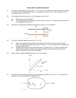


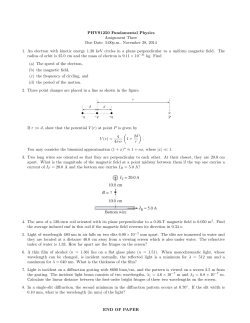
© Copyright 2026