1. science
2. physics

Gluon Transport Equation with Effective Mass and
Dynamical Onset of Bose-Einstein Condensation
Jean-Paul Blaizota , Yin Jiangb , Jinfeng Liaob,c
arXiv:1503.07260v1 [hep-ph] 25 Mar 2015
a Institut
de Physique Th´
eorique (IPhT), CNRS/URA2306, CEA Saclay,
F-91191 Gif-sur-Yvette, France
b Physics Department and Center for Exploration of Energy and Matter, Indiana University,
2401 N Milo B. Sampson Lane, Bloomington, IN 47408, USA
c RIKEN BNL Research Center, Bldg. 510A, Brookhaven National Laboratory, Upton, NY
11973, USA
Abstract
We study the transport equation describing a dense system of gluons, in the
small scattering angle approximation, taking into account medium-generated
effective masses of the gluons. We focus on the case of overpopulated systems
that are driven to Bose-Einstein condensation on their way to thermalization.
The presence of a mass modifies the dispersion relation of the gluon, as compared
to the massless case, but it is shown that this does not change qualitatively the
scaling behavior in the vicinity of the onset.
1. Introduction
In previous papers [1, 2] it was argued that a dense system of gluons such
as those created in the early stages of an ultra-relativistic heavy ion collision,
could be driven to Bose-Einstein condensation, as the system evolves towards
thermal equilibrium. This was inferred from a detailed study of the kinetic
equation that takes into account 2 to 2 scattering, in the small scattering angle
approximation. Overpopulation means that the dimensionless number n/3/4 ,
where n is the number density and the energy density, exceeds its value in
equilibrium. An overpopulated system has too many gluons, relative to its
total energy, to be accommodated in a Bose-Einstein distribution, and thermal
equilibrium requires the formation of a condensate.
Of course, such a condensate will develop provided the approach to thermal
equilibrium proceeds with conservation of both energy and particle number.
While energy is certainly conserved, inelastic processes of various kinds may
change the number of gluons (see e.g. [3, 4])1 , eventually preventing the formation of a condensate in the true equilibrium state. However, particle number
may be approximately conserved during much of the evolution, and this could
1 Note that quark production, although it decreases the number of gluons, does not necessarily hinds the formation of a condensate[4].
Preprint submitted to Elsevier
March 26, 2015
be enough to approach condensation. Indeed, transport calculations indicate
that the amplification of soft modes is a very rapid process, that a chemical
potential is indeed dynamically generated and that the onset for condensation
can be reached on short time scales. This is confirmed by calculations using the
small angle approximation [2], as well as complete solution of the Boltzmann
equation [5, 7]. There are also indications that inelastic processes could accelerate the amplification of soft modes [6], while the authors of Refs. [8] and [9]
seemingly reach a different conclusion.
Clearly the analysis of inelastic scatterings requires further work, but this is
beyond the scope of this paper. Motivation for studying the possibility for gluons
to condense comes of course from the desire to better understand how matter
produced in a high energy nucleus-nucleus collision evolves towards local thermal
equilibrium (see [10, 11] for a recent review). But, as we already emphasized in
[2], the general issue of the dynamical formation of a condensate is an interesting
problem in itself. It is of relevance in the context of cosmology (see e.g. [12]),
or cold atom physics (see e.g. [13]). It has be studied using kinetic theory,
or classical field simulations (see e.g. [14, 15]). In the context of Quantum
Chromodynamics, the nature of the condensate remains an interesting, but
unsolved, question (for a recent study in a related context, see [16]).
Our goal in this paper is to pursue our general study of the phenomenon
within kinetic theory, using a transport equation that incorporates properly
the effects of Bose statistics. The fact that the interactions are long range
interactions validate the use of the small angle approximation which reduces
the transport equation to a Fokker-Planck equation, much easier to solve than
the Boltzmann equation, thereby providing more direct analytical insight. This
paper, as well as a companion paper, addresses issues that were not discussed
in Ref. [2] which is limited to the study of the onset of condensation. We want
to extend our work so as to be able to obtain a complete dynamical description
of the approach to equilibrium including the formation of a condensate. In
order to do so, we need to attribute finite masses to the gluons. Such masses
are automatically generated by the coupling to thermal fluctuations, and the
proper transport equations that incorporate such self-energy corrections could
be derived from first principles. However, for the purpose of the present study,
it is sufficient to just give the gluons a mass, and correct appropriately the
scattering matrix element. In fact two masses will be introduced. The screening
mass mD regulates the infrared behavior of the collision kernel. The other mass,
m, modifies the dispersion relation, and one of the issues that we want to study
is how this modification changes the onset of Bose-Einstein condensation. We
shall see that, in fact, qualitatively it does not. Finally, the role of the mass m
is to allow a clear definition of the equations that describe the evolution of the
system beyond the onset, that is, in the presence of the condensate. This will
be discussed in a companion paper [17].
The outline of this paper is as follows. In the next section, we re-derive
the approximate form of the transport equation in the small scattering angle
approximation, paying attention to the presence of finite masses, and emphasizing the differences with the massless case discussed in [2]. In section 3, we
2
present results of numerical solutions of the transport equation, illustrating the
role of the mass on generic features of thermalization in both the underpopulated and overpopulated situations. In section 4, we focus on the critical regime
that accompanies the onset of condensation. We show in particular that the
change of the dispersion relation, from ultra-relativistic in the massless case,
to non-relativistic in the massive case, does not change qualitatively the scaling
regime. Details on the analytic calculation, as well as on the numerical solution,
are given in two appendices.
2. Derivation of the Transport Equation in the Massive Case
In this Section, we derive the transport equation, under the approximation
of small scattering angle, taking into account medium-induced effective masses
for both the colliding gluons and the exchange gluons.
2.1. Generalities
As in our previous papers [1, 2], we assume a transport equation for the
single particle distribution of the following form
Dt f1
= C[f ]
Z
d3 p2
d3 p3
d3 p4
1
1
| M12→34 |2
=
3
3
3
2
(2π) 2E2 (2π) 2E3 (2π) 2E4 2E1
× (2π)4 δ(P1 + P2 − P3 − P4 )
×
{f3 f4 (1 + f1 )(1 + f2 ) − f1 f2 (1 + f3 )(1 + f4 )}
(1)
where
Dt ≡ ∂t + v 1 · ∇,
(2)
and the factor 1/2 in front of the integral is a symmetry factor. Summation over
color and polarization is performed on the gluons 2,3,4; average over color and
polarization is performed for gluon 1. The distribution function f is a scalar
object (i.e., independent of color and spin):
f (x, p) =
dN
(2π)3
,
2
3
2(Nc − 1) d xd3 p
(3)
where N denotes the total number of gluons. In other words, f denotes the number of gluons of a given spin and color in the phase-space element d3 xd3 p/(2π)3 .
We consider a uniform system, so that f is in fact independent of x. Also, in
this paper, we consider a non-expanding system, so that Dt = ∂t . Finally, Pi
denotes the four-momentum of particle i, Pi = (Epi , pi ).
In this paper, contrary to our previous work, we assume that the gluons
carry a small mass, arising from their interactions with the medium. This is
a crude approximation to the true self-energy, but our main goal here is not
to give a quantitative description of the phenomenon, but rather to study how
the onset of Bose-Einstein condensation is affected by such a mass. We believe
3
that a more complete, but much more difficult, treatment would not change our
main conclusions. The major change brought by the presence of the mass is
that of the dispersion relation
of the modes. Thus the energy of a particle with
p
momentum p is Ep = p2 + m2 .
It is convenient to express the final momenta in terms of the initial ones and
of the momentum q transferred in the collision. We set
p3 = p1 + q,
p4 = p2 − q.
(4)
One can then perform the integrations over p3 and p4 using the three-momentum
delta function. We get
Z Z
C[f ] =
w(p1 , p2 , q){f12→34 },
(5)
p2
q
with
w(p1 , p2 , q) ≡
πδ(E1 + E2 − E3 − E4 )
| M12→34 |2 ,
16E1 E2 E3 E4
(6)
and
{f12→34 } ≡ f3 f4 (1 + f1 )(1 + f2 ) − f1 f2 (1 + f3 )(1 + f4 ),
(7)
where fi is a shorthand notation for fpi . The quantity w(p1 , p2 , q) may be interpreted as the rate of collisions of particle 1 with particle 2, in which momentum
q is transferred to particle 1, its momentum p1 becoming p1 + q. Note that the
symmetry factor is included in the definition of w. The (dimensionless) matrix
element M12→34 will be discussed shortly. It is understood in the expressions
above that the momenta p3 and p4 are expressed in terms of p1 , p2 , q according
to (4). Also, we used the shorthand for momentum integration
Z
Z
d3 p
.
(8)
≡
(2π)3
p
Note that the symmetries of the matrix element (see below) entail the property
w(p1 , p2 , −q) = w(p1 , p2 , q) = w(p2 , p1 , −q).
(9)
2.2. The small scattering angle approximation and the Fokker-Planck equation
Under the small scattering angle approximation, the momenta of incident
particles get changed very little during each collision, and the kinetic equation
can be approximated by a Fokker-Planck equation in momentum space [18].
Following a standard procedure [19], we write the collision integral as
C[f ] = −∇ · J = −
∂Ji
.
∂pi
(10)
Note the gradient ∇ in the above, and for the rest of this paper, is the momentum space gradient i.e. ∇ = ∇p . In order to estimate Ji , the component of the
4
current (of particles 1) in the direction i (with i = 1, 2, 3), we count the number
of particles that, as a result of collisions during the interval dt, cross a surface
¯ of p1 .
element orthogonal to the direction i and located at a particular value p
An elementary analysis yields
Z
Z Z p¯i
Ji =
dpi w(p1 , p2 , q)
q, qi >0
×
p2
p¯i −qi
fp1 fp2 (1 + fp1 +q ) (1 + fp2 −q ) − (1 + fp1 ) (1 + fp2 ) fp1 +q fp2 −q ,
(11)
where the q-integration is restricted to positive components qi . In the small
angle approximation the combination of statistical factors simplifies into
fp1 fp2 (1 + fp1 +q ) (1 + fp2 −q ) − (1 + fp1 ) (1 + fp2 ) fp1 +q fp2 −q
≈ q · hp1 (∇f )p2 − hp2 (∇f )p1 + O(q 2 ),
(12)
where we have introduced the notation hp ≡ fp (1 + fp ). In addition, we notice
that, in this approximation, the energy conservation implies
0 = q · v 1 − q · v 2 + O(q 2 ).
(13)
By taking all these together we obtain the following leading order expression
for the momentum flux:
Z Z
1
q i w(p1 , p2 , q) q · hp1 (∇f )p2 − hp2 (∇f )p1 .
(14)
Ji =
2 q p2
Note that in the above equation we have relaxed the constraint qi > 0 on the
q-integration, dividing the result by 2 (using the fact that the integrand is even
in q, see Eqs. (9)). We can rewrite the current as follows
Z
Ji =
B ij (p1 , p2 ) hp1 (∇j f )p2 − hp2 (∇j f )p1 ,
(15)
p2
with the (dimensionless) angular tensor
Z
1
B ij (p1 , p2 ) =
q i q j w(p1 , p2 , q).
2 q
(16)
2.3. Conservation laws
The particle number conservation is obvious due to the structure of the
collision term as the divergence of a current:
Z
C[fp1 ] = 0
(17)
p1
5
To prove the energy conservation requires a little more effort
Z
Z
Ep1 C[fp1 ] = −
Ep1 ∇p1 · J (p1 )
p1
p
Z 1
Z
= −
∇p1 · Ep1 J (p1 ) +
∇p1 Ep1 · J (p1 )
Z
=
=
=
=
p1
3
p1
d p1
v 1 · J (p1 )
(2π)3
Z Z Z
1
w(p1 , p2 ; q)
2 p1 p2 q
×(v 1 · q) q · hp1 (∇f )p2 − hp2 (∇f )p1
Z Z Z
1
w(p1 , p2 ; q)
2 p1 p2 q
× (v 1 · q) hp1 (q · ∇f )p2 − (v 2 · q) hp2 (q · ∇f )p1 ,
0
(18)
where in the last steps we have used Eq.(13) and Eqs. (9).
2.4. The matrix element
The matrix element for (in vacuum) gluon-gluon scattering (1 + 2 → 3 + 4)
reads (spin and color averaged for 1, and summed for 2,3,4)
tu su ts
2
2 2 2
128π 2 αs2 Nc2 = 72g 4 ,
(19)
| M | = 128π αs Nc 3 − 2 − 2 − 2 ,
s
t
u
with s, t, u the standard Mandelstam variables:
s = (P1 + P2 )2 ,
t = (P1 − P3 )2 ,
u = (P1 − P4 )2 .
(20)
In the small scattering angle approximation, the dominant contributions
come from the kinematic regions t ≈ 0 and u ≈ 0. With the vacuum matrix
element and in massless case, one would have the following approximation:
tu su ts
su ts
s2
| M |2 = 72g 4 3 − 2 − 2 − 2 ≈ 72g 4 − 2 − 2 ≈ 144g 4 2 , (21)
s
t
u
t
u
t
where in the last step we have used the fact that the two contributions are equal,
and, for massless particles, u = −(s + t) ≈ −s (for t ≈ 0).
Now we consider the modifications of the matrix elements that need to be
taken into account when the gluons are massive. There are two distinct physical
effects. One is the screening of the t-channel singularity. This should be taken
care of by separating the transverse and the longitudinal channels, and including
the proper polarization tensors in the exchange gluons. In this paper we simply
modify the denominator by substituting t → t − m2D , with mD a screening mass
whose main role here is that of a regulator. The other physical effect is coming
6
from self-energy corrections on the external lines. As already mentioned, we
simply take these into account by giving the gluon a small thermal mass m,
allowing m to differ from mD . In summary, we replace the matrix element
derived for massless particles by
| M |2 → 144g 4
s2
,
(t − m2D )2
s ≈ 2E1 E2 (1 − v 1 · v 2 ),
(22)
where v i = pi /Ei is the velocity of particle i, and since we are interested in the
small m limit, we dropped a term ∼ m2 in the expression of s. With that, we
then obtain, in the leading order of the small scattering angle approximation
w = 36πg 4 δ(q · v 1 − q · v 2 )
(1 − v 1 · v 2 )2
(ω 2 − q 2 − m2D )2
where ω = v 1 · q.
With this matrix element, the angular tensor takes the form
Z
(1 − v 1 · v 2 )2
B ij (p1 , p2 ) = 18πg 4
δ(v 1 · q − v 2 · q)q i q j 2
.
(ω − q 2 − m2D )2
q
(23)
(24)
2.5. The isotropic case
We assume that
p the distribution function is a function of the energy, fp =
f (Ep ) with Ep = p2 + m2 . In such case we have the following relation
∇fp = v f 0 (Ep ),
f 0 (E) ≡
df (E)
,
dE
(25)
with the velocity given by v = p/Ep = ∇p Ep . Then we have
hp1 (∇j f )p2 − hp2 (∇j f )p1 = v j2 h1 f20 − v j1 h2 f10 ,
(26)
where we introduced the simplified notation fi = f (Ei ) = fpi (and similarly for
hi ) that will be used throughout the paper.
In this isotropic case, the calculation of the angular tensor (24) simplifies.
In particular, the current J~ (p) is a vector aligned with the direction of p, that
ˆ 1 = p1 /p1 )
is (with p1 = |p1 | and p
ˆ 1 J (p1 ).
J~ (p1 ) = p
(27)
It follows that the kinetic equation can be written as
Dt f1 = −
1
∂p1 p21 J (p1 ) .
2
p1
The calculation presented in Appendix A yields
Z
J (p1 ) = 36παs2
(h1 f20 − h2 f10 )Z(v1 , v2 ),
(28)
(29)
p2
where the explicit expressions of the dimensionless function Z(v1 , v2 ) is given
in Appendix A.
7
2.6. The massless limit
It is shown in Appendix A.4 that the current at small momentum has the
following structure
p1
− J (p1 → 0) ' 36παs2 L Ia (p1 )∂p1 f1 +
Ib (p1 )h1 ,
(30)
E1
where L is a positive constant, and (see Eq. (A.25))
Z
Z
Z
p1
h2
p1
f20
p1
1
∂ p f2 .
Ia (p1 ) ≡
, Ib (p1 ) ≡ −
=−
m p 2 v2
m p 2 v2
m p2 v22 2
(31)
This structure is identical to that obtained in the massless limit [2], with the
integrals Ia and Ib given by
Z
Z
2f (p)
Ia =
f (p)(1 + f (p),
Ib =
.
(32)
p
p
p
We shall end this section by making a general comment on the Fokker-Planck
equation in this massless limit, in order to clarify the interpretation of the two
competing terms that are present in the current. For simplicity we focus on the
isotropic case so that the kinetic equation is of the form2
1
∂p p2 [Ia ∂p f (p) + Ib f (1 + f )] .
2
p
R
Note that energy conservation, ∂t p pf (p) = 0, entails
Z
Z
∂f
Ia
= Ib f (1 + f ),
p ∂p
p
∂t f (p) =
(33)
(34)
a relation that is obviously satisfied given the definitions (32) of Ia and Ib .
To gain insight into the physical meaning of the two terms on the r.h.s. of
this equation, let us multiply both sides by p2 and integrate over momentum.
We obtain
Z
Z
1
(35)
∂t p2 f (p) =
p2 2 ∂p p2 [Ia ∂p f (p) + Ib f (1 + f )] .
p
p
p
Using integration by part for the r.h.s., we eventually obtain
˜
∂t hp2 i = 6Ia hni − 2Ib hpi,
(36)
where
hp2 i ≡
Z
p
p2 f (p),
Z
hni ≡
f (p),
p
˜ ≡
hpi
Z
pf (1 + f ).
(37)
p
2 We absorb here the constant factor 36πα2 L into the redefinition of time (see Eq. (38)
s
below).
8
The equation (36) may be interpreted as follows. The first term on the r.h.s.,
6Ia hni, represents the diffusion of particles in momentum space that results
from multiple small-angle scatterings. If this first term was the only one, the
system would diffuse indefinitely, with hp2 i ∼ Ia hnit at late time. The second
˜ represents a drag force, with the characteristic of
term on the r.h.s., −2Ib hpi,
a friction. It is negative as long as there is any nonzero momentum in the
system and therefore opposes the diffusive contribution, which is generically
positive. In the absence of diffusion, this term would cause the magnitude of
the momentum to decrease continuously, eventually bringing all particles to a
state of zero momentum. This drag term is the agent that drives the system
towards condensation. Finally, with both terms present on the r.h.s of the
equation, thermal equilibrium can be reached, and the system approaches the
fixed point corresponding to a Bose-Einstein distribution, with T = Ia /Ib .
3. Numerical solutions to the transport equation
We turn now to the discussion of results obtained by solving numerically the
Fokker-Plank equation for relevant cases. Details on the numerical procedure
that we used can be found in Appendix B. We shall write the transport equation
in terms of dimensionless quantities. In order to do so, we express all momenta
(and masses, energies, temperature) in units of Qs , and the time in units of
1/Qs . In fact, we also absorb into the dimensionless time a numerical factor,
setting
τπ
1
.
(38)
t≡
Qs 18αs2
This is the factor that should be used if one wants to relate the time τ of the
simulation to the physical time t. 3
In the dimensionless variables, the transport equation reads
Z
1
Dτ f (p) = − 2 ∂p p2 J (p) ,
J (p1 ) =
(h1 f20 − h2 f10 )Z(v1 , v2 ).
p
p2
(39)
Note that since from now on we shall be dealing mostly with dimensionless variables, we keep the same names for the dimensionful and dimensionless momenta.
The initial condition is chosen
p be of the Glasma type [1], i.e. f (E) =
p2 + m2 . For this family of initial condif0 (1 + e10(E−1.5) )−1 , with E =
tions, there is a critical value of f0 , that we call f0c , above which the system
becomes overpopulated. When f0 = f0c , the equilibrium distribution is a BoseEinstein distribution with a maximal chemical potential µ = m. The value of
3 Note that this factor differs by a factor 2π 2 L from the “natural” factor that appears for
instance in the expression (29) of the current. Note that π/(18α2s ) ≈ 0.7 so that t ≈ τ /Qs .
9
1.4
3
10
1.2
2
10
(p=0)
0
c
1.0
0.8
1
10
0.6
0
10
0.4
-1
10
0.2
0.2
0.4
m
0.6
0.8
0.0
1.0
0.2
0.4
0.6
/
0.8
1.0
c
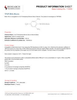
Figure 1: (Color online.) Left: Critical f0 as a function of the gluon mass m. Points above
the curve correspond to overpopulated initial conditions, below the curve to underpopulated
initial conditions. Right: The evolution of f (p ≈ 0) for different initial occupations f0 (with
m = 0.3): the lower (black) curve is for underpopulated initial condition, and the other curves
are for overpopulated initial conditions.
f0c depends on the mass m of the gluons, and its variation with m is illustrated
in Fig. 1. It is seen that f0c increases with m: the value of f0 required to reach
the onset of condensation is larger for massive particles than for massless ones.
The right hand panel of Fig. 1 illustrates the behavior of f (p = 0) in the two
generic situations of underpopulation where f (0) reaches a constant value and
that of overpopulation where f (0) diverges at a finite time τ = τc .
Note that in all cases, the infrared part of the distribution function evolves
rapidly towards an approximate classical thermal distribution function,
f (E) →
T∗
(E − µ∗ )
(40)
with an effective temperature T ∗ and effective chemical potential µ∗ that can
be determined numerically. The evolution of T ∗ and µ∗ with time depends
on whether the system is over or underpopulated, as we shall discuss in the
following.
3.1. Underpopulated case
Starting from the initial distribution corresponding to underpopulation, we
verify that the system evolves to the expected equilibrium state. The approach
to thermalization is illustrated in Fig.2 which displays the evolution of the distribution function f (p) and that of the current J (p). The current changes its
sign around E ' 1.3, the point which separates the effects of the two competing components of the current. For larger values of E, the current is diffusive
and positive. For smaller values of E, the current is dominated by its drag
component, and is negative. As time progresses these two components of the
current move particles in momentum space, the drag term pushing particles towards small momenta, the diffusion term smoothening the distribution at large
10
2
0.8
1
0.6
0
-1
0.4
-2
0.2
-3
-4
0.0
0.4
0.8
E
1.2
1.6
0.4
2.0
0.8
1.2
1.6
E
2.0
Figure 2: Left: Distribution function f (E) at various times τ =0.05, 0.8, 1.4, 6.25 (from
bottom to top at E = 0.4). Right: Current J at τ =0.05, 0.8, 1.4, 6.25 (from bottom to top
at E = 0.4). Underpopulated initial condition, with m = 0.3 and f0 = 0.1.
momenta. The resulting distribution gradually evolves towards the equilibrium
distribution, as indicated in the left panel of Fig. 2, while the current diminishes,
and eventually vanishes (which takes place approximately for the largest time
considered in the plot). The evolution with time of the effective parameters that
characterize the infrared part of the distribution function are displayed in Fig. 3.
This figure clearly demonstrates that the system thermalizes as expected.
0
2.0
-1
1.6
T
*
-2
1.2
-3
0.8
-4
0.4
-5
0
1
2
3
4
5
0
6
1
2
3
4
5
6
Figure 3: (Color online.) The evolution with time of the effective local temperature T ∗
(left) and chemical potential µ∗ (right) for an underpopulated initial condition (m = 0.3 and
f0 = 0.1). At late time, both quantities approach their expected equilibrium values, indicated
by the horizontal (red) dotted lines.
3.2. Overpopulated cases
We turn now to the situation with overpopulation. We expect, from our
previous work, that the system will approach the onset of condensation in a
finite time τ = τc . We have studied the evolution with different masses(m =
0.1, 0.3, 0.5, 0.7). In the numerical solution, the time step is self-adaptive i.e.
11
becoming smaller when the evolution becomes faster, which allows us to evolve
the system in each case very close to the onset. The evolution is stopped when
f > 800 for the smallest momentum grid point, which roughly corresponds to
the situation when the difference between the local chemical potential µ∗ and
the mass becomes less than the mesh size. That is, the evolution is stopped
very near the onset of condensation where µ = m. An illustration of the energy
dependence of the distribution near the onset is displayed in Fig. 4
0.025
0.015
f
-1
0.020
0.010
0.005
0.000
0.300
0.305
E
0.310
0.315
Figure 4: The inverse of the distribution as a function of energy, 1/f versus E, for m = 0.3,
and τ = 0.101 corresponding to the onset of condensation.
The Table 1 gives some typical values of the parameters f0c and τc for different initial conditions, and different values of the mass m and the Debye mass
mD . One notices that, for fixed masses (e.g. m=0.3) the onset time decreases
with increasing f0 , which is as expected: the larger the overpopulation, the
shorter time it takes to reach the onset of BEC. For fixed m and f0 an increase
of the Debye mass leads to an increase of τc (compare for instance the lines
corresponding to m = 0.7 and f0 = 1). This is because an increase of mD
reduces the scattering rate, which slows down the evolution. A larger increase
of τc results from the increase of m at fixed f0 and mD . The latter phenomenon
is in line with what we observed earlier, namely that f0c increases with m.
Different from the underpopulated case, the evolution of the flow of particles
is quite different in the overpopulated case, as shown in Fig.5 . The negative
infrared flux keeps increasing in a roughly self-similar manner. The local chemical potential µ∗ approaches µc = m at the onset. We have extracted the µ∗
as a function of time for a variety of mass values as well as initial occupation
values: see Fig.6. In all cases, we have found that the evolution of µ∗ close to
the onset point can be fitted with power law µ = m − λ (τc − τ )η . Furthermore
in all cases, we’ve found the optimal exponent is about one, i.e. η ' 1. This
dynamical behavior in the present massive case is essentially the same as that
12
m
mD
f0
f0c
τc
0.1
0.3
0.5
0.7
0.3
0.3
0.3
0.3
0.3
0.1
0.7
0.1
0.3
0.5
0.7
0.3
0.3
0.3
0.3
0.3
0.7
0.1
1.0
1.0
1.0
1.0
1.2
1.4
1.6
1.8
2.0
1.0
1.0
0.271
0.508
0.747
0.969
0.508
0.508
0.508
0.508
0.508
0.271
0.969
0.029
0.101
0.259
0.663
0.065
0.046
0.034
0.026
0.021
0.095
0.242
Table 1: Critical occupation factor f0c and onset time scale τc for different combinations of
parameters.
3
10
0
4
-1x10
4
2
-2x10
10
4
-3x10
4
-4x10
1
4
10
-5x10
4
-6x10
4
-7x10
0
10
-4
10
-3
10
-2
10
-1
10
0
-4
10
10
E-m
-3
10
-2
10
-1
10
E-m
Figure 5: Color online. Distribution function f (left) and current [J ] (right), the curves
corresponding, from bottom to top, to increasing values of τ : τ =0.04(black), 0.0674(red),
0.0871(green), 0.0927(blue), 0.0961(yellow), 0.0977(pink) with m = 0.3 and f0 = 1.0 (overpopulated initial condition).
found for the massless case in [2]. We give a more complete discussion of this
regime in the next section.
4. Critical scaling analysis
In this section we examine how the scaling behavior that holds near the
onset of BEC is affected by the gluon mass. A major modification, with respect
to the massless case, concerns the dispersion relation near the onset. When
m 6= 0, condensation occurs
p when m = µ, and the dispersion relation becomes
non relativistic, Ep −µ = p2 + m2 −m ≈ p2 /(2m), which differs from the ultra
relativistic dispersion relation of the massless case, Ep = p, where condensation
13
0
10
1.00
1.00
0.98
/ m
*
/ m
0.98
0.96
*
0.94
0.96
0.94
0.92
0.92
0.90
0.65
0.70
0.75
0.80
0.85
0.90
0.95
0.90
1.00
0.2
0.4
c
0.6
0.8
1.0
c
Figure 6: Evolution of IR local chemical potential µ∗ toward onset µ∗ → m for different
choices of f0 =1.0, 1.2, 1.4, 1.6, 1.8(from left to right) with the same mass m = 0.3. Right:
Evolution of IR local chemical potential µ∗ toward onset µ∗ → m for different choices of
external mass m =0.7, 0.5, 0.3, 0.1(from left to right) with the same f0 = 1.
occurs at µ = 0. This change in the dispersion relation modifies the singularity
near the onset, but, as we shall see, this does not affect in a major way the
onset critical behavior. The foregoing analysis follows closely that presented in
Ref. [2].
4.1. Scaling behavior of the current at small momentum
As we have seen in solving numerically the Fokker-Planck equation, for
generic initial conditions, the distribution function at small momentum evolves
rapidly towards the approximate equilibrium distribution:
T∗
2mT ∗
2mT ∗
≈
=
,
(41)
E(p) − µ∗
p2 + 2mδµ
p2 + ∆ 2
√
where we have set δµ ≡ m − µ∗ and ∆ ≡ 2mδµ. As the system approaches
condensation, ∆ → 0. To analyze the detailed behavior of the properties of the
system when ∆ → 0, it is convenient to calculate the time dependence of the
number of particles inside a small sphere of radius p0 centered at the origin.
In doing this calculation, we assume that f (p) keeps the form (41), with time
dependent parameters T ∗ and δµ. In particular, f (0) remains finite as long as
δµ 6= 0. A simple calculation then yields
Z p0
∂τ
dpp2 f (p) = 2m∆(∂τ T ∗ )h1 (y) + 2mT ∗ (∂τ ∆)h2 (y),
(42)
f (p) ≈
0
where y ≡ p0 /∆, and the two scaling functions are
= y − ArcTan(y)
y
h2 (y) =
− ArcTan(y).
1 + y2
h1 (y)
14
(43)
(44)
By using Eq. (28), one can relate the left hand side of Eq. (42) to the current
at p0 , and obtain
Rp
∂τ 0 0 dpp2 f (p)
2m(∂τ T ∗ ) h1 (y) 2mT ∗ (∂τ ∆) h2 (y)
− J (p0 ) =
=
+
. (45)
2
p0
∆
y2
∆2
y2
This equation provides interesting constraints on the small p behavior of J (p).
In the limit y → 0 or p0 ∆, one gets
∗
∗
1
2m
T
T
p0
=
p
×
− J (p0 ) ' p0 ×
∂τ
∂
= ∂τ f (0).
(46)
0
τ
3
∆2
3
δµ
3
The current is linear in p0 , with a slope proportional to ∂τ f (0), very much like
in the massless case [2]. On the other hand, in the limit y 1 or ∆ p0 T ∗ ,
one obtains the following leading order result4
− J (p0 ) →
1
× (πm)∂τ (−T ∗ ∆).
p20
(47)
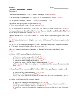
In this region, the current exhibits a singular behavior in 1/p20 . The value
(≈ ∆) of the momentum where the change of regime occurs decreases with
time, while the absolute value of the current at the minimum becomes larger
and larger, and eventually diverges at the onset. This behavior is illustrated in
Fig. 7. As was the case in the massless case, the current in the scaling regime is
dominated by the second term in Eq. (45). One also finds that the dependence
of m − µ∗ on τc − τ is linear. A discussion of the latter point is presented in
Appendix Appendix A.4.
5. Summary
In this paper, we have extended the analysis carried out in Ref. [2] to the case
where the gluons are given a small mass m. The main difference with respect
to the massless case studied in [2] is the change of the dispersion relation of the
gluon modes, from ultra-relativistic in the massless case to non-relativistic in the
massive case. While this change in the dispersion relation leads to an enhanced
singularity of the distribution function near the onset of Bose condensation, from
1/p to 1/p2 , we find that the critical regime that accompanies the approach to
the onset is qualitatively unchanged. The Debye mass mD controls the infrared
behavior of the collision kernel. It is kept constant, and independent of m,
although in a more complete theory, both masses are related, and would depend
on the temperature. However this is expected to have little impact at the onset,
since the onset process is dominated by a critical regime where the actual value
of the mass is irrelevant. We have checked in articular that letting the Debye
4 The subleading contribution is ∼ 1/p and comes from the first term in Eq. (45). It
becomes the dominant contribution after onset, when δµ = 0 and therefore (47) vanishes.
15
0.0
0
4
-1x10
-0.5
4
-2x10
4
J
-3x10
-1.0
4
-4x10
4
-5x10
4
-6x10
-1.5
4
-7x10
0.0
0.2
0.4
p
0.6
0.8
0.0
0.1
0.2
p
0.3
0.4
Figure 7: The current (in arbitrary units) as a function of momentum, at different time
moments (earlier to later time from top to bottom) close to onset. Left panel: calculated
according to the formula (45), assuming a linear relation between µ∗ − m and τc − τ , and
neglecting the time variation of T ∗ ; right panel: obtained from the numerical solution. The
linear behavior at small p followed, as p increases, by a singular behavior in 1/pα , with α > 0
is clearly visible on both figures.
mass adjust with temperature as one approaches BEC does not lead to any
significant changes in the behavior of the system. Finally, the presence of the
mass m allows us to define properly the equations that governs the dynamics
beyond the onset, that is, in the presence of the condensate. This is discussed
in a companion paper [17].
Acknowledgements
The research of JPB is supported by the European Research Council under
the Advanced Investigator Grant ERC-AD-267258. That of YJ and JL is supported by the National Science Foundation under Grant No. PHY-1352368. JL
is also grateful to the RIKEN BNL Research Center for partial support.
Appendix A. Derivation of the current J (p)
The component i of the current J (p1 ) in Eq. (15) can be written
Z
Z 3
d3 q
d p2
i
4
0
0
J (p1 ) = 18πg
3
3 (h1 f2 − h2 f1 )
(2π)
(2π)
×
q i (q · v 2 )
(1 − v 1 · v 2 )
2
2
2
[(v 1 · q) − q 2 − m2D ]
16
δ(q · v 1 − q · v 2 ).
(A.1)
0.5
Appendix A.1. Details of the angular integration
In order to perform the angular integrals, we choose the following coordinate
frames: We define the orientation of q in a frame where p1 is along the zˆ axis,
and denote the corresponding angles by θ and φ. The orientation of p2 , given
p1 and q, is defined by the angles θ2 , φ2 in a frame with q along zˆ2 and q, p1
spanning the x
ˆ2 -ˆ
z2 plane. We have therefore q ·v 1 = qv1 cos θ, q ·v 2 = qv2 cos θ2 ,
and v 1 · v 2 = v1 v2 (cos θ cos θ2 + sin θ sin θ2 cos φ2 ).
By integrating over φ2 one gets
R 2π
R 2π
dφ2 (1 − v 1 · v 2 )2 = 0 dφ2 [1 − v1 v2 (cos θ cos θ2 + sin θ sin θ2 cos φ2 )]2
0
= π[2(1 − v1 v2 cos θ cos θ2 )2 + v12 v22 (1 − cos2 θ)(1 − cos2 θ2 )]
(A.2)
Furthermore we rewrite the delta function as
qδ(q · v 1 − q · v 2 ) = qδ(q(v1 cos θ − v2 cos θ2 )) = δ(v1 cos θ − v2 cos θ2 ) (A.3)
= θ(v1 − v2 )δ(v1 cos θ − v2 cos θ2 ) + θ(v2 − v1 )δ(v2 cos θ2 − v1 cos θ)
and change variables, setting x1 = v1 cos θ, x2 = v2 cos θ2 . One can then complete the angular integration. Note that, by symmetry, the current is aligned on
ˆ 1 J (p1 ), with J (p1 ) a function of p1 = |p1 |
the direction of p1 , i.e., J~ (p1 ) = p
ˆ 1 = p1 /p1 .. We get
only, and p
Z
Z
18αs2
dq Z(v1 , v2 , cq )
2
0
0
J (p1 ) =
dp2 p2 (h1 f 2 − h2 f1 )
,
(A.4)
π
q
v1
with
v1 v2 Z(v1 , v2 , cq )
=
1
2
Z
"Z
2
v2
dx2 x22
2(1 − x22 ) + (v12 − x22 )(v22 − x22 )
2
(x22 − cq )
−v2
dx1 x21
2(1 − x21 ) + (v12 − x21 )(v22 − x21 )
2
(x21 − cq )
−v1
=
+
+
+
#
2
v1
+
θ(v1 − v2 )
θ(v2 − v1 )
h
v v 2 − 6(1 − cq ) + (1 − v12 ) + (1 − v22 )
#
2
(1 − cq )
(cq − v12 )(cq − v22 )
+
cq − v 2
2(cq − v 2 )
"
2
(1 − cq )
(cq − v12 )(cq − v22 )
−
−
− (1 − v12 ) − (1 − v22 )
cq
2cq
i√
v
6(1 − cq ) cq ArcTanh √
,
(A.5)
cq
where cq = 1 + m2D /q 2 , v = min(v1 , v2 ), and we have used the following integral
17
formula to get the final results
"
#
Z
A
B
2
dx x 3C +
+
(A.6)
2
c0 − x 2
(c0 − x2 )
√
A
x
Ax
+
B
c
−
ArcTanh
,
= Cx3 − Bx −
√
√
0
2(x2 − c0 )
2 c0
c0
with A = 2(c0 − 1)2 + (c0 − v12 )(c0 − v22 ), B = 4 + v12 + v22 − 6c0 , C = 1.
Appendix A.2. Limiting cases
There are a few limiting cases where the expression above simplifies. For
instance, in the limit of vanishing screening mass mD → 0, cq = 1 and
(1 − v12 )(1 − v22 )
2
2
2
v1 v2 Z = v v + (1 − v1 ) + (1 − v2 ) −
2(1 − v 2 )
2
2
(1 − v1 )(1 − v2 )
2
2
+
− (1 − v1 ) − (1 − v2 ) ArcTanh(v). (A.7)
2
In this limit, the remaining q-integration in theRexpression (A.4) of the current
becomes simply the usual Coulomb logarithm, dq/q → L.
In the limit where all effective masses vanish, i.e. m → 0 and mD → 0, cq
and all the velocities become unity, v1 v2 Z → 1 and we recover the expression
of the massless case studied in Ref. [2].
In the limit where the colliding gluons become massless, i.e., m → 0, but the
Debye mass stays finite, all the velocities v1 , v2 , v approach unity, and we get
15
v1 v2 Z =
1 − (1 − cq )
2
3(1 − cq )
1
√
+ cq (1 − cq ) −
+ 6 ArcTanh √
. (A.8)
2cq
cq
This expression is finite when q → 0. To see that, recall that when q → 0,
cq ∼ m2D /q 2 → ∞. As simple calculation then yields
−3
v1 v2 Z ≈ A c−2
q + O(cq ),
(A.9)
where
A=
3 7 v5
v3
v − (4 + v12 + v22 ) + (2 + v12 v22 )].
7
5
3
(A.10)
This result confirms that in the presence of a non-vanishing screening mass mD ,
the function Z is regular as q → 0, and the q-integration in the expression (A.4)
becomes infrared finite, as expected.
18
Appendix A.3. Detailed derivation of the q-integration
In the general case, in order to perform the q-integration in Eq. (A.4), we
rewrite v1 v2 Z in Eq. (A.5) as follows:
E1
v
√
2
v1 v2 Z(cq , v1 , v2 ) =
+ E2 (cq − v ) + E3 + cq ArcTanh √
cq − v 2
cq
cq − 1
×[E4 (1 − cq ) + E5
+ E6 ],
(A.11)
cq
where
E1
=
E3
=
E5
=
15v
v 2 2
[2v (3v − v12 − v22 − 4) + 2v12 v22 + 4],
E2 =
4
2
15
v
(20v 2 − 3v12 − 3v22 − 12),
E4 =
2
2
1
1
[−2v12 v22 − 4],
E6 = [−2v12 v22 + 6v12 + 6v22 − 10]. (A.12)
4
4
Then, we change integration variable from q to cq and obtain
Z
Z
dq
dcq
v1 v2 Z(q, v1 , v2 ) =
v1 v2 Z(cq , v1 , v2 )
q
2(1 − cq )
= E1 G1 (v, cq ) + E1 G1 (v, cq ) + E2 G2 (v, cq ) + E3 G3 (v, cq )
+E4 G4 (v, cq ) + E5 G5 (v, cq ) + E6 G6 (v, cq ).
(A.13)
The results of these integrals are listed below:
Z
ln(cq − v 2 ) − ln(cq − 1)
1
=−
G1 (v, cq ) = dcq
2
2(1 − cq )(cq − v )
2(v 2 − 1)
Z
1
cq − v 2
G2 (v, cq ) = dcq
= − [cq + (1 − v 2 ) ln(cq − 1)]
2(1 − cq )
2
Z
1
1
G3 (v, cq ) = dcq
= − ln(cq − 1)
2(1 − cq )
2
Z
v
1√
v
1
ArcTanh
G4 (v, cq ) = dcq
cq ArcTanh √
= [2c3/2
+ v 3 ln(cq − v 2 ) + cq v]
√
2
cq
6 q
cq
Z
1
v
1
v
√
G5 (v, cq ) = dcq
ArcTanh √
=
v ln(cq − v 2 ) + 2 cq ArcTanh √
2cq
cq
2
cq
(A.14)
19
1
v
ArcTanh √
2(1 − cq )
cq
√
cq
v
v
1
v2
= v{−
ArcTanh √
+ ln √
− ln 1 −
v
cq
cq
2
cq
√ √
√ 1 − v/ cq
cq − 1
v + v cq
v
1
2 ln( √
)ArcTanh √
+ Li2
+ Li2 −
−
4v
cq + 1
cq
1+v
1−v
√
√
v − v cq
1 + v/ cq
+Li2 (−
) + Li2 (
)
1−v
1+v
√
√
+ ln(v − v/ cq ) ln(1 − v/ cq ) − ln(v 2 − v 2 /cq ) ln(1 − v)
√
√ − ln(1 − v 2 /cq ) ln(1 + v) + ln(v + v/ cq ) ln(1 + v/ cq ) }.
(A.15)
Z
G6 (v, cq ) =
dcq
We define, with Λ an ultraviolet cutoff5 :
Λ
Z
0
dq
v1 v2 Z(cq , v1 , v2 ) = L(cΛ , v1 , v2 ) − L(∞, v1 , v2 ),
q
(A.16)
where the first argument of L denotes the value of cq (when q = Λ or q = 0,
respectively). As we have already shown, there is no singularity at q → 0 i.e.
cq → ∞ when mD is finite, and we have the following finite result
1
L(∞, v1 , v2 ) =
20v 3 − 12v(v12 v22 + 2)]
24
1
v
+ Li2
+ 2v − (2v + ln(1 − v)) ln(v) ,
−3 ∆ Li2
v−1
v+1
(A.17)
where ∆ = −2v12 v22 + 6(v12 + v22 ) − 10. Note in the massless limit for external
gluons, i.e. m → 0, one has ∆ → 0 and the expression above greatly simplifies:
√
√
4
1
.
(A.18)
L(cΛ ) − L(∞) = − 5cΛ + (3 − 5cΛ ) cΛ ArcCoth( cΛ ) −
2
3
We write the final result for the current in the form
Z
18αs2
J (p1 ) =
dp2 p22 Z(v1 , v2 ) [h1 f20 − h2 f10 ]
π
(A.19)
with
Z
Z(v1 , v2 )
dq Z(v1 , v2 , cq )
q
v1
2
−1
= (v1 v2 ) [L(cΛ , v1 , v2 ) − L(∞, v1 , v2 )] .
=
(A.20)
5 One expects Λ to be typically of the order of the temperature. The numerical calculations
have been performed with a somewhat larger value, Λ = 4Qs .
20
Appendix A.4. The small momentum regime
We now analyze the small momentum form of the current, J (p1 → 0). The
leading order expression of Z in the limit v1 → 0 can be obtained after a lengthy
but straightforward calculation. It reads
Z(v1 → 0, v2 ) ≈ L
v3
v12 v2
(A.21)
where v = min(v1 , v2 ), and L is a positive constant,
1
1
m2
.
L = − log(cΛ − 1) − log(cΛ ) +
,
cΛ = 1 + D
3
cΛ
Λ2
The small momentum current can therefore be written as6
Z
v3
0
0
− J (p1 ) = 36παs2 L
2 v [h2 f1 − h1 f2 ] .
v
p2 1 2
(A.22)
(A.23)
Since the numerical factor in front of the integral is to be absorbed in the
redefinition of the time scale (see Eq. (38)), we rewrite J (p1 ) as
− J (p1 ) = Ia (p1 )f10 + Ib (p1 )h1 ,
(A.24)
where
Z
Ia (p1 ) =
h2
p2
v3
,
v12 v2
Z
Ib (p1 ) = −
p2
f20
v3
v12 v2
(A.25)
These integrals reduce to the integrals Ia and Ib of Eq. (32) in the massless
limit (in this limit, the dependence on p1 disappears and L becomes the usual
Coulomb logarithm).
We argue in the main text, and we have verified through numerical calculations, that at small momentum and near the onset for BEC, the distribution function f (p) can be well approximated by a Bose equilibrium distribution
function We
√ therefore write the distribution in the momentum range of interest
(p ∆ = 2mδµ) as
f (p) = f ∗ (p) + δf (p),
(A.26)
where f ∗ (p) is an equilibrium Bose distribution with temperature T ∗ and chemical potential µ∗ , and δf (p) represents a small deviation from this equilibrium
distribution. We assume that δf (p) is a regular function of p at p = 0.
In order to calculate the integrals Ia,b we need to pay attention to the fact
that v = min(v1 , v2 ), and divide the p2 integration range appropriately, making
6 It is not difficult to show that, with this approximate expression for the current, particle
number as well as energy are conserved.
21
explicit the dependence on p1 . We obtain
Z p1
Z ∞
v2
v1
2π 2 Ia (p1 )
=
dp2 p22 22 h2 +
dp2 p22 h2
v
v
2
0
p1
1
2
Z p1
Z ∞
v
v
v1
1
2
dp2 p22
−
dp2 p22 h2
=
h2 +
2
v
v2
v2
0
0
12
Z ∞
Z p1
p
p
p
1
1
2
−
dp2 p2 E2 h2 . (A.27)
h2 +
=
dp2 p22
p21
p2
m 0
0
In the first integral, we could set v1 ≈ p1 /m and v2 = p2 /m, while in the
second√integral we need to keep the exact expression v2 = p2 /E2 . Since, when
p1 2mδµ, h2 in the first integral is nearly a constant, this first integral is
of order p31 , and is therefore negligible compared to the second one ∝ p1 /m. We
are then left with the integral given in Eq. (31). Proceeding in the same way
for −Ib , one obtains an identical expression to that of Ia with f20 substituted to
h2 . We shall denote by Ia∗ and Ib∗ , the integrals Ia and Ib calculated with the
∗
distribution f ∗ , and write accordingly Ia,b = Ia,b
+ δIa,b . We may then expand
the current (A.24) as follows
− J (p1 ) = δIa (f1∗ )0 + δIb h∗1 + Ia∗ (δf1 )0 + Ib∗ δh1 ,
(A.28)
where δh1 ≈ δf1 (1 + 2f1∗ ), and we have used the fact that Ia∗ = T ∗ Ib∗ which
follows immediately from the relation (f ∗ )0 = −(1/T ∗ )h∗ . By using again the
same identity for the first two terms of the equation above, we can rewrite the
current as
1
J (p1 ) = ∗ (δIa − T ∗ δIb )h∗1 − Ia∗ (δf1 )0 − Ib∗ δh1 .
(A.29)
T
At this point, we note that the last two terms in the expression above can be
neglected as p1 → 0. Indeed, δf (p1 ) is regular as p1 → 0, while h∗1 ∼ (f1∗ )2
diverges (δh1 ∼ δf1 f1∗ is subleading). A simple calculation yields
Z
p1 ∞
dp2 p2 E2 [δf2 (1 + 2f2∗ ) + T ∗ (δf2 )0 ] .
(A.30)
δ I˜a − δ I˜b T ∗ ≈
m 0
Thus, after dropping the last two terms in Eq. (A.29) one can rewrite J as
follows
1
J (p1 ) = γ(τ )p1 f 2 (p1 ),
(A.31)
3
where γ(τ ) is a priori a regular function of time which can be expanded around
the onset time τ = τc , γ(τ ) ' γc + α(τc − τ ). By inserting this expression in
Eq. (46) one gets the following equation for f (0) ' f (p1 )
∂τ fp−1
= γ(τ ),
1
(A.32)
1
fp−1
(τ ) ' −γc (τc − τ ) − α(τc − τ )2
1
2
(A.33)
whose solution reads
22
0
0.016
/(p T )
-0.6
*
0.012
-4
a
*
-T Ib)
0.008
3(I
f(p=0)
-1
1
-2
0.004
-6
0.000
0.080
0.084
0.088
0.092
0.096
0.070
0.100
0.075
0.080
0.085
0.090
0.095
0.100
Figure A.8: fp−1
1 (left) and γ(right) as function of time with m =0.3. Red lines are linear
fitting results.
(τc ) ' 0. We
where we have used the expansion of γ(τ ) and the condition fp−1
1
can check numerically that this is the correct behavior. In order to do so, we
(τ ) near τc with a linear form, γc (τc − τ ),
first fit the calculated function fp−1
1
and get the onset time τc ' 0.1006 as well as γc ' −0.6. Then we compare
these values to those obtained from the fit of the quantity 3(Ia − Ib T ∗ )/(p1 T ∗ )
which exhibits a linear time dependence near τc , as expected. The two values
agree perfectly, as can be seen in Fig A.8.
It is interesting to compare the present analysis to the analogous one presented in Ref. [2]. In this case, p1 /m → 1, and the combination Ia − T ∗ Ib
vanishes. Both in the massive and the massless case, one finds that µ∗ − m
vanishes linearly with τc − τ , but while this result follows from a simple argument in the massive case, in the massless case this could only be determined
numerically.
Appendix B. Appendix B: Details of Numerics
In this Appendix, we give some details on how we solve the Fokker-Planck
equation. An efficient strategy is to solve its “integrated version”. Namely,
instead of solving the differential equation for the distribution function directly,
R p+∆p/2
we evaluate the total number of particles in a thin shell p−∆p/2 dpp2 f (p) ≈
p2 ∆pf (p) and examine its time evolution by integrating the transport equation
over this moment window:
p+∆p/2
p2 ∆p∂τ f (p) = (p2 J )p−∆p/2 = F(p + ∆p/2) − F(p − ∆p/2)
(B.1)
Note on the right-hand side the kernel (taking the form of a full derivative
∼ 5 · J ) will be integrated to give the difference of the flux F = p2 J on the
two surfaces of this shell at p ± ∆p/2 respectively.
Numerically we discretize the distribution on an equally spaced momentum
grid pi = (i − 1/2)∆p, i = 1, ..., 400, where ∆p = 0.01. So the flux is on the grid
pi = i∆p, i = 0, 1, ..., 400. It is easy to see that F(p = 0) = 0. We further set
23
the flux to vanish at our momentum grid’s UV cutoff, i.e. F(p = Λ = 4Qs ) = 0,
as the boundary condition that enforces exact particle number conservation. To
solve this equation we use the implicit Gaussian scheme (which is a standard
algorithm for this type of equation) as
fτ +δτ (pi ) − fτ (pi ) =
δτ
p2 ∆p
(Fpi +∆p/2 [fτ +δτ ] − Fpi −∆p/2 [fτ +δτ ])
(B.2)
where Fp [fτ +δτ ] is the flux at momentum p evaluated with the distribution at
τ + δτ . The implicit scheme then involves numerically solving the above set
of equations to extract the distribution at time τ + δτ . The advantage of this
implicit scheme, as is well know, is its robust numerical stability as compared
with e.g. the explicit scheme of directly evolving the equation in time. During
the whole evolution we have implemented an automated adjustment of the time
step δτ to guarantee that the distribution function at the lowest grid point
(which has the largest occupation f (p)) p = ∆p/2 varies less than 5% at each
time step forward. This allows rather accurate handling of the very infrared
part of the evolution which is important for understanding the critical behavior
in the onset of condensation. In the entire calculation the particle number
conservation is exact while the energy conservation is maintained at the order
of 10−3 variation or less.
Reference
References
[1] J. -P. Blaizot, F. Gelis, J. -F. Liao, L. McLerran, and R. Venugopalan,
Nucl. Phys. A 873, 68 (2012). [arXiv:1107.5296 [hep-ph]].
[2] J. -P. Blaizot, J. Liao, and L. McLerran, Nucl. Phys. A 920, 58 (2013)
[arXiv:1305.2119 [hep-ph]].
[3] A. H. Mueller, A. I. Shoshi, and S. M. H. Wong, Phys. Lett. B632,
257-260 (2006). [hep-ph/0505164]; A. H. Mueller, A. I. Shoshi, and
S. M. H. Wong, Eur. Phys. J. A29, 49-52 (2006). [hep-ph/0512045].
A. H. Mueller, A. I. Shoshi, and S. M. H. Wong, Nucl. Phys. B760, 145-165
(2007). [hep-ph/0607136].
[4] J. P. Blaizot, B. Wu and L. Yan, Nucl. Phys. A 930, 139 (2014)
[arXiv:1402.5049 [hep-ph]].
[5] F. Scardina, D. Perricone, S. Plumari, M. Ruggieri and V. Greco, Phys.
Rev. C 90, no. 5, 054904 (2014) [arXiv:1408.1313 [nucl-th]].
[6] X. G. Huang and J. Liao, arXiv:1303.7214 [nucl-th].
[7] Z. Xu, K. Zhou, P. Zhuang and C. Greiner, arXiv:1410.5616 [hep-ph].
24
[8] A. Kurkela and G. D. Moore, Phys. Rev. D 86, 056008 (2012)
[arXiv:1207.1663 [hep-ph]].
[9] M. C. A. York, A. Kurkela, E. Lu and G. D. Moore, Phys. Rev. D 89,
074036 (2014) [arXiv:1401.3751 [hep-ph]].
[10] J. Berges, J. P. Blaizot and F. Gelis, J. Phys. G 39, 085115 (2012)
[arXiv:1203.2042 [hep-ph]].
[11] X. G. Huang and J. Liao, Int. J. Mod. Phys. E 23, 1430003 (2014)
[arXiv:1402.5578 [nucl-th]].
[12] D. V. Semikoz and I. I. Tkachev, Phys. Rev. Lett. 74, 3093 (1995); Phys.
Rev. D 55, 489 (1997).
[13] C. W. Gardiner, M. D. Lee, R. J. Ballagh, M. J. Davis and P. Zoller, Phys.
Rev. Lett. 81, 5266 (1998); C. W. Gardiner, P. Zoller, R. J. Ballagh and
M. J. Davis, Phys. Rev. Lett. 79, 1793 (1997).
[14] J. Berges, K. Boguslavski,
arXiv:1303.5650 [hep-ph].
S. Schlichting,
and R. Venugopalan,
[15] T. Epelbaum and F. Gelis, Phys. Rev. Lett. 111, 232301 (2013)
[arXiv:1307.2214 [hep-ph], arXiv:1307.2214 [hep-ph]].
[16] T. Gasenzer, L. McLerran, J. M. Pawlowski and D. Sexty, Nucl. Phys. A
(2014) [arXiv:1307.5301 [hep-ph]].
[17] J. -P. Blaizot, J. Liao, and L. McLerran, in preparation.
[18] A. H. Mueller, Nucl. Phys. B 572, 227 (2000) [arXiv:hep-ph/9906322];
Phys. Lett. B 475, 220 (2000) [arXiv:hep-ph/9909388].
[19] E.M. Lifshitz and L.P. Pitaevskii, Physical Kinetics (Pergamon Press, New
York, 1981).
25