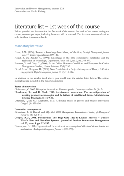
International Research Journal of Applied and Basic Sciences
© 2015 Available online at www.irjabs.com
ISSN 2251-838X / Vol, 9 (3): 418-426
Science Explorer Publications
A Function-Based Image Binarization based on
Histogram
Hamid Sheikhveisi
Payam e Noor University, Zahedan, Iran.
Corresponding Author email:[email protected]
ABSTRACT: A gray-level histogram of an image can be divided into four identical parts of gray-level
value for better operations; our new approach is figured for the correct automatic binarization of
digital images based on the presented theory. The algorithm follows a simple and accurate
synthesis. A rectangular mixture function is employed to multiply by the input image; in this condition,
the function is multiplied to the peak points of the image histogram, and in order to several peak
points in the areas, to have a unity peak point, the global maximum theory is used. Finally achieved
results are compared by ordinary methods: Otsu, Kapur, Rosin and Du algorithms. Experimental
results show the good performance of the new approach toward the others.
Keywords: Segmentation, Image binarization, Gray level image, Histogram, Rectangular function,
Global maximum, Symmetry.
INTRODUCTION
Image segmentation is necessary to image processing and pattern recognition which leads to the high
quality of the final result of analysis. Image segmentation is a process of separating an image into different
regions. One of the particular types of segmentation is thresholding (R. C. Gonzalez et al., 2009); thresholding
is a very low-level image segmentation method. It is widely used as a pre-processing step. One of the more
significant steps in is finding a proper threshold value to segment an arbitrary object from its background. The
next step is maybe defect detections, or any other operations. In more applications, image segmentation is
included in the main step (K. S. Fu and J. K. Mui, 1981; N. R. Pal and S. K. Pal, 1993; P. K. Sahoo, 1988; M.
Sezgin, B. Sankur, 2004). The main idea is that the intensity values of object pixels and the background pixels
differ, such that object and background can be separated by selecting a proper threshold. A binary image is
then obtained by assigning pixels with values less than threshold with zeros and the remaining pixels with ones.
This type of thresholding is called bi-level threshold. We have also another type of thresholding that is proper
for the composed or several distinct objects. In this type of thresholding, a multiple thresholding is applied to a
better thresholding; this is called multi-level thresholding.
Ideally, for a bi-level image, the histogram consists of two peak points; in this condition, the point
between and at the bottommost point of these two peaks (valley), denotes the thresholding point. The optimum
point is gotten into the bottommost one. In this situation, the pixels with less value than this will return to zero
and the pixels that are equal to or bigger than it will return to one (M. Sezgin, B. Sankur, 2004). Let us consider
image f of size M×N with L gray levels in the range [0, L-1]. The gray level or the brightness of a pixel with
coordinates (i, j ) is denoted by f (i, j ) . The threshold T is a value in the range of [0, L-1]. Now the thresholding
technique determines an optimal value for T based on predefined measurements, so that:
1
g (i, j )  
0
for
for
f (i, j )  T
f (i, j )  T
(1)
Where g (i, j ) is binarized image. An example for gray level image, gray level distribution histogram and the
threshold are shown in fig.1.
Intl. Res. J. Appl. Basic. Sci. Vol., 9 (3), 418-426, 2015
16000
14000
12000
10000
Background
Object
8000
6000
4000
2000
0
0
50
100
150
200
250
Figure. 1. Histogram of a gray level image
In the last three decades several methods have been proposed, which set the thresholds according to
a certain criterion, an overview can be found in (M. Sezgin, B. Sankur, 2004).
Typically, there are two approaches for thresholding methods; local and global. In global thresholding,
a same threshold value is used across the whole image. While in local thresholding, an image is separated into
many sub-regions (H.D. Cheng, Y.H. Chen, 1996).
Local thresholding investigates the relationship between brightness of neighborhood pixels to adapt the
threshold in order to the intensity statistic of different. One of the principal drawbacks of local threshold is
finding more than one threshold value in some conditions; the other is the more elapsed time toward global
thresholding. Some factors affect the certain value of gray level and make the threshold get complicated; poor
contrast, inconsistency between sizes of object and background, non-uniformity in the background, and
correlated noise are some of these cases. Since, the prosperity of thresholding depends on the proper
selection of threshold value. In order to the properties the thresholding techniques are employing, sezgin has
categorized them into six groups as below (M. Sezgin, B. Sankur, 2004):
Histogram shape-based methods where the histogram of the image is viewed as a mixture of two Gaussian
distributions associated to the object and back ground classed; Zhi thresholding (Zhi-Kai Huang, Kwok-Wing
Chau, 2008) or sezan thresholding (M.I. Sezan, 1985) are two examples of this method.
Clustering-based methods where the gray level pixels are clustered in two classes as background and
foreground objects, or alternatively modelled as a mixture of two Gaussians; iterative thresholding (T. W. Ridler,
and S. Calvard, 1979), Otsu thresholding (N. Otsu, 1979), minimum error thresholding (J. Kittler and J.
Illingworth, 1986), fuzzy clustering thresholding (D.Mangamma, 2011).
Entropy-based methods use the difference in entropy between the foreground and background regions, such
as Kapur thresholding (J.N. Kapur, 1985) and Peng method (Peng-Yeng Yin, 2002).
Object attribute-based methods find a measure of similarity (fuzzy shape similarity, edge coincidence, etc.)
between the gray level and threshold image; such as edge field matching threshold (L.Herts and R. W. Schafer,
1988) and topological stable-state thresholding (A. Pikaz and A. Averbuch, 1996).
Spatial Methods used higher order probability distribution and/or correlation between pixels such as Brink
thresholding (Brink, A.D., 2002).
Local Methods like san threshold have not good results in order to described drawbacks (Berrin A., 2008).
The proposed method is perfectly independent from thresholding approaches. It defines the binarized
image by multiplying the maximum gray level of the image with the complex rectangular image whereas other
binarization methods just select the proper value for histogram thresholding.
Proposed Approach
The main idea of the proposed approach derived from the gray scale histogram processing; indeed if
we have the maximum value of the intensity histogram (we called it mvih), the histogram diagram is divided to 4
areas. Fig.2 shows an illustration of defined separated.
From fig.2, Area I contains the maximum values of the histogram, while Area IV has the minimum values.
Results from the last literatures showed that if we find two proper peaks and also the suitable valley between
them, a good result can be achieved for thresholding purposes.
419
Intl. Res. J. Appl. Basic. Sci. Vol., 9 (3), 418-426, 2015
Figure. 2. Histogram dividing.
For this approach, mixture rectangular functions are considered to multiply by the input image. Our idea
in this approach is in to find a 0 and/or 1 (binary) function to multiply by the input image for attaining a binary
output image. The presented mixture function is a rectangular function; the rectangle function Π (x) is a function
which is 0 outside the interval [-1/2, 1/2] and unity inside it. It is also called the gate function, pulse function, or
window function, and is defined as (Weisstein, Eric W., 2011):
1

 0 for x  2
 1
1
 ( x)  
for x 
(2)
2
2
 1 for x  1

2
Total procedure for the proposed method is as below:
Step 1) Image acquisition
Step 2) intensity level converting (we consider that the input image is RGB)
The separate values of the three color channels (R, G, and B) are combined to produce an intensity image
(gray) using a commonly accepted transformation as below:
Intensity  0.2989  R + 0.5870  G + 0.1140  B
(3)
If the input image is an intensity level image, step 2 will be neglected.
Step 3) Find the histogram (probability distribution function) of the gray level image; the histogram of a digital
image with L total possible intensity levels in the interval [0, L-1] is defined as the discrete function:
(4)
h[rk ]  nk
th
where rk is the k intensity level in the range [0, L-1] and nk is the number of pixels in the image whose intensity
image is rk. The value of L-1 is also differing for various classes (255 for unit8, 1 for double, etc.).
Step 4) Divide the input histogram to 4 identical areas; fig.3 obviously shows the same dividing between 4
areas.
Step 5) Find the Maximum Points (Peaks) of each area; peak value of whole 4 areas has been found as c1, c2,
c3 and c4. Red points in fig.3 shows the peak values found by the implemented approach.
As it can be seen from fig.3, some problems are made by this method; each 4 areas have more than 1 peak
point. Indeed, local maxima points of each area are extracted. For attaining just 1 peak point for each area, we
need to find the global maxima. A function has a global (or absolute) maximum point at x ∗ if f(x∗) ≥ f(x) for all x.
A global maximum of f(x) in [0, L-1] is basically the greatest value of f(x) in [0, L-1]. Global maxima in [0, L-1]
will always occur either at the critical points of f(x) within [0, L-1] or at the end points of the interval (Thomas,
2010). Three main steps to find the global maxima are as:
Find out all the critical points of f(x) in [0, L-1]. Let l1, l2 …ln be the different critical points.
Find the value of the function at these critical points and also at the end points of the domain. Let the values of
the function at critical points be f (l1), f (l2)………..f (ln).
420
Intl. Res. J. Appl. Basic. Sci. Vol., 9 (3), 418-426, 2015
16000
14000
12000
10000
8000
6000
4000
2000
0
0
50
l1
l2
100
l3
150
200
250
ln
Figure. 3. Areas Dividing and finding the peak points for each area; red stars are the peak value of each area.
Find M1 =Max {f (0), f (l1), f (l2)…f (ln), f (L-1)}.
Now M1is the maximum value of f(x) in [0, L-1].
Step 6) Generate 4 rectangular functions by the center of peak points.
(5)
f ( x)  h(( x  ci ) / b)
where h is height, c is the center, and b is the full-width. h is one in this work, and c is the peak point of areas; b
is calculated as L/32.5 after some trial and errors.
Step 7) Multiply the generated function by the intensity image to get the output binary image.
y   ( x)  I ( x)
(6)
where I and y are pixels in the input (intensity) and output (binary) image, respectively. Fig. 4 shows the result
of the algorithm for an image.
Figure. 4. Multiply of rectangular function and the input image.
Experimental results
We tested the proposed real-time thresholding technique on a Pentium 4 processor at core 2
duo1.60Ghz under Matlab environment (Mathworks, 2010). An experimental test images have been prepared
by complex different dataset to cover a variety of situations and conditions. Some examples of our thresholding
result are shown below.
421
Intl. Res. J. Appl. Basic. Sci. Vol., 9 (3), 418-426, 2015
(A)
(B)
(C)
(A)
(B)
(C)
(A)
(B)
(C)
422
Intl. Res. J. Appl. Basic. Sci. Vol., 9 (3), 418-426, 2015
(A)
(B)
(C)
(A)
(B)
(C)
(A)
(B)
(C)
Figure. 5. (A) Original image with different sizes, (B) Histogram (Probability Distribution) of the input image, (C) Binarized
image.
The experiment result of proposed approach is then compared by Otsu, Kapur method (J.N. Kapur et
al., 1985) and local relative entropy threshold (LRE), joint relative entropy threshold (JRE) and global relative
entropy threshold (GRE) (Y. Du, 2004); we are also used Rosin method (Venkatesh, S. and P. Rosin., 1995),
but in order to improper results, it is neglected in evaluation section. To evaluate the performance of the
proposed algorithm toward the other conditional methods, six performance metrics are defined:
TP
TP  FN
TN
Specificity 
TN  FP
(7)
TP
TP  FP
TN
Negative. Pr edictive.Value 
TN  FN
TP  FP
Index.of .Suspicion 
TP  FN
TP
Diagnostic. Accuracy 
TP  FP  FN
(9)
Sensitivity 
Positive. Pr edictive.Value 
(8)
(10)
(11)
(12)
where TP is the number of true positives, FN the number of false negatives, TN the number of true
negatives, and FP the number of false positives. A positive is a part that is classified as object; true
classification is defined by an expert. The sensitivity and specificity measure the percentages of accurate
classifications for the object and background cases, respectively. The positive predictive value is the proportion
of object classified as object that is really object, and inversely for the negative predictive value. The index of
suspicion gives the degree of awareness of the likelihood of an object to be an object. An index higher than
100% represents an over-diagnosis while an index lower than 100% represents under-diagnosis. The diagnosis
423
Intl. Res. J. Appl. Basic. Sci. Vol., 9 (3), 418-426, 2015
accuracy shows the loss of accuracy due to misclassified elements. Table 1 shows the different classification
accuracy indices for three combinations of segmentations: Proposed method, Otsu, Kapur, LRE, JRE and
GRE.
Table.1. Segmentation symmetry values for image binarization
Symmetry Features
Sensitivity (%)
Specificity (%)
Positive predictive value (%)
Negative predictive value (%)
Index of suspicion (%)
Diagnostic accuracy (%)
Proposed
81
16
51
43
157
46
Otsu[22]
71
26
52
45
138
43
Kapur [23]
63
75
63
23
100
46
LRE [24]
57
40
52
47
110
37
(A)
(B)
(C)
`
(D)
(E)
(F)
(G)
(H)
(I)
JRE [24]
42
62
62
42
122
33
GRE[24]
56
45
45
56
112
33
Figure. 6. Results of thresholding of images from the difference dataset with various algorithms; (A) Input image, (B)
Histogram of the image, (C) Otsu, (D) Kapur, (E) Rosin, (F) LRE, (G) JRE and (H) GRE thresholding.
(A)
(B)
(C)
424
Intl. Res. J. Appl. Basic. Sci. Vol., 9 (3), 418-426, 2015
(D)
(E)
(F)
(G)
(H)
(I)
Figure. 7. Results of thresholding of images from the difference dataset with various algorithms; (A) Input image, (B)
Histogram of the image, (C) Otsu, (D) Kapur, (E) Rosin, (F) LRE, (G) JRE and (H) GRE thresholding.
(A)
(B)
(C)
(D)
(E)
(F)
(G)
(H)
(I)
Figure. 8. Results of thresholding of images from the difference dataset with various algorithms; (A) Input image, (B)
Histogram of the image, (C) Otsu, (D) Kapur, (E) Rosin, (F) LRE, (G) JRE and (H) GRE thresholding.
CONCLUSIONS
In this paper, a novel gray level binarization algorithm is proposed using the rectangular function. In order
to the fact that the histogram of image can be used to depict the statistical character of probability density
function, the peak points of histogram is used to find the proper point of binarization. A rectangular function is
used to achieve the proper function which gets 1 for some defined peak points and inverse, gets zero for less
value points respectively. As an example of the application of the methodology, tests were performed on a
random selection of different dataset providing a quantitative and thorough evaluation of six different
425
Intl. Res. J. Appl. Basic. Sci. Vol., 9 (3), 418-426, 2015
thresholding algorithms. The final conclusion is that using the function-based system outperforms the other
conditional approaches.
REFERENCES
Berrin A. Yanikoglu, Berkner K.2008. "Efficient implementation of local adaptive thresholding techniques using integral images", Proc. SPIE
6815, 681510,
Brink, AD. 2002."Minimum spatial entropy threshold selection ", Vision, Image and Signal Processing, IEE Proceedings, vol.142, pp.128132
Cheng HD, Chen YH.1999. "Fuzzy Partition of Two-Dimensional Histogram and its Application to Thresholding", Pattern Recognition,
vol.32, pp.825-843,
Du Y, Chang C, Thouin PD.2004. "An Unsupervised Approach to Color Video Thresholding", Optical Engineering, vol. 43, No. 2, 282-289,
Fu KS, Mui JK. 1981. "A Survey on Image segmentation", Pattern Recognition, vol.13, pp.3-16, Pergamon Press Ltd, Oxford
Gonzalez RC, Woods RE, Eddins SL. 2009.Digital Image Processing. Gatesmark Publishing Company,
Herts L, Schafer RW. 1988. "Multilevel Thresholding Using Edge Matching", Computer Vision Graphic Image Processing, vol.44, pp.279295
Kapur JN, Sahoo PK, Wong AKC. 1985. "A new method for gray level picture thresholding using the entropy of the histogram", Comput.
Vis. Graph. Image Process. vol.29, pp.273–285
Kapur JN, Sahoo PK, Wong AKC.1985. "A new method for gray level picture thresholding using the entropy of the histogram", Comput.
Vis. Graph. Image Process. vol.29, pp.273–285
Kittler J, Illingworth J. 1986."Minimum Error Thresholding", Pattern Recognition, vol.19, pp.41-47
Mangamma D, Nanaji U, Nagaragu C, Veni N. 2011."Implementation of object oriented approach to Automatic Histogram Threshold based
on Fuzzy Measures", International Journal of Engineering Research and Applications (IJERA), vol. 1, Issue 4, pp. 1623-1628,
Matlab Tutorial, Mathworks, 2010.
Otsu N.1979."A threshold selection method from gray-level histograms". IEEE Transactions on Systems, Man and Cybernetics, vol. 9, No.
1, pp. 62-66
Pal NR, Pal SK. 1993."A Review on Image Segmentation Techniques", Pattern Recognition, Elsevier, vol. 26, No. 9, pp. 1277-1294,
Killington,
Peng-Yeng Y.2002."Maximum entropy-based optimal threshold selection using deterministic reinforcement learning with controlled
randomization", Signal Processing, vol.82, pp.993-1006
Pikaz A, Averbuch A. 1996. "Digital Image Thresholding Based on Topological Stable State", Pattern Recognition, vol.29, pp.829-843,
Ridler TW, Calvard S. 1979. "Picture Thresholding Using an Iterative Selection Method", Systems Man and Cybernetics, SMC-8, pp.630632
Sahoo PK, Soltani S, Wong AKC. 1988."A Survey of Thresholding Techniques", Computer Vision, Graphics, and Image Processing, vol.
41, 133-260, Canada,
Sezan MI.1985. "A Peak Detection Algorithm and Its Application to Histogram-Based Image Data Reduction", Graphic Models and Image
Processing, vol.29, pp.47-59,
Sezgin M, Sankur B. 2004. "Survey over image thresholding techniques and quantitative performance evaluation", Journal of Electronic
Imaging, vol.13 (1), pp.146-165, Istanbul,
Thomas George B, Weir Maurice D, Hass J. 2010.Thomas' Calculus: Early Transcendentals (12th ed.). Addison-Wesley. ISBN: 0-32158876-2,
Venkatesh S, Rosin P. 1995. "Dynamic threshold determination by local and global edge evaluation". Computer Vision, Graphics and Image
Processing, vol.57 (2), pp.146–160
Weisstein Eric W. 2011."Rectangle Function". http://mathworld.wolfram.com/RectangleFunction.html, 15 August
Zhi-Kai H, Kwok-Wing Ch. 2008."A New Image Thresholding Method Based on Gaussian Mixture Model", Applied Mathematics and
Computation, vol. 205, No. 2, pp. 899-907
426