Download Report

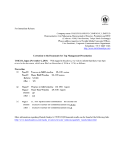
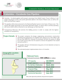
Comprehensive data reduction package for the Immersion
GRating INfrared Spectrograph: IGRINS
Chae Kyung Sima , Huynh Anh Nguyen Lea , Soojong Paka,∗, Hye-In Leea , Wonseok
Kangb , Moo-Young Chunc , Ueejeong Jeongc , In-Soo Yukc , Kang-Min Kimc , Chan
Parkc , Michael D. Paveld , Daniel T. Jaffed
a Kyung Hee University
1732 Deogyeong-daero, Giheung-gu, Yongin-si, Gyeonggi-do, 446-701, Korea
b National Youth Space Center
200 Deokheungyangjjok-gil, Dongil-myeon, Goheung-gun, Jeollanam-do, 548-951, Korea
c Korea Astronomy and Space Science Institute
776 Daedeokdae-ro, Yuseong-gu, Daejeon, 305-348, Korea
d University of Texas at Austin, 2515 Speedway, Stop C1400, Austin, TX 78712, U.S.A.
Abstract
We present a Python-based data reduction pipeline package (PLP) for the Immersion
GRating INfrared Spectrograph (IGRINS), an instrument that covers the complete Hand K-bands in one exposure with a spectral resolving power of 40, 000. The reduction
steps carried out by the PLP include flat-fielding, background removal, order extraction, distortion correction, wavelength calibration, and telluric correction using spectra
of A type standard stars. As the spectrograph has no moving parts, the PLP automatically reduces the data using predefined functions for the processes of order extraction,
distortion correction, and wavelength calibration. Before the telluric correction of the
target spectra, the intrinsic hydrogen absorption features of the standard A star are removed with a Gaussian fitting algorithm. The final result is the flux of the target as
a function of wavelength. Users can customize the predefined functions for the extraction of the spectrum from the echellogram and adjust the parameters for the fitting
functions for the spectra of celestial objects, using ‘fine-tuning’ options, as necessary.
Presently, the PLP produces the best results for point-source targets.
Keywords: methods: data analysis, techniques: spectroscopic
1. Introduction
IGRINS (Immersion GRating INfrared Spectrograph) is a cross-dispersed nearinfrared spectrograph that uses a silicon immersion echelle grating as its main dispersing element. It covers all of the H- and K-bands in a single exposure with a resolving power of R = λ/∆λ ∼ 40, 000. The H- and K-bands echellograms consist of
∗ Corresponding
author
Email addresses: [email protected] (Chae Kyung Sim), [email protected] (Soojong Pak)
Preprint submitted to Advances in Space Research
April 6, 2015
23 and 20 orders, respectively (Figure 1). Since the spectrograph has no moving parts,
the transformation functions for the order extraction, distortion correction, and wavelength calibration vary very little from one exposure to the next. Hence, a deliberately
designed pipeline is to provide stable quality of data reduction process with minimal
human intervention.
[Figure 1]
The full IGRINS hardware and software system is described earlier (Yuk et al.,
2010). The IGRINS software consists of six packages to be used before, in the middle
of, and after the observation. To prepare the observation, one can use the Exposure
Time Calulator (ETC) and a finding-chart produced with the Observational Preparation
Package (OPP). During the observation, Housekeeping Package (HKP), Slit Camera
Package (SCP), Data Taking Package (DTP), and Quick Look Package (QLP) conduct
the observation. Afterwards, the data can be reduced by the Pipeline Package (PLP).
This package can also be used during the night to help the observer to decide further
observation strategies. A diagram of the overall configuration of the IGRINS system is
shown in Figure 2.
[Figure 2]
The PLP reduces the IGRINS data following the well-estabilished procedure for
reduction of echellogram images: flat-fielding, background removal, order extraction,
distortion correction, wavelength calibration, and telluric correction. As the spectrograph has no moving parts, the functions to represent the echellogram mapping are
theoretically defined. The reduction processes of order extraction, distortion correction, and wavelength calibration can be run in an automated way using the predefined
functions. The functions can then be revised in a “fine tuning” mode that interacts with
the user during the run.
To make use of the PLP, the observer should follow the standard observing sequences which requires assigning reduction group number to each echellogram, observing A0V type standard star, and using “Nod-on-Slit” mode for the stellar objects.
In the following sections, we write about the PLP from the standpoint of its architecture in § 2, describe the standard observing sequence for IGRINS in § 3, illustrate the
detailed reduction process of the pipeline in § 4, and summarize in § 5. The“pipeline”
hereafter refers to the PLP of the IGRINS software.
2. Architecture of the IGRINS Pipeline
All of the IGRINS software including the pipeline is written in Python1 2.7, which
is freely available for many platforms including Microsoft Windows, Mac OS, and
linux systems. In addition to its straightforward syntax and intuitive graphical user
interface, the advantage of python as an astronomical tool lies in its extensibility to
many scientific algorithms using the wide variety of available open-source libraries
(Greenfield, 2011; Robitaille et al., 2013).
The pipeline, developed in the Mac OS 10.8, has been tested in Mac OS 10.79, Microsoft Windows XP and 7, CentOS 5.9 and Ubuntu 10.4.4. It makes use of
1 http://www.python.org/
2
scientific, astronomical, and graphical libraries such as NumPy2 , SciPy3 , PyFits4 ,
matplotlib5 . It also works with NumPy 1.6-8, SciPy 0.12-13, PyFits 3.0-1,
and matplotlib 1.1-4. One potential limitation for users running the pipeline at
their home institutions is the occurrence of memory error in some cases of operation
with a 32-bit OS, mainly due to the large size of the IGRINS 2K×2K array detector
and hence those of FITS files.
During the observing night, raw echellograms are saved as FITS files and an ASCIIformatted observation log is saved to the storage via Data Taking Package (DTP). The
pipeline makes use of the log to categorize echellograms into dark, flat, arc, standard,
and target. At every step of the reduction process, reduced echellograms and spectra
are saved as FITS files. The final result is intensity versus wavelehgths spectrum for
each order of the echellogram.
To help users check intermediate stages, additional images displaying the spectra of
wavelength calibration and telluric correction processes are saved in the PNG format.
Description of each process is displayed in the Python console window and the same
content is saved into a reduction log. The current pipeline version and system time at
the start and the end of the run is also saved into the log file. The reduction history, i.e.,
metadata, for each FITS file is saved in its header.
The software code, installation guide, and user’s manual will be provided via web6
in early 2014.
3. Standard Observing Sequence
To make use of the pipeline, the observer should abtain data using the IGRINS
standard observing sequence. In short, a star-like point source target and an A-type star
as a telluric standard should be observed using “Nod-on-Slit” mode and every frame
should have its own “Group ID” assigned.
The rationale for selecting A-type stars as standards is that their H- and K-band
spectra contain intrinsic lines that are ignorable or easily removed (Vacca et al., 2003).
There are few metal lines whose strengths are only few percent of the continuum
and photospheric hydrogen lines whose spectral profiles are almost Gaussian. As the
pipeline automatically fits and removes the hydrogen lines from the spectra of standard star frames (see 4.3.1), observing A stars as standard is preferable. Details on the
“Nod-on-Slit” mode and “Group ID” are given in the following subsections.
3.1. “Nod-on-Slit” Mode Observation
The observed data number (DN) is a sum of dark current, telescope and sky background, as well as the target signal. As the background is a significant source of radiation in the near-infrared, nodding is one general strategy to effectively remove the
2 http://www.numpy.org
3 http://www.scipy.org/
4 http://www.stsci.edu/institute/software
hardware/pyfits
5 http://www.matplotlib.org
6 http://irlab.khu.ac.kr/∼igrins/
3
backgrounds. When an exposure on the celestial object (A frame) is followed by equal
time of exposure on the nearby sky background (B frame), subtracting the B frame
from the A frame effectively removes the sky background as well as dark current and
telescope background (e.g., Cushing et al., 2004).
The Data Taking Package (DTP), the control software for the spectrograph and calibration system of IGRINS, provides the observing modes for a celestial object. One
is “Stare” mode that keeps the star at the center of the slit. It will be used to confirm
whether the telescope is properly pointing the target and to determine the object’s position inside the slit. Another one is “Nod-on-Slit” mode that nods the telescope so
that the star is at right and left by turns inside the slit. “Nod-off-Slit” mode also nods
the telescope but keeps star and nearby blank sky at the center of the slit in rotation.
Among them, “Nod-on-Slit” mode is most likely to be preferred because it reduces the
total observing time and averaging A and B frames increases the signal-to-noise ratio
of the spectrum when the target is a point source. When observing extended sources
such as planets, interstellar clouds, and galaxies whose angular size is comparable to
or larger than the slit length, “Nod-off-Slit” mode is a good alternative.
Reduction processes for extended sources cannot be easily generalized into a single
sequence since the reduction procedure varies of the object, its size relative to that of the
slit, observing mode (staring or scanning), and the method to remove the background
sky feature. In its automated mode, the pipeline only deals with IGRINS data obtained
in “Nod-on-Slit” mode.
To be compatible with A and B frames for celestial objects, halogen lamp data
should be obtained as a pair of ON and OFF frames. Subtracting the OFF frame from
the ON frame removes dark current and telescope backgrounds as the nod-and-subtract
strategy does.
3.2. Assignment of the “Reduction Group”
For those who observe many point source targets in a single night using on-slit
nodding, the pipeline categorizes the obtained frames by “Group ID”. The observer
designates the “Group ID” for each frame using the DTP. Consecutive frames with the
same “Group ID” are regarded as a group and the pipeline carries out the reduction
separately for each group. Frames in one group share the same calibration data. A
standard star needs to be at similar air-mass as the target. In general, each group may
last for 1−3 hours of the observing night.
“Group ID” consists of two numbers. A frame that is to be used in only one reduction group ought to has two identical numbers (e.g., 1 and 1) as its “Group ID”. In case
of a calibration frame that is to be used for both of the two sequential groups, observer
can assign two different numbers (e.g., 1 and 2). Then the pipeline uses those frames
for reductions of both groups. An example of the standard observing sequence using
‘’Nod-on-Slit” mode is shown in Table 1.
[Table 1]
4. Reduction Process
The pipeline serves to transform the raw IGRINS echellograms of astronomical
targets and their associated calibration frames into spectra of relative intensity ver4
sus wavelength on the basis of the observational log (written by Data Taking Package
(DTP)). In terms of its functional aspects as well as the running-time, the pipeline
serves in two modes:
◦ fast mode works within a few minutes to give the observer at the telescope an
idea of the science quality of the data, to be used in the observation night;
◦ fine-tuning mode interacts with the user to review the intermediate results and to
fine-tune the reduction processes.
Though several options for the fine-tuning mode are separated in the detailed process inside the pipeline, they are blended from the user’s point of view. In the graphical
user interface (Figure 3), the pipeline is divided into three parts as follows:
◦ Preparations − Selection and categorization of the frames to be reduced making
use of observing log.
◦ Calibration data reduction − Pre-processing of the frames of dark current, halogen lamps, arc lamps, and derivation of the transformation functions for order
extraction, distortion correction, and wavelength calibration.
◦ Object data reduction − Pre-processsing, order extraction, distortion correction,
wavelength calibration of the frames of standard stars and target objects, hydrogen line removal from the standards, and telluric correction of the targets.
We describe each part of the process in sections §§ 4.1−4.3. To discriminate observation data, we adopt a few notations; [ttt] stands for the exposure time, [ii] for
the sequential number under the fixed observation parameters, and [jj] for the order
number of the extracted strips from the echellogram. If the observer has assigned two
or more Group IDs (see §§ 3.2), the pipeline repeats the entire processing for each
reduction group. The process of one group is illustrated in Figure 4.
[Figure 4]
The basic algorithms that are shared for two or more different types of frames appears only once. The methods to correct bad pixels and to combine echellograms are
presented in §§§ 4.2.1. Cosmic-ray correction is described in §§§ 4.3.1.
4.1. Preparation of Frames for Reduction
Making use of the observation log written by the DTP during the observation, the
pipeline reads the file list and automatically categorizes the data files by their type, i.e.,
dark current, flat field, arc, standard, and target. The names of the classified files appear
in a listbox. When the user marks some files in a listbox, only those file are reduced.
Files should be marked as a pair of ON and OFF or A and B files for calibration or
object data, respectively.
4.2. Calibration Data Reduction
4.2.1. Dark
Dark frames that are observed and corrected for the bad-pixels (if requested) with
several different exposure times [ttt], dark[ttt] [ii], are combined to make DARK[ttt]
and saved. The number of saved DARK files is determined by the number of different
exposure times.
5
Bad pixel correction is done when requested, The bad-pixel positions in the observed echellogram image are designated by using a pre-defined mask image. Bad
pixels are replaced using a linear interpolation of the two nearest-neighbor good pixels
(in lines or columns).
Combining algorithm computes either median or average value of echellograms
on a pixel-by-pixel basis. Sigma clipping is one option that ignore pixel values that
deviate more than the input value on GUI multiplied by the standard deviation.
4.2.2. Flat and Order Extraction Map
It is required to take exposures with the halogen lamp on and off as a set. The
observed (and corrected for bad-pixels as described in §§§ 4.2.1, when requested)
flat on [ii] and flat off [ii] images are combined to make flat on and flat off,
respectively. Subtracting the flat off from the flat on on a pixel-by-pixel basis
makes the difference frame, flat onoff.
The pipeline scales the pixel values of flat onoff so as to set the median value
to unity to facilitate the estimation of the signal-to-noise ratio (S/N) of the spectra of
celestial objects afterwards. The normalized flat image is saved as FLAT.
In addition to its use in flat-fielding, the high S/N flat image is essential for the
determination of the position of the echellogram orders (Cushing et al., 2004). The
pipeline makes use of an edge detection algorithm to find the order locations. At the
center column of the echellogram (center of the spectral direction axis), the gradient
of the cross-cut flux f along the spatial direction is the first order numerical derivative
(Starck & Murtagh, 2006; Gonz´alez et al., 2002; Jain, 1989):
fy =
∂f
,
∂y
(1)
where y is the pixel positions along the spatial direction.
The pixel positions where the derivatives have positive and negative peaks are the
upper and lower edges, respectively, of orders in the echellogram (Figure 5). The
pipeline repeats the edge detection for columns of every 40 other pixels along the abscissa and fits the edge positions of each order with a septic function:
y = a0 + a1 x + a2 x2 + . . . + a7 x7
(2)
where x is the pixel position along the spectral direction.
[Figure 5]
An order extraction map refers to an ASCII file that contains the coefficients table
for all orders. It is saved to a designated folder in storage for the spectral extraction
process afterwards. Once saved, the map can be used whenever needed and thus saves
computing time. For this purpose, the “Standard Transformation Functions”, predefined order extraction map and distortion correction functions (see §§§ 4.2.3), will be
distributed along with the software. The fast mode (see § 4) of the pipeline as well as
the Quick Look Package (QLP) utilizes the “Standard Transformation Functions”. The
fine-tuning process, i.e., reviewing of the extraction result and/or customizing the map
or switching it to another one previously customized, can be done upon request in the
GUI.
6
In the fine-tuning mode, the pipeline displays the differences between the current
extraction map and that derived by the edge detection algorithm. Figure 7 shows one
example; residuals of pixel positions in the upper and lower edges when the standard
map is used. When closing the residual display, the user is asked to decide whether to
update the extraction map.
[Figure 7]
From the Flat image, orders are extracted using the extraction map defined above.
When rectifying the curved orders, the pixels move only along the ordinate (spatial
direction axis) by an integer-number of pixels to preserve the observed data number
(DN) without interpolation. Extracted strips are saved to storage as FLAT [jj].
4.2.3. Arc and Distortion Correction Function
Similarly to the flat frame processing in §§§ 4.2.2, the observed (and corrected
for bad-pixels upon request) echellograms with the arc lamp on and off, arc on [ii]
and arc off [ii], are combined to make arc on and arc off, respectively. Subtracting arc off from arc on on a pixel-by-pixel basis makes the difference frame,
arc onoff. To extract orders from the arc image, the same extraction map used in the
flat frame processing is used. Extracted strips are saved as ARC [jj] in storage.
Arc frames are used to correct the distortion in the spectral direction of the extracted
orders. The pipeline finds emission features for several rows along the ordinate (spatial
direction axis) and fit the features with a second order polynomial to make the distorted
spectral lines straight. The pixel value moves only in abscissa (spectral direction axis)
at this time and the observed DN are preserved without interpolations. Comparing the
straghtened emission features to the arc line list enveloped in the software, the pipeline
transform the rectified strip into the wavelength-calibrated one. Figure 8 shows before
and after the transformation.
[Figure 8]
To ensure the quality of the rectification and wavelength registration, every order
should have several spectral lines of the arc lamp and the lines should be widely distributed along the spectral direction in an order, which is not the case of several orders
of IGRINS echellogram. One good substitute for the arc lamp is the emission lines of
the night sky. For the sake of the OH lines that are bright, numerous, and diversely
distributed at most of the orders of H- and K- band (Rousselot et al., 2000). To use OH
lines as arc, one is to add the sky frame into the arc list on the GUI. The pipeline will
select appropriate lines in its enclosed database that consists of ThAr and UNe lamp
lines and OH lines on the basis of the target name field in the observation log.
As briefly mentioned in §§§ 4.2.2, the distortion correction function and the order
extraction map makes “Standard Transformation Functions”. As fine-tuning processes,
result-viewing of the distortion correction and wavelength calibration and/or correcting
or switching the functions can be done upon request in the GUI.
4.3. Object Data Reduction
Here we describe the process of the A-type standard star and a star-like point source
target that are observed in the “Nod-on-Slit” mode as illustrated in § 3.
7
4.3.1. Standard Star and Telluric Correction Spectra
The observed std A [ii] and std B [ii] images are corrected for bad-pixels and
for cosmic rays upon request in the GUI. The bad-pixel correction method is the same
as described earlier in §§§ 4.2.1.
Cosmic ray correction is done by detecting the pixels with brighter flux than a
threshold value of flux = 1, 000 in analog-digital units (ADU). When the candidate pixels are marked, the ratio of the median value of the 8 surrounding good pixels (within
the window of 3 × 3) to the marked pixel is computed. If the calculated ratio is lower
than the flux-ratio threshold of 0.2 , then the value of the marked pixel is replaced by the
median value of the 8 surrounding good pixels. We note that the flux-ratio threshold of
0.2 is from heuristics during the development stage and is subject to change when the
real observation test is available in the early 2014, before distribution of the pipeline.
For each pair of A and B frames, subtracting the std B [ii] frames from the corresponding std A [ii] frames in order makes the difference images, std AB [ii],
that are free from dark currents and sky and telescope background. After dividing
the difference images by the normalized FLAT, the pipeline combines the flat-fielded
std AB [ii] and save to storage. The number of the combined images are determined
by the number of standard stars observed in a “Reduction Group”.
Then the pipeline extracts the orders, correct the distortions, and register wavelenthsn to make STD [jj] using the “Standard Transformation Functions” or other
ones that is determined in the most recent calibration data processing or specified directly in the GUI by the user.
Now each order strip consists of a positive A spectral signal and a negative B signal (Figure 6). To extract both of them excluding the background, the pipeline uses
the sum of the cross-cuts. The rows within the full-width at half-maximum (FWHM)
of each stellar feature. Then the pipeline accumulates the the pixel values along the
ordinate (spectral direction axis) to make a positive A (STD tp [jj]) and a negative B (STD tp [jj]). Averaging STD tp [jj] (A) and −STD tn [jj] (−B) yields
STD tpn [jj], spectra of the standard star with an increased S/N.
[Figure 6]
Spectra of A-type stars can be used for telluric line correction of the stellar A stars
have very few absorption features in the near-infrared (Vacca et al., 2003). The A star
spectra, however, have strong hydrogen absorption lines. Brackett series transitions are
widely distributed in the H-band and the Br-γ and δ lines appear in the K-band.
Removing hydrogen lines is a straightforward process due to their line shape that is
analogous to a Gaussian profile. From the spectra of STD tpn [jj] above, hydrogen
lines are fitted with Gaussian profiles. The first guess on the center wavelengths comes
from the Rydberg formula. Two or more lines in one order are fitted with the sum
of the same number of Gaussians (Gaussian mixture). The continuum of each order
is fitted with a third order polynomial and multiplied with the Gaussian mixture to
provide a proper baseline. While fitting, telluric lines are excluded by sigma clipping.
With iteration, a combination of Gaussian mixture and a polynomial that fits best to
spectrum of each order is attained. Subtracting the Gaussian mixture model from the
STD tpn [jj] makes the intrinsic hydrogen lines to be removed.
The hydrogen-free standard spectra are normalized to make telluric correction specta.
8
Assuming the similar air-mass condition for each group, the pipeline removes the continua of the standard star dividing them with derived polynomials and makes the telluric
correction spectrum (Figure 9). Resulted STANDARD [jj] are saved to storage and to
be used for the telluric correction of the target spectra.
[Figure 9]
4.3.2. Target Star
The processing procedure of the target star is same with standard star case; subtraction B from A, flat-fielding, order extraction, distortion correction, wavelength registration, and average A and A stellar features. Telluric correction process divides the resulted target spectra TAR tpn [jj] by STANDARD [jj], the telluric correction spectra
derived previously in §§§ 4.3.1. That makes the final result, TARGET [jj] (Figure 10).
[Figure 10]
5. Summary
We present a Python-based data reduction pipeline for the Immersion GRating INfrared Spectrograph (IGRINS). The software treats the FITS format data obtained with
the “Nod-on-Slit” observing mode on the basis of the “Reduction Group” assigned during the observation. The pipeline provides high-quality spectra with minimal human
intervention and order extraction, distortion correction, and wavelength calibration can
be automatically carried out using the predefined functions. The optional fine-tuning
mode facilitates reviewing the automated process and modifying the pre-defined transformation functions.
IGRINS will be compatible with telescopes of diameters ranging from 2.7-m (the
Harlan J. Smith telescope at McDonald Observatory) to 8−10 m. Commissioning and
initial operation of the IGRINS will be on the 2.7-m Harlan J. Smith telescope at McDonald Observatory from early 2014. Since IGRINS is a prototype of GMTNIRS,
Giant Magellan Telescope Near-InfraRed Spectrometer (Lee et al., 2010), an extension
of this pipeline will serve as the basis for the GMTNIRS reduction software.
Acknowledgement
H. A. N. Le, S. Pak, and H.-I. Lee are partly supported by Creative Research Initiatives program of the Korea Science and Engineering Foundation (KOSEF), grant
No. 2009-0063616, funded by the Ministry of Education, Science and Technology
(MEST). This work was partially supported by the BK21 plus program through the
National Research Foundation (NRF) funded by the Ministry of Education of Korea.
References
Cushing, M.C., Vacca, W.D., & Rayner, J.T. Spextool: A Spectral Extraction Package
for SpeX, a 0.8-5.5 Micron Cross-Dispersed Spectrograph. Pub. Astron. Soc. Pac.
116, 362-376, doi:10.1086/382907, 2004.
9
Gonz´alez, R.C. & Woods, R.E. Digital image processing, second ed. Prentice Hall,
New Jersy, 2002.
Greenfield, P. What Python Can Do for Astronomy, in: Evans, I.N., Accomazzi A.,
Mink D.J., et al. (Eds.), Astronomical Data Analysis Software and Systems XX,
Astron. Soc. Pac. Conf. Ser., 442, pp.425-433, 2011.
Jain, A.K. Fundamentals of Digital Image Processing, Prentice Hall, New Jersy, 1989.
Lee, S., Yuk, I.S., Lee, H., et al. GMTNIRS (Giant Magellan Telescope near-infrared
spectrograph): design concept, in: Soc. Photo-Optical Instr. Eng. (SPIE) Conf. Ser.,
doi:10.1117/12.857630, 2010.
Robitaille, T.P., Tollerud, E.J., Greenfield, P., et al. Astropy: A community Python
package for astronomy, Astron. & Astrophys., 558, A33, doi:10.1051/00046361/201322068, 2013.
Rousselot, P., Lidman, C., Cuby, J.G., et al. Night-sky spectral atlas of OH emission
lines in the near-infrared, Astron. & Astrophys. 354, 1134-1150, 2000.
Starck, J.L. & Murtagh, F. Astronomical Image and Data Analysis, Springer, Berlin
Heidelberg, doi:10.1007/978-3-540-33025-7, 2006.
Vacca, W.D., Cushing, M.C., & Rayner, J.T. A Method of Correcting NearInfrared Spectra for Telluric Absorption, Pub. Astron. Soc. Pac., 115, 389-409,
doi:10.1086/346193, 2003.
Yuk, I.S., Jaffe, D.T., Barnes, S., et al. Preliminary design of IGRINS (Immersion
GRating INfrared Spectrograph), in: Soc. Photo-Optical Instr. Eng. (SPIE) Conf.
Ser., doi:10.1117/12.856864, 2010.
10
Table 1: Example of the standard observing sequence for “Nod-on-Slit” mode using “Group ID”
Frame Type
Calibration lamp
Standard star 1
Target star 1
Target star 2
Calibration lamp
Target star 3
Target star 4
Standard star 2
Calibration lamp
Target star 5
Target star 6
Standard star 3
Calibration lamp
..
.
Group ID
1, 1
1, 1
1, 1
1, 1
1, 1
1, 1
1, 1
1, 2
1, 2
2, 2
2, 2
2, 2
2, 2
Reduction Process 1
11
Reduction Process 2
Figure 1: Simulated IGRINS H- and K-bands flat echellogram. Echelle order number increases from top to
bottom; wavelength increases from bottom to top and left to right. In each order, the spectral (dispersion)
direction is along the horizontal axis, while the spatial direction is along the vertical axis.
12
Figure 2: System architecture diagram of the IGRINS software.
13
Figure 3: The main GUI of the IGRINS pipeline
14
Figure 4: Pipeline processing procedure. [ttt] stands for the exposure time, [ii] for the sequential
number under the fixed observation parameters, and [jj] for the order number of the extracted strips from
the echellogram.
15
Figure 5: Spatial direction cross-cut of the FLAT at the center column of the spectral direction (upper panel)
and the numerical derivatives of the cross-cut to find the upper and lower edges of each order of the echellogram.
16
Figure 6: An extracted strip of the echellogram showing a positive A and a negative B features (upper panel)
and the summation of that strip along the spectral direction (lower panel). The read lines show pixel range
corresponding to the FWHM for each signal.
17
Figure 7: The residuals of the pixel positions of the upper (blue) and lower (red) edges of extracted strips
from a flat frame using the standard map. The numbers in the abscissa refer to the order. Between the
order numbers are pixel positions in the ordinate (spectral direction axis) of each exracted strip. Scince we
deliberately tilted the flat image by 0.1◦ to test the fine-tuning mode, the residuals in this plot exaggerated
relative to those in the real observation.
18
Figure 8: A strip of IGRINS echellogram before (upper panel) and after (middle panel) the distortion correction and wavelength calibration using night sky OH lines and the resulted spectrum of the strip (lower
panel).
19
Figure 9: An example of simulated standard star spectrum of an order Before (upper panel and After (lower
panel) the H lines and continuum removal. Best fits for the continuum (red) and Gaussian mixture to reproduce the hydrogen lines (green) are also shown. Telluric lines are ignored in fitting by sigma clipping.
20
Figure 10: Example spectra of the final step using simulated echellograms.
21