
Concepts Seeds Gathering and Dataset Updating Algorithm for
الجامعة اإلسالمية – غزة Islamic University – Gaza Deanery of Post Graduate Studies عمــــادة الدراســــــــات العليـــــــــا Faculty of Information Technology كليـــــة تكنولوجيـــــــا المعلومـــــــــــــات برنامج تكنولوجيا المعلومات Program of Information Technology Concepts Seeds Gathering and Dataset Updating Algorithm for Handling Concept Drift By Ibrahim Elbouhissi Supervised By Prof. Nabil M. Hewahi A Thesis Submitted in Partial Fulfillment of the Requirements for the Degree of Master in Information Technology January. 2015 i Abstract Our life does not stop evolving and changing and our systems should be adapted to such behavior. The data mining is considered important and vital tool that helps us to get valuable information from hidden patterns and data. The main task in data mining is learning models. The traditional way for learning is called batch learning, which assumes that all training examples are available at the time of learning. In data mining, the phenomenon of change in data distribution over time is known as concept drift. The traditional classification models do not handle this change. In this research, we introduce a new approach called Concepts Seeds Gathering and Dataset Updating algorithm (CSG-DU) that gives the traditional classification models the ability to adapt and cope with concept drift as time passes. CSG-DU is concerned with discovering new concepts in data stream and its main target is to increase the classification accuracy using any classification model when changes occur in the underlying concepts. Handling concept drift is done by selecting the data instances that represent the new concepts and inject them into the training dataset. Our proposed approach has been tested using synthetic and real datasets that represent different types of concept drift (sudden, gradual and incremental). The experiments conducted show that after applying our approach, the classification accuracy increased from low values to high and acceptable ones. Finally, a comparison study between CSG-DU and Set Formation for Delayed Labeling algorithm (SFDL) has been conducted; SFDL is an approach that handles sudden and gradual concept drift. Results indicate that our proposed approach outperforms SFDL in terms of classification accuracy. Keywords: Data Mining, Concept Drift, Machine learning, Concept Drift Detection, Data Stream Mining, Classification. ii عنوان البحث: خوارزمية جمع بذور المفاهيم وتحديث مجموعة البيانات لمعالجة تغير المفهوم ملخص: حياتنا ال تتوقف في تطورها وتغيرها وال بد من جعل أنظمتنا وبرامجنا تتكيف وتتالءم مع طبيعة هذا التغير والتطور .في اآلونة األخيرة ،يعتبر التنقيب عن البيانات أداة مهمة وحيوية في المساعدة على الحصول على معلومات مفيدة من أنماط البيانات المخفية والبيانات المخزنة مسبقا. هذه المعلومات المفيدة تساعد بشكل كبير في عمليات التنبؤ وأخذ القرارات في بيئات العمل المختلفة والمجاالت العديدة كالطب واألرصاد الجوية وأمن المعلومات .وتعتبر عملية تعليم النماذج العملية الرئيسية في التنقيب عن البيانات .الطرق التقليدية في تعليم النماذج ال تخخذ بعين االعتبار إمكانية حصول تغير في مفاهيم البيانات حيث يتم بناء النموذج من مجموعة من األمثلة الثابتة والتي ال يتوقع أن تتغير مع مرور الزمن .ولكن في التنقيب عن البيانات ،فإن التغير في المفاهيم واألمثلة يعتبر امرا طبيعيا وعليه فال بد أن تتكيف طرق تعليم النماذج مع هذا التغير. في هذا البحث نقدم حل يطلق عليه خوارزمية جمع بذور المفاهيم وتحديث مجموعة البيانات لمعالجة تغير المفهوم ،حيث يقوم الحل بمعالجة مشكلة تغير المفهوم بحيث تعمل مع جميع خوارزميات التعليم الخاصة بالتصنيف بدون الحاجة لتعديل األصل او اإلضافة عليها .يقوم الحل باكتشاف المفاهيم الجديدة وتحديث مجموعة البيانات (التدريبية) وجعلها متكيفة مع التغير الذي يطرأ على المفاهيم .الهدف الرئيسي هو الحفاظ على دقة تصنيف عالية عند حدوث التغير في المفاهيم. تم اختبار الحل المقدم على خمس أنظمة متعددة المجاالت تمثل عدة أنواع من التغير في المفاهيم (المفاجئة والمتدرجة والمتراكمة) وأظهرت النتائج تفوق الحل المقترح في جميع التجارب على الطرق التقليدية ولم يكن النظام المقترح في أي تجربة أسوأ من الطرق التقليدية في التصنيف، كما وتم مقارنة الحل المقترح مع طريقة تعليم االلة عل التغيرات الغير متوععة ع طري ععادة تشكيل مجموعة التدريب والمهتمة بمعالجة التغير في المفاهيم وأظهر الحل المقترح نتائج أفضل من تلك الطريقة. الكلمات المفتاحية :تعليم االلة ،التنقيب عن البيانات ،تغير المفاهيم ،التصنيف ،تكيف مجموعة التدريب. iii Acknowledgement All thanks and praises to Allah who granted me the strength, support, guidance and eased the difficulties, which I faced during the accomplishment of this thesis. I would like to thank my supervisor Prof. Nabil M. Hewahi for his strong support and guidance throughout the duration of this research. I am very grateful to him for working with me. It has been an honor to work with him. I would like to express my appreciation to the academic staff of Information Technology College at the Islamic University-Gaza. iv Table of Contents Abstract....................................................................................................................... ii Acknowledgement ..................................................................................................... iv Table of Contents ....................................................................................................... v List of Figures........................................................................................................... vii List of Tables ............................................................................................................. ix List of Abbreviations ................................................................................................. x Introduction ................................................................................................................ 1 1.1 Concept Drift Definition ........................................................................................ 2 1.2 Concept Drift Types ............................................................................................... 4 1.3 Drift Detection Problem In Data Stream ............................................................. 5 1.4 Drift Detection Methods ........................................................................................ 6 1.5 Existing Strategies for Concept Drift Learning ........................................................ 6 1.6 Research Problem Statement ................................................................................ 7 1.7 Research Objectives ............................................................................................... 7 1.7.1 Main objective ................................................................................................ 7 1.7.2 Specific objectives........................................................................................... 8 1.8 Research Scope and Limitation ............................................................................ 8 1.9 Significance of the Thesis....................................................................................... 8 1.10 Research Methodology........................................................................................... 9 1.11 Outline of the Thesis ............................................................................................ 10 Related Work ........................................................................................................... 11 2.1 Context Surveys Of The Concept Drift Problem .............................................. 11 2.2 Concept Drift Handling Approaches .................................................................. 13 2.3 Concept Drift Detection Approaches ................................................................. 16 Methodology and the Proposed Model .................................................................. 20 Fundamentals ....................................................................................................... 20 3.1 3.1.1 Distance Functions ....................................................................................... 20 3.1.2 Statistical Process Control ........................................................................... 21 The Proposed Approach – General Overview ................................................... 22 3.2 Early Drift Detection Method ..................................................................... 23 3.2.1 3.3 The Proposed Approach – Detailed Description ............................................... 26 Experimental Results and Evaluation.................................................................... 30 4.1 Datasets ................................................................................................................. 30 v Experiments Setup ............................................................................................... 33 4.2 4.2.1 Experimental Environment........................................................................... 33 4.2.2 Tools............................................................................................................... 33 4.2.3 Experiment Procedure .................................................................................. 34 4.2.4 Used Classifiers ............................................................................................. 35 Experimental Results and Discussion................................................................. 36 4.3 4.3.1 Sudden Drift Experiments (STAGGER and SEA datasets) ......................... 36 4.3.2 Gradual Drift Experiments (Wave and Credit datasets) .............................. 40 4.3.3 Incremental Drift Experiments ( Hyperplane dataset) ................................ 47 4.4 Results and Discussion Summary ....................................................................... 50 Conclusion and Future Work ................................................................................. 51 5.1 Conclusion................................................................................................................... 51 5.2 Future work ................................................................................................................ 52 References ................................................................................................................. 53 vi List of Figures 1.1: Classification process when x is known and y is unknown ....................................3 1.2: Learning under concept drift ...................................................................................4 1.3: Concept drift types .................................................................................................4 1.4: Methodology Steps ................................................................................................9 2.1: A taxonomy of adaptive supervised learning techniques ....................................11 2.2: Four modules of adaptive learning systems with a taxonomy of methods ..........12 2.3: Taxonomy of Detection Methods ........................................................................16 3.1: SPC levels example ..............................................................................................21 3.2: A general overview of the proposed solution as blocks .......................................22 3.3: Pseudo-code Early Drift Detection Method (EDDM) .........................................24 3.4: Global view for concept drift learning scenario using the proposed approach.....25 3.5: Initialization phase pseudo code ...........................................................................26 3.6: Instances selection criterion to put them in updating pool ...................................27 3.7: Updating Training Dataset Example .....................................................................28 3.8: Pseudo-code for Concept Seeds Gathering and Dataset Updating Algorithm (CSG-DU) ...................................................................................................................29 4.1: Accuracy over batches arrival for CSG-DU algorithm and ordinary classifier (STAGGER dataset) ...................................................................................................38 4.2: Accuracy over batches arrival for CSG-DU algorithm and ordinary classifier (SEA dataset – Decision Tree) ....................................................................................39 4.3: Accuracy over batches arrival for CSG-DU algorithm and ordinary classifier (SEA dataset – Naïve Bayes) ......................................................................................39 4.4: Accuracy over batches arrival for CSG-DU algorithm and ordinary classifier (SEA dataset – k-nearest) ............................................................................................40 4.5: Accuracy over batches arrival for CSG-DU algorithm and ordinary classifier (Wave dataset – Decision Tree) ..................................................................................42 4.6: Accuracy over batches arrival for CSG-DU algorithm and ordinary classifier (Wave dataset – Naïve Bayes) ....................................................................................42 4.7: Accuracy over batches arrival for CSG-DU algorithm and ordinary classifier (Wave dataset – k-nearest) ..........................................................................................43 vii 4.8: Accuracy over batches arrival for CSG-DU algorithm and ordinary classifier (Credit dataset – Decision Tree) .................................................................................45 4.9: Accuracy over batches arrival for CSG-DU algorithm and ordinary classifier (Credit dataset – Naïve Bayes) ....................................................................................46 4.10: Accuracy over batches arrival for CSG-DU algorithm and ordinary classifier (Credit dataset – k-nearest) .........................................................................................46 4.11: Accuracy over batches arrival for CSG-DU algorithm and ordinary classifier (Hyperplane dataset – Decision Tree) .........................................................................48 4.12: Accuracy over batches arrival for CSG-DU algorithm and ordinary classifier (Hyperplane dataset – Naïve Bayes) ...........................................................................49 4.13: Accuracy over batches arrival for CSG-DU algorithm and ordinary classifier (Hyperplane dataset – k-nearest) .................................................................................49 viii List of Tables 4.1: Characteristics of the used datasets...................................................................... 31 4.2: Classifiers models used in experiments ............................................................... 34 4.3: Results of STAGGER dataset .............................................................................. 37 4.4: Results of SEA dataset ......................................................................................... 38 4.5: Comparative study between SFDL and CSG-DU .............................................. 40 4.6: Results of Wave dataset ....................................................................................... 41 4.7: Results of Credit dataset ...................................................................................... 44 4.8: Comparative study between SFDL and CSG-DU for Credit dataset ................... 47 4.9: Results of Hyperplane dataset .............................................................................. 47 4.10: Summary of Results ........................................................................................... 50 ix List of Abbreviations ADWIN CCP CSG-DU CVFDT DDM DWM EDDM JDK kNN ML MOA SFDL SPC VFDT WAH Adaptive Windowing Conceptual Clustering and Prediction Framework Concepts Seeds Gathering and Dataset Updating Concept-handling Very Fast Decsion Tree Drift Detection Method Dynamic Weighted Majority Early Drift Detection Method Java Development Kit the k-nearest neighbor classifier Machine learning Massive Online Analysis Adaptive Training Set Formation Algorithm for Delayed Labeling Statistical Process Control Very Fast Decision Tree Window Adjustment Heuristic x CHAPTER 1 Introduction Data never sleeps and we live in a dynamic world, which does not stop evolving, and changing. Humanity depends on the power of computers, and hence, many areas in our life have changed completely through the use of this power. Our life procedures and tasks have become easier as a result of the ability to process data at high speeds, exchanging information between people over networks, connecting services over the internet and storing trillions of gigabytes of data on servers. Current applications and services need to be able to handle changing and large datasets coming from growing and changing environments. Machine learning (ML) first appeared as a branch of Artificial Intelligence, and aims to make computers and systems learn from data in a way as to be able to achieve specific objectives and tasks. Such computers and systems that have the ability to learn from data are used in many fields like business, health, manufacturing, engineering and science[25]. Data mining is considered as an interdisciplinary subfield of computer science that uses techniques from ML, databases, and statistics to discover unseen patterns in large datasets. Data mining can be defined as the application of specific algorithms for extracting patterns from data[20]. Another definition of data mining is the process that involves the use of sophisticated data analysis tools to discover previously unknown, valid patterns and relationships in large datasets[53]. With the continuous growth and changing of data in real current applications and systems, and with the great need to support accurate decision making, the embedding of data mining in such evolving and changing environments will be in great demand over the next years. One of the ten most challenging tasks in data mining is handling concept drift or concept shift, which occurs when the relation between input and output changes over time or when the distribution of the input attributes changes over time [66]. The first is called real concept drift, and the second is called virtual concept drift. Concept drift complicates the processes involved in the learning model and requires special 1 techniques different from those, which are commonly used to treat incoming data that represent the current concept [25] [68]. Change detection is a key issue when handling concept drift and it is considered as one of the most challenging problems when learning from data streams. Change detection aims to characterize and quantify concept drift by identifying change points or small time intervals during which changes occur [25]. Most of classification methods based on the assumption that the historical data involved in building and validating the model is the best indicator of what will happen in the future[67]. This assumption leads to identify the change detection problem as the problem of using the collected data to detect changes in the underlying processes[11]. Change detector monitors real-time measures and send alarms as soon as drift is detected. A good detection of change reduces detection delay and minimizes the error of the classification. Measures monitored are usually classifier’s performance indicators or data properties in order to indicate the change point in time [30]. In this thesis, we consider the problem of concept drift detection and dataset adaptation in supervised learning. We introduce a new idea for online adapting training dataset when handling concept drift. In the rest of this chapter, we give an introductory background to the main topic of this thesis, namely concept drift definition and types of concept drift. We present the existing general concept drift learning strategies. Later, we define and narrow down our research problem, formulate the general objectives, summarize the main contributions of the thesis and present its significance. We then state the general used strategy to accomplish the research. Finally, we present the structure of the thesis. 1.1Concept Drift Definition The classification problem, independent of the presence or absence of concept drift, may be formally defined as follows: we aim to predict a target categorical or discrete variable y ∈ 𝑅1 in classification tasks given a set of input features X ∈ 𝑅 𝑝 . For example, an instance is one pair of (X,y), where X is a set of attributes related to student activities in class and y is a categorical variable that predicts the grade of the student. In the training dataset, which is used for building the model, both X and y are 2 known. As shown in Figure 1.1 with new examples, in which we apply the classification model, X is known but y is not known at the time of classification. Figure 1.1: Classification process when x is known and y is unknown [58] Based on Bayesian decision theory [25, 68] the classification decision for instance X can be described by the prior probabilities of the class p(y) and class conditional probability density functions p(X|y) for all classes y=1,…,c where c is the number of classes. The classification decision is made according to the posterior probabilities of the classes, which for class y can be represented as: 𝑝(𝑦|𝑋)= 𝑝(𝑦)𝑝(𝑋|𝑦) 𝑝(𝑋) … … … … … … … … … ..(1.1) where p(X) is an evidence of X, which is constant for all the classes of y. As first presented by[38], concept drift may occur in three ways: 1- Class prior P(y) might change over time. 2- The distribution of one or several classes p(X|y) might change. 3- The posterior distribution of the class memberships p(y|X) might change. Sometimes change in p(X|y) is referred to as virtual drift and change in p(y|X) is referred to as real drift. From a practical point of view, it doesn't differ whether the drift is real or virtual, since p(y|X) depends on p(X|y) as shown in equation (1) [68]. In this proposal, concept drift refers to the change without considering if it is real or virtual. The concept drift referred to in this thesis considers the change in a population that makes a learned model lose its accuracy, as shown in Figure 1.2. 3 Figure 1.2: Learning under concept drift The core assumption when dealing with concept drift in model learning is the uncertainty as to when the concept change will happen. This implies that changes, whose occurrence is known, such as periodic changes, are not considered in concept drift problems. 1.2Concept Drift Types Changes in concept may occur in different forms, as illustrated in Figure 1.3. Figure 1.3: Concept drift types [68] 4 A drift may happen suddenly/ abruptly, in which a concept is completely replaced by another one. For example, a group of customers previously interested in an old mobile device are now interested in another one. This type of concept drift is considered the simplest of concept drift types [68]. Another type of concept drift is gradual drift, which means that there are two concepts online. As time passes, the strength of one of them decreases and the other increases. For example, a user interest may change over time from reading political news to reading food recipes. The previous two types of concept drift involve two concepts changing suddenly or gradually. Incremental concept drift is a special case of gradual drift but with more than two concepts that are increasing and decreasing as time passes. Finally, the last type of concept drift is called recurring context, and happens when previously active concept reappear after some time. Recurring context differs from periodic change, in that it is not known when the change will occur. 1.3 Drift Detection Problem In Data Stream In stationary data, the error rate of model decreases when the number of examples increases since these examples come from the same distribution. A significant increase of error rate suggests a change in the process that generates data [56]. It is reasonable to assume that the process, which generates data, will change and evolve over large periods of time. Whenever new concepts replace old ones, the current model becomes inaccurate and the old observations become irrelevant. In such case, the model should be adapted with the new distribution of data and reflect the new concepts. In data stream, it is necessary to asses if a concept is changing over time or not. This assessment can be done by performing tests in order to determine if there is a change in the generated distribution. The null hypothesis is that the new examples and the old ones come from the same distribution. The alternative hypothesis is that they are generated from two different distributions [25]. 5 1.4 Drift Detection Methods Detection methods characterize techniques and mechanisms for detecting changes. Detection methods provide meaningful description about change occur in evolving data and quantify this change. Detection methods may follow two different approaches [21]: 1- Monitoring model performance indicators: some performance indicators are monitored over time such as model error rate, recall and precision. Based on predefined thresholds, changes can be detected using these performance indicators. 2- Monitoring distributions of two different time-windows: in this type of monitoring, the distribution of a window on specific time is measured and compared to another one on different time. Usually the first window is called reference window summarizes past information and the other one represents the most recent examples. 1.5 Existing Strategies for Concept Drift Learning In order to handle the concept drift problem, there are three strategies can be used[16]: 1- A new system is developed periodically every certain periods –depends on the application- using all the available data. This strategy is not effective because of its computation cost. Also after long time, the new patterns are lost since they are merged with old ones causing the learner accuracy degrade. 2- Adaptive learner is built by adding new parameters to be used in algorithms. This extra information help in identifying and coping concept drift. This strategy is not suitable for many applications where changes in the environment are unpredictable. 3- Retrain the model using new data. This strategy computationally more efficient than discarding the old system and build it from scratch. This strategy also provides further insights to the changes in the respective environment. But there are several problems associated with this strategy: a. The new data after change is rare. In this manner the data after the change may not be sufficient to retrain the new learner precisely. 6 b. The time of change can't be predicted precisely, thus it is not known with certainty, when to discard and retrain. c. The drift can be sudden, gradual or reoccurring, thus the type of drift can't be determined before retraining. 1.6 Research Problem Statement We formulate the following problem statement: In the dynamic environments, the statistical properties of the target variable, (which the model is trying to predict), change over time in unforeseen ways. This causes the concept drift, which makes the predictions less accurate as time passes. Concept drift detection is an important process of enhancing learning quality in dynamic environments. We plan to build, develop and implement adaptive supervised learning model that is able to handle concept drift using new adaptive training dataset approach with using Early Drift Detection Method (EDDM). We aim to improve the classification and prediction accuracy for the classification model that dropped by time. Our proposed solution will retrain the classification model if there are a number of misclassified instances, which indicates an existence of concept drift. This implies a reduction of un-needed updates. The proposed solution keeps old concepts that have not changed with new examples, which leads not to lose useful knowledge lies in data. In addition, our proposed solution will update the training dataset to represent the current concept, which increases the accuracy of classification model. One of the other technical goals is to keep the learning algorithm as effective, efficient and with little parameterization. 1.7 Research Objectives 1.7.1 Main objective The main objective of this research is to develop and implement an adaptive approach to capture the concept drift using EDDM. The main target of the proposed approach is to increase the classification accuracy which might drop down due to new arrived concepts. 7 1.7.2 Specific objectives Build an effective approach to make training dataset adaptive for concept drift. Find out a procedure to capture new concepts Implement the proposed model. Apply our proposed model on various domains with different drift types and evaluate the results. Compare our proposed method with other existing methods. 1.8 Research Scope and Limitation This research proposes a concept drift learner where adaptivity to changes in training data over time is achieved by updating it with the new concepts and considering the misclassified instances in the retrain model. The work is applied with some limitations and assumption such as: Our work is limited for supervised learning with single class label. We assume that we receive a set of instances (batch learning). The algorithm does not consider noise and missed values, and therefore requires that the dataset used has neither missing values nor noise data. 1.9 Our work is limited to sudden, gradual and incremental concept drift. Significance of the Thesis Add a significant contribution to scientific research in solving concept drift research problem. Helping concerned people working in various domains that have concept drift to obtain a better prediction for classification. 8 1.10 Research Methodology In our research, we intend to build our solution through the following steps shown in Figure 1.4. Literature survey Data Collection Algorithm design Algorithm implementation Experiments Evaluation & Comparison Study Figure 1.4: Methodology Steps 1- Literature survey: In this step, we will study the problem of concept drift including its types, causes and how to solve it. This will be done based on literature survey that study the previous related work and identify its drawbacks. 2- Data Collection: Our proposed approach will synthetic data. The synthetic data will be generated from Massive Online Analysis tool (MOA) or from its source in internet. 3- Design and develop the algorithm: Based on the previous step, we will develop an algorithm that adapt the training dataset and enhance the EDDM. 4- Implementation and coding: Using WEKA and Java programming language, we will write the algorithm code and implement it. 5- Conducting experiments: After building the algorithm using java, we will conduct experiments to verify the algorithm. This is done by running the code on selected datasets from various domains that contain concept drifts. 9 6- Evaluation and comparison: We will compare our approach with other existing solutions. We have three goals to achieve from the experiments we conducted. The first goal for the experiment is to prove that our proposed solution leads to higher classification accuracy than the ordinary classifier (a classifier that does not consider concept drift in its approach) accuracy. The second goal is to prove that our solution (in general), works independently with any type of classification model, and the third goal is to show that our approach out performs other approaches. 1.11 Outline of the Thesis The thesis is organized as follows. Chapter 2 present some related works. Chapter 3 includes the methodology and model architecture. In Chapter 4, we present and analyze our experimental results. Chapter 5 will draw the conclusion and summarize the research achievement and future directions. 10 CHAPTER 2 Related Work In this chapter, we give an overview to approaches related to the main topic of this thesis. While the research area of concept drift has received significant attention in recent years (most of the works is published in the last ten years), the field suffers from a lack of standard terminology [29, 47]. There are different terminologies for concept drift problem used from one research to another as we noticed, i.e the term "concept shift" is used in some researches like [42, 47, 63], and some others use the term "changing environments" like [4, 34, 61]. Other researches use the term "concept drift" like [2, 19, 23, 29, 68]. Such inconsistent terminology is a disservice to the field as it makes literature surveys difficult and complicate the discussion of this important problem. 2.1 Context Surveys Of The Concept Drift Problem Figure 2.1: A taxonomy of adaptive supervised learning techniques [68] Žliobaitė [45] conducted a survey of concept drift problem. She introduced a taxonomy for adaptive supervised techniques. This taxonomy describes in details the 11 main contributions on adaptive supervised learning techniques. Figure 2.1 describes this taxonomy. From taxonomy, there are two types of contributions introduced: 1- Learners with triggers: determine how the models or sampling should be changed at a given time. 2- Evolving learners: find ways to keep the base learner updated with every change happen. Another survey [25] in concept drift, presented a different taxonomy of methods for concept drift adaptation. Authors in this survey organized their taxonomy into four modules of adaptive learning algorithms as shown in Figure 2.2: memory, change detection, learning and loss estimation. The main idea of presenting the adaptive learning algorithms in modules is to see adaptive learning systems as consisting of modular components, which can be permuted and combined with each other. Figure 2.2: Four modules of adaptive learning systems with a taxonomy of methods [25] 12 2.2 Concept Drift Handling Approaches The early approaches for handling concept drift applied chunk based learning where the new model is learned when a fixed sized dataset became available and discard the previously model [28]. The most popular technique for handling concept drift is classifier ensemble [68]. In ensemble methods, classification outputs of several models are combined or selected to get a final decision. The main processes included in such approach are reading a stream of data as chunks, building classifiers, evaluate ensemble and discarding models. The combination of classifiers results or selection rules are often called fusion rules. The SEA algorithm [57], is one of the first algorithms used to handle the concept drift problem through the use of classifier ensemble learned from streaming data. The classifiers are combined into a fixed size ensemble using a heuristic replacement strategy. It trains a separate classifier on each sequential batch of training examples. A trained classifier is added to the ensemble, while the worst performing classifier is discarded. The final prediction is made using a simple majority voting A work in [64] introduced a general framework for mining concept-drifting data streams using weighted ensemble classifiers. An ensemble of predictive models like C4.5, RIPPER and Naive Bayes are trained on sequential batches of a data stream. Weighted voting is used to make the final prediction; the weights follow the expected predictive accuracy of each model. Dynamic Weighted Majority algorithm (DWM) uses adaptive ensemble based on the Weighted Majority algorithm [43]. DWM can be used as a wrapper with any online learning algorithm in time changing problems with unknown dynamics. Every predictive model in the maintained ensemble has a weight. This weight is controlled by a multiplicative constant β, where the models that misclassified the current example are decreased by β. DWM dynamically generates all models by the same learning algorithm on different sets of data and dynamically deletes experts in response to changes in performance. To avoid creating an excessive number of models, DWM removes poorly performing experts when their weight falls below a threshold. 13 Ensemble approach with instance weighting is another adaptive technique [9, 15, 36]. This strategy uses classifiers ensemble but the adaptivity is achieved not by combination rules, but by systematic training set formation [68]. In the previous types of approaches, no drift detection mechanism is introduced. Thus, no information is possessed about the dynamics of process generating data and the adaptation method, such a case is called blind adaptation [25]. There are extensive number of researches use explicit change detection approach [2, 7, 18, 23, 51, 52, 70]. Change detection aims to characterize and quantify concept drift by identifying change points or small time intervals during which changes occur [25]. Detection of concept drift can be established on different levels of learning process. It can be based on monitoring raw data [39, 60], the classification error of the used models [40, 46] or the parameters of learners [3]. To the best of our knowledge, the first algorithms capable of handling the problem of concept drift were STAGGER [55], IB3 [5] and FLORA family [65]. Schlimmer and Granger [55], in 1986 introduced the problem of incremental learning from noisy data and presented an adaptive learning system STAGGER, which is a well-known pattern classification problem used to evaluate machine learning systems that handle sudden changes [60]. Schlimmer and Granger are the authors of the term "concept drift" [68]. The concept in STAGGER system consists a collection of elements, where each individual element is a Boolean function of attributes-valued pairs represented as a disjuncts of conjuncts. An example of a STAGGER concept covering either green rectangles or red triangles is as follow: (Shape = Rectangle and Color=Green) or (Shape = Triangle and Color=Red) FLORA [65] algorithm family is considered as one of the first techniques used for learning models in evolving environments. The first version of FLORA family uses a fixed size sliding window, which stores the last examples in first-in-first-out (FIFO) data structure. This window is used as examples feeder to build a new model at each time step. Two main processes play a central role in the first FLORA algorithm, the first is updating the model when new examples arrive, the second is forgetting examples. When the size of the window is small, it can guarantee adaptation to fast 14 changes occurs in small periods of time, but during stable periods a too short window degrades the performance of the system. A large window size gives a better performance in long stable periods, but cannot realize close changes. Thus, the size adjustments for examples window on the first FLORA version is a key challenge. FLORA2 [65] is the second version of FLORA family, which maintains adaptive window during the learning process. It uses a heuristic approach for adjusting the size of the window known as WAH (Window Adjustment Heuristic). WAH depends on performance measurements to detect concept changes such as accuracy and the coverage of the current model. These measurements are monitored, and the window size is adapted accordingly. The posterior algorithm FLORA3, is the first adaptive learning technique for the tasks where concepts may reoccur over time [25]. FLORA4 considers the noise in detecting and handling the concept drift in data stream [65]. The heuristic approach for adjusting the size of the window in FLORA 2, WAH suffers from two problems [29]. The first problem is the tuning of WAH parameters that take many cycles to reach acceptable performance. The second problem with WAH is the forgetting mechanism that uses age factor leading to significant loss of useful knowledge lies in old data [64]. Domingos, et al. [17], introduced Hoeffding trees as a learning method to overcome problems associated with previous incremental learning algorithms. Authors refer to their implementation as VFDT, an acronym for Very Fast Decision Tree. Hoeffding tree algorithm represents the theoretical part of the solution while VFDT algorithm represents the practical part that implements enhanced Hoeffding tree algorithm. VFDT reads examples one by one for just one time and does not store any example or parts in memory, it requires only a memory space that accommodates the tree structure and sufficient statistics. VFDT again uses information gain as splitting criteria. VFDT depends on the assumption that is, in order to find the best attribute to split on a node, it is sufficient to consider a small subset of training examples that pass through that node. The number of training examples is specified using Hoeffding bound formula. These examples may be infinite which means that the procedure of 15 VFDT algorithm never terminates. This problem is solved using point-in-time a parallel procedure that can use the current Hoeffding tree to make class classification. Hulten, et al. [33], introduced an extension to VFDT called Concept-adapting Very Fast Decision Tree CVFDT. The new algorithm adds the ability to learn from training examples, as time passes, their concepts change. CVFDT also store sufficient statistics at each node to be able to decide which best test attribute should be located at each decision node. CVFDT keeps the learning model updated with the new concepts as the training examples arrive. This is done by continuously monitoring the accuracy of old decision trees with respect to a sliding window of data from data stream. If the algorithm detects a change in concept, it starts to build alternative tree, which gradually its accuracy increases as new concept examples read. When the accuracy of the old tree becomes lower than the alternative tree, CVFDT prunes the old search tree and replace it with the alternative tree. 2.3 Concept Drift Detection Approaches Drift detection methods in adaptive learning, can be based on different techniques and algorithms. It depends mainly on two factors, the first is the type of concept drift and the second is the nature of data if it is numeric, text or heterogeneous. Detection concept drift, as shown in Figure 2.3, can be based on Sequential Analysis [35, 48, 49], Control Charts [23, 26, 44, 45, 54], Monitoring two distributions [1, 8, 22, 39, 51, 62, 63] or Contextual approaches [27, 41]. Figure 2.3: Taxonomy of Detection Methods [25] Statistical Process Control (SPC) or Control Charts are statistical techniques used to monitor and control product quality during a continuous manufacturing [25]. The 16 SPC can be used to monitor and control the probability of error for classification process in streaming observations [68]. A work in [23], propose Drift Detection Method (DDM) which uses SPC as a monitor technique to monitor model error rate. While monitoring the error, SPC defines a warning and a drift levels. At the point when error exceeds the warning level, the system enters warning mode and start to store the time,𝑡𝑤 , of the corresponding examples. If the error drops down below the warning level, the warning mode is cancelled. However, if the error continues to increase reaching the drift level at time 𝑡𝑑 , a significant change in the underlying distribution of examples is declared. The classifier is retrained using only the examples since 𝑡𝑤 and the warning and drift levels are reset. To illustrate how SPC can be used in drift detection [21]: Suppose a sequence of examples, in the form of pairs (𝑥𝑖 , 𝑦𝑖 ). For Each example, the actual model predicts 𝑐𝑘 , that can be true (𝑦𝑖 =𝑐𝑘 ) or false (𝑦𝑖 ≠𝑐𝑘 ). For a set of examples the error is a random variable from Bernoulli trials. The binomial distribution gives the general form of the probability for the random variable that represents the number of errors in a sample of n examples. For each point i in the sequence, the error-rate is the probability of observe False, 𝑝𝑖 , with standard deviation given by 𝑠𝑖 = √𝑝(1 − 𝑝)/𝑖 … … … … … … … … … … … … … … … … … … … … … . (2.1) The authors of DDM assume that the error rate of the learning algorithm (𝑝𝑖 ) will decrease while the number of examples increases if the distribution of the examples is stationary. A significant increase in the error of the algorithm, suggests that the class distribution is changing and, hence, the actual decision model is supposed to be inappropriate. Thus, they store the values of pi and si when pi+si reaches its minimum value during the process (obtaining pmin and smin). And it checks when the following conditions triggers: - 𝑝𝑖 + 𝑠𝑖 ≥ 𝑝𝑚𝑖𝑛 + 2 𝑠𝑚𝑖𝑛 for the warning level. Beyond this level, the examples are stored in anticipation of possible change context. 17 - 𝑝𝑖 + 𝑠𝑖 ≥ 𝑝𝑚𝑖𝑛 + 3 𝑠𝑚𝑖𝑛 for drift level. Beyond this level the concept drift is supposed to be true, and the model induced by learning method is reset and a new model is learnt using the examples stored since the warning level triggered. The values for 𝑝𝑚𝑖𝑛 and 𝑠𝑚𝑖𝑛 are reset too. This approach has a good behavior detecting abrupt changes and gradual changes when the gradual change is not very slow, but it has difficulties when the change is slowly gradual [68]. In that case, the examples will be stored for long time, the drift level can take too much time to trigger and the examples memory can be exceeded. Another version of DDM called Early Drift Detection Method (EDDM) solved the problem associated with DDM. EDDM is described in more details in chapter 3 [2]. Monitoring two distributions on two different time-windows is another technique used to detect concept drift in data streams. This technique typically uses a fixed reference window that summarizes the past information, and a sliding detection window over the most recent examples [25]. The core idea is comparing two distributions over two windows using statistical tests with the null hypothesis stating that the distributions are equal. If the null hypothesis is rejected, a concept drift is declared. One of the most popular works in monitoring two distributions is Adaptive windowing algorithm (ADWIN) [7]. The problem of detection method based on monitoring two distributions as compared with sequential analysis and control charts is memory requirements. Hewahi and Kohail [29], introduced a new method called Adaptive Training Set Formation for Delayed Labeling Algorithm (SFDL), which is based on selective training set formation. Training set formation strategy considers reforming the training sets when concept drift is detected. SFDL takes into account delayed labeling problem and can be used with any base classifier without the need to change the implementation or setting of the classifier. SFDL has some input setting parameters like number of neighborhood k and number of most recent instances (wrecent) these parameters should be determined previously. SFDL has been compared with Conceptual Clustering and Prediction framework (CCP), Time Window and Weighted Examples algorithms [37, 41, 65]. SFDL has shown better performance in identifying recurrence drift and predict changes in user interest in Usenet dataset over time. 18 In previous works, some of the proposed solutions suffer from the following drawbacks: 1- Inability to learn some concepts. 2- High number of parameterization variables that need to be tuned well to get acceptable results. 3- Significant loss of useful knowledge lies in old data. 4- Less information about the dynamics of the process generates data. 5- Needing of high volume of data to reach reasonable level of performance. We can conclude from the previous discussion of concept drift problem related work that the adaptive learning solution should be: 1- Efficient and effective. 2- Has little parameterization as possible. 3- Respond to sudden, gradual and reoccurring concept drift. 4- Detect concept drift as quickly as possible and determine the source and the point of concept drift. 5- Dynamically create new modules that provide consistent results with existing models results as in case of using ensemble learning. 6- Get information about the dynamics of the process and generate data, to be able to determine the type of drift. 19 CHAPTER 3 Methodology and the Proposed Model In this chapter, we present a proposed solution for detecting concept drift and dataset adaptation. We organize this chapter into two sections. Section 3.1 contains the fundamentals used in our work. In Section 3.2, we present a general view of our proposed algorithm and in Section 3.3; we describe the Concept Seeds Gathering and Dataset Updating (CSG-DU) algorithm in details. 3.1 Fundamentals Before going into the details of the proposed approach, we shall present some important fundamentals and basic terminology that we used in our research: 3.1.1 Distance Functions Since datasets used to test and validate our proposed solution contain discrete and nominal data types, we will use two functions to compute distances between instances during the solution. The first function is Euclidean distance function which is used as similarity function that determines the degree of similarity between two instances that have numeric attributes [32]. The Euclidean distance between two instances 𝑥𝑧 and 𝑥𝑙 where each instance is a q-dimensional real feature vector is computed as follows: 𝑞 (𝑖) (𝑖) 𝑑(𝑥𝑧 , 𝑥𝑙 ) = √∑ |𝑥𝑧 − 𝑥𝑙 |2 … … … … … … … … (3.1) 𝑖=1 (𝑖) where 𝑥𝑧 is the 𝑖 𝑡ℎ feature of the instance 𝑥𝑧 and q is the dimensionality. For nominal datasets, we use overlap distance function [12]. The overlap distance between two instances 𝑥𝑧 and 𝑥𝑙 where each instance is a q-dimensional nominal feature vector is computed as follows: (𝑖) 𝑑(𝑥𝑧 , 𝑥𝑙 ) = (𝑖) (𝑖) (𝑖) ∑𝑞𝑖=1 𝑆(𝑥𝑧 , 𝑥𝑙 ) 𝑛 (𝑖) (𝑖) … … … . . … … … … . . (3.2) (𝑖) (𝑖) (𝑖) (𝑖) Where 𝑆(𝑥𝑧 , 𝑥𝑙 ) = 0 when 𝑥𝑧 ≠ 𝑥𝑙 and 𝑆(𝑥𝑧 , 𝑥𝑙 ) = 1 when 𝑥𝑧 = 𝑥𝑙 . 20 3.1.2 Statistical Process Control Statistical Process Control (SPC) or Control Charts are statistical techniques used to monitor and control product quality during a continuous manufacturing [25]. SPC offers the ability to see if a procedure is stable over time, or, conversely, if it is probable that the process has been influenced by special causes which disrupt the procedure. Model learning process in data mining can be monitored through the use of SPC. The most common method of SPC is to take samples at regular interval and compute their mean, and then plot the samples mean on control charts that describes some predefined mean levels. Figure 3.1: SPC levels example [59] As shown in Figure 3.1, if the sample mean lies within the warning limits (as point 1) the process is assumed to be on target. If it lies outside the action limits (as point 2) the process is off target and the machine must be reset or other action taken, if mean is between the warning and action limits (as point 3) this is a signal that the process may be off target. In this case another sample is taken immediately. If the mean is still outside the warning limits, action is taken. If however, the second sample mean is within the warning limits, production is assumed to be on target. 21 3.2 The Proposed Approach – General Overview A general overview of the proposed solution is described in Figure 3.2. The proposed solution consists of two phases: Initialization Phase Monitoring and updating phase (1) Build initial Classification Model (2) Incorporate new instances (stream) (3) Classify instances with current model Time Concepts Seeds Gathering (4) Testing new instances (5) Add instances to updating pool (6) Update training data set (7) Update current Model. Dataset and Model Updating Figure 3.2: A general overview of the proposed solution as blocks 1) Initialization Phase: to generate an initial classification model from a training dataset with labeled examples. This model will be used to classify data stream instances to get instance predicted class and compare it with actual class. 2) Monitoring and updating phase: to monitor the model performance and determine whether the current model is outdated and update it when needed. This phase contains two main operations: a. Concept Seeds Gathering: In this process, we aim to select the stream instances that represent new concepts or concepts not learned by the current model, and gather them in a pool. This pool is called updating pool and the criterion used to select instances is described in next paragraphs. b. Dataset and model updating: After filling the updating pool with instances, we start to update instance labels in the training data using updating pool and then retrain the classification model. 22 3.2.1 Early Drift Detection Method Early Drift Detection Method (EDDM) has been developed to enhance the detection in presence of gradual concept drift based on SPC [2]. At the same time, it still has a good performance with abrupt concept drift. EDDM has been adopted in our proposed system to detect the concept drift. The main idea of EDDM is to consider the distance between two errors classification, not just to consider only the number of errors. The average distance between two errors 𝑝𝑖′ and its standard deviation 𝑠𝑖′ are calculated to set up the warning and drift levels. The values of 𝑝𝑖′ and 𝑠𝑖′ are stored ′ ′ when 𝑝𝑖′ + 2 ∗ 𝑠𝑖′ reaches its maximum value (obtaining 𝑝𝑚𝑎𝑥 and 𝑠𝑚𝑎𝑥 ). Thus the value of 𝑝𝑖′ + 2 ∗ 𝑠𝑖′ corresponds with the point where the distribution of distances between errors is maximum [2]. EDDM defines two thresholds: 1- Warning level. Beyond this level, the examples are stored in advance of possible concept drift. Equation 3.3 is used to compute the Warning level: ′ ′ (𝑝𝑖′ + 2 ∗ 𝑠𝑖′ ) /( 𝑝𝑚𝑎𝑥 + 2 ∗ 𝑠𝑚𝑎𝑥 ) < 𝛼 ………………………… (3.3) 2- Drift level. Beyond this level, the concept drift is supposed to be true. The model induced by the learning method is reset and a new model is learnt using ′ the examples stored since the warning level is triggered. The values of 𝑝𝑚𝑎𝑥 ′ and 𝑠𝑚𝑎𝑥 are reset too. Equation 3.4 is used to compute the Drift level: ′ ′ (𝑝𝑖′ + 2 ∗ 𝑠𝑖′ ) /( 𝑝𝑚𝑎𝑥 + 2 ∗ 𝑠𝑚𝑎𝑥 ) < 𝛽 ……………………….…(3.4) For the experimental section, the values used for 𝛼 and 𝛽 have been set to 0.95 and 0.9 respectively. These values have been determined after some experimentations in [2]. Figure 3.3 shows the pseudo code for EDDM algorithm. 23 # 1 2 3 4 5 6 7 8 9 10 11 12 13 14 15 16 17 18 19 20 21 Pseudo-code Early Drift Detection Method (EDDM) Input: prediction (true, false) 𝛼, 𝛽 significant levels Output: Alert (Warning, Drift) Procedure: Initialize (Every Batch Set): 𝑝𝑚𝑎𝑥 = 0, 𝑠𝑚𝑎𝑥 = 0, 𝑝 =1, 𝑠=1, 𝑛 = 0, 𝑞 = 0, 𝑟 = 0 𝑛=𝑛 + 1 // 𝑛 number of observations If prediction= false Set 𝑟 = 𝑟 + 1 // 𝑟 number of misclassified examples Set 𝑝 = ((𝑟 − 1) ∗ 𝑝 + 𝑛)/𝑟 // average distance between two errors. Set 𝑞 = ((𝑟 − 1) ∗ 𝑞 + 𝑛2 )/𝑟 Set 𝑠 = √𝑞 − 𝑝2 // standard deviation End if If (𝑝 + 2 ∗ 𝑠) > ( 𝑝𝑚𝑎𝑥 + 2 ∗ 𝑠𝑚𝑎𝑥 ) 𝑝𝑚𝑎𝑥 = 𝑝 𝑠𝑚𝑎𝑥 = 𝑠 If 𝑛 >= 30 // 30 examples observed If (𝑝𝑖 + 2 ∗ 𝑠𝑖 ) /( 𝑝𝑚𝑎𝑥 + 2 ∗ 𝑠𝑚𝑎𝑥 ) < 𝛼 then Alert = Warning If (𝑝𝑖 + 2 ∗ 𝑠𝑖 ) /( 𝑝𝑚𝑎𝑥 + 2 ∗ 𝑠𝑚𝑎𝑥 ) < 𝛽 then Alert = Drift // concept drift occurred. Return Alert Figure 3.3: Pseudo-code Early Drift Detection Method (EDDM) [50] 24 Phase (1): Initialization 1 X1 Training Dataset X2 X4 X3 X5 ... Y1 Y2 Y3 Y5 Y4 Build Model Xn Yn Classification Model ------------------------------------------------------------------------Phase (2): Monitoring and Updating 3 2 Classifying Instances Read Data Stream as Batches Classification Model X1 X2 X3 X4 X5 Xn Y2 Y3 Y4 Y5 Yn EDDM Computation Data Stream Batch Updating Pool Xt1 Xt2 Xt3 Xt4 Xt5 5 Add Instances to Updating Pool Based on Selection Criterion Xtn ... Yt1 6 Training Dataset Test if (𝑦𝑖 ≠𝑐𝑘 ) 4 ... Y1 Selection Criterion Yt2 Yt3 Yt4 Yt6 Ytn Updating the training dataset X’1 X’2 X’3 X’4 X’5 X’n ... Y’1 Y’2 Y’3 Y’4 Y’5 Retrain Classification Model Y’n 7 Updated Model with current Concepts Figure 3.4: Global view for concept drift learning scenario using the proposed approach 25 3.3 The Proposed Approach – Detailed Description As shown in Figure 3.4, the input for the proposed approach is an initial training set whereas the final output is a model that is very close to the current and recent concepts of the data stream. Figure 3.8 describe the pseudo-code for Concept Seeds Gathering and Dataset Updating Algorithm (CSG-DU). The detailed steps of the proposed solution are: 1- Build initial classification model: We assume that the stream of data is collected in batches of same sizes. The first step in our proposed solution is to create a model from the first batch. This model is considered the base model used in classifying examples in next batches and it will be retrained when needed according to testing instances and selection step (described in step 4 and 5). The first batch set is considered the base training dataset and it is saved and updated according to step 6. Figure 3.5 shows the initialization phase pseudo code. # 1 2 3 4 5 Pseudo-code for building the initial classification model Input: Training dataset D Output: Classification Model, 𝐶𝐿𝑆 Procedure Build the classification model 𝐶𝐿𝑆 using training dataset D Return 𝐶𝐿𝑆 Figure 3.5: Initialization phase pseudo code 2- Incorporate new instances: In this step, we start to read instances one-by-one from stream of instances collected as batches (other than the first). 3- Classify examples with current model: The current model classifies every instance in the form of (𝑥𝑖 , 𝑦𝑖 ) and predict its class 𝑐𝑘 , where 𝑥𝑖 represents the instance features, 𝑦𝑖 its label and 𝑐𝑘 is the predicted class. 4- Testing new instances: in this step, we compare every predicted 𝑐𝑘 class with instance label 𝑦𝑖 . If (𝑦𝑖 ≠𝑐𝑘 ), then the example is misclassified by the current model and considered in computing the EDDM levels as shown in Figure 3.3 through steps 7-11. 5- Add instances to updating pool (Instances Selection): After getting the classification result of every instance in the stream batch, and computing EDDM levels, we use selection criterion to fill the updating pool with instances that satisfy 26 the criterion. Instances in updating pool are used to update the training dataset. The main objective of selection criterion is to select the most representative instances that represent concepts that do not match with similar instances in the building current model. The criterion used to select and put instances in updating pool depend on the result of classifying the instance or/and the output of EDDM algorithm. The selection criterion we use are shown in Figure 3.6. Criterion If (Instance is misclassified OR EDDM=Warning OR EDDM=Drift) Then >> put the current instance in updating pool. Figure 3.6: Instances selection criterion to put them in updating pool In the criterion , we consider the following case: If the current instance is misclassified or the current EDDM output is Warning or Drift, then put the current instance into updating pool. When the instance is misclassified, this means that the classification model did not learn the instance concept, so we need to include the misclassified instances and put it in the updating pool. The number of instances in the updating pool represents its size, which is dynamic and has value differs from a stream batch to another. At the time of start reading stream batch, the updating pool is empty, and then, based on incorporating instances and selection criterion we add instances to it. Thus, the updating pool may take a size ranging from zero to n, where n is the size of stream batch. If at the time of finish reading stream batch, the updating pool is still empty, this means that there is no instance from the stream satisfy the criterion and this gives indication that there is no concept drift, but if the number of instances in the updating pool has value greater than 0, it means that there are instances satisfy the criterion and concept drift might have occurred. When reading new stream batch, the updating pool is cleared. The steps 2 through 5 represent the process of Concept Seeds Gathering (CSG) and it is repeated with every instance in the stream batch until the last one. Lines 8-17 in Figure 3.8 describe the CSG process. 6- Update the base training dataset: After filling the updating pool (no more instances in the given batch satisfy the selection criterion), the dataset updating 27 process starts to update the base training dataset. The main objective for this step is to update the training dataset with the new data stream concepts. At this step, we have a training dataset that includes instances represent old concepts, and an updating pool that includes instances representing new concepts. The training dataset updating process works to change instances labels in the training dataset to make these instances represent the new data stream concepts. Figure 3.7: Updating Training Dataset Example Figure 3.7 shows an example for training dataset updating. We have training dataset that has three instances, (𝑋1, 𝐴), (𝑋2, 𝐵) and (𝑋3, 𝐶) and updating pool that has three instances (𝑋 ′ 1, 𝐵 ), (𝑋′2, 𝐴) and (𝑋′3, 𝐷). The instances are in the form of (𝑥 , 𝑦 ) where 𝑥 represents the instance feature and 𝑦 represents the class label. Instance 𝑋1 is similar with 𝑋′1, and 𝑋2 is similar with 𝑋′2 but both have different labels as shown in Figure 3.7(A). Instance 𝑋′3 has no similar instance in the training dataset. The dataset updating process works to make similar instances in the training dataset and updating pool to have the same labels. As shown in Figure 3.7(B), after updating process, the similar instances (𝑋1 with 𝑋′1 and 𝑋2 with 𝑋′2) have the same label. In addition, the updating process works to add the instances from 28 updating pool that has no similar ones in training dataset to the dataset. As depicted in Figure 3.7(B), we add the instance 𝑋′3 to the training dataset since it has no similar instance in the training dataset. By this, we guarantee that any new concept in updating pool will also be in the training dataset. 7- Retrain the model using the newly updated training dataset: The model in this stage should be retrained using the newly updated training dataset and be ready to read the next batch going to step two. Steps 6 and 7 represent the process of Dataset Updating (DU). The DU process is repeated every time a new batch is arriving and in a case we have an updating pool. Lines 18-27 in Figure 3.8 describe the DU process. # Pseudo-code for Concept Seeds Gathering and Dataset Updating Algorithm (CSG-DU) 1 2 3 4 5 Input: A classification model, 𝐶𝐿𝑆 Training dataset D Batch B of labeled Instances of form (𝑥𝑖 , 𝑦𝑖 ) Output: 𝐶𝐿𝑆 ′ : updated classification model based on the current concepts Procedure: 6 Initialize EDDM parameters 7 /* CSG Process */ 8 For every instance in B 9 𝑐𝑘 = 𝐶𝐿𝑆 (𝑥𝑖 ) (classify current instance and get predicted class 𝑐𝑘 ) 10 If 𝑦𝑖 <> 𝑐𝑘 11 Compute EDDM(prediction = False) 12 else 13 Compute EDDM(prediction = True) 14 /*Criterion used to select instances to updating pool */ 15 /* Criterion */ 16 If ( prediction = False || EDDM-Alert = Warning || EDDM-Alert = Drift) 17 Add the current instance to the updating pool, pool[] 18 /* DU Process */ 19 For each instance (𝑥𝑖 , 𝑦𝑖 ) in pool[] 20 For each instance (𝑥𝑗 , 𝑦𝑗 ) in D 21 Compute similarity 𝑑(𝑥𝑖 , 𝑥𝑗 ) using equation 3.1 or 3.2 22 If 𝑑(𝑥𝑖 , 𝑥𝑗 ) < 0.2 (for numeric) or 𝑑(𝑥𝑖 , 𝑥𝑗 ) = 1 (for nominal) 23 Set 𝑦𝑗 = 𝑦𝑖 24 Else 25 Add (𝑥𝑖 , 𝑦𝑖 ) to D 26 Rebuild 𝐶𝐿𝑆 using training dataset D 27 Return 𝐶𝐿𝑆 Figure 3.8: Pseudo-code for Concept Seeds Gathering and Dataset Updating Algorithm (CSG-DU) 29 CHAPTER 4 Experimental Results and Evaluation In this chapter, we discuss the experiments carried out to evaluate our proposed solution. The chapter is organized into three sections: Section 4.1 describes the datasets used in our experiments and gives insight into the main characteristics of each dataset. Section 4.2 briefly describes the experimental environment and states the programming language and tools used to develop the proposed system. Finally, in Sections 4.3 we present and discuss experimental results. 4.1Datasets The research field for data stream mining, face the problem of the lake availability of standard concept drift benchmark datasets [6, 29]. Most of the current concept drift used datasets are not suitable for evaluating data stream classification algorithms. In addition, these datasets suffer from the low number of examples, which do not show reasonable concept drift behavior. To overcome this problem, it has become a common practice for researchers in this field, to evaluate proposed solutions based on both real world and synthetic datasets. Similarly, to evaluate our proposed solution, we used both real world and synthetic datasets that represent different concept drift types with different speed of change. They include no missing or noise and all of them are generated using Massive Online Analysis tool (MOA). Table 4.1 illustrates the characteristics of each set. A short description of each dataset is given below. 30 Table 4.1: Characteristics of the used datasets Name Size Dimens Classes Type of :# of ionality dataset Drift type Number of instances batches STAGGER 150, 000 3 2 Artificial Sudden 3 SEA 10, 000 3 2 Artificial Sudden 4 5000 10 2 Artificial Incremental 5 Credit 50, 000 9 2 Real Gradual 10 Wave 45,000 21 3 Artificial Gradual 9 Hyperplane Stagger Dataset The concept drift in STAGGER [55], dataset is a sudden concept drift. Each instance in STAGGER dataset has three feature attributes: size ∈ [ small, medium, large ], color ∈ [ red, green, blue ] and shape ∈ [ square, circular, triangular ]. The dataset is generated by creating instances where each feature value is randomly selected from one of the allowed values, e.g. [small, blue, square]. Based on specific concept rules, the dataset instances are assigned to their classes, for example, instances with the features size = small and color = red are assigned to one class while all other instances are assigned to the other class. Concept drift is introduced by changing the concept rules over time. In our experiment, the STAGGER dataset is partitioned into 3 batches, every batch contains 27 different concept rules. For example, in batch 1 and 2, we have the following concept: (Medium, Red, Triangular) > False The concept is suddenly changed in batch 3 for the following: (Medium, Red, Triangular) > True 31 SEA Dataset In our experiment, we used the SEA dataset, which is a benchmark dataset for sudden concept drift [43, 57]. The dataset has three attributes, and every attribute takes a random value ranging from 0 to 10. Only the first two attributes are relevant. The target concept is 𝑦 where 𝑦 = [𝑥1 + 𝑥2 ≤ θ ]. Each example belongs to class 1 if it satisfies 𝑦 and class 0 otherwise. We used four batches that represent four concepts where θ = 8, 9, 7, and 9.5 in every batch respectively. Hyperplane Dataset Hyperplane dataset is used for incremental concept drift. It was used for the first time in [34] to test CVFDT versus VFDT. A Hyperplane in d-dimensional space is the set of points 𝑥 that satisfy: 𝑑 𝑑 ∑ 𝑤𝑖 𝑥𝑖 = 𝑤0 = ∑ 𝑤𝑖 … … … … … … … … … . (4.1) 𝑖=1 𝑖=1 Where 𝑥𝑖 , is the ith coordinate of 𝑥 . Examples for which ∑𝑑𝑖=1 𝑤𝑖 𝑥𝑖 ≥ 𝑤0 labeled positive, and examples for which ∑𝑑𝑖=1 𝑤𝑖 𝑥𝑖 < 𝑤0 are labeled negative. Hyperplanes are useful for simulating time-changing concepts, because we can change the orientation and position of the hyperplane in a smooth manner by changing the relative size of the weights. We introduce change to this dataset adding drift to each weight attribute 𝑤𝑖 = 𝑤𝑖 + 𝑑𝜎 where 𝜎 is the probability that the direction of change is reversed and 𝑑 is the change applied to every example. In our experiments, we configured 𝑑 and 𝜎 to have the values 0.1 and 10% respectively. Credit Dataset Credit dataset is used for gradual concept drift. Credit dataset represents a stream containing nine attributes, six numeric and three categorical. Although not explicitly stated by the authors, a sensible conclusion is that these attributes describe hypothetical loan applications [10]. There are ten functions (every function is represented in a batch) defined for generating binary class labels from the attributes. Presumably, these determine whether the loan should be approved or not. 32 Wave (Wave21) This dataset represents gradual concept drift dataset and used by Gama et al [13, 24]. It consists of a stream with three decision classes where the instances are described by 21 attributes. The goal of the task is to differentiate between three different classes of waveform, each of which is generated from a combination of two or three base waves. 4.2Experiments Setup In this section, we describe the setting and configuration of experiments for evaluating our proposed approach. First, we describe the experimental environment where the experiments took place and the tools used to carry out our experiments. Then, we describe in details the experiment steps and its procedure. 4.2.1 Experimental Environment We implemented the experiments on a machine with an Intel(R) Core(TM) i73632QM CPU @ 2.20GHz and 12 GB of RAM. We implemented the algorithm code using Java programming with integrated JDK (Java Development Kit) 1.6. 4.2.2 Tools To carry out our experiments, we used the following tool list: 1- Weka (Waikato Environment for Knowledge Analysis): is a popular suite of machine learning software written in Java, developed at the University of Waikato, New Zealand. Weka is free software available under the GNU General Public License [31]. We used weka as a frame work to build our proposed solution. 2- MOA (Massive Online Analysis): is a framework for data stream mining. It includes tools for evaluation and a collection of machine learning algorithms. We used MOA to generate the datasets that have concept drift. 3- Eclipse: is an integrated development environment (IDE). It contains a base workspace and an extensible plug-in system for customizing the environment. Written mostly in Java, Eclipse can be used to develop 33 applications. We used Eclipse software to code, implement, test and validate our proposed solution. 4- Microsoft Excel: we use excel to partition, organize and store datasets in tables, do some simple preprocessing and analyze the results. 4.2.3 Experiment Procedure We execute the following experiment procedure to observe the model performance as target concepts change from batch to batch: 1- We start by generating datasets using MOA tool. The dataset is generated as smaller subsets, which we call each one as a batch. We insure that every dataset batch represents a change by configuring MOA parameters when doing dataset generation. 2- We select a classification algorithm from one of the three classifiers listed in Table 4.2 as learning model to test our proposed solution. The three algorithms are chosen as a test case and we can use other algorithms to work within the proposed solution. For k-nearest algorithm, we select k=3 as default value since SFDL algorithm used the same value. More background about the used classifiers is described in the next 4.2.4 subsection. Table 4.2: Classifiers models used in experiments # Algorithm Weka class 1 Decision Tree C4.5 weka.classifiers.j48.J48 2 Naïve Bayes weka.classifiers.NaiveBayes 3 k-nearest neighbor weka.classifiers.IBk 3- The first batch for every dataset is the training set and used to build the initial classification model. After creation of the classifier, we start to read the other batches sequentially and run our algorithm on them, the procedure explained previously in chapter 3. 4- We measure the accuracy at two points after passing each batch: (1) before training set adaptation using the last updated dataset (2) after retraining the model after injecting the misclassified instances in the last updated dataset. 34 5- The accuracy of the model is calculated using the following equation: number of instances correctly classified × 100 … . . (4.2) 𝑛 𝐴𝑐𝑐𝑢𝑟𝑎𝑐𝑦 = 4.2.4 Used Classifiers Decision Tree C4.5: This algorithm generates a decision tree for classification from a given dataset by recursive partitioning of data. C4.5 is extension of the basic ID3 algorithm to address ID3 drawbacks and problems. The decision is grown using Depth-First strategy. The algorithm considers all the possible tests that can split the data set and selects a test that gives the best information gain. At each node of the tree, C4.5 chooses the attribute of the data that most effectively splits its set of samples into subsets enriched in one class or the other. The attribute with the highest normalized information gain is chosen to make the decision. The C4.5 algorithm then recurs on the smaller sublists. Naïve Bayes: The Naïve Bayesian classifier is based on Bayes theorem and it is easy to build, with no complicated iterative parameter estimation or recursive process which makes it particularly useful for very large datasets. Despite its simplicity, the Naive Bayesian classifier is widely used because it often outperforms more sophisticated classification methods. Bayes theorem provides a way of calculating the posterior probability, P(y|x), from P(y), P(x), and P(x|y). Naive Bayes classifier assume that the effect of the value of a predictor (x) on a given class (y) is independent of the values of other predictors. This assumption is called class conditional independence: 𝑝(𝑦|𝑋)= 𝑝(𝑦)𝑝(𝑋|𝑦) 𝑝(𝑋) … … … … … … … … (4.3) P(y|x) is the posterior probability of class (target) given predictor (attribute). P(y) is the prior probability of class. P(x|y) is the likelihood which is the probability of predictor given class. P(x) is the prior probability of predictor. K-nearest neighbor: K nearest neighbors is a simple algorithm that stores all available cases and classifies new cases based on a similarity measure like distance 35 functions. KNN has been used in statistical estimation and pattern recognition already in the beginning of 1970’s as a non-parametric technique. An instance is classified by a majority vote of its neighbors, with the case being assigned to the class most common amongst its K nearest neighbors measured by a distance function. If K = 1, then the case is simply assigned to the class of its nearest neighbor. 4.3Experimental Results and Discussion According to the types of concept drift we consider in this research and explained in chapter 1, we divided the results into three groups. First, in section 4.3.1 we analyze the CSG-DU algorithm's accuracy with sudden drift. In section 4.3.2, we analyze the CSG-DU algorithm's accuracy with gradual drift and in section 4.3.3, we analyze the results with incremental drift. 4.3.1 Sudden Drift Experiments (STAGGER and SEA datasets) The sudden drift occurs when a new concept completely replace an old one. The STAGGER and SEA datasets are considered benchmarking concept drift datasets. The STAGGER dataset is partitioned into three batches and each batch contains 27 concepts that are changed suddenly. For SEA dataset we use the first concept where θ = 7 as to build the initial learner, and concepts where θ = 8, 8.5, 9 as batch1, batch2 and batch3 respectively. All attributes values in STAGGER dataset are nominal, thus, we used equation 3.2 in line 29 in Figure 3.8 as similarity function to compute the similarity between instances. On the contrary, all attributes values in SEA dataset are discrete, so, we used equation 3.1 as similarity function to compute the similarity between instances. For getting most accurate results and after some experiments, we used similarity degree of 0.2 as shown in Figure 3.8 line 22. 36 Table 4.3: Results of STAGGER dataset Dataset Model Ordinary 40.8% 51.6% 46.2% CSG-DU 100% 100% 100% Batch 1 Naïve Bayes Batch 2 Average 40.8% 51.6% 46.2% 100% 100% 100% Batch 1 Batch 2 Average 40.8% 51.6% 46.2% 100% 100% 100% Decision Tree STAGGER k-nearest k=3 Batches Batch 1 Batch 2 Average For STAGGER dataset, after building the initial classification model, we passed batch 1 and recorded the classification accuracy, which was 40.8% for all the used models as shown in Table 4.3. This confirms the existence of concept drift between the training set and batch 1, where the current model could not classify the new concept correctly. Then, we applied our algorithm over the training set and retrained the current model. After this, we got 100% classification accuracy for all the used models. After the arrival of batch 2, we classify its instances using the used classification models (after first retraining). Note that the accuracy decreased to 51.6%. This happened because retraining makes the model adapted according to data in batch 1, which is different from batch 2. The obtained 100% accuracy with CSG-DU algorithm for all models could have happened because of the two following reasons: 1- The STAGGER dataset has 0% noise and it is full nominal data type. 2- The 27 concepts in the dataset are represented with a big number of instances (50,000 instances for each batch) which makes the learning process accurate. Figure 4.1 presents the curves of accuracy over batches arrival using CSG-DU algorithm and ordinary classifier for STAGGER dataset. It is obvious that CSG-DU outperforms the ordinary models in the accuracy. 37 STAGGER DATASET DECISION TREE, NAÏVE BAYES AND K-NEAREST Ordinary CSG-DU ACCURACY % 100 80 60 40 20 0 BATCH 1 BATCH 2 Figure 4.1: Accuracy over batches arrival for CSG-DU algorithm and ordinary classifier (STAGGER dataset) Table 4.4: Results of SEA dataset Dataset Models Batches Batch 1 Batch 2 Batch 3 Average Ordinary 91.16% 91.44% 85.76% 89.45% CSG-DU 91.6% 93.44% 88.4% 91.15% Naïve Bayes Batch 1 Batch 2 Batch3 Average 85.8% 93.12% 83.4% 87.44% 90.32% 94.92% 86.6% 90.61% k-nearest k=3 Batch 1 Batch 2 Batch 3 Average 91.16% 89.88% 85.56% 88.87% 92.2% 93% 89.2% 91.47% Decision Tree Sea For SEA dataset, in contrary of STAGGER dataset, the classification models gave different results for ordinary models and CSG-DU. The lowest average of accuracy for the ordinary classification model is Naïve Bayes with average 87.44% and the best one is Decision Tree with average 89.45%. After applying CSG-DU algorithm, all the used models show better classification accuracy than if we use the ordinary one. The lowest 38 average of accuracy for CSG-DU model is Naïve Bayes with average 90.61% and the best is k-nearest with average 91.47%. Figures 4.2, 4.3 and 4.4 present the curves of accuracy over batches arrival using CSG-DU algorithm and ordinary classifier for SEA dataset. It is notable that CSG-DU algorithm achieves better performance than the ordinary classifiers. SEA DATASET DECISION TREE Ordinary CSG-DU ACCURACY % 100 80 BATCH 1 BATCH 2 BATCH 3 Figure 4.2: Accuracy over batches arrival for CSG-DU algorithm and ordinary classifier (SEA dataset – Decision Tree) SEA DATASET NAÏVE BAYES Ordinary CSG-DU ACCURACY % 100 80 60 BATCH 1 BATCH 2 BATCH 3 Figure 4.3: Accuracy over batches arrival for CSG-DU algorithm and ordinary classifier (SEA dataset – Naïve Bayes) 39 SEA DATASET K-NEAREST , K=3 Ordinary CSG-DU 100 ACCURACY % 80 60 40 20 0 BATCH 1 BATCH 2 BATCH 3 Figure 4.4: Accuracy over batches arrival for CSG-DU algorithm and ordinary classifier (SEA dataset – k-nearest) Table 4.5, presents a comparative study between CSG-DU algorithm and SFDL algorithm introduced in [29] for STAGGER, SEA datasets. It is notable that CSG-DU performs better than SFDL. The only case where SFDL outperforms the CSG-DU is in batch 3 with SEA dataset, the difference is minor. Table 4.5: Comparative study between SFDL and CSG-DU Dataset STAGGER SEA Batches Batch 1 Batch 2 SFDL 90% 65.85% CSG-DU 100% 100% Batch 1 Batch 2 Batch 3 86.0% 89.5% 89.0% 91.6% 93.44% 88.4% 4.3.2 Gradual Drift Experiments (Wave and Credit datasets) Gradual concept drift happens when there are two concepts online and as time passes, the strength of one of them decreases and the other increases. Table 4.6 and Table 4.7 show the results for Wave and Credit datasets respectively. The Wave dataset consists of 9 batches where the first batch used to build the first classification model and then the coming batches are being read one by one. 40 Table 4.6: Results of Wave dataset Dataset Models Batches Batch 1 Batch 2 Batch 3 Batch 4 Batch 5 Batch 6 Batch 7 Batch 8 Average Ordinary 81.56% 83.16% 76.44% 77.86% 61.04% 71.98% 60.86% 59.88% 71.6% CSG-DU 86.86% 89.2% 90.5% 84.86% 94.4% 87.62% 82.68% 84.7% 87.6% Naïve Bayes Batch 1 Batch 2 Batch 3 Batch 4 Batch 5 Batch 6 Batch 7 Batch 8 Average 80.4% 72.54% 76.98% 75.22% 59.8% 52.3% 55.42% 55.14% 65.98% 80.98% 80.88% 77.9% 80.02% 62.72% 63% 56.82% 56.08% 69.8% k-nearest k=3 Batch 1 Batch 2 Batch 3 Batch 4 Batch 5 Batch 6 Batch 7 Batch 8 Average 88.28% 83.54% 81.02% 83.92% 72.6% 73.36% 71.96% 74.54% 78.65% 87.4% 84.84% 89.26% 86.72% 90.12% 87.5% 84.42% 78.04% 86.04% Decision Tree Wave For the Wave dataset, the lowest average of accuracy for the ordinary classification model is Naïve Bayes with average 65.98% and the best one is k-nearest with average 78.65%. After applying CSG-DU algorithm, all the used models show better classification accuracy. The lowest average of accuracy for CSG-DU model is Naïve Bayes with average 69.8% and the best Decision Tree with average 87.6%. All results for Wave dataset shown in Table 4.6 gives clear indication that CSG-DU algorithm shows high classification accuracy with the occurrence of gradual concept drift. 41 Figures 4.5, 4.6 and 4.7 present the curves of accuracy over batches arrival using CSG-DU algorithm and ordinary classifier for Wave dataset. WAVE DATASET DECISION TREE ACCURACY % Ordinary CSG-DU 100 80 60 40 20 0 BATCH 1 BATCH 2 BATCH 3 BATCH 4 BATCH 5 BATCH 6 BATCH 7 BATCH 8 Figure 4.5: Accuracy over batches arrival for CSG-DU algorithm and ordinary classifier (Wave dataset – Decision Tree) WAVE DATASET NAÏVE BAYES ACCURACY % Ordinary CSG-DU 100 80 60 40 20 0 BATCH 1 BATCH 2 BATCH 3 BATCH 4 BATCH 5 BATCH 6 BATCH 7 BATCH 8 Figure 4.6: Accuracy over batches arrival for CSG-DU algorithm and ordinary classifier (Wave dataset – Naïve Bayes) 42 WAVE DATASET K-NEAREST , K=3 ACCURACY % Ordinary CSG-DU 100 80 60 40 20 0 BATCH 1 BATCH 2 BATCH 3 BATCH 4 BATCH 5 BATCH 6 BATCH 7 BATCH 8 Figure 4.7: Accuracy over batches arrival for CSG-DU algorithm and ordinary classifier (Wave dataset – k-nearest) 43 Table 4.7: Results of Credit dataset Dataset Models Decision Tree Credit Naïve Bayes k-nearest k=3 Batches Batch 1 Batch 2 Batch 3 Batch 4 Batch 5 Batch 6 Batch 7 Batch 8 Batch 9 Average Ordinary 45.74% 49.3% 48.48% 50.94% 46.92% 42.78% 48.48% 50.2% 48.56% 47.93% CSG-DU 90.22% 97.04% 94.18% 89.12% 91.1% 95.06% 99.06% 95.34% 99.76% 94.54% Batch 1 Batch 2 Batch 3 Batch 4 Batch 5 Batch 6 Batch 7 Batch 8 Batch 9 Average 43.5% 48.04% 46.7% 52.56% 47.58% 44.54% 49.36% 48.86% 48.66% 47.76% 65.08% 69.94% 66.04% 63.22% 69.74% 88.82% 94.52% 87.64% 95% 77.78% Batch 1 Batch 2 Batch 3 Batch 4 Batch 5 Batch 6 Batch 7 Batch 8 Batch 9 Average 45.72% 47.4% 48.26% 52.6% 51.54% 45.06% 51.52% 49.14% 47.3% 48.73% 79.68% 87.18% 80.76% 79.62% 78.5% 81.62% 98.4% 85.88% 99.74% 85.71% The credit dataset has 10 batches represent 10 different concepts. The first batch is used to build the first classification model and then, we start to read batches one by one. It is notable from Table 4.7 that the ordinary classification model gave a very low classification accuracy, which means that there is a wide difference from batch to batch in the concepts they have. The lowest average of accuracy for the ordinary classification model is Naïve Bayes with average 47.76% and the best one is k-nearest with average 48.73%. 44 After applying CSG-DU algorithm, all the used models show better classification accuracy than if we used the ordinary one. The lowest average of accuracy for CSGDU model is Naïve Bayes with average 77.78% and the best is the Decision Tree with average 94.54%. All results for Credit datasets shown in Table 4.7 gives clear indication that CSG-DU algorithm shows high classification accuracy with the occurrence of gradual concept drift. Figures 4.8, 4.9 and 4.10 present the curves of accuracy over batches arrival using CSG-DU algorithm and ordinary classifier for Credit dataset. CREDIT DATASET DECISION TREE Ordinary CSG-DU ACCURACY % 100 80 60 40 20 0 BATCH BATCH BATCH BATCH BATCH BATCH BATCH BATCH BATCH 1 2 3 4 5 6 7 8 9 Figure 4.8: Accuracy over batches arrival for CSG-DU algorithm and ordinary classifier (Credit dataset – Decision Tree) 45 CREDIT DATASET NAÏVE BAYES Ordinary CSG-DU ACCURACY % 100 80 60 40 20 0 BATCH BATCH BATCH BATCH BATCH BATCH BATCH BATCH BATCH 1 2 3 4 5 6 7 8 9 Figure 4.9: Accuracy over batches arrival for CSG-DU algorithm and ordinary classifier (Credit dataset – Naïve Bayes) CREDIT DATASET K-NEAREST , K=3 Ordinary CSG-DU ACCURACY % 100 80 60 40 20 0 BATCH BATCH BATCH BATCH BATCH BATCH BATCH BATCH BATCH 1 2 3 4 5 6 7 8 9 Figure 4.10: Accuracy over batches arrival for CSG-DU algorithm and ordinary classifier (Credit dataset – k-nearest) Table 4.8, presents a comparative study between CSG-DU algorithm and SFDL algorithm introduced in [29] for Credit dataset. It is also notable that CSG-DU performs better than SFDL. 46 Table 4.8: Comparative study between SFDL and CSG-DU for Credit dataset Dataset Credit Batches Batch 1 Batch 2 Batch 3 Batch 4 Batch 5 Batch 6 SFDL 83% 76% 79% 76% 79% 77% CSG-DU 90.22% 97.04% 94.18% 89.12% 91.1% 95.06% 4.3.3 Incremental Drift Experiments ( Hyperplane dataset) Hyperplane dataset is a popular concept drift dataset used in many experiments [19, 64, 69]. Hyperplane dataset is incremental concept drift dataset [14]. Incremental drift is considered as a gradual drift but with more than two sources [68]. The difference between sources in incremental drift is very small, thus, it is very difficult to predict and learn. The drift can be noticed only when looking to longer time period. Table 4.9 shows the recorded results of ordinary classification model and CSG-DU model when applied to hyperplane dataset. Table 4.9: Results of Hyperplane dataset Dataset Models Batches Batch 1 Batch 2 Batch 3 Batch 4 Average Ordinary 42.1% 21% 90.5% 87.5% 60.28% CSG-DU 48.3% 89.6% 92% 92.2% 80.53% Naïve Bayes Batch 1 Batch 2 Batch 3 Batch 4 Average 41% 19.1% 93% 88.4% 60.38% 50.4% 86.9% 95.5% 88.1% 80.23% k-nearest k=3 Batch 1 Batch 2 Batch 3 Batch 4 Average 47.2% 31.5% 60.7% 76.8% 54.05% 53.3% 72.5% 83.1% 88.1% 74.25% Decision Tree Hyperplane 47 At the arrival of the first batch, the ordinary classification models show low performance accuracy less than 47.2%. After applying CSG-DU algorithm at batch 1, the accuracy is increased but still has low value. At the arrival of batches 2, the ordinary classification models still have low accuracy, 21% for decision tree, 19.1% for Naïve Bayes and 31.5% for k-nearest. After applying CSG-DU on batch 2, it is notable that the accuracy increased to acceptable levels, 89.6% for decision tree, 86.9% for Naïve Bayes and 72.5% for k-nearest. After arrival of batch 3 and batch4, the accuracy of ordinary and CSG-DU models increased, but CSG-DU still has better average accuracy as noted in Table 4.9. Figures 4.11, 4.12 and 4.13 present the curves of accuracy over batches arrival using CSG-DU algorithm and ordinary classifier for Hyperplane dataset. HYPERPLANE DATASET DECISION TREE Ordinary CSG-DU 100 ACCURACY % 80 60 40 20 0 BATCH 1 BATCH 2 BATCH 3 BATCH 4 Figure 4.11: Accuracy over batches arrival for CSG-DU algorithm and ordinary classifier (Hyperplane dataset – Decision Tree) 48 HYPERPLANE DATASET NAÏVE BAYES Ordinary CSG-DU 120 ACCURACY % 100 80 60 40 20 0 BATCH 1 BATCH 2 BATCH 3 BATCH 4 Figure 4.12: Accuracy over batches arrival for CSG-DU algorithm and ordinary classifier (Hyperplane dataset – Naïve Bayes) HYPERPLANE DATASET K-NEAREST , K=3 Ordinary CSG-DU 100 ACCURACY % 80 60 40 20 0 BATCH 1 BATCH 2 BATCH 3 BATCH 4 Figure 4.13: Accuracy over batches arrival for CSG-DU algorithm and ordinary classifier (Hyperplane dataset – k-nearest) 49 4.4 Results and Discussion Summary In the previous sections, we discussed the results of experiments conducted for our proposed solution. Roughly, we can conclude that, CSG-DU algorithm presents to be more accurate than the ordinary classification and SFDL algorithm in handling different types of concept drift. For handling the sudden drift, our proposed solution outperforms the ordinary classification and SFDL algorithm and we got 100% accuracy for stagger dataset and 91.47% for SEA dataset. For gradual concept drift, our solution gave high classification accuracy results when using Decision Tree and k-nearest 87.6% and 86.04% for Wave dataset respectively. For Credit dataset the accuracy still has high accuracy values when using Decision Tree and k-nearest 94.54% and 85.71% respectively. The same behavior still appears in dealing with incremental concept drift, so, in Hyperplane dataset, our proposed solution outperforms the ordinary classification. Table 4.10 summaries all results for experiments conducted in the research and compares the average accuracy between Ordinary classification results and CSG-DU results. Table 4.10: Summary of Results Models Dataset STAGGER SEA Wave Credit Hyperplane Ordinary 46.2% 89.45% 71.6% 47.93% 60.28% CSG-DU 100% 91.15% 87.6% 94.54% 80.53% Naïve Bayes STAGGER SEA Wave Credit Hyperplane 46.2% 87.44% 65.98% 47.76% 60.38% 100% 90.61% 69.8% 77.78% 80.23% k-nearest k=3 STAGGER SEA Wave Credit Hyperplane 46.2% 88.87% 78.65% 48.73% 54.05% 100% 91.47% 86.04% 85.71% 74.25% Decision Tree 50 CHAPTER 5 Conclusion and Future Work 5.1 Conclusion In this thesis, we addressed the problem of supervised learning over time when the data is changing (concept drift). We defined the main characteristics of concept drift and discussed its different types. We reviewed related topics and existing strategies that work to solve the problem of concept drift. Our research introduces a new method for solving the problem of concept drift by making the training dataset adaptive to changes. We proposed a training set adaptation algorithm called CSG-DU, which leads to acceptable performance for learning models under the existence of concept drift. CSGDU can be used with any type of classification models and has no parameters to be configured. CSG-DU algorithm includes two main processes: the first is initialization Phase, which aims to generate an initial classification model from a training dataset with labeled examples. The second is monitoring and updating phase, which aims to monitor the model performance and determine whether the current model is outdated and update it when needed. The proposed approach has been tested using synthetic and real datasets. The datasets represent various domains and have different drift types (sudden, gradual, and incremental) with different speed of change. Experimental evaluation shows better classification accuracy as compared to ordinary classifier for all drift types. The average classification accuracy for our proposed solution has not been worse than the ordinary classifiers in any case. Finally, we conducted a comparative study between our proposed method and SFDL method to identify sudden drift and gradual drift. The results show the superiority of our solution over SFDL in handling sudden and gradual drift capturing the fast and slow changes. 51 5.2 Future work Future research will be directed in the following direction: 1- Carry out additional experiments to analyze the behavior of concept drift and discover how concept drift occurs. This well help to configure the solution to work when there is no pre-knowledge of the type of drift. 2- In our algorithm, the stream is processed as chunk of batches with same sizes and known number of batches. It is better to make it work with a direct continuous stream of instances. 3- Extending our algorithm so it can add or remove classes. This is important where in some domains, there are classes that disappear by time and must be removed or vice versa. 4- Our algorithm does not consider missed values nor noisy data, so adding strategy for dealing with noise and missing values will enhance the solution and make it valid to be applied in practical environments. 5- Exploring some ideas to enhance the proposed strategy to improve the results accuracy. A very high classification accuracy can be obtained if we build a customized version to deal with each drift individually. 52 References [1] Bach S. H. and Maloof M. "Paired Learners for Concept Drift". In Proceedings of the Data Mining, 2008. ICDM '08. Eighth IEEE International Conference on. 23-32, 2008. [2] Baena-Garca M., del Campo-vila J., Fidalgo R., Bifet A., Gavald R. and Morales-Bueno R. "Early drift detection method". In Proceedings of the In Fourth International Workshop on Knowledge Discovery from Data Streams. 2006. [3] Bai S., Yi-Dong S. and Wei X. "Modeling concept drift from the perspective of classifiers". In Proceedings of the Cybernetics and Intelligent Systems, 2008 IEEE Conference on. 10551060, 2008. [4] Baron S., Spiliopoulou M. and Günther O. "Efficient Monitoring of Patterns in Data Mining Environments". Springer Berlin Heidelberg,253-265, 2003. [5] Bartlett P. L., Ben-David S. and Kulkarni S. R. "Learning changing concepts by exploiting the structure of change". In Proceedings of the Proceedings of the ninth annual conference on Computational learning theory Desenzano del Garda, Italy, ACM. 131-139, 1996. [6] Beyene A. and Welemariam T. "Concept Drift in Surgery Prediction". School of Computing at Blekinge Institute of Technology, 2012. [7] Bifet A. and Gavalda R. "Adaptive Learning from Evolving Data Streams". In Proceedings of the Proceedings of the 8th International Symposium on Intelligent Data Analysis: Advances in Intelligent Data Analysis VIII Lyon, France, Springer-Verlag. 249-260, 2009. [8] Bifet A. and Gavalda R. "Kalman filters and adaptive windows for learning in data streams". In Proceedings of the Proceedings of the 9th international conference on Discovery Science Barcelona, Spain, Springer-Verlag. 29-40, 2006. [9] Bifet A., Holmes G., Pfahringer B., Kirkby R., Gavald R. and #224. "New ensemble methods for evolving data streams". In Proceedings of the Proceedings of the 15th ACM SIGKDD international conference on Knowledge discovery and data mining Paris, France, ACM. 139148, 2009. [10] Bifet A., Kirkby R., Kranen P. and Reutemann P. "Massive Online Analysis Manual". Center for Open Software Innovation, University Of Waikato, 2012. [11] Boriah S. "Time Series Change Detection: Algorithms for Land Cover Change". UNIVERSITY OF MINNESOTA, 2010. [12] Boriah S., Chandola V. and Kumar V. "Similarity measures for categorical data: A comparative evaluation". In Proceedings of the In Proceedings of the eighth SIAM International Conference on Data Mining. 243-254, 2008. 53 [13] Brzezinski D. "MINING DATA STREAMS WITH CONCEPT DRIFT". Poznan University of Technology, 2010. [14] Brzezinski D. and Stefanowski J. "Reacting to Different Types of Concept Drift: The Accuracy Updated Ensemble Algorithm". Neural Networks and Learning Systems, IEEE Transactions on, 25, 1, 81-94, 2014. [15] Chu F. and Zaniolo C. "Fast and Light Boosting for Adaptive Mining of Data Streams". Springer Berlin Heidelberg,282-292, 2004. [16] Crespo F. and Weber R. "A methodology for dynamic data mining based on fuzzy clustering". Fuzzy Sets and Systems, 150, 2, 267-284, 2005. [17] Domingos P. and Hulten G. "Mining high-speed data streams". In Proceedings of the Sixth ACM SIGKDD international conference on Knowledge discovery and data mining Boston, Massachusetts, USA, ACM. 71-80, 2000. [18] Dries A. and Ruckert U. "Adaptive concept drift detection". Stat. Anal. Data Min., 2, 5‐6, 311-327, 2009. [19] Fan W. "Systematic data selection to mine concept-drifting data streams". In Proceedings of the Proceedings of the tenth ACM SIGKDD international conference on Knowledge discovery and data mining Seattle, WA, USA, ACM. 128-137, 2004. [20] Fayyad U., Shapiro G. and Smyth P. "From data mining to knowledge discovery: an overview". American Association for Artificial Intelligence,1-34, 1996. [21] Gama J. "Knowledge Discovery from Data Streams". IOS Press, Fourth International Workshop on Knowledge Discovery from Data Streams, 2007. [22] Gama J., Fernandes R. and Rocha R. "Decision trees for mining data streams". Intell. Data Anal., 10, 1, 23-45, 2006. [23] Gama J., Medas P., Castillo G. and Rodrigues P. "Learning with Drift Detection". Springer Berlin Heidelberg,286-295, 2004. [24] Gama J., Rocha R. and Medas P. "Accurate decision trees for mining high-speed data streams". In Proceedings of the Proceedings of the ninth ACM SIGKDD international conference on Knowledge discovery and data mining Washington, D.C., ACM. 523-528, 2003. [25] Gama J., Žliobaite I., Bifet A., Pechenizkiy M. and Bouchachia A. "A Survey on Concept Drift Adaptation". ACM Computing Surveys, 46, 4, 35, 2013. [26] Gomes J. B., Menasalvas E. and Sousa P. A. C. "Learning recurring concepts from data streams with a context-aware ensemble". In Proceedings of the Proceedings of the 2011 ACM Symposium on Applied Computing TaiChung, Taiwan, ACM. 994-999, 2011. 54 [27] Harries M. B., Sammut C. and Horn K. "Extracting Hidden Context". Mach. Learn., 32, 2, 101-126, 1998. [28] Hegedus I., Nyers L. and Ormandi R. "Detecting concept drift in fully distributed environments". In Proceedings of the Intelligent Systems and Informatics (SISY), 2012 IEEE 10th Jubilee International Symposium on. 183-188, 2012. [29] Hewahi N. and Kohail S. "Learning Concept Drift Using Adaptive Training Set Formation Strategy". International Journal of Technology Diffusion (IJTD), 4, 1, 33-55, 2013. [30] Hou Y. "Détection de concept drift". University of Technology of Compiègne 2012. [31] http://www.cs.waikato.ac.nz/ml/weka/ "Weka (machine learning)". Wikipedia. [32] http://www.cut-the-knot.org/pythagoras/DistanceFormula.shtml , Bogomolny A. "The Distance Formula ". [33] Hulten G., Spencer L. and Domingos P. "Mining time-changing data streams". In Proceedings of the The seventh ACM SIGKDD international conference on Knowledge discovery and data mining San Francisco, California, ACM. 97-106, 2001. [34] Hulten G., Spencer L. and Domingos P. "Mining time-changing data streams". In Proceedings of the Proceedings of the seventh ACM SIGKDD international conference on Knowledge discovery and data mining San Francisco, California, ACM. 97-106, 2001. [35] Ikonomovska E., Gama J. and Dzeroski S. "Learning model trees from evolving data streams". Data Min. Knowl. Discov., 23, 1, 128-168, 2011. [36] Jing G., Bolin D., Wei F., Jiawei H. and Yu P. S. "Classifying Data Streams with Skewed Class Distributions and Concept Drifts". Internet Computing, IEEE, 12, 6, 37-49, 2008. [37] Katakis I., Tsoumakas G. and Vlahavas I. "An Ensemble of Classifiers for Coping with Recurring Contexts in Data Streams". In Proceedings of the In Proceeding of 18th European Conference on Artificial Intelligence, Patras, Greece, 2008. [38] Kelly M. G., Hand D. J. and Adams N. M. "The impact of changing populations on classifier performance". In Proceedings of the Fifth ACM SIGKDD international conference on Knowledge discovery and data mining San Diego, California, USA, ACM. 367-371, 1999. [39] Kifer D., Ben-David S. and Gehrke J. "Detecting change in data streams". In Proceedings of the Proceedings of the Thirtieth international conference on Very large data bases - Volume 30 Toronto, Canada, VLDB Endowment. 180-191, 2004. [40] Klinkenberg R. "Concept drift and the importance of examples". Physica-Verlag,55-77, 2003. 55 [41] Klinkenberg R. "Learning drifting concepts: Example selection vs. example weighting". Intell. Data Anal., 8, 3, 281-300, 2004. [42] Koh J.-L. and Lin C.-Y. "Concept Shift Detection for Frequent Itemsets from Sliding Windows over Data Streams". Springer Berlin Heidelberg,334-348, 2009. [43] Kolter J. Z. and Maloof M. A. "Dynamic Weighted Majority: An Ensemble Method for Drifting Concepts". J. Mach. Learn. Res., 8, 2755-2790, 2007. [44] Kuncheva L. "Using control charts for detecting concept change in streaming data". School of Computer Science, Bangor University, UK, 2009. [45] Lanquillon C. "Enhancing Text Classification to Improve Information Filtering". Kunstliche Intelligenz, 8, 1, 29-59, 2001. [46] Lindstrom P., Delany S. J. and Namee B. M. "Handling Concept Drift in a Text Data Stream Constrained by High Labelling Cost". In Proceedings of the FLAIRS Conference, AAAI Press, 2010. [47] Moreno-Torres J. G., Raeder T., Alaiz-RodriGuez R., Chawla N. V. and Herrera F. "A unifying view on dataset shift in classification". Pattern Recogn., 45, 1, 521-530, 2012. [48] Mouss H., Mouss D., Mouss N. and Sefouhi L. "Test of Page-Hinckley, an approach for fault detection in an agro-alimentary production system". In Proceedings of the Control Conference, 2004. 5th Asian. 815-818 Vol.812, 2004. [49] Muthukrishnan S., van den Berg E. and Yihua W. "Sequential Change Detection on Data Streams". In Proceedings of the Data Mining Workshops, 2007. ICDM Workshops 2007. Seventh IEEE International Conference on. 551-550, 2007. [50] Nishida K. "Learning and Detecting Concept Drift". Hokkaido University, Japan, 2008. [51] Nishida K. and Yamauchi K. "Detecting concept drift using statistical testing". In Proceedings of the Proceedings of the 10th international conference on Discovery science Sendai, Japan, Springer-Verlag. 264-269, 2007. [52] Patist J. P. "Optimal Window Change Detection". In Proceedings of the Data Mining Workshops, 2007. ICDM Workshops 2007. Seventh IEEE International Conference on. 557562, 2007. [53] Phyu T. N. "Survey of Classification Techniques in Data Mining". The International MultiConference of Engineers and Computer Scientists 1, 727-732, 2009. [54] Ross G. J., Adams N. M., Tasoulis D. K. and Hand D. J. "Exponentially weighted moving average charts for detecting concept drift". Pattern Recognition Letters, 33, 2, 191-198, 2012. 56 [55] Schlimmer J. C. and Richard H. Granger J. "Incremental Learning from Noisy Data". Mach. Learn., 1, 3, 317-354, 1986. [56] Sebasti˜ao R. and Gama J. a. "A Study on Change Detection Methods". In Proceedings of the New Trends in Artificial Intelligence Aveiro, Portugal. 2009. [57] Street W. N. and Kim Y. "A streaming ensemble algorithm (SEA) for large-scale classification". In Proceedings of the Proceedings of the seventh ACM SIGKDD international conference on Knowledge discovery and data mining San Francisco, California, ACM. 377-382, 2001. [58] Tan P., Steinbach M. and Kumar V. "Introduction To Data Mining". Addison-Wesley, 2006. [59] Teaching C. f. I. i. M. "Chapter 8: Statistical Control Charts". [60] Tsymbal A. "The Problem of Concept Drift: Definitions and Related Work". 2004. [61] Udechukwu A., Barker K. and Alhajj R. "Mining user navigational patterns in dynamically changing environments". In Proceedings of the Information Technology: Coding and Computing, 2004. Proceedings. ITCC 2004. International Conference on. 372-377 Vol.372, 2004. [62] van Leeuwen M. and Siebes A. "StreamKrimp: Detecting Change in Data Streams". Springer Berlin Heidelberg,672-687, 2008. [63] Vorburger P. and Bernstein A. "Entropy-based Concept Shift Detection". In Proceedings of the Data Mining, 2006. ICDM '06. Sixth International Conference on. 1113-1118, 2006. [64] Wang H., Fan W., Yu P. S. and Han J. "Mining concept-drifting data streams using ensemble classifiers". In Proceedings of the Proceedings of the ninth ACM SIGKDD international conference on Knowledge discovery and data mining Washington, D.C., ACM. 226-235, 2003. [65] Widmer G. and Kubat M. "Learning in the presence of concept drift and hidden contexts". Mach. Learn., 23, 1, 69-101, 1996. [66] Yang Q. and Wu X. "10 Challenging Problems In Data Mining Research". International Journal of Information Technology and Decision Making, 5, 4, 597–604, 2006. [67] Zeira G., Maimon O., Last M. and Rokach L. "CHANGE DETECTION IN CLASSIFICATION MODELS INDUCED FROM TIME SERIES DATA".101-125. [68] Zliobaite I. "Learning under Concept Drift: an Overview". Computing Research Repository (CoRR), 1, 4784, 2010. 57 [69] Žliobaitė I. "Combining Time and Space Similarity for Small Size Learning under Concept Drift". Springer Berlin Heidelberg,412-421, 2009. [70] Zliobaite I. and Kuncheva L. I. "Determining the Training Window for Small Sample Size Classification with Concept Drift". In Proceedings of the Proceedings of the 2009 IEEE International Conference on Data Mining Workshops, IEEE Computer Society. 447-452, 2009. 58


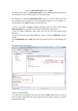


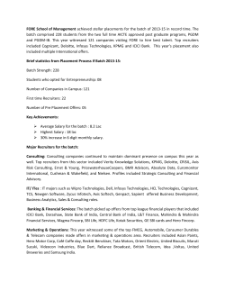
© Copyright 2026