
Merchandise Management
? Merchandise Management Subject: MERCHANDISE MANAGEMENT Credits: 4 SYLLABUS Product and Merchandise Management Introduction; Product Management; Brand Management in Retailing; Merchandise Management; Concentrating Factors Types of suppliers Types of Suppliers; Criteria for the Selection of Suppliers; Category Management; Merchandise Management Planning in Various Retail Segments Merchandise Management Assortment Merchandise Management Process; Forecasting Sales; Developing an Assortment Plan; Determine Variety and Assortment; Setting Inventory and Product Availability Levels, Indian Retail Scope Merchandise Planning System Staple Merchandise Management System; Fashion Merchandise Management System; Open-to Buy System, Allocating merchandise to stores Buying Merchandise Brand Alternatives; Buying National-Brand Merchandise; Buying Private-Label Merchandise, Strategic Relationship; Building Partnering Relationships Financial Merchandise Management Inventory Valuation: The Cost and Retail Methods of Accounting; Merchandise Forecasting and Budgeting; Unit Control System; Financial Inventory Control Pricing the merchandise in Retail Pricing Objective and Policies; Interaction between a Retailer’s Pricing ,Basic Markup Formulas; Markdown Management Suggested Readings: 1. Retail Management, by Michael Levy, Barton A Weitz, & Ajay Pandit, Publisher: The McGraw Hill publications. 2. Retail Management by Chetan Bajaj, Rajnish Tuli, & Nidhi V Srivastava, Publisher: Oxford University Press. 3. Retail Management: A strategic approach by Barry Berman and Joel R. Evans; Tenth Edition Published by Prentice-Hall, Inc. 4. Retailing Management by Michael Levy and Weitz Barton A, Publisher: John Wiley and Sons ----------------------------------------------------------------------------------------------------------------------- PRODUCT AND MERCHANDISE MANAGEMENT ----------------------------------------------------------------------------------------------------------------------- Structure 1.0 Introduction 1.1 Product Management 1.1.1 1.2 Aspects of Product Planning Brand Management in Retailing 1.2.1 Principles of Brand management 1.2.2 Types of Brands 1.3 Merchandise Management 1.4 Concentrating Factors ----------------------------------------------------------------------------------------------------------------------- 1.1 INTRODUCTION ----------------------------------------------------------------------------------------------------------------------Merchandising traces growth to the rise of organized retail in the world. Initially as the retailers operated one or two stores, the function of buying the merchandise, pricing it, etc was much simpler. In many cases the retailer himself did it. However, when retailers started adding stores and categories, the work load on the buyers increased significantly. Often buyers had little information or time and they ended up using approximations based on sales volumes to allocate merchadise between stores. This sometimes resulted in stores exchanging merchandise among them! In order to overcome this limitation, the function of a "PLANNER" came into being; the planner job was to act as a link between stores and the buyer. The de-linking of the functions allowed better interaction between the stores. Planners were able to devote more time to collect and study store level data, the buyers on the other hand were able to spend more time with the vendors Retail Merchandising is the process of developing, securing, pricing, supporting and communicating the retailer’s merchandise offering It means offering the right product at the right time at the right price with the right appeal!! 5 ----------------------------------------------------------------------------------------------------------------------- 1.1 PRODUCT MANAGEMENT ----------------------------------------------------------------------------------------------------------------------Product management is an organizational lifecycle function within a company dealing with the planning or marketing of a product or products at all stages of the product lifecycle. Product management (inbound focused) and product marketing (outbound focused) are different yet complementary efforts with the objective of maximizing sales revenues, market share, and profit margins. The role of product management spans many activities from strategic to tactical and varies based on the organizational structure of the company. Product management can be a function separate on its own or a member of marketing or engineering. While involved with the entire product lifecycle, product management's main focus is on driving new product development. According to the Product Development and Management Association (PDMA), superior and differentiated new products - ones that deliver unique benefits and superior value to the customer - is the number one driver of success and product profitability. 1.1.1 Aspects of product planning Depending on the company size and history, product management has a variety of functions and roles. Sometimes there is a product manager, and sometimes the role of product manager is held by others. Frequently there is Profit and Loss (P&L) responsibility as a key metric for evaluating product manager performance. In some companies, the product management function is the hub of many other activities around the product. In others, it is one of many things that need to happen to bring a product to market. Product planning • Defining new products • Gathering market requirements • Building product roadmaps, particularly Technology roadmaps • Product Life Cycle considerations • Product differentiation • more detail on Product planning Product marketing • Product positioning and outbound messaging • Promoting the product externally with press, customers, and partners • Bringing new products to market • Monitoring the competition • more detail on Product marketing 6 -----------------------------------------------------------------------------------------------------1.2 BRAND MANAGEMENT IN RETAILING ----------------------------------------------------------------------------------------------------------------------Brand management is the application of marketing techniques to a specific product, product line, or brand. It seeks to increase the product's perceived value to the customer and thereby increase brand franchise and brand equity. Marketers see a brand as an implied promise that the level of quality people have come to expect from a brand will continue with future purchases of the same product. This may increase sales by making a comparison with competing products more favorable. It may also enable the manufacturer to charge more for the product. The value of the brand is determined by the amount of profit it generates for the manufacturer. This can result from a combination of increased sales and increased price, and/or reduced COGS (cost of goods sold), and/or reduced or more efficient marketing investment. All of these enhancements may improve the profitability of a brand, and thus, "Brand Managers" often carry line-management accountability for a brand's P&L profitability, in contrast to marketing staff manager roles, which are allocated budgets from above, to manage and execute. In this regard, Brand Management is often viewed in organizations as a broader and more strategic role than Marketing alone. The annual list of the world’s most valuable brands, published by Inter- brand and Business Week, indicates that the market value of companies often consists largely of brand equity. Research by McKinsey & Company, a global consulting firm, in 2000 suggested that strong, well-leveraged brands produce higher returns to shareholders than weaker, narrower brands. Taken together, this means that brands seriously impact shareholder value, which ultimately makes branding a CEO responsibility. The discipline of brand management was started at Procter & Gamble PLC as a result of a famous memo by Neil H. McElroy. 1.2.1 Principles of Brand Management Here are some key principles of branding: 1. Brands are people. People make friends with people when they have things in common, want to spend time together, and find something special in the relationship. Brands make friends with people in exactly the same way. Brand management is about finding a group of people you can identify with, spending time together, & becoming committed to each other. The more time you spend with your customers the better. This is sometimes referred to as share of mind. 2. Branding is about the totality of a customer's experience. Your brand is about everything you do which impinges on the consciousness of the customer and, more importantly, it is about everything s/he thinks you do. Some experiences carry greater weight than others. Some experiences have been forgotten entirely consciously by your customer, but are nevertheless of paramount importance in the way s/he views you. Customers build brands piecemeal. They build a story about you based upon their experience. They see your products in certain shops. They heard one of your people on the radio. Somebody told them about an experience they had with you - actually, they got the name wrong. Your brand logo reminds them of daffodils. Your customer owns your brand - you do not. Your job is to behave as consistently as possible. 3. There are plenty of branding opportunities in any mass market place, so long as you do not try to copy the market leader. Brand marketing is about niche marketing. Different messages will appeal most to different groups of people. Be different. 7 4. 5. 6. 7. 8. 9. Brands are best communicated implicitly. Let the customer make the connection. You must try to facilitate that experience. The group of people on whom the brand is focused - the customers of the brand - need not necessarily pay you any money directly. Brands last forever, if managed correctly. The most exciting brands to have are icon brands that represent a certain moment in history. Icon brands grow rapidly, become outdated and decline, and can then bounce back on the next cycle of history. More traditional brands may have less ups and downs, but there will usually be fluctuations in their fortunes. Nevertheless, brands will tend to endure if invested in consistently. Consistency is one of the key underlying themes of branding. Brands win when they create a powerful experience that is totally compelling to the customer, and deliver it better than anyone else. The fewer the people you target with your brand, the more compelling is likely to be your claim in a highly competitive market. The more people you try to capture with your brand, the weaker may be your claim on any given customer, with one exception. In an environment where your customers do not have a relationship with any brands in particular, they will probably be drawn to those they recognise the best. Brands are therefore a bit like light beams. The more concentrated the beam, the more cutting power it will have (as in a laser beam); however, even a diffuse beam, like sunlight, will shed more light and heat than will darkness. As brands are people, they can be analysed like people. There are two psychological theories that are especially relevant to the analysis of brands: Personal Construct Theory - this theory argues that individuals develop theories (constructs) about how the world works, what values are to be espoused, and how personal success is achieved. These constructs are specific to the individual and bi-polar - they exist along a scale between two points defined by the individual. While one person may contrast hard vs. soft, another may contrast hard vs. squelchy, or hard vs. weak. For some, a construct may be close to the centre of how they assess other people, for others it may be peripheral, or even irrelevant. People generally prefer to discuss peripheral constructs with strangers & acquaintances as they are easily abandoned or adapted. The core constructs, which they hold closest to their hearts, are rarely mentioned. However, by the application of a technique called laddering, a good interviewer can begin to discover individuals' core constructs by starting with their peripheral ones. Attribution theory - this theory argues that people ascribe characters to the people they meet based on a very few clues around which they spin elaborate stories. So from a gesture, or a turn of phrase, or an intonation of voice, they quickly come to a conclusion as to the sort of person they are dealing with (often within 20 seconds of meeting the person, in fact). These judgments are made not only of people, but also of animals (anthropomorphism), and even of inanimate objects (what human characteristics do you ascribe to your computer when it crashes?). Brands, which function as fictional people, are also ascribed human characteristics. Brands can therefore be analysed along two key dimensions: • The level of intimacy they have with their customers • Their level of stature in the world Elements that will drive these dimensions are: • The central organising thought of the brand • The personality of the brand 8 The values the brand espouses The tastes/dress of the brand, including how it speaks The emotional benefits the brand satisfies The hard benefits the brand delivers to the customer There is evidence that measures of stature in particular (such as Total Research's Relative Perceived Quality) have strong correlations with sales, the ability to charge a premium for your products and services, and even stock price. • • • • Imagine achieving so much more for so much less. We can help you in two ways - we have a mass of smart strategic brand marketing tools, processes and workshop techniques for you to use, and a mass of smart brand marketing agencies as members across the world with niche knowledge and experience to support you thereafter. A good brand name should: • be protected (or at least protectable) under trademark law • be easy to pronounce • be easy to remember • be easy to recognize • be easy to translate into all languages in the markets where the brand will be used • attract attention • suggest product benefits (e.g.: Easy-Off) or suggest usage (note the tradeoff with strong trademark protection) • suggest the company or product image • Distinguish the product's positioning relative to the competition. • be attractive • stand out among a group of other brands 1.2.2 Types of brands A number of different types of brands are recognized. A "premium brand" typically costs more than other products in the same category. An "economy brand" is a brand targeted to a high price elasticity market segment. A "fighting brand" is a brand created specifically to counter a competitive threat. When a company's name is used as a product brand name, this is referred to as corporate branding. When one brand name is used for several related products, this is referred to as family branding. When all a company's products are given different brand names, this is referred to as individual branding. When a company uses the brand equity associated with an existing brand name to introduce a new product or product line, this is referred to as "brand leveraging." When large retailers buy products in bulk from manufacturers and put their own brand name on them, this is called private branding, store brand, white labeling, private label or own brand (UK). Private brands can be differentiated from "manufacturers' brands" (also referred to as "national brands"). When two or more brands work together to market their products, this is referred to as "cobranding". When a company sells the rights to use a brand name to another company for use on a non-competing product or in another geographical area, this is referred to as "brand licensing." An "employment brand" is created when a company wants to build awareness with potential candidates. In many cases, such as Google, this brand is an integrated extension of their customer. 9 ----------------------------------------------------------------------------------------------------------------------- 1.3 MERCHANDISE MANAGEMENT ----------------------------------------------------------------------------------------------------------------------Steps in the Retail Merchandising Process 1. Develop the merchandise mix and establish the merchandise budget. 2. Build the logistic system for procuring the merchandise mix. 3. Price the merchandise offering. 4. Organize the customer support service and manage the personal selling effort. 5. Create the retailer’s advertising, sales incentive and publicity programs. Retail Merchandising is the process of developing, securing, pricing, supporting and communicating the retailer’s merchandise offering. It means offering the right product at the right time at the right price with the right appeal!! Retail merchandising requires management of the merchandise mix including: 1. Planning Merchandise Variety 2. Controlling Merchandise Variety 3. Planning Merchandise Assortment/Support 4. Controlling Merchandise Assortment/Support 5. Merchandise Mix Strategies Developing the merchandise mix allows the retailer to segment the market and appeal to a select group of consumers!! Retail merchandising requires management of the merchandise budget including: 1. Planning And Controlling Retail Sales 2. Planning And Controlling Inventory Levels 3. Planning And Controlling Retail Reductions 4. Planning And Controlling Purchases 5. Planning And Controlling Profit Margins The Components of the Merchandise Mix ¾ Merchandise Variety (# of product lines) ¾ Merchandise Assortment (# of product items) ¾ Merchandise Support (#of product units) ----------------------------------------------------------------------------------------------------------------------- 1.4 CONCENTRATING FACTORS ----------------------------------------------------------------------------------------------------------------------There are many applications that call for the determination of the points at which a function changes values in a discontinuous fashion and that require knowledge of the change in the function's value at such points. In this paper we present some simple examples of concentration 10 factors. Concentration factors take the Fourier coercions of a function and return a function that tends to zero at points of continuity of the original function and that tends to the height of the jumps at the location of the jumps. In the analysis of concentration factors, we make use of many elementary results from analysis and many properties of Fourier series. The material here except for the last section can be presented to anyone with a reasonable knowledge of Fourier series and a decent understanding of the properties of innate series. In the ¯operational section, we consider the eject that noisy data has on the results of the schemes we present. Concentration factors, Fourier series, harmonic series, noise AMS subject classifications. 1. Introduction. Edge detection and the detection of discontinuities are very important in many fields. In image processing, for example, one often need to determine the boundaries of the items of which a picture is composed. (For more information about edge detection in image processing. We consider the problem of detecting the edges present in a function when given the Fourier coercions of the function. There are numerical methods that estimate the Fourier coercions of a function of interest rather than directly estimating the solution. The spectral viscosity method, a numerical method used to solve nonlinear partial differential equations (PDEs), is an example of such a method. The method approximates the Fourier coercions of the solution of a PDE. The Fourier coercions are then used to calculate an approximation to the solution. The accurate reconstruction of the solution requires that the position of the discontinuities of the solution be known. In this paper we discuss techniques for using a function's Fourier coercions to determine the location and size of the jump discontinuities of the function. At first glance the spectral representation of the signal the Fourier series or transform associated with the signal does not seem to be the ideal place to look for information about discontinuities in the signal. When a signal is discontinuous the convergence of the Fourier series or transform associated with the signal is not uniform; in such cases the Gibbs phenomenon appears and truncating the series after any nite number of terms always leads to O oscillations in the reconstructed signal. Considering the question again, however, one realizes that if a discontinuity is characterized by a \phenomenon," then the existence of the discontinuity is indeed encoded in the coercions. The question becomes how to electively “decode" the discontinuity. One does not do this by directly summing the series one uses the spectral representation in a somewhat deferent way to concentrate" the function about the discontinuity. In what follows, we explain how this is done. We restrict ourselves to periodic (or compactly supported) functions and only consider Fourier Much of the information in this article is well known [3, 4]. The use of the Euler- Mascheroni constant to improve the performance of the concentration factor in x4 and the noise analysis in x6 are new to the best of our knowledge. In the next section we give some of the background necessary for our study. In the following sections we present the classical method of finding the discontinuities, we explain its shortcomings, we present a better method and analyze its properties, and we explore the behavior of the methods in the presence of noise. 11 ------------------------------------------------------------------------------------------------------------ TYPES OF SUPPLIERS ------------------------------------------------------------------------------------------------------------ Structure 2.0 Types of suppliers 2.1 Criteria for the Selection of Suppliers 2.2 Category Management 2.3 Merchandise Management Planning in Various Retail Segments -------------------------------------------------------------------------------------------2.0 TYPES OF SUPPLIERS -----------------------------------------------------------------------------------------------------------Types of suppliers include: • Manufacturer, uses tools and labor to make things for sale. • Processor (manufacturing), converts a product from one form to another. • Packager (manufacturing), encloses products for distribution, storage, sale, and use. • Distributor (business), the middleman between the manufacturer and retailer. • Wholesaler, sells goods or merchandise to retailers. • Dealership, local franchised distribution. • Drug dealer, supplies illegal drugs. • Merchant, a professional dealing with trade . Manufacturing is the use of machines, tools and labor to make things for use or sale. The term may refer to a range of human activity, from handicraft to high tech, but is most commonly applied to industrial production, in which raw materials are transformed into finished goods on a large scale. Such finished goods may be used for manufacturing other, more complex products, such as household appliances or automobiles, or sold to wholesalers, who in turn sell them to retailers, who then sell them to end users - the "consumers”. Manufacturing takes turns under all types of economic systems. In a free market economy, manufacturing is usually directed toward the mass production of products for sale to consumers at a profit. In a collectivist economy, manufacturing is more frequently directed by the state to supply a centrally planned economy. In free market economies, manufacturing occurs under some degree of government regulation. Modern manufacturing includes all intermediate processes required for the production and integration of a product's components. Some industries, such as semiconductor and steel manufacturers use the term fabrication instead. 12 The manufacturing sector is closely connected with engineering and industrial design. Examples of major manufacturers in the United States include General Motors Corporation, Ford Motor Company, Chrysler, Boeing, Gates Rubber Company and Pfizer. Examples in Europe include Airbus, Daimler, BMW, Fiat, and Michelin Tyre. Processing typically describes the act of taking something through an established and usually routine set of procedures to convert it from one form to another, as a manufacturing procedure, such as processing milk into cheese. Processing can also refer to administrative procedure such as processing paperwork to grant a mortgage loan. Processing can refer to: • Data processing • Food processing • Geometry processing • Information processing • Process industries • Processing technique of altering the properties of crude drugs by such means as roasting, honey frying, wine frying, earth frying, vinegar frying, calcining, or other means • Processing (programming language) • Signal processing • Word processing Packaging is the science, art and technology of enclosing or protecting products for distribution, storage, sale, and use. Packaging also refers to the process of design, evaluation, and production of packages. Package labeling (BrE) or labeling (AmE) is any written, electronic, or graphic communications on the packaging or on a separate but associated label. Packaging can be described as a coordinated system of preparing goods for transport, warehousing, logistics, sale, and end use. Packaging contains, protects, preserves, transports, informs, and sells. It is fully integrated into government, business, institutional, industry, and personal use. Packaging is the science, art and technology of enclosing or protecting products for distribution, storage, sale, and use. Packaging also refers to the process of design, evaluation, and production of packages. Package labeling (BrE) or labeling (AmE) is any written, electronic, or graphic communications on the packaging or on a separate but associated label. Packaging can be described as a coordinated system of preparing goods for transport, warehousing, logistics, sale, and end use. Packaging contains, protects, preserves, transports, informs, and sells. It is fully integrated into government, business, institutional, industry, and personal use. Distribution (or place) is one of the four elements of marketing mix. An organization or set of organizations (go-betweens) involved in the process of making a product or service available for use or consumption by a consumer or business user. The other three parts of the marketing mix are product, pricing, and promotion. 13 Wholesaling, historically called jobbing, is the sale of goods or merchandise to retailers, to industrial, commercial, institutional, or other professional business users, or to other wholesalers and related subordinated services. According to the United Nations Statistics Division, "wholesale" is the resale (sale without transformation) of new and used goods to retailers, to industrial, commercial, institutional or professional users, or to other wholesalers, or involves acting as an agent or broker in buying merchandise for, or selling merchandise to, such persons or companies. Wholesalers frequently physically assemble sort and grade goods in large lots, break bulk, repack and redistribute in smaller lots. While wholesalers of most products usually operate from independent premises, wholesale marketing for foodstuffs can take place at specific wholesale markets where all traders are congregated. Merchants function as professionals who deal with trade, dealing in commodities that they do not produce themselves, in order to produce profit. Merchants can be of two types: 1. A wholesale merchant operates in the chain between producer and retail merchant. Some wholesale merchants only organize the movement of goods rather than move the goods themselves. 2. A retail merchant or retailer, sells commodities to consumers (including businesses). A shop owner is a retail merchant. A merchant class characterizes many pre-modern societies. Its status can range from high (even achieving titles like that of merchant prince or nabob) to low, such as in Chinese culture, due to the soiling capabilities of profiting from "mere" trade, rather than from the labor of others reflected in agricultural produce, craftsmanship, and tribute. ------------------------------------------------------------------------------------------------------------ 2.1 CRITERIA FOR THE SELECTION OF SUPPLIERS -----------------------------------------------------------------------------------------------------------Supplier Selection Strategies and Criteria Supplier selection criteria for a particular product or service category should be defined by a “cross-functional” team of representatives from different sectors of your organization. In a manufacturing company, for example, members of the team typically would include representatives from purchasing, quality, engineering and production. Team members should include personnel with technical/applications knowledge of the product or service to be purchased, as well as members of the department that uses the purchased item. I. Common supplier selection criteria: • • Previous experience and past performance with the product/service to be purchased. Relative level of sophistication of the quality system, including meeting regulatory requirements or mandated quality system registration (for example, ISO 9001, QS-9000). 14 • • • • • • Ability to meet current and potential capacity requirements, and do so on the desired delivery schedule. Financial stability. Technical support availability and willingness to participate as a partner in developing and optimizing design and a long-term relationship. Total cost of dealing with the supplier (including material cost, communications methods, inventory requirements and incoming verification required). The supplier's track record for business-performance improvement. Total cost assessment. Methods for determining how well a potential supplier fits the criteria: • Obtaining a Dun & Bradstreet or other publicly available financial report. • Requesting a formal quote, which includes providing the supplier with specifications and other requirements (for example, testing). • Visits to the supplier by management and/or the selection team. • Confirmation of quality system status either by on-site assessment, a written survey or request for a certificate of quality system registration. • Discussions with other customers served by the supplier. • Review of databases or industry sources for the product line and supplier. • Evaluation (SUCH AS prototyping, lab tests, OR validation testing) of samples obtained from the supplier. Selection of the best possible set of suppliers has a significant impact on the overall profitability and success of any business. For this reason, it is usually necessary to optimize all business processes and to make use of cost-effective alternatives for additional savings. This paper proposes a new efficient context-aware supplier selection model that takes into account possible changes of the environment while significantly reducing selection costs. The proposed model is based on data clustering techniques while inspiring certain principles of online algorithms for an optimally selection of suppliers. Unlike common selection models which re-run the selection algorithm from the scratch-line for any decision-making sub-period on the whole environment, our model considers the changes only and superimposes it to the previously defined best set of suppliers to obtain a new best set of suppliers. Therefore, any re-computation of unchanged elements of the environment is avoided and selection costs are consequently reduced significantly. A numerical evaluation confirms applicability of this model and proves that it is a more optimal solution compared with common static selection models in this field. N modern business, a key tool for success is supplier selection mechanism as it has a significant bearing on the performance and overall-profitability of the business. Qualified suppliers, at right quantities and when required, make the related business fruitful and promising. Therefore, upgrading such mechanism is a major concern in the commercialrelated researches and forms the basis of an extensive research from which this paper has been extracted. As is illustrated in figure 2.1, supplier selection process is usually consists of four steps. The first step, Problem Definition Step, concerns decision makings which should determine the strategy of purchases e.g. the duration of new selection. Second 15 stage of this process is called Decision Criteria Formulation. Depending on the purchasing situation, the multi-criteria nature of selecting the right suppliers may force some complexity to this decision. The best set of selection criteria is carefully determined in this phase. Pre-Selection of Potential Suppliers, the third step, the set of alternatives is refined with respect to the ability of satisfying a minimal threshold. Final Selection is the last phase in the supplier selection process. At this stage, ultimate suppliers are identified and orders are allocated among them while considering the system’s constraints and taking into account a multitude of criteria. Fig 2.1 General Supplier Selection Flowchart There are several variations of decision models and techniques which are proposed to accomplish this task. A general classification of existing techniques regarding the supplier selection process suggested in is as follows: o Single objective techniques: o Linear Programming Method o Mixed-integer Programming Method 16 o Non-linear Programming Method o Dynamic Programming o Stochastic Programming o Decision Theory o Multiple objective techniques: o Multi-objective Programming Method o Goal Programming Method o Other Methods such as Neural Networks. However, a fresh computing procedure, called ubiquitous/pervasive computing, that employs new means of automation and computation without explicit involvement of human has been emerged recently. Due to its potentials in establishing communication between human (or other objects) with computing systems, as it runs in the background of everyday life of people and tries not to be sensed by human, it is nicknamed as the calmest technology . Currently, the most focused issue in ubiquitous/pervasive computing field is context-aware computing. A context-aware system is able to adapt its operations to a given context, without explicit user intervention and thus aims at increasing usability and effectiveness by taking environmental context into account. As proposed by Dey and Abowd, “context” may be defined as “any information that can be used to characterize the situation of entities (i.e. a person, place or object) that are considered relevant to the interaction between a user and an application, including the user and the application themselves”. According to this definition, three distinct entities are identified concerning context, namely Places, People and Things. Each entity is characterized by certain attributes such as identity, location, status and time. Regarding the pervasive computing concepts, our new idea in this work is to apply the basis of context-awareness in the supplier selection process so that it can run in the background of business and adapt the best set of suppliers to the changes of the environment. In developing a context-aware supplier selection model, the environment may be identified as a set of possible supply candidates which may be changed in course of time. For example, suppliers frequently change their products’ price in response to the governing political/social/financial conditions; new suppliers may appear and certain supplier may even lunch new trade strategies for boosting their business. Context, therefore, should also reflect these evolving-candidates’ influences. To make the supplier selection process adaptable to the changes of the environment, one may suggest a re-run of the selection model every time a minor change takes place. However, most of current selection models are static in their nature and consider just a single snapshot of the environment at a time without considering changes’ effects to the past and future states (i.e. they don’t consider the changes in suppliers’ status in the course of time). For this reason, in static selection 17 models, a combination of changed and unchanged elements (i.e. candidate suppliers) are to be re-considered as a new set-up to make the selection process fair. This imposes additional computational cost and time to the business and, therefore, may inversely affect its overall profitability. To develop a cost-efficient context-aware supplier selection model, online algorithms concepts and data clustering techniques has been used in this work. The proposed selection model is capable for considering all changes in the environment at each decision making step while making use of the solutions found in the past sub-periods. Therefore, the proposed model can find the new optimum set of suppliers while minimizing the overall cost of performing this process. Within the remaining parts of this paper followings are covered: in section 2 a brief review of online algorithms and data clustering techniques are presented. The so-called context-aware supplier selection model for time-sensitive supplies is discussed in the third section. The result of evaluating the proposed selection model is demonstrated in section 4 and finally sections 5 presents some concluding remarks. II. Background Online algorithms In one of decision-making process that is commonly known as online decision algorithms, a sequence of decisions can be made with minimal knowledge of future events. In other words, an online algorithm does not rely on immediate access to the entire information concerning a given problem. Instead, the problem is revealed to the algorithm incrementally, and in response to each incomplete portion of the input, the algorithm must take an irreversible action with no access to the future input. Since in our supplier selection problem, changes in the candidates’ environment usually occur incrementally, the online algorithms may be regarded as a powerful means for decision making at first glance. However, applicability of the available online algorithms with such specific usage is not a straight forward task and there exist certain constraints in their usage in this field. For example, a pioneer work on this subject considers a randomized “follow the expected leader” algorithm whiles the work in utilizes a deterministic algorithm based on the expected gradient ascent. Another class of thoughts in this field is based on Aggregating Algorithm (AA), for solving online decision problems optimally. One common feature in all versions of online algorithms, however, is their lengthy computational requirements due to their complicated mathematical basis which make them expensive tools for commercial applications. In other words, as our immediate goal in this work is to lunch a new context-aware supplier selection model while minimizing the computational cost, none of existing online algorithms seems to be capable of fulfilling such requirement and decreasing the selection costs. Therefore, we only inspired from the nature of these algorithms in developing our online supplier selection model. B. Data Clustering In all aspects of human life, one of the most important means in analyzing phenomena and objects is classifying them into categories or clusters in order to extract their describing features and, also, comparing them with other objects or phenomena on the basis of their similarities and dissimilarities . Theoretically, classification systems are either supervised or unsupervised, depending on whether they assign new inputs to one of a finite number of discrete supervised classes or unsupervised categories, respectively. In supervised classification, the mapping from a 18 set of input data vectors (where d is the input space dimensionality), to a finite set of discrete class labels, is modeled in terms of some mathematical function . In unsupervised classification, called clustering or exploratory data analysis, no labeled data are available. The goal of clustering is to separate a finite unlabeled data set into a finite and discrete set of “natural,” hidden data structures, rather than provide an accurate characterization of unobserved samples generated from the same probability distribution . Clustering techniques are useful in several exploratory pattern-analysis, grouping, decision-making, and machine learning applications. Some times there exist little prior information (e.g., statistical models) and decision-maker also has to make as few assumptions about the data as possible. In these situations clustering methodology is particularly appropriate for exploring interrelationships between data points in order to make an assessment of their structure. Selecting one of different clustering techniques depends on the nature of the problem to be solved. Theoretically, these techniques may be classified as hierarchical and nonhierarchical clustering algorithms. Hierarchical techniques, such as Growing Hierarchy Self Organizing Map (GHSOM) clustering, produce a nested set of partitions and are usually employed in discovering natural structure of some phenomena. While, nonhierarchical clustering methods only partition data into a pre-specified set of clusters such as Self Organizing Map (SOM) method. In addition to the above mentioned major classes, other clustering alternatives such as fuzzy clustering, nearest neighbor clustering and evolutionary algorithms for clustering have been developed. Evolutionary approaches, motivated by natural evolution, make use of evolutionary operators and a number of solutions to obtain the globally optimal partition of the data. In other words, unlike other clustering methods which work with static data sets - data that neither move, nor disappear nor emerge - evolutionary clustering algorithms consider dynamic data set and try to obtain the globally optimal cluster set of data. Some researchers have considered evolution of clusters of dynamic data sets. The most recent effort proposes a novel method for online clustering of the dynamic data set, based on state space model where the measurement equation is represented by a Gaussian mixture with unknown number of components where the state equation is not explicit. They solve this problem by deriving a SEM algorithm which updates the current clustering from a window of snapshots of the dynamics data set; Evolutionary clustering technique offers an attractive tool in developing a context-aware supplier selection model due to its dynamic nature. However, its theoretical complexity as well as its high computational cost, prohibits its applicability in our problem. For this reason, static clustering algorithms seem to be more appropriate to our work. From several alternatives of static clustering algorithms we have chosen GHSOM method. As the hierarchy of clusters is not important in supplier selection problem, we have used it just in layer one. On the ground of supplier selection, every single data is regarded as a vector composed of some components. These components are the criteria chosen for selection process. For every supplier a value is to be assigned to these selection criteria by means of which the vector is capable of describing a particular supplier. In clustering a given set of candidates, it is preferable to life restrictions on the number of clusters to a predefined value as the number of clusters may vary because of emergence and elimination of candidates. For this reason, GHSOM is a promising clustering algorithm that eliminates the need for predefining the number of 19 clusters. Every added/removed data can change the quality of the cluster that it belongs to. Clusters’ quality, therefore, should be monitored constantly. By predefining a quality threshold, when the set threshold is reached, a bad cluster has to be split into new smaller clusters with qualities below that threshold. We consider a bad cluster as a new map that requires a re-run of GHSOM. To measure quality of a cluster, we have adapted the sum of Weighted Euclidean Distance of data from the reference vector of their immediate cluster that has been suggested by GHSOM itself. III. The Proposed Model This model represents the overall framework of our approach by adapting the general supplier selection framework. A. Problem Definition Similar to other selection models, our first step is Problem Definition step (see Fig.2.1) in which the overall planning period for selecting appropriate suppliers is determined. This is a planning-level decision, and may be as long as one year or may be as short as a quarter of a year and is called “total selection period”. Then the so-called “selection subperiods” are to be defined as fractions of total selection period depending on the strategy of the firm. B. Decision Criteria Formulation The second step, the Decision Criteria Formulation step, consists of two categories of criteria to be considered. The first category concern is the supply profits and is formed by those criteria having direct impact on the profitability potential of selected suppliers. The second category consists of those criteria handling the supply risk and includes variances of influential supply profit criteria, such as variance of price or variance of quality. The greater a variance, the more risky would be selecting that candidate. We have chosen quality, quantity, price, delivery-cost, delivery-capacity, delivery-lead-time as the supply profit criteria. The quality of supplied materials is defined as the number of defected items in a lot, and the quantity is the capability of the supplier to meet orders. The price criterion is the offered cost-price per unit of supplied items. Delivery criterion is handled by the flow networking techniques. Regarding the nature of flow networks, the unit cost of delivering the supplied material to the producer, delivery-cost, and the capacity of the flow (road) between supplier and producer, delivery-capacity, is covered. To consider the lead-time factor, i.e. the required time for delivery of goods (deliverylead-time), another selection criterion is also included. In our model, no allowance has been given to the supply risk criterion. However, to handle the supply risk, we employed a new strategy which is more reliable and runs in the context of selection process. Unlike a proposed approach in that handles the supply risk by means of the value of some supply profit criteria at variance with its value from immediate previous sub-period, our risk management technique considers a history of criteria from T0 (first sub period) to present (Tt-1) in order to monitor the long term performance of all suppliers. This technique enables us to find out the degree of trustability of suppliers in the future. The technique is based on a statistical regression 20 Fig 2.2 The Selection Flowchart function and makes certain decisions in accordance with its forecasts for the subsequent sub-period. C. Selection Two final steps of general supplier selection framework are combined to form the Selection step in our model. This is the most important development in the proposed framework and consists of some sub-phases as shown in Fig. 2.2 21 1) Start-up This phase is to be run at T0 only. At the first sub-period, we assume having no preknowledge about the environment. Therefore, one of common static supplier selection models must be employed. The model described in seems to fit better than other methods as it clusters the candidates by means of three supply profit criteria (quality, quantity and price). This static selection model at T0 provides a set of the best suppliers. 2) Applying changes At the beginning of the subsequent sub-period (Tt-1), we have a changed set of candidates. Any potential supplying offer may undergo changes (e.g. changes in price and/or quality), some supplier may seize activity, and fresh candidate may appear at this time. Therefore, it is essential to consider theses changes and accommodate them within new appropriate clusters. As pointed out in changing data may lead to changes in the quality of clusters. Clusters with a quality below the specified threshold should be split (Fig.2.3). By the end of this phase a new state of environment forms. Fig 2.3 Splitting a Bad Quality Cluster 3) Cluster Evaluation Having a changed environment of candidates, candidates should then be evaluated and scored subsequently. To safeguard the ultimate goal of reducing computational cost, we perform the evaluation process at a concise cluster level. As mentioned before, a group of data that forms a cluster has commonly a reference vector representing that particular cluster. These indices in our model act as abstractions of data and may be evaluated instead of actual clusters. The evaluation process is based on two advanced criteria belonging to the supply risk category. The first criterion concerns historical performance analysis of a given cluster in which a sequence of the cluster performance in previous sub-periods are plotted by means of statistical regression methods in order to enable forecasting cluster’s performance in the subsequent sub-period. 4) Supplier Evaluation and Order Allocation At this step ultimate suppliers are selected on the basis of assigned scores and orders allocations are made amongst them. To perform this task, candidates in the first best clusters are to be evaluated by means of delivery-capacity, delivery cost and deliverylead-time criteria. This is noteworthy that separating the delivery-related criteria and 22 supply profit criteria allows similar candidate to change there geographical location without any impact on their evaluation. We call this type of candidate as “mobile suppliers”. IV. Evaluation To evaluate the proposed context-aware supplier selection model, a set of 100 supplying candidates for a given industry were considered. The “total selection period” was assumed to be in order of six months and each “selection sub-period” lasts after exactly one month leading to six sub-periods: T0, T1… T5. Then a mixed-integer programming model – that is believed to be a similar approach was considered as a stand comparison for assessing effectiveness of the proposed model from three different points of view including number of selected suppliers, total supply costs and the computational costs. The number of selected suppliers is important as a greater number of selected suppliers causes more difficulties in managing them and imposes more additional costs to the business. As shown in Fig.2.4, our context-aware supplier selection model is capable to meet the orders with fewer numbers of suppliers. Fig 2.4 Number of Selected Suppliers per Period The total supply cost that should be paid by a business is a function of offered prices, delivery costs and switching costs. In mathematical terms it may be written as: Total supply cost = (price × allocated order) + (delivery costs × allocated order) + switching costs. Selecting the best possible suppliers is commonly regarded as a crucial issue due to its bearings on the total profitability and success of any business. Optimization of this 23 business-process and reducing its potential inflating costs, therefore, is an important field of studies in the modern commerce. The emergence of new computing procedures such as pervasive computing, introduces new means for performing processes of a business more efficiently. In this area, context-aware computing develops systems which are able to adapt themselves to changes of the environment without explicit intervention of human. Hence, by applying the concept of context-awareness in the supplier selection process, it may be possible to significantly improve profitability of a business. To formulate a context-aware supplier selection model on the basis of the current static selection models may force a business to re-run the selection processes all over again on the whole set of candidates to find the new best set of suppliers regardless of the severity of the environment changes, which is usually minor. This increases computational cost that may be avoided by considering changes only and making use of the previously selected set of suppliers for subsequent sub-period. ------------------------------------------------------------------------------------------------------------ 2.2 CATEGORY MANAGEMENT -----------------------------------------------------------------------------------------------------------Category Management is a retailing concept in which the total range of products sold by a retailer is broken down into discrete groups of similar or related products; these groups are known as product categories. Examples of grocery categories may be: tinned fish, washing detergent, toothpastes, etc. Each category is then run like a "mini business" (Business Unit) in its own right, with its own set of turnover and/or profitability targets and strategies. An important facet of Category Management is the shift in relationship between retailer and supplier : instead of the traditional adversarial relationship, the relationship moves to one of collaboration, exchange of information and data and joint business. The focus of all negotiations is centered on the effects of the turnover of the total category, not just the sales on the individual products therein. Suppliers are expected, indeed in many cases, mandated to only suggest new product introductions, a new Planogram or promotional activity if it is expected to have a beneficial effect on the turnover or profit of the total category and be beneficial to the shoppers of that category. The concept was initiated, and is still most commonly found in Grocery (Mass merchandising) retailing, but now also found in other retail sectors such as DIY, Cash and Carry, Pharmacy/Drugstore and even Book retailing. Definition of Category Management Category Management lacks a single definition thus leading to some ambiguity even among industry professionals as to its exact function. Three comparative mainstream definitions are as follows: Category Management is a process that involves managing product categories as business units and customizing them [on a store by store basis] to satisfy customer needs. 24 The strategic management of product groups through trade partnerships which aim to maximize sales and profit by satisfying consumer and shopper needs (Institute of Grocery Distribution) Marketing strategy in which a full line of products (instead of the individual products or brands) is managed as a strategic business unit (SBU). (Business Dictionary) The Nielsen definition, published in 1992, was a little ahead of its time in that customising product offerings on a store by store basis is logistically difficult and is now not considered a necessary part of Category Management; it is a concept now referred to as micromarketing. Nevertheless, most grocery retailers will segment stores at least by size, and select product assortments accordingly. Wal Mart's Store of the Community, implemented in North America is one of the few examples of where product offerings are tailored right down to the specific store. One key reason for the introduction of Category Management was the retailers' desire for suppliers to add value to their (ie the retailer's) business rather than just the supplier's own. For example, in a category containing brands A and B, the situation could arise such that every time brand A promoted its products, the sales of brand B would go down by the amount that brand A would increase, resulting in no net gain for the retailer. The introduction of Category Management imposed the condition that all actions undertaken, such new promotions, new products, re-vamped plano-gram, introduction of Point of Sale advertising etc. were beneficial to the retailer and the shopper in the store. A second reason was the realisation that only a finite amount of profit could be milked from price negotiations and that there was more profit to be made in increasing the total level of sales. A third reason was that the collaboration with the supplier meant that supplier's expertise about the market could be drawn upon, and also that a considerable amount of workload in developing the category could be delegated to the supplier. The Nielsen definition of a category, used as the basic definition across the industry is that the products should meet a similar consumer need, or that the products should be inter-related or substitutable. The Nielsen definition also includes a proviso that products placed together in the same category should be logistically manageable in store (for example there may be issues in having room-temperature and chilled products together in the same category even though the initial two conditions are met). However, this definition does not explain how the process often works in practical retailing situations. For example, electric toothbrushes are often placed in a separate "electricals" category with hair driers and not with manual toothbrushes, even though the Nielsen definition may suggest otherwise. Sometimes demographic considerations overrule, so luxury chrome toilet brushes could be found in a luxury-bathroom-fittings category, totally separate from the white plastic toilet brushes placed in the household brushes category. Depending on the size and internal structure of the retailer, different definitions may exist: whereas one retailer may have a tinned tomatoes category, another may consider it just a small sub-segment of a larger tinned vegetables category. 25 The Category Management 8 Step Process Fig 2.5 The industry standard model for Category Management is the 8-step process, or 8-step cycle developed by the Partnering Group. The eight steps are shown in the diagram on the right; they are: 1. Define the Category (i.e. what products are included/ excluded). 2. Define the role of the category within the retailer. 3. Assess the current performance. 4. Set objectives and targets for the category. 5. Devise an overall Strategy. 6. Devise specific tactics. 7. Implementation. 8. The eighth step is one of review which takes us back to step 1. 26 The 8-step process, whilst being very comprehensive and thorough has been criticized for being rather too unwieldy and time-consuming in today's fast-moving sales environment; in one survey only 9% of supplier companies stated they used the full 8-step process. The current industry trend is for supplier companies to use the standard process as a basis to develop their own more streamlined processes, tailored to their own particular products. Market Research Company Nielsen has a similar process based on only 5 steps: Reviewing the Category, Targeting consumers, Planning merchandising, Implementing strategy, evaluating results. Category Captains It is commonplace for one particular supplier into a category to be nominated by the retailer as a Category Captain. The Category Captain will be expected to have the closest and most regular contact with the retailer and will also be expected to invest time, effort, and often financial investment into the strategic development of the category within the retailer. In return for this, the supplier will gain a more influential voice with the retailer but must be careful never to abuse this or fall foul of any antitrust laws. The Category Captain is often - but not always! - The supplier with the largest turnover in the category. Traditionally the job of Category Captain is given to a brand supplier but in recent times the role has also gone to particularly switched-on Private label suppliers. In order to do the job effectively, the supplier may be granted access to a greater wealth of data-sharing, eg more access to an internal sales database such as Walmart's Retail Link. ------------------------------------------------------------------------------------------------------------ 2.3 MERCHANDISE MANAGEMENT PLANNING IN VARIOUS RETAIL SEGMENTS WITH EMERGING TECHNOLOGIES ERP -----------------------------------------------------------------------------------------------------------Enterprise Resource Planning systems or the ERP systems refer to the software packages that integrate all the data and the related processes of an organization into a unified Information System (IS). An ERP system uses a central database that holds all the data relating to the various system modules. In order to achieve a seamless integration, an ERP system uses multiple hardware and software components. ERP packages are heavily used by larger retail chains. Designed to facilitate the administration and optimization of internal business processes across an enterprise, ERP packages have become the competitive tool for most large retail organizations. An ERP software uses a single database that allows the different departments to communicate with each other through information sharing. ERP systems comprise function-specific components that are designed to interact with the other modules such as the Order Entry, Accounts Payable, Accounts Receivable, Purchasing, Distribution etc. 27 Fig 2.6 Components of an ERP system Components of an ERP system ERP systems comprise of different modules such as order entry, purchase, sales, finances, inventory management, DRP (Distribution Resource Planning) and human resources. The components are designed to work effortlessly with the rest of the system and provide a consistent user interface throughout the system. ERP software packages have an enterprise wide reach that offers cross-functional capabilities to the organization. The different functional departments involved in the operations or inventory processes are integrated into a single system. An ERP package takes care of the various business processes such as order entry, logistics and warehousing. It also caters to the different business functions such as accounting, marketing, strategic management and the human resource management. In the current business environment, the retail industry faces two major challenges that threaten its profitability and the long-term survival prospects. The twin challenges are: 1 Market competition – To beat the competition, retailers have to understand consumer demand at the point of interaction and respond to the various inputs in real time across the enterprise. This calls for a proactive approach on the part of the retail organization to sense the specific requirements of the consumer before other competitors and respond to them in real-time ensuring customer satisfaction in the process. Moreover, margins in the retail business generally are very low and that removes any scope for waste or inefficiencies in the business processes. Efficiency is critical to survive in the retail industry. A proactive approach on the part of the retail organization requires an enterprise wide monitoring and control of the various 28 2 3 business processes that may ultimately lead to the desired efficiencies and long-term customer satisfaction and profitability. Regulatory pressures – In order to meet the regulatory standards, the retailers require an enterprise wide process visibility, data access and near-instant performance reporting. However, the need for flexibility, process efficiency, reliable information, and responsiveness is very hard to achieve given the existing portfolio of legacy, home grown and packaged software applications used by a majority of the retail organizations. Therefore, a retail business would benefit immensely from an integrated IS infrastructure which continuously monitors and dispatches the necessary information of the flow of goods all the way from supplier to the cash register and then back to accounting as well as other functions of the retail organization. A combination of flexibility, process efficiency, reliable information and responsiveness is critical to a retail business and ERP packages have been introduced to tackle the elimination of IT complexity albeit with some implementation challenges to the line of business and IT management staff. Integration of the various business functions is an essential prerequisite for synchronization among the different business activities involved in a retail business. A number of large retail chains around the world has already invested in packaged software suites to integrate their core business activities. However, a lot of retailers are still using fragmented legacy software applications to manage their core business functions which results in somewhat lower levels of effectiveness and efficiency. Moreover, a majority of Chief Information Officers (CIO) in the retail sector believes that it is cumbersome to rip and replace their existing information systems handling the routine management of the retail operations. Most of the existing retail applications used by the businesses lack an all encompassing approach and require some degree of customization before they can be fully integrated with a business process. Major problem areas in the existing enterprise applications in Retail include: 1. Outdated architecture – Most of the legacy enterprise applications in retail have an outdated architecture that is inflexible and rigid. This inflexibility and rigidity pose a challenge to the business efficiency. The lack of flexibility prevents the legacy software to be used with the contemporary products available in the market that may add muscle to the retail operations. Today’s business environment demands real time adaptability from the software systems. 2. Limited scope – Most of the legacy systems were designed to take care of specific problems tasks and as a result, lacked an enterprise wide approach to the problem solving process. This makes such systems unsuitable for use in the contemporary business environment that is highly competitive in nature. Modern businesses require an enterprise wide approach to retail management process and legacy systems fall short of such a requirement. 3. High maintenance costs – Legacy information systems are costly to maintain. The cost component is high because such systems are no longer used in the industry and 29 require specialized personnel for maintenance purposes. Moreover, the maintenance cost of legacy systems keeps on increasing with the passage of time. The older an information system is, the higher are its associated maintenance costs to be borne by the retail business. 4. Integration and scalability problems – Legacy software does not allow addition and integration of new applications. This prevents such systems from scaling up or integrating with similar systems used by the associates or business partners. Such integration and scalability problems tend to multiply as the size and scope of retail operations increases. 2. Increased risk to the business – A combination of old and new information systems makes the whole system susceptible to failure or crash. The heterogeneity in the system is the primary cause of risk. The solution lies in a close knit, homogeneous information system that can integrate seamlessly with other such systems in real time while imparting the much-needed stability to the whole system. Primary advantages: 1.Retail specific components – Unlike a general ERP package, retail ERP suite offers retail centric components that are customized to meet the specific requirements of a retail organization in an effective and efficient manner. This makes a retail ERP suite much more suitable to meet the specific requirements of a retail organization. 2. Segment specific expandability option – Within the retail sector, there is a wide variety of different segments that vary in their nature and scope of operations. A retail ERP package has provisions to meet the varying needs of the different segments within the retail sector. 3. Support for the store system– Retail ERP suite offers support for the store systems that form the pivot of a retail business. The critical functions include keeping track of the inventory, ordering and replenishment, loss prevention and task management. This makes retail ERP system suited to the specific needs of a retail organization. Secondary advantages: 1. Configuration and scalability – A good retail ERP system allows a high degree of customization and is easily scalable to attune itself to the size of the organization and its level and scope of operations. Such configuration and scalability prove to be a boon in managing the retail operations across an enterprise. This allows a retail ERP system to grow with the organization. 30 2. Phased implementation support – Modern retail ERP systems provide support for phased implementation. This feature allows the software package to be implemented in a step-by-step incremental manner rather than in one go. This makes the transition to an ERP package a lot easier. This feature allows the users to acclimatize themselves to an ERP package that may initially seem complicated to use. 3.Support for advanced functionality – Modern retail ERP systems provide support for advanced functionalities that is helpful in the decision making process such as formulating pricing strategies, merchandise planning, inventory optimization and store execution. The advanced functionalities help the users formulate business strategies to introduce efficiencies in the critical business processes. The top management uses this feature to set the benchmarks and achieve the desired results. 4. Workflow automation and enterprise process management – Modern day retail ERP packages offer workflow automation and enterprise process management to make the workflow smooth and seamless across the entire enterprise. This allows the management to monitor and keep track of the workflow while also undertaking the enterprise process management leading to the identification and removal of any inconsistencies in the business process. 5.Technology and application integration – A good retail ERP system allows technology and application integration to allow a platform independent, seamless transfer of processes across different modules running on different technologies in an enterprise wide environment that may include interaction with legacy systems and external entities such as the suppliers and the customers. Such integration provides the critical enterprisewide view to the management. Disadvantages of using a retail ERP suite The success of a retail ERP suite depends on the IT skills and the experience of the workforce, including training on the utilization of the information system in an effective and efficient manner. Many companies cut costs by reducing the training budgets for the retail ERP suite. Privately owned small enterprises are often short of funds and this leads to a situation that personnel often operate their ERP system with inadequate education in utilizing the ERP package to its full potential. The common disadvantages of using a retail ERP package are a result of the lack of training of the employees to utilize the information system to the full extent. Other major disadvantages of using an ERP package include: 1. Lack of price differentiation – ERP vendors usually charge annual license fee that has to be paid periodically and is independent of the size or profitability of the company using the ERP. This lack of price differentiation proves to be a barrier for the Small and Medium Enterprises (SME) wishing to use the retail ERP systems. 31 2. High installation costs – ERP systems are quite expensive to install and maintain. 3. Non-customized technical support – The callers often end up getting replies from the technical support personnel that are inappropriate to their corporate structure. This non-customized approach proves to be a barrier to address the unique problems in retail ERP implementation faced by a company. 4. Security concerns – Using an ERP package gives rise to a number of security issues. For example, telling a non-programmer how to change a database on the fly, at a company that requires an audit trail of changes so as to meet some regulatory standards might be tricky. Enforcing the various security protocols while using an ERP package proves to be difficult since an ERP package shares a lot of data among its various components. 1. Low flexibility – One of the main causes for the failure of ERP systems is that they are often seen as too rigid and difficult to adapt to the specific workflow and business process needs of the client companies. The workflow and business process needs differ from one organization to the other. This calls for minute customization by the user organization that may not be allowed by the ERP package. 2. Situation misfit – An ERP package may prove to be a misfit in a particular situation. Many companies end-up re-engineering their business processes to fit the “industry standard” prescribed by the ERP system and this frequently leads to a loss of competitive advantage. Ideally, an ERP package should suit the requirements of a company and not the other way around. 3. Limited scope for customization – The ERP software packages allow only a limited scope for customization. Some customization in the ERP package may involve making changes to the ERP software structure that are not allowed under the license agreement. This can make the situation of the ERP package user very difficult indeed. 4. Complex usage – ERP systems can be complicated to use. In order to utilize an ERP package to its full potential, the users are required to undergo considerable training which obviously costs time and money. 5. High restrictions – Some ERP systems are too restrictive and do not allow much flexibility in terms of the implementation and usage of the software package. These restrictions prove to be a bottleneck in efficient use of this resource in streamlining the business process. 6. Weakest link problem – An ERP system can suffer from the “weakest link” problem where inefficiency in one department or partner may affect the other parties. An ERP package spans an entire organization while aiming to streamline the business process as a whole and introducing efficiencies that ultimately lead to an increase in the bottom line or 32 profits of the retail organizations. The integration of different components produces more problems due to the weakest link effect. 7. High switching costs – Once a system is established, switching costs are quite high for any one of the partners involved. This leads to reduction in flexibility and strategic control at the corporate level. The high switching costs can be attributed to the fact that installation of an ERP package involves considerable investment of both time as well as the money. 8. Reduced departmental Insulation – The blurring of company boundaries can cause problems in accountability, lines of responsibility, and lead to reduction in the employee morale. Since an ERP package spans an entire organization, its implementation integrates the different departments in such a way that no department works in isolation from the rest of the organization. 9. Requires total transparency – Resistance in sharing sensitive internal information between departments can reduce the effectiveness of the ERP package. An ERP package is designed in such a way that seamless information interchange between the different departments is an essential prerequisite to achieve its full benefits. 10. Compatibility issues – There are frequent compatibility problems with the various legacy systems of the business partners. A company may have installed the latest ERP package but it has to be compatible with the legacy systems used by its associates or business partners. 11. Overkill – An ERP system may be over-engineered relative to the actual needs of the customer. Such a situation may be called overkill since an organization may not require the functions or capabilities extended by an ERP system. Main Components of Retail ERP System The main components of a retail ERP system include the following: 1. Merchandise management – It constitutes the primary component of a retail ERP system that supports the merchandise management operations undertaken by the retailers. This component includes activities such as the setting up, maintenance and management of the retail outlet, keeping track of the prices of the items, inventory, and the different vendors etc. This component of the Enterprise Resource Planning (ERP) system also offers some key reporting functions as well as the allied business intelligence modules. a. The merchandise management component also offers an integrated interface to the other retail applications thereby acting as a bridge between the different retail applications supported by the retail ERP suite aimed at facilitating more efficient retail operations. Merchandise may be defined as any product, service, idea or entity of value that can be offered to someone in the market for a price and that offers to satisfy a genuine need or want of the consumer. A typical retail chain offers hundreds of 33 thousands of different products to the customers. All such products may be termed as merchandise since they are of an economic value to the customer who pays for such products to satisfy his/her needs or wants. b. The merchandise management component takes care of all the activities related to the management of the merchandise offered for sale at the retail store. In a nutshell, the Merchandise management component of an Enterprise Resource Planning (ERP) package covers all the activities centered on the merchandise offered at the retail store. SWOT Analysis of Retail ERP Systems STRENGTHS WEAKNESS Provides an enterprise wide view of the workflow Expensive to procure Requires significant employee training Allows integration with systems of associates and business partners Compatibility issues with other/legacy systems Helps in routine decision making Security concerns Allows streamlining of business processes THREATS OPPORTUNITIES Booming retail sector in the emerging global markets Opposition to globalization and transnational movement of goods The retail sector is overlooked by the major ERP solution providers Increasing complexity of such systems Divided opinion over the Return-OnInvestment (ROI) from such tools High efficiencies becoming critical in the retail sector due to the cut-throat competition and paper-thin margins Security concerns regarding sharing of data over a network 2. Retail planning – This element of the ERP system allows the retailers to undertake the planning activities at a large as well as a small scale as per the need of the situation. It focuses on the different strategies to be employed in order to help the retail store in increasing the sales of the merchandise. The retail-planning component focuses on achieving the economies of scale and attaining the desired efficiencies by increasing the merchandise sales at the retail chain. This component helps the retailers in planning the various sales and promotional events aimed at boosting or increasing the sales of the 34 merchandise offered at the store. This way, retail planning forms an important and critical component of the retail ERP systems as it performs the critical function of offering the planning activities that may be undertaken at the micro as well as macro level to give a push to the merchandise sales at the retail store. The retail-planning component is extensively used by the middle and the upper management in formulating favorable promotional strategies to stimulate the sales and ensure increase in inventory turns at the retail store. Hence, retail planning may be called as a critical component of the retail ERP systems. 3. Supply chain planning and execution – It provides support to the internal as well as the external supply chain process. It covers both the planning and the execution part of the supply chain management in retail. Supply chain forms the backbone of the retail operations. The supply chain represents the flow of information, finances, and materials as they move in a process from the supplier to the wholesaler to the retailer and finally to the end-user or the consumer of merchandise. Supply chain planning and execution is an integral part of the retail ERP system. Retailers aim to take advantage of the operational synergies. To meet the requirements of such retail chains, the supply chain planning and execution component of the retail ERP systems allows the retailers to keep track of the entire supply chain beginning at the manufacturer and ending at the consumer. It allows a retailer to keep track of all the activities and processes comprising the supply chain of the merchandise offered at the retail store. This helps retailers run their businesses in an effective and efficient manner by closely monitoring their supply chains and ensuring its management in a smooth and efficient manner to ensure profitability in the business. 4. Store operations – This element of the ERP system takes care of all the operations related to the store management function. The store operations are central to a retail chain since the retailers keep the majority of their inventory at the stores. Moreover, the store operations are unique to the retail ERP systems as the other ERP packages do not offer such a comprehensive component like the store operations as offered by a retail ERP system. The store operations component includes the store specific inventory management, sales audit, returns management, perishables management and the labor management. The store operations component can also include the customer management and the associated promotion execution systems. 35 Fig 2.7 Major components of Retail ERP 5. Corporate administration – This component aims to serve the information needs of the administration and usually includes the process management and compliance reports required by the top management for the decision-making purposes. This feature also includes other corporate financial reports such as the accounts receivables, accounts payable, general ledger and the asset management reports. The corporate administration component may also include the corporate-level Human Resource Management (HRM) systems. Thus we can see that the corporate administration component plays a critical role in providing the necessary information to the top management to get a general idea of the health of the retail business by way of the various financial reports generated by this component provided in the retail ERP systems. The corporate administration component can be termed as the eyes and ears of the top management in the retail business. This component makes available the necessary data required to provide an insight into the financial health of a retail business. Moreover, this component of the retail ERP system is used for generating specific compliance reports submitted to the industry watchdog or other monitoring agency that may require reporting of such data on a periodic basis. These reports not only help the management in meeting the mandatory disclosure norms but also help in the formulation of effective management 36 strategies to achieve the desired results in terms of sales or profits that are calculated using the same financial indicators. Major Retail ERP Vendors and their Products The global Enterprise Resource Planning (ERP) market is dominated by relatively few niche players who command the lion’s share of the market. The retail ERP systems segment shows the same trends in terms of the relative market share of the major global vendors. 1 Retail ERP Vendor SAP 2 Oracle Product SAP for Retail Oracle Retail Merchandising System (ORMS) 3 The Sage Group Sage Pro ERP 4 Microsoft Dynamics Microsoft Dynamics NAV 5 Aldata Aldata G.O.L.D. 6 JDA software Portfolio Merchandise Management (PMM) 7 Jesta I.S. Vision Merchandising suite 8 NSB Group Connected Retailer Merchandising 9 Island Pacific Island Pacific Merchandising System (IPMS) 10 Tomax Tomax Merchandise Management 11 GERS GERS Merchandising 12 Retalix Retalix HQ Fig 2.8 Retail ERP vendors and products Latest Release mySAP ERP 2005 12.0.2 7.4 5.0 5.0.5 2005.1 8.0 3.0 3.1 5.1 11.1.1 5.0 The top four retail ERP solution providers include the following vendors with their respective software packages: 1. SAP (Systems, Applications and Products in Data Processing) – SAP is a major global player in the Enterprise Resource Planning (ERP) domain based in Germany and commands around 30% of the global market share f the Enterprise Resource Planning (ERP) solutions. Its product SAP for Retail is aimed at the retail market and provides retail ERP solutions to the retail sector. The major advantages and disadvantages of SAP for Retail include: Advantages: Comprehensive features – The retail version of SAP offers comprehensive userfriendly features. Universal standard – Being a market leader in the ERP domain, SAP products define the market standards in this segment. 37 Scalability – SAP for Retail is highly scalable to adjust to the size and scope of the software user. Customization – SAP for Retail can be customized to a high degree by the retailer. Disadvantages: Cost – The SAP for Retail software package is very expensive. Training required – In order to use the ERP package, the end-users are expected to undergo a basic minimum level of training for using the product effectively. 2. Oracle – Oracle is a global IT company based in the US that provides various software solutions including the database management systems (DBMS), Enterprise Resource Planning (ERP) software, Customer Relationship Management (CRM) software, and the Supply Chain Management (SCM) software. Oracle provides retail ERP called the Oracle Retail Merchandising System (ORMS) for the retail sector. The major advantages and disadvantages of ORMS include: Advantages: Superior networking features – ORMS offers superior networking features for real-time applications. Cost effective – In comparison to the SAP ERP solutions, ORMS provides a great alternative that is cost effective for the user. Disadvantages: Lack of compatible systems – The product suffers from incompatibility issues with similar products in the Market. Resource requirement – The product is demanding in terms of the hardware resources requirements. 3. The Sage Group – The Sage group is a UK based IT firm that provides software solutions in payroll, accounting, CRM, business management and ERP domain. The Sage group offers the Sage Pro ERP for the retail sector. The major advantages and disadvantages of Sage Pro ERP include: Advantages: Easy to use – The Sage Pro ERP offers a Graphical User Interface (GUI) and is surprisingly easy even for the new users. Resource requirements – The product requires minimum hardware resources. Disadvantages: Integration issues – The product suffers from integration problems with other systems. Scalability issues – The performance suffers when the product is scaled up. 4. Microsoft Dynamics – Microsoft Dynamics is a Microsoft group company that provides the Enterprise Resource Planning (ERP) solutions for business organizations. 38 Microsoft Dynamics offers its flagship product The Microsoft Dynamics NAV ERP solution that is used by the retail organizations to manage their operations in an effective and efficient manner. The major advantages and disadvantages of Microsoft Dynamics NAV ERP include: Advantages: Attractive interface – The Microsoft Dynamics NAV provides a very attractive user interface. Easy to use – In comparison to similar products, the Microsoft Dynamics NAV is very simple easy to use. Disadvantages: Security issues – The product suffers from certain security issues in an enterprise wide implementation. Scalability issues – The product suffers from certain scalability issues. ERP Market Share ERP Market Share SAP Oracle Applications 29% 47% The Sage Group Microsoft Dynamics 10% 3% 4% 7% SSA Global Technologies Others Fig 2.9 ERP Market Share 39 ERP Systems in the Evaluation List of Enterprises 60 50 40 30 20 10 0 Microsoft Oracle SAP S1 Geac Infor Business Implications The Business implications of a retail ERP system are immense indeed. In the contemporary business environment where liberalization, privatization and globalization are the order of the day, most of the retail businesses around the world operate under the fiercely competitive market conditions. Such competition has led to the paper-thin margins in this sector. In order to remain competitive, the retail organizations surviving on thin margins cannot afford the luxuries of systemic inefficiencies or delayed decisionmaking. Both the activities, be it increasing efficiencies in the business process or the ability to take prudent decisions quickly requires an inside out awareness of the business process. A retailer ought to know the ‘complete picture’ that can indicate the true state of a retail business. A retail organization may comprise of a small chain of retail stores confined to a small town or city or may include a mammoth organization having its presence around the world in the form of thousands of stores scattered across the different parts of the world. Wal-Mart is one example of a retail business with its operations spanning across different continents around the world. Management of such a distributed network of retail chains is a Herculean task indeed. The retail Enterprise Resource Planning (ERP) packages help the retailers in better management of their enterprise wide operations spanning the entire globe. The retail ERP systems provide one-stop solution for most retail information processing challenges by providing a comprehensive solution to managing a complex retail business. An Enterprise Resource Planning (ERP) system helps the retailers manage their businesses in an effective and efficient manner by providing integrated and consistent information flow. It makes the task of keeping track of all the transactions so much easier. A retail ERP system allows automatic recording of the transactions in real-time environment. They have become indispensable tools to survive and increase profitability 40 in the retail sector for large retail organizations. The major competitive benefits of using the ERP system in the modern day retail include: 1. Graphical User Interface (GUI) support – The retail ERP systems extend a Graphical User Interface (GUI) to the users that make it very easy to interact with the software suite. The GUI is critical to make the retail ERP systems popular with the non-technical users. 2. Allows optimum utilization of the resources – A retail ERP systems allows an organization to utilize its resources in an optimum manner. This optimization subsequently translates into reduced costs and correspondingly high profits. 3. Reduction in the overhead and Inventory – A retail ERP system allows the organization to considerably reduce the overhead and excess inventory thereby reducing the unnecessary costs to the company. 4. Timely responsiveness – Retail ERP systems allow the organizations to respond to any challenges or constraints in the real time and thereby extend timely response to any customer demands. 5. Enterprise wide solution – The retail ERP systems offer an enterprise wide integration of the various Information Systems (IS) that allows the users to have an enterprise wide view of the problems and implement the appropriate solutions. 6. Integrated work environment – A retail ERP system offers an integrated work environment throughout the organization that can be easily monitored and managed. 7. Easy scalability and adaptability – A retail ERP system offers easy scalability options as per the size and scope of an organization while it also allows integration with the different technologies as well as the legacy systems running at the business associates or partners’ end. 8. Knowledge transfer between industries – A retail ERP system facilitates transfer of knowledge between related industries and this process stimulates innovation and subsequent growth. A retail ERP system makes management of a retail business a lot easier by utilizing the computing power offered by the modern day Information Systems (IS) in an integrated and consistent manner. The ERP Information Systems facilitates faster and better management decisions by providing crucial information in a timely manner. Because of its integrated structure, it also eliminates errors caused by multiple input of the same data required in disparate legacy systems. When implemented properly, Retail ERP Systems have been found to deliver high ROI despite their high initial and maintenance costs. 41 ------------------------------------------------------------------------------------------------------------ MERCHANDISE MANAGEMENT ASSORTMENT ------------------------------------------------------------------------------------------------------------ Structure 3.0 Merchandise management process 3.1 Forecasting sales 3.2 Developing an assortment plan 3.3 Determine variety and assortment 3.4 Variety and assortment and its influence on consumption pattern 3.5 SAP and retail merchandise management ------------------------------------------------------------------------------------------------------------ 3.0 MERCHANDISE MANAGEMENT PROCESS ------------------------------------------------------------------------------------------------------------ Fig 3.1 Merchandise Management Process 42 Design the catalog structure or taxonomy for which to describe and enter products in the catalog. Catalog Load Load the product information, either manually or using automation, into the catalog based on the defined taxonomy. Merchandising Add merchandising constructs such as associations, kits, guided sales techniques, and sales catalogs, to promote the sale of products to the customer. Catalog maintenance Product management will continue to evolve the catalog. New products are introduced, old, obsolete products are discontinued, product information is often revised, and prices from suppliers may change frequently. Catalog maintenance may involve the first three steps as product additions and deletions may cause the catalog to be redesigned and loaded again. Catalog syndication Businesses may publish the catalog or a subset of the catalog externally to third parties or onto other media. Online sales catalog The catalog containing product content and business logic to display products and categories to customers. This includes associating display pages and assigning prices to the products. Sub-processes • Define display pages • Develop catalog structure • Develop kits and bundles • Develop products • Develop sales catalog • Export catalog • Introduce new product line 43 • Load electronic catalog data • Manage product life cycle • Merchandising • Prepare online catalog • Pricing • Work with auctions Example of Computop Pay gate: Optimizing merchandise management begins with the order, for Computop Pay gate can process the order and invoice number separately. At the time of ordering the invoice number is often not known. This is why Computop Pay gate carries out its authorization with order numbers. When you complete the transaction shortly before delivery, simply give Pay gate the appropriate invoice number. The invoice number used for the transaction then appears in your EPA file, so that your book keeping can automatically close the open item. Be careful too, of your payment guarantees. A credit card authorization is only valid for 7 to 14 days. Your guarantee of payment expires along with the authorization in the case of long delivery periods. Computop Paygate can extend your guaranteed payment claim to up to 90 days. Similar risks are run with part deliveries. If you process part payment for a part delivery, your payment claim does not apply for the sum still owing. For this reason Computop Paygate repeats the authorisation of the sum remaining and guarantees it into the bargain. Merchandise Management is the art / science of having the right stock in the right store at the right time. Driven correctly this discipline has enormous positive benefits on a retailer’s sales, margins and cash flow. Only a handful of retail management / POS systems extend this discipline into systemization. As a retailer’s business grows in size or complexity the need for such systemization with proven retail management products become critical. 1) Are systems fully integrated in terms of merchandise management? If the POS system is different to the back office, the system is not integrated. If the merchandise management occurs via spreadsheets, the system is not integrated. If the report writer is not the same as the system – it is not integrated. 2) Are the systems specialised in your market. Hardware / Fashion / Food & Beverage / Supermarkets etc all have different merchandise management needs. Ensure your vendor is an expert in your part of the retail markets. Generalist systems / manufacturing systems / inappropriate systems add time and complexity to the retailer’s life. Avoid such at all costs. 44 3) Does the system have Integrated Open to Buy (OTB) capability? OTB is the retail measure as to whether forward orders are above or below the needs of the business relative to anticipated sales performance per product category. OTB management prevents over or under stocks – both of which are very dangerous to retailers. 4) Does the OTB system manage all KPI’s correctly? For example, systems that do not plan and manage markdowns are not advanced and will ultimately cause undue tension in your OTB management processes. 5) Does the system automate the process of moving the first drops of stock into the right stores? Especially in multi site retail environments with high seasonal fluctuations, the correct first drop of product is critical if the retailer is to maximise the sales opportunities of the season. 6) Does the system automate the process of replenishment to optimal stock levels? Over and under stocks, especially of key items, are disasters for the retailer. Ensure your system is on top of re-stocking in an intelligent manner. These functions can be automated. The higher the integrity of these processes, the less time your staff will spend on such AND the higher the accuracy level will be. 7) If you sell seasonal stock, does your system automate the end of season consolidation process. Such automation provides a powerful first line of management at season end – rather than discounting. The margin benefits are obvious. If you have more than 5 stores and do not confidently answer yes to all of these questions, you are missing out additional on sales and margins that good fully integrated merchandise management systems can bring. Examples of such are RETEK, JDA and Futura. If you are planning to grow your business aggressively you will need such systems. Fully integrated Merchandise Management is a must with all advanced retailers. ------------------------------------------------------------------------------------------------------------ 3.1 FORECASTING SALES -----------------------------------------------------------------------------------------------------------Sales forecasting is especially difficult when you don’t have any previous sales history to guide you, as is the case when you’re working on preparing cash flow projections as part of writing a business plan. Here, Terry Elliott provides a detailed explanation of how to do sales forecasting. There are all sorts of ways to estimate sales revenues for the purposes of sales forecasting. One point to remember when sales forecasting is that if you plan to work with a bank for financing, you will want to do multiple estimates so as to have more confidence in the sales forecast. How do you do this? 45 Sales Forecasting Method #1 For your type of business, what is the average sales volume per square foot for similar stores in similar locations and similar size? This isn't the final answer for adequate sales forecasting, since a new business won't hit that target for perhaps a year. But this approach is far more scientific than a general 2 percent figure based on household incomes. Sales Forecasting Method #2 For your specific location, how many households needing your goods live within say, one mile? How much will they spend on these items annually, and what percentage of their spending will you get, compared to competitors? Do the same for within five miles (with lower sales forecast figures). (Use distances that make sense Sales Forecasting Method #3 If you offer say, three types of goods plus two types of extra cost services, estimate sales revenues for each of the five product/service lines. Make an estimate of where you think you'll be in six months (such as "we should be selling five of these items a day, plus three of these, plus two of these.") and calculate the gross sales per day. Then multiply by 30 for the month. Now scale proportionately from month one to month six; that is, build up from no sales (or few sales) to your six month sales level. Now carry it out from months six through 12 for a complete annual sales forecast. Don’t Just Do One Sales Forecast Instead of forecasting annual sales as a single figure, use one or two of the sales forecasting methods above and generate three figures: pessimistic, optimistic, and realistic. Then put the figures in by month, as depending on your business, there could be HUGE variations by month. (Some retail firms do 50 percent of their gross sales around Christmas, from the end of October to the end of December, for example, yet barely get by June through August.) Include Expenses in Your Sales Forecasting Now put in your expenses by month, including big purchases by season (or however you buy materials/goods). Remember, you may buy materials or inventory in say, July, for Christmas, yet not get all of your receipts until 45 days after Christmas. There can be big cash flow implications. Also, will you be buying vehicles? Capital equipment? Make sure to show depreciation expense. In your expenses, put in an allowance for bad debts. Figure how much of your sales are by cash, how much by credit card, how much by your extending credit. Deduct say four percent or more for credit card expense for that portion sold by credit card. For payroll 46 expenses, put in estimated tax withholding payments quarterly that must be paid to the government. If you're going to a bank for financing, be able to answer questions such as, have you made an allowance for a reserve cash account, for your slow months, but also in case you have to quickly replace a vehicle or equipment? You say you'll charge x dollars for your product, but what happens when your competition cuts the price by 33 percent and still makes a profit? How specifically will you grow your business-- selling more to existing customers, selling existing products to new customers, selling new products to existing customers, and selling new products in order to attract new customers? They're going to want to see if you've got a real plan. Remember that it is acceptable (and realistic) to have a negative cash flow projection for the early months of your cash flow projection period. Sales forecasting is the process of organizing and analyzing information in a way that makes it possible to estimate what your sales will be. This document outlines some simple methods of forecasting sales using easy to find data. Books containing simple and sophisticated techniques of forecasting sales can be found in libraries and business oriented book stores. If you sell more than one type of product or service, prepare a separate sales forecast for each service or product group. There are many sources of information to assist with your sales forecast. Some key sources are: ¾ Competitors ¾ Neighboring Businesses ¾ Trade suppliers ¾ Downtown business associations ¾ Trade associations ¾ Trade publications ¾ Trade directories ¾ Statistics Canada Factors that can affect Sales. External: ¾ Seasons ¾ Holidays ¾ Special Events ¾ Competition, direct 47 ¾ Competition, indirect ¾ External labor events ¾ Productivity changes ¾ Family formations ¾ Births and deaths ¾ Fashions or styles ¾ Population changes ¾ Consumer earnings ¾ Political events ¾ Weather Internal: ¾ Product changes, style, quality ¾ Service changes, type, quality ¾ Shortages, production capability ¾ Promotional effort changes ¾ Sales Motivation plans ¾ Price changes ¾ Shortages, inventory ¾ Shortages/working capital ¾ Distribution methods used ¾ Credit policy changes ¾ Labor Problems Sales Forecasting for a New Business These steps for developing a sales forecast can be applied to most kinds of businesses: Step 1 ¾ Develop a customer profile and determine the trends in your industry. ¾ Make some basic assumptions about the customers in your target market. Experienced business people will tell you that a good rule of thumb is that 20% of 48 your customers account for 80% of your sales. If you can identify this 20% you can begin to develop a profile of your principal markets. ¾ Sample customer profiles: male, ages 20-34, professional, middle income, fitness conscious. ¾ Young families, parents 25 to 39, middle income, home owners ¾ Small to medium sized magazine and book publishers with sales from $500,000 to $2,000,000 ¾ Determine trends by talking to trade suppliers about what is selling well and what is not. Check out recent copies of your industry's trade magazines. Search the Business Periodicals Index (found in larger libraries) for articles related to your type of business. Step 2 ¾ Establish the approximate size and location of your planned trading area. ¾ Use available statistics to determine the general characteristics of this area. ¾ Use local sources to determine unique characteristics about your trading area. ¾ How far will your average customer travel to buy from your shop? Where do you intend to distribute or promote your product? This is your trading area. ¾ Estimating the number of individuals or households can be done with little difficulty using Statistics Canada census data. Statistics Canada's Survey of Family Expenditures can identify what the average household spends on goods and services. ¾ Neighborhood business owners, the local Chamber of Commerce, the Government Agent and the community newspaper are some sources that can give you insight into unique characteristics of your area. Step 3 ¾ List and profile competitors selling in your trading area. ¾ Get out on the street and study your competitors. Visit their stores or the locations where their product is offered. Analyze the location, customer volumes, traffic patterns, hours of operation, busy periods, prices, quality of their goods and services, product lines carried, promotional techniques, positioning, product catalogues and other handouts. If feasible, talk to customers and sales staff. 49 Step 4 ¾ Use your research to estimate your sales on a monthly basis for your first year. ¾ The basis for your sales forecast can be the average monthly sales of a similarsized competitor's operations who is operating in a similar market. It is recommended that you make adjustments for this year's predicted trend for the industry. Be sure to reduce your figures by a start-up year factor of about 50% a month for the start-up months. ¾ Consider how well your competition satisfies the needs of potential customers in your trading area. Determine how you fit in to this picture and what niche you plan to fill. Will you offer a better location, convenience, a better price, later hours, better quality, and better service? ¾ Consider population and economic growth in your trading area. ¾ Using your research, make an educated guess at your market share. If possible, express this as the number of customers you can hope to attract. You may want to keep it conservative and reduce your figure by approximately 15%. ¾ Prepare sales estimates month by month. Be sure to assess how seasonal your business is and consider your start up months. Sales Forecasting for an Existing Business Sales revenues from the same month in the previous year make a good base for predicting sales for that month in the succeeding year. For example, if the trend forecasters in the economy and the industry predict a general growth of 4% for the next year, it will be entirely acceptable for you to show each month's projected sales at 4% higher than your actual sales the previous year. Credible forecasts can come from those who have the actual customer contact. Get the salespersons most closely associated with a particular product line, service, market or territory to give their best estimates. Experience has proven the grass roots forecasts can be surprisingly accurate. Sales Forecasting and the Business Plan Summarize the data after it has been reviewed and revised. The summary will form a part of your business plan. The sales forecast for the first year should be monthly, while the forecast for the next two years could be expressed as a quarterly figure. Get a second opinion. Have the forecast checked by someone else familiar with your line of business. Show them the factors you have considered and explain why you think the figures are realistic. Your skills at forecasting will improve with experience particularly if you treat it as a "live" forecast. Review your forecast monthly, insert your actuals, and revise the forecast if you see any significant discrepancy that cannot be explained in terms of a one-time 50 only situation. In this manner, your forecasting technique will rapidly improve and your forecast will become increasingly accurate. Sales forecasting is a difficult area of management. Most managers believe they are good at forecasting. However, forecasts made usually turn out to be wrong! Marketers argue about whether sales forecasting is a science or an art. The short answer is that it is a bit of both. Reasons for undertaking sales forecasts Businesses are forced to look well ahead in order to plan their investments, launch new products, and decide when to close or withdraw products and so on. The sales forecasting process is a critical one for most businesses. Key decisions that are derived from a sales forecast include: - Employment levels required - Promotional mix - Investment in production capacity Types of forecasting There are two major types of forecasting, which can be broadly described as macro and micro: Macro forecasting is concerned with forecasting markets in total. This is about determining the existing level of Market Demand and considering what will happen to market demand in the future. Micro forecasting is concerned with detailed unit sales forecasts. This is about determining a product’s market share in a particular industry and considering what will happen to that market share in the future. The selection of which type of forecasting to use depends on several factors: (1) The degree of accuracy required – if the decisions that are to be made on the basis of the sales forecast have high risks attached to them, then it stands to reason that the forecast should be prepared as accurately as possible. However, this involves more cost (2) The availability of data and information - in some markets there is a wealth of available sales information (e.g. clothing retail, food retailing, holidays); in others it is hard to find reliable, up-to-date information (3) The time horizon that the sales forecast is intended to cover. For example, are we forecasting next weeks’ sales, or are we trying to forecast what will happen to the overall size of the market in the next five years? (4) The position of the products in its life cycle. For example, for products at the “introductory” stage of the product life cycle, less sales data and information may be available than for products at the “maturity” stage when time series can be a useful forecasting method. 51 Creating the Sales Forecast for a Product The first stage in creating the sales forecast is to estimate Market Demand. Definition: Market Demand for a product is the total volume that would be bought by a defined customer group, in a defined geographical area, in a defined time period, in a given marketing environment. This is sometimes referred to as the Market Demand Curve. For example, consider the UK Overseas Mass Market Package Holiday Industry. What is Market Demand? Using the definition above, market demand can be defined as: Defined Customer Group: Customers Who Buy an Air-Inclusive Package Holiday Defined Geographical Area: Customers in the UK Defined Time Period: A calendar year Defined Marketing Environment: Strong consumer spending in the UK but overseas holidays affected by concerns over international terrorism Recent data for the UK Overseas Mass Market Package Holiday market suggests that market demand can be calculated as follows: Number of Customers in the UK: 17.5 million per calendar year Average Selling Price per Holiday: £450 Estimate of market demand: £7.9 billion (customers x average price) Stage two in the forecast is to estimate Company Demand Company demand is the company’s share of market demand. This can be expressed as a formula: Company Demand = Market Demand v Company’s Market Share For example, taking our package holiday market example; the company demand for First Choice Holidays in this market can be calculated as follows: First Choice Holidays Demand = £7.9 billion x 15% Market Share = £1.2 billion A company’s share of market demand depends on how its products, services, prices, brands and so on are perceived relative to the competitors. All other things being equal, the company’s market share will depend on the size and effectiveness of its marketing spending relative to competitors. Step Three is then to develop the Sales Forecast The Sales Forecast is the expected level of company sales based on a chosen marketing plan and an assumed marketing environment. Note that the Sales Forecast is not necessarily the same as a “sales target” or a “sales budget”. 52 A sales target (or goal) is set for the sales force as a way of defining and encouraging sales effort. Sales targets are often set some way higher than estimated sales to “stretch” the efforts of the sales force. A sales budget is a more conservative estimate of the expected volume of sales. It is primarily used for making current purchasing, production and cash-flow decisions. Sales budgets need to take into account the risks involved in sales forecasting. They are, therefore, generally set lower than the sales forecast. Obtaining information on existing market demand As a starting point for estimating market demand, a company needs to know the actual industry sales taking place in the market. This involves identifying its competitors and estimating their sales. An industry trade association will often collect and publish (sometime only to members) total industry sales, although rarely listing individual company sales separately. By using this information, each company can evaluate its performance against the whole market. This is an important piece of analysis. Say, for example, that Company A has sales that are rising at 10% per year. However, it finds out that overall industry sales are rising by 15% per year. This must mean that Company A is losing market share – its relative standing in the industry. Another way to estimate sales is to buy reports from a marketing research firm such as AC Neilsen, Mintel etc. These are usually good sources of information for consumer markets – where retail sales can be tracked in great detail at the point of sale. Such sources are less useful in industrial markets which usually rely on distributors. Estimating Future Demand So far we have identified how a company can determine the current position: Current Company Demand = Current Market Demand x Current Market Share How can future market demand and company demand be forecast? Very few products or services lend themselves to easy forecasting . These tend to involve a product whose absolute level or trend of sales is fairly constant and where competition is either non-existent (e.g. monopolies such as public utilities) or stable (pure oligopolies). In most markets, total demand and company demand are not stable – which makes good sales forecasting a critical success factor. A common method of preparing a sales forecast has three stages: (1) Prepare a macroeconomic forecast – what will happen to overall economic activity in the relevant economies in which a product is to be sold. (2) Prepare an industry sales forecast – what will happen to overall sales in an industry based on the issues that influence the macroeconomic forecast; (3) Prepare a company sales forecast – based on what management expect to happen to the company’s market share Sales forecasts can be based on three types of information: (1) What customers say about their intentions to continue buying products in the industry (2) What customers are actually doing in the market (3) What customers have done in the past in the market 53 There are many market research businesses that undertake surveys of customer intentions – and sell this information to businesses that need the data for sales forecasting purposes. The value of a customer intention survey increases when there are a relatively small number of customers, the cost of reaching them is small, and they have clear intentions. An alternative way of measuring customer intentions is to sample the opinions of the sales force or to consult industry experts Time Series Analysis Many businesses prepare their sales forecast on the basis of past sales. Time series analysis involves breaking past sales down into four components: (1) The trend: are sales growing, “flat-lining” or in decline? (2) Seasonal or cyclical factors. Sales are affected by swings in general economic activity (e.g. increases in the disposable income of consumers may lead to increase in sales for products in a particular industry). Seasonal and cyclical factors occur in a regular pattern; (3) Erratic events; these include strikes, fashion fads, war scares and other disturbances to the market which need to be isolated from past sales data in order to be able to identify the more normal pattern of sales. (4) Responses: the results of particular measures that have been taken to increase sales (e.g. a major new advertising campaign) Using time series analysis to prepare an effective sales forecast requires management to: Smooth out the erratic factors (e.g. by using a moving average) Adjust for seasonal variation Identify and estimate the effect of specific marketing response ------------------------------------------------------------------------------------------------------------ 3.2 DEVELOPING AN ASSORTMENT PLAN -----------------------------------------------------------------------------------------------------------SAP Retail Merchandise and Assortment Planning (SAP® Retail MAP) is the only fully integrated retail planning solution to bring together comprehensive, real-time performance metrics with powerful planning and simulation capabilities. What’s more, it delivers the ability not just to plan but also to execute. Assortments based on local customer preferences are easy to build and analyze, and you can profitably balance your most controllable investment – your merchandise inventory. The result is that finance, merchandising, store operations, and your trading partners are all planning and executing according to common objectives. An End-To-End Solution SAP Retail Merchandise and Assortment Planning brings effective planning processes to your entire organization. And it extends beyond the four key areas – strategic, location, merchandise, and assortment planning – to link to markdown planning, shelf optimization, style management, purchasing, and allocation capabilities. By connecting these planning and execution processes, you are ideally placed to maximize profits and adapt quickly to changing market conditions. From strategic decision making all the way 54 through to the allocation of products to stores, SAP Retail Merchandise and Assortment Planning leads the way to seamless integration. Not only can you create plans based on robust best practices, but you also have the assurance that those plans will be executed as intended – whether your retail merchandising system is my SAP retail or from a third party. Designed to meet the challenges of a complex retail industry, SAP Retail MAP closes the gaps between analysis, simulation, planning, and execution. Strategic Planning – Optimize Every Sales Channel If you’re like many retailers, your store, catalog, and Web inventories are planned and managed independently. This makes it increasingly difficult to set strategic business objectives that dictate the direction of multi-channel merchandising. SAP Retail Merchandise and Assortment Planning deliver data from a single, central source and provide top management with the tools they need to make profitable decisions. You can create long-term, companywide, and channel-specific strategic plans using quantitative performance measures such as market share, sales growth, and overall profitability targets. When you have found the winning strategy, you can cascade these plans down to lower levels – for detailed merchandise, location, and assortment planning at the click of a mouse. Designed to accommodate your planners’ busy schedules, SAP Retail Merchandise and Assortment Planning offers a Web-based workflow that accelerates the planning process from start to finish. In addition, a monitor makes it possible to track the status of tasks throughout the planning cycle. At any time, you can view whether a plan is in process, awaiting approval, being revised, or is finalized and approved. Location Planning – Collaboratively Plan For Future Growth Store openings, closures, moves, and renovations are a part of everyday life at your company. To ensure these investments are sound, data on regional marketing, competition, demographic shifts, preferences, and capacity considerations are essential. SAP Retail Merchandise and Assortment Planning allow seamless integration of corporate location plans into store management plans, and vice versa. Store managers can submit their proposals for review and acceptance quickly and easily via a Web link. And by maintaining weekly sales and inventory plans by store, you can identify and react to sales trends much earlier to make the most profitable use of merchandise inventory. Designed around industry best practices, these plans are geared to enhancing profitability and maximizing sales. Merchandise Planning – Analyze And Identify Profit Opportunities Merchandise planning is the science of forecasting sales and managing inventories balanced with the art of identifying the merchandise your customers need. On one hand, you suffer from lost sales as a result of insufficient stock. On the other, your margins are squeezed if unsold merchandise is marked down at the end of a season. SAP Retail Merchandise and Assortment Planning provide metrics on every level of the hierarchy, helping decision makers find the ideal balance between the two extremes. You can evaluate sales, margins, markdowns, shrinkage, purchasing, inventory levels, and other key performance indicators – on screen, in seconds. And SAP Retail Merchandise and Assortment Planning provides real-time integration between your open-to-buy (OTB) plan and your purchasing system. Purchase orders that could result in overstocks automatically trigger alerts in line with your predefined tolerance limits. 55 Assortment Planning – Get The Right Mix Today’s retailers need to plan and manage thousands of products. SAP Retail Merchandise and Assortment Planning helps ensure that the right products are in the right stores at the right time – and at the right price. This means anticipating what your customers are looking for and building a product mix that attracts customers. In order to present localized, customer-centric assortments, merchandisers need to start from localized, customer-centric plans. SAP Retail Merchandise and Assortment Planning includes powerful, yet easy-to-use functions for defining style, color, and product plans according to regional, demographic, capacity, and price variations. Your planners can run standard assortment assessment reports to evaluate the mix and performance of each assortment before it is approved. What’s more, you can integrate your assortment plans with your shelf optimization system to ensure the right products are placed on the right shelves. Best of all, your assortment plan is continuously compared with in-season sales and inventory performance to generate alerts when overstocks and understocks are forecast. By ensuring each assortment is attractive to your target customers and profitable to your bottom line, your company benefits from faster inventory turns, decreased lost sales, and fewer markdowns. Built-In Retail Planning Best Practices Based on our own extensive retail experience, and that of our partners and customers, we have created templates (SAP® Best Practices) for retailers who want a high-quality planning solution in the shortest possible time. SAP Retail Merchandise and Assortment Planning incorporate two best practice scenarios that can be used alone or combined: • Fashion, footwear, and apparel • Grocery, hardlines, and mass merchandising These planning scenarios are prebuilt with key planning and performance metrics, business user roles, and links to external merchandise management and supply chain systems. The templates are complete enough to use out-of-the-box, but can be tailored to your specific retail planning processes. Intuitively formatted reports offer exactly the right information for monitoring trends and identifying exceptions – and you don’t have to wade through unnecessary data. With SAP Best Practices, you can reap the rewards of an integrated planning system in only a few months. And it’s all comprehensively documented and wrapped in a planner-friendly interface. Integrated Planning Benefits With an integrated, end-to-end planning system, your company reaps the rewards of putting plans into practice. The results will be lower inventory levels, improved sales and margins, and satisfied customers who have shopping experiences tailored to their needs. Powerful Planning Capabilities • “Seed” new plans with values from last year, last season, or last month • Use long-range forecasting techniques that take seasonality and recent trends into consideration 56 • Plan units, cost, or retail in every currency • Roll up and roll down plans from any level • Use SAP Best Practices templates for faster time-to-benefit • Analyze in-season plans on an exception basis using automated alerts • Use open interfaces to control your merchandising system’s procurement/OTB, allocation, product creation, and markdown processes • Connect SAP Retail MAP to my SAP Retail for the ultimate integrated retailing solution • Propose in-season markdowns automatically, based on business rules you define • Attach documents, including Microsoft Excel, PowerPoint, or CAD drawings, to any level of the plan • Let stores, field associates, and suppliers plan collaboratively using the Web-based front end • Help ensure 100% process compliance by using business workflow functions ------------------------------------------------------------------------------------------------------------ 3.3 DETERMINE VARIETY AND ASSORTMENT -----------------------------------------------------------------------------------------------------------Consumers rank variety of assortment right behind location and price when naming reasons why they patronize their favorite stores. Consumers care about variety because they are more likely to find what they want when going to a store that offers more varied assortments. When tastes are not well formed or are dynamic, perceived variety matters even more because of the desire to become educated about what is available while maintaining flexibility. Variety perception also matters when the variety-seeking motive operates. Retailers care about variety because customers value variety. Therefore, it is important to understand how people perceive the variety contained in an assortment and how these perceptions influence satisfaction and store choice. Remarkably, except for a recent study by Broniarczyk et al. (1998), there has been no research aimed at understanding the variety perception process itself. We offer a general mathematical model of variety based on the complete information structure of an assortment, defined both by the multiattribute structure of the objects and their spatial locations. We impose a psychologically plausible set of restrictions on the general model and obtain a class of simpler estimable models of perceived variety. We utilize the model to develop assortments that vary widely in terms of their information structure and study the influence of three factors on variety perceptions: (a) Information structure of each assortment (i.e., the attribute level differences between objects); 57 (b) Level of organization of the objects and hence their relative spatial positions; and (c) task orientations, promoting either analytic or holistic processing. We also investigate the influence of variety perception and organization on stated satisfaction and store choice. To summarize our major findings: 1. Information structure has a big impact on variety perceptions, though diminishing returns accompany increases in the number of attributes on which object pairs differ. 2. People are more influenced by local information structure (adjacent objects) than non local information structure. Proximity matters. 3. Organization of the display can either increase or decrease variety perceptions. When people engage in analytic processing, organized displays appear to offer more variety. When processing is holistic, random displays are seen as more varied. 4. Both variety perceptions and organization drive stated satisfaction and store choice. People are more satisfied with and likely to choose stores carrying those assortments that are perceived as offering high variety and that are displayed in an organized rather than random manner. Our work provides a basic framework for thinking about variety. By helping retailers to understand the factors that drive variety perception, it may be possible to design more efficient, lower cost assortments without reducing variety perceptions and the probability of future store visits. Increasing the actual variety of an assortment has been shown previously to increase the quantity consumed. We show, however, that consumption quantities are also influenced by the perceived variety of an assortment. In combination, six lab and field studies show that the structure of an assortment (e.g., organization and symmetry or entropy) moderates the effect of actual variety on perceived variety. We further show that it is perceived variety that in turn influences consumption quantities through anticipated consumption utility. Making salient other consumption rules, such as size of the assortment, moderates this effect. These findings are of immediate relevance to interdisciplinary researchers and to consumers and health practitioners who wish to better control food consumption. If consumers are offered an assortment with three different flavors of yogurt, they are likely to consume an average of 23% more yogurt than if they are offered an assortment featuring only one flavor (Rolls et al. 1981). This example is typical of many consumption situations where consumers must decide how much of a product to consume when there are no formal guidelines to help them. When no optimal consumption level is suggested to a consumer, researchers have observed that a person’s consumption quantity can commonly vary by over 300% from one occasion to another (e.g., Herman and Mack 1975). Indeed, unless one is physically stuffed with food, he or she can always make room for more (Birch et al. 1987; Inman 2001). While physiological factors (such as hunger) can account for some differences in consumption quantities, it is becoming increasingly evident that environmental contextual cues can also influence consumption. For example, previous research related to packaging has shown that package size (Folkes, Martin, and Gupta 1993), shape (Wansink and van Ittersum 2003), perceived volume (Raghubir and Krishna 1999), and actual volume (Wansink 1996) can all contribute to how much a person consumes. In the yogurt example, however, it is not packaging but, rather, the assortment variety that seems to be influencing how much consumers are likely to consume. But how do consumers interpret or perceive the variety 58 of an assortment, and why should this perception of variety affect consumption quantities? In this research we show that structural aspects of an assortment moderate a consumer’s perception of the actual variety. Specifically, this perception of assortment variety is influenced by the organization and by the symmetry of the frequencies of the items in the set (entropy) of the assortment. It is then this perceived variety of the assortment that influences consumption utility and ultimately contributes to consumption quantity. We show that perceived variety may also serve as a consumption rule or benchmark that consumers use to gauge how many items should be consumed. We find support for our proposals in a series of six lab and field experiments involving adults and children with both food and hedonic nonfood items. The first four studies clearly illustrate the robust phenomenon that assortment structure affects consumption quantities. The last two studies provide some evidence for our proposed processes. These findings are of relevance to interdisciplinary researchers, yet the most immediate implications of this research are directed toward consumers who can alter the structure of assortments so that they do not have unintended effects on consumption. The Influence of Assortment Structure And Variety On Consumption Quantities The framework that we propose for understanding how assortment structure and variety influence consumption is illustrated in figure 1. The first notion that we propose in this framework is that actual variety may affect consumption quantities in one of two ways. First, we suggest that actual variety influences perceived variety (which is a proximal 59 mediator), that perceived variety in turn increases anticipated consumption utility (which is a distal mediator), and that anticipated consumption utility in turn increases consumption quantities. Second, we suggest that perceived variety serves as a consumption rule or benchmark that consumers use to gauge how many items should be consumed. When an alternate consumption rule is made salient (such as the size of the assortment), this more salient rule should then have a stronger effect on consumption quantities. Further, we propose that structural aspects of the assortment, such as organization or symmetry, moderate the effect of actual variety on consumers’ perceptions of variety. Defining Actual Variety We define actual variety of the assortment as having two components. The first component is the number of distinct options or the number of conceptually distinct subcategories. In this research we consider simple assortments (such as jelly beans, M&M’s, and beads) where the options differ on a few attributes (such as colors or flavors). Thus, the actual variety in our studies is simple to define, because it is the number of colors or flavors presented. However, as assortments get more complex and differ on more than one attribute, the actual variety of the assortment is likely to become more complex. It then becomes an empirical exercise to determine what consumers and marketers characterize is distinct subcategories. (We leave consideration of these more complex issues to the “General Discussion” section and to future research.) The second component of actual variety is the number of category replicates. Previous research has shown that when a product category is given more physical space (has more shelf facings) in a retail store, consumers feel that there is more variety than if it is assigned to a smaller space (Broniarczyk, Hoyer, and McAlister 1998). Further, van Herpen and Pieters (2002) have shown that doubling the size of an assortment of replicated items increases the variety by as much as 42%. Thus, when consumers are offered 20 bowls of five different items, for example, there is more actual variety and more choice than if they were offered only five bowls of five different items. The Moderating Effect of Assortment Structure on Perceived Variety We considers two aspects of assortment structure that have been shown to influence consumers’ perceptions of variety of an assortment: (1) Organization (Hoch, Bradlow, and Wansink 1999) and (2) the relative symmetry in the frequencies of items (entropy) in the assortment (Young and Wasserman 2001). Previous research has suggested that an assortment’s organization (ranging from organized to disorganized) can influence perceived variety (Hoch et al. 1999). All things being equal, an increase in actual variety will increase perceived variety. For sets with a large number of options, however, a disorganized assortment can make it more difficult for consumers to recognize and appreciate the full extent of the variety. By contrast, for small sets, the organization of the assortment may make it relatively obvious that there are not many alternatives available, whereas disorganization can obscure this fact and increase the perception of variety. Thus, for small sets, disorganized assortments may appear to have Assortment Structure on Perceived Variety More perceived variety, but the opposite might be true for assortments with a large mix of different options. In general, the organization of an assortment (organized vs. disorganized) may influence consumption by influencing the perceived variety of an assortment. Another structural-related aspect of the assortment that may influence perceptions of variety is the relative frequencies (or entropy) of the items within the 60 assortment (e.g., Shannon and Weaver 1949). Options that are rare or appear with low frequency carry more information (i.e., they are more diagnostic) when compared with those that are common and appear with high frequency. Empirical evidence shows that people can and do use these relative frequencies of items within an assortment (Kahn 1995; Simonson and Winer 1992) to evaluate collections of items and to determine visual display variability (Young and Wasserman 2001). Thus, even if the number of items included in the choice set is constant, it may be cognitively easier to assimilate and appreciate an assortment’s variety if the relative frequencies of the items are unequal and one (or a few) items dominates than if there is an equal distribution of all the items in the set. Note this measure of relative frequency is different from the number of replicates measure discussed in our definition of actual variety. The number of replicates refers to the overall size of the assortment (e.g., small or large). The symmetry or relative frequency of the assortment (holding the size of the assortment constant) refers to the relative distribution of the options within the set. Assortments get more complex as the number of options in the assortment increases. When this occurs, asymmetric distributions might be easier to process than symmetric distributions because in the asymmetric situation there is a natural order to processing the variety—the dominant items will be processed and appreciated first, and then the remaining items can be identified. When the assortment is symmetrically distributed, there is no easy heuristic for processing the variety. When there are only a small number of options in an assortment (and, thus, the assortment is not complex at all), the increased complexity offered by symmetric distributions may increase perceived variety. Thus, analogous to the hypothesized effects of organization, we believe that the symmetry of the distribution of the items within an assortment may influence consumption by increasing perceived variety. The Influence of Perceived Variety on Anticipated Consumption Utility In the absence of other consumption rules being made salient, we hypothesize that increases in perceived variety increase anticipated consumption utility, and this results in larger consumption quantities. Perceived variety can increase anticipated consumption utility both affectively and cognitively. From an affective perspective, previous research has shown that variety is generally considered positive (Ratner and Kahn 2002) and may result in consumers feeling more positive affect. As a result of being in a good mood, people evaluate nearly everything more positively (see Schwarz [1998] for a review). There are several explanations for this. First, consumers in a positive mood differentially recall material from memory and are more likely to recall positive material (Isen et al. 1978). Second, consumers use their feelings as sources of information; when they feel happy, they perceive the stimuli as more positive (Schwarz and Clore 1983). Third, increases in variety may change one’s immediate feeling toward the products (Edell and Burke 1986; Pham et al. 2001), and such feelings are often used by consumers to predict their future consumption experiences (Pham 1998). In any event, if increases in perceived variety increase positive feelings, people should also anticipate a higher enjoyment of the items to be consumed, and this should result in their desire to consume more. In addition to the positive affective reactions associated with increases in perceived variety, there may also be cognitive reactions. Studies have shown that consumers believe that varied consumption sets offer a more favorable, interesting consumption memory than do sets less-varied sets (Ratner, Kahn, and Kahneman 1999). For example, listening to a diverse assortment of music produces more favorable memories than does listening to only one 61 type of music. This increase in variety or diversity elicits more attention (Kahneman 1973) and stimulates more elaborate network encoding in memory (Bradley et al. 1992) than does less varied or less-arousing stimuli. Because consumers are paying more attention to the diverse stimuli and are feeling happier because they anticipate more favorable consumption memories, they should anticipate higher levels of consumption utility for assortments with higher perceived variety. These increases in anticipated consumption utility should lead to increased consumption quantities. Thus, as figure 1 illustrates, we hypothesize that both perceived variety and anticipated consumption utility mediate the effects of assortment variety on consumption quantities. In this way, perceived variety is the proximal mediator, as it is close in time to the initial actual variety variable, and anticipated consumption utility is the distal mediator in that it directly precedes the outcome—consumption quantity. ------------------------------------------------------------------------------------------------------------ 3.4 VARIETY AND ASSORTMENT AND ITS INFLUENCE ON CONSUMPTION PATTERN -----------------------------------------------------------------------------------------------------------Consumption Rules In addition to the mediated process described above, figure 1 also illustrates a parallel process that may be operating. Specifically, the actual variety of the assortment together with how the assortment is structured may serve as a consumption rule that suggests a consumption quantity that is acceptable to consume. This is similar to Schwarz’s (1996) concept of a conversational rule. For organized assortments, the number of distinct subcategories or the number of replicates (actual variety) may serve as a benchmark that participants use to gauge how many items should be taken. For example, if a tray of jelly beans is organized into 24 flavors (as opposed to far fewer flavors), a consumer may assume that that there is a reason the jelly beans are sorted and use that information to guide consumption quantities.1 Specifically, if there is a social norm to choose more variety (Ratner and Kahn 2002), an organized larger assortment may signal that larger consumption amounts will be socially acceptable. By contrast, when an assortment is disorganized, there are no salient cues presented and, thus, nothing on which to create a consumption rule. As a result, even when disorganized assortments differ in actual variety, this will be less reflected in consumption quantities. However, if some particular aspect of the assortment were made salient (e.g., if participants are specifically asked to note the size of the assortment), then that aspect would likely serve as a consumption rule. This idea of a consumption rule is similar to the assumption that people make underlying the conduct of conversation or conversational implicature (Grice 1975; Schwarz 1996), where it is proposed that people assume that communication messages convey some useful information, so they try to make sense out of statements people say even if they do not seem to make sense in a literal way. Similarly, Schwarz (1996) argues that people participating in experiments may assume that information offered to them is relevant to their task, and they try to make sense of it. This process has been shown to be relatively automatic and often occurs outside of conscious awareness. We extend this notion of helpful responsive behavior to consumers’ reactions to various assortments. 62 Empirical Tests of the Proposed Framework In the first four studies, we test how assortment variety and assortment structure affect consumption quantities. Each study consists of a between-subjects design where 2#2 we vary some combination of the actual variety of an assortment (either the number of options and assortment structure (organization [organized vs. disorganized] or the symmetry or entropy of the assortment [symmetric vs. nonsymmetrical). In each study, one of the four assortments in the design is presented to participant in multicelled trays. In disorganized assortments, all items were randomly dispersed throughout the cells of the tray. In organized assortments, the items were organized in the cells of the tray by color or flavor. In the fifth study we measure process variables to begin to provide support for our hypothesized framework. Finally, in the sixth study we manipulate the salience of another assortment variable— assortment size—in order to illustrate the participants’ use of consumption rules. In the first two studies, we examine the moderating effect that the organization of an assortment has on how variety is perceived. Specifically, with organized assortments, we expect that increasing actual variety should increase consumption quantities. However, with disorganized assortments, it becomes more difficult to distinguish the level of actual variety. As a result, we believe that increases in actual variety will not necessarily increase consumption quantities. H1: Organization moderates the relationship of actual variety on consumption quantities. For organized assortments, more actual variety (more options available) increases consumption quantities to a greater degree than it does with disorganized assortments. This hypothesis is tested in two unobtrusive outcome studies. Study 1 focuses on children selecting from both jelly bean and bead assortments; study 2 examines an adult choice. Study 1: Assortment Structure Influences Children’s Consumption For an unobtrusive test of whether the structure of an assortment influences selection and consumption, we initially used children as participants because they have been shown to be sensitive to structural influences (Piaget 1969). In this study, a three-factor design was used with a repeated measure on the last factor. The first factor was size of assortment (six vs. 24 colors), the second factor was organization (organized vs. disorganized), and the third (repeated) factor was product class (jelly beans and beads). Thirty-six first- and fourthgrade elementary school children participated in the study as part of in-class demonstrations. Four adults went into the elementary school classes with trays of jelly beans and beads. The students in each class were randomly divided up into four groups. Each child in each group was first shown a tray of jelly beans and told to take as many as he or she wanted; each child was next shown a tray of beads and told to take as many as he or she wanted. There was no cover story or explanation for offering these children these selections, but their behavior indicated they had no difficulty in selecting jelly beans and beads. Each child participated in the same condition for the jelly bean and the bead study and made their selections independently. Results and Discussion. As expected, there were no significant effects or significant interactions because of product class, grade of participant, or gender, so results were collapsed across all of those factors, and we conducted repeated-measures ANOVA. Consistent with hypothesis 1, there was a significant interaction of organization and size 63 of assortment. The organization of the assortment moderated the relationship between actual variety and consumption. As figure 2a illustrates, when actual variety increased from six to 24, consumption quantities increased for organized assortments , but not for disorganized assortments. While the results support our hypothesis, they do so with a population—children—that was knowingly selected because they are thought to be highly sensitive to structural Study 2: Assortment Organization Influences General Consumption This study generalizes the results of study 1 on 123 adults who were recruited from local parent teacher associations. They were told that they would be participating in an experiment on television advertising. They were compensated with an $8 donation to their organization and the chance to win a $100 raffle for themselves. While waiting to watch the 64 commercials (which was merely a cover story context for the study), they were offered jelly beans as a thank you for their participation. Each participant was randomly offered one of four different assortments of jelly beans, and it was their jelly bean selection that was being observed through two unobtrusive cameras. In the between-subjects design, the assortments of 2#2 jelly beans varied by the number of colors of jelly beans offered (six vs. 24 colors) and by whether the jelly beans were organized by color or whether the colors were scrambled altogether (organized-disorganized). The primary dependent variable was how many jelly beans each participant selected and ate. Of the 123 recruited participants, 32 elected not to eat any jelly beans. In all, 91 people participated fully in the study. Results and Discussion. Consistent with study 1, the organization of the assortment once again moderated the relationship between actual variety and consumption. Consistent with the hypothesized moderating interaction specified in hypothesis 1, the organization of the assortment (organized vs. disorganized) influenced the actual number of jelly beans eaten .That is, as actual variety increased (from six to 24), consumption quantities also increased with organized assortments but not with disorganized assortments. Figure 2b illustrates this moderating relationship. This provides additional support for our framework. The same interaction was found when analyzing how many jelly beans the participants believed they had eaten. Again, organization moderated the relationship between actual variety and consumption quantities. As actual variety increased (from six to 24), consumption quantities from organized assortments increased but not from disorganized assortment Study 3: Assortment Size, Assortment Structure, and Consumption Quantity We have defined actual variety as a function of the number of distinct items (which was tested in studies 1 and 2) and also as a function of the number of distinct replicates. We test this latter aspect of actual variety while holding the number of options (six) constant in all assortments, and we examine the moderating influence of assortment structure on consumptions quantities. Because of their sensitivity to assortments, we again returned to children as in study 1. We vary the size of the tray (small-non replicated vs. largerreplicated —six cells vs. cells) and organization (or- 2#6 organized vs. disorganized) of the structure. When the assortment is organized, we hypothesize that the size of the assortment should influence consumption quantities. Specifically, if we hold the number of colors constant and double the size of the assortment, each color in an organized assortment will have two facings. These double facings should increase the perceived variety (Broniarczyk et al. 1998; van Herpen and Pieters 2002), which should increase anticipated consumption utility and lead to larger consumption quantities. When the assortment is disorganized, however, the two different sizes of assortments may not increase perceived variety. H2: Holding the number of options constant, larger, organized assortments will elicit higher consumption quantities than smaller, organized assortments. This difference, however, will be found to a lesser extent with disorganized assortments. To examine this hypothesis initially, we examined the selection behavior of children. We used two 65 product categories: M&M candies (which vary only by color, not taste) and small colored toy spiders. This study was a three-factor design with a repeated measure on the last factor. The first factor was the organization of the assortment (organized or disorganized), the second factor was the number of replicates (a single six-cell tray vs. a 12-cell tray with double replicates), and the third (repeated) factor was product class (M&M’s and spiders). Each of the four assortments offered the same six colors of M&M’s or spiders; we changed only the size of the assortment and organization. In the six-cell organized tray, each of the six colors of M&M’s had their own cell. In the 12-cell organized tray, each of the six colors had two cells, and these cells were not contiguous, but, rather, the organization resembled two six-cell arrangements. Thirty-six first- and fourth-grade elementary school children participated in the study as part of an in-class demonstration. As in study 1, adults went into the classrooms and randomly divided the students into four groups. Each child in each group was first shown a tray of M&M’s and was told to take as many as he or she wanted; each child was next shown a tray of spiders and was told to take as many as he or she wanted. Each child participated in the same cell for both studies. The dependent variable of interest was the number of items chosen. There were no significant effects or significant interactions because of product class, grade of participant, or gender, so results were collapsed across these factors and repeated-measures ANOVA was used to analyze the results. Results and Discussion. There was a significant effect of size of tray and a significant effect of organization .What is most relevant, however, is the significant interaction between size and organization, which is in line with our hypothesis. Consistent with hypothesis 2, the larger tray leads to increased consumption quantities, and this interaction was driven by the large, organized condition (see fig. 3). Once again, these results cannot be explained simply by an increase in the number of different colors chosen in the 12-cell organized assortment as there were no differences between the numbers of different color selected in each condition. Study 4: The Impact of Assortment Symmetry on Consumption Quantity In this study, we examine another structural assortment variable—the symmetry of the distribution of items within the assortment—to determine how it influences the relationship between actual variety and consumption. Here, we once again vary the number of options in the set, but we also vary the relative frequencies of each option. In the symmetric assortments, the relative frequency of each of the options is roughly equivalent. These symmetric assortments are analogous to the disorganized assortments in earlier experiments, and as such we predict that the actual variety (the number of options available) should not increase consumption quantities. However, for the asymmetric assortments, 66 assortments, we predict that a higher actual variety (a larger number of actual options) should increase consumption quantities. In the asymmetric assortments, the relative frequency of at least one option will dominate the other options. These dominant items will serve as a starting place or anchor for the consumer to process the additional variety in the set. Therefore, having this heuristic or shortcut for processing will help consumers appreciate the variety as it increases. H3: For more asymmetric assortments, actual variety (the number of options available) will increase consumption quantities to a greater extent than would occur with symmetric assortments. To test the effect of assortment symmetry on consumption quantities, we designed four different assortments of M&M’s that varied by the number of colors available (seven vs. 10) and by the symmetry or asymmetry of the distribution of the colors (10% vs. 30% dark brown). A preliminary study was conducted to make sure that this manipulation influenced participants’ processing of assortment variety as hypothesized. To accomplish this, 44 undergraduates were shown the four different assortments of M&M candies and were asked to rate each sample with respect to its variety of color and its perceived variety of flavor. As expected, the high results indicated that 10 colors represented more actual variety than seven colors (4.1 vs. 5.3; , ). Furthermore, symmetric distributions were rated as more complex (complex and complex) than 1 p less 7 p more asymmetric distributions. Since M&M’s taste identical regardless of their color, .05 there were no differences in their perceptions of how the flavors would vary across the different samples. In the actual study, 105 adults were recruited by telephone with the understanding that they would be watching commercials and providing feedback on them. They were paid $12.50 for their participation. On arrival to a central facility, each participant was told that since it was late in the day and they might be hungry, we would provide some drinks and some snacks to help thank them for their participation. After selecting their beverage in the back of the room, they were led to their seat and given 16-oz. bowls of M&M’s along with pencils and paper. Each of the 12 experimental sessions involved between nine and 12 participants. The design of the study is a between-subjects de- 2#2 sign in which the colors (seven vs. 10 67 colors) of M&M’s are crossed with the symmetry of the distribution of items.2 the symmetry of the distribution of items was operationalized by altering the percentage of the mix that was dark brown .The participants were low p 30% high p 10% randomly assigned to each of the four experimental conditions. In a well-lighted room, participants were shown a pilot show for a television situation comedy (Hazard County) while eating as many M&M’s as they wanted. After the show was over, they were asked to complete a questionnaire. As they were handed the questionnaire, their bowl of candy was taken from them and weighed. In the questionnaire, participants were asked to estimate how many candies they had consumed in the past hour. For control purposes, they were also asked whether they believed the candies tasted different than each other, and they were asked to indicate what their anticipated consumption utility had been for each of the assortments. In this study, we operationalized this construct by asking how much fun they had anticipated that they would have eating their assortment of M&M’s. When analyzing the data, the number of hours since they had eaten their prior meal, their gender, and their arrival time that afternoon were used as covariates. Results and Discussion. Consistent with hypothesis 3, increasing the amount of variety in an assortment increased consumption only for asymmetric assortments and not for symmetric ones (see fig. 4). There was a significant interaction, between color and symmetry on consumption quantities. For the asymmetric assortments, increasing actual variety from seven to 10 increased consumption quantities from 55.9 candies to 99.0 candies (77% increase). Yet for the symmetric assortments, increasing the actual variety led to no significant difference in consumption quantity. After they had consumed the candies and after the remaining candies had been removed, participants were asked that they thought their anticipated consumption utility had been for their assortment. Although this measure was asked after they had made their choices (in order to avoid demand effects), the results support the notion that anticipated consumption utility was driving the process. Those who had been given the high variety–asymmetric assortments (10 color—30% dark brown) rated their assortments as more fun to eat than those who had been given the high variety– symmetric assortments For the symmetric assortments, not only was the higher actual variety not preferred, but the results were directionally opposite—lower variety assortments were seen as more fun to eat .Together, these four studies illustrate the basic framework that we are proposing. In each study, the effect of actual variety on consumption quantities is moderated by assortment structure variables (either assortment organization or symmetry). Having provided empirical support for the phenomenon, our next two studies attempt to provide additional empirical support for the proposed framework in figure 1. Study 5: A Process Study of Assortment Structure and Consumption Quantity Study 5 examine the specific process though which assortment structure influences consumption. We use a similar choice task as was unobtrusively used in outcome studies 1 and 2. However, in order to provide empirical support for the process illustrated in figure 1, we asked participants about the perceived variety of the assortment and their anticipated consumption utility before we asked them to select the jelly beans they wanted to 68 consume. Consistent with figure 1, we believe that the assortment structure can either facilitate or mitigate the relationship between actual variety and consumption quantities. For organized assortments, increased actual variety should increase perceived variety, which should increase anticipated consumption utility, which in turn should increase consumption quantities. However, when assortment structure mitigates the effects of actual variety on consumption quantities (such as when the structure is disorganized), actual variety will have less of an effect on perceived variety and anticipated consumption utility. For organized assortments, increased actual variety (the number of options available) will increase perceived variety, which should increase anticipated consumption utility, which in turn should increase consumption quantities. For disorganized assortments, actual variety will have less of an effect on increasing perceived variety, anticipated consumption utilities, or consumption quantities. This study was similar to study 2 except that before adult participants chose any jelly beans they were asked to evaluate the assortment, the variety of the assortment, and their anticipated consumption utility. After answering these questions, they were told to take as many jelly beans as they wanted. Following their selection, we temporarily covered their containers and asked them to estimate how many jelly beans they believed that they took, how many different colors they believed that they took, and how many different colors they thought were (in total) in the assortment. They were also asked to judge the aesthetics of the assortment. After they watched the commercials, approximately 45 min. later we asked them to recall the jelly bean consumption experience and to rate the enjoyment they experienced while eating the jelly beans. All scaled questions were answered on nine-point scales and are provided in the appendix. Of the 138 recruited participants, 23 indicated that they did not like jelly beans and were dropped from the study. Five others were deleted from the analysis because they accidentally spilled the jelly beans or emptied the entire tray onto the table and scooped the jelly beans into their pockets. The analysis was based on the 110 remaining participants. Results and Discussion. Consistent with hypothesis 4, actual variety and organization interacted to influence perceived variety in the assortments As shown in table 1, when assortments were disorganized, perceptions of variety were more similar for the small and large assortments than when the assortments were organized. As predicted, there was an interaction that influenced anticipated consumption utility. These results are consistent with hypothesis 4, that .0002 assortment structures can moderate the extent to which actual variety influences consumption utility. For the organized assortments, increasing the actual variety (from six to 24) increased consumption utility. Yet for disorganized assortments, increasing the actual variety did not increase consumption utility. Even though participants answered detailed questions, their consumption replicated the findings from studies 1 and 2. This suggests that taking our process measures in this study did not generate serious demand effects. Once again, there was a significant interaction on consumption quantity such that the organizational structure moderated the relationship between actual variety and consumption. For the organized assortments, 69 increasing the actual variety (from six to 24) increased consumption quantities. For disorganized assortments, increasing the actual variety did not increase consumption quantities. Mediation Results. Figure 1 indicates that the organization and actual variety influence consumption quantities and that this influence is mediated through perceived variety and through anticipated consumption utility. Following the multi-step process suggested by Baron and Kenny (1986), we find support for partial mediation. 1. Perceived variety partially mediates experimental effects on consumption quantity. Perceived variety and consumption quantity are correlated (r p,), and the manipulated variables influenced perceived variety .Furthermore, when perceived variety is included in the regression analysis for consumption quantity on the manipulated variables, the Fstatistic (F(1, 104)) is significantly reduced from 4.99 to 2.45 and there is a 50% reduction in the mean. 2.Anticipated consumption utility partially mediates experimental effects on consumption quantity. Anticipated consumption utility (affect) and consumption quantity are correlated and r p the manipulated variables (organization #actual variety) influenced anticipated consumption utility . When anticipated consumption utility is included in the regression analysis for consumption quantity on the manipulated variables, the F-statistic is sig- significantly reduced from 4.9 to 2.73, and there is a 46% reduction in MS 3. Perceived variety partially mediates experimental effects on anticipated consumption utility. Perceived variety and anticipated consumption utility are correlated ( 0, ), and manipulated r p .6 p p .001 variables ( variety) influenced organization#actual perceived variety ( , ). Also, F(1, 98) p 4.18 p p .04 when perceived variety is included in the regression analysis for anticipated consumption utility on the manipulated variables, the F-statistic (F(1, 106)) is significantly reduced from 14.54 ( ) to p p .0002 6.93 ( ), and there is a 66% reduction in MS. p p .01 4. Anticipated consumption utility mediates the effects of perceived variety on consumption. Anticipated consumption utility and consumption are correlated), and the perceived variety influences anticipated consumption utility. When anticipated consumption 56.66, .0001 utility is included in the regression analysis for consumption on perceived variety, the F-statistic is reduced from 3.32 to 0.91 Study 6: The Impact of Assortment Structure Salience on Consumption Quantity The objective of study 6 is to make consumption rules salient to determine whether such rules can override the cues provided by assortment structure and variety. In this study, we will force participants to generate an internal consumption norm or benchmark by asking them to estimate the overall size of the tray. Analogous to how internal anchors eliminate the effect that external anchors have on purchase quantities (Wansink, Kent, and Hoch 1998), we believe that making a consumption norm salient will eliminate the effect that assortment structure and variety have on consumption quantities. 70 If a consumption rule, such as the size of the assortment, is made salient, this rule will govern consumption quantities. Specifically, consumption quantities will be larger for larger assortment sets than for smaller assortments sets. If that consumption rule is not made salient, however, then, as in hypothesis 2, larger organized assortments will elicit higher consumption quantities than smaller organized assortments. This effect will be less strong for disorganized assortments. By reserving a local movie theater for a private screening for 120 summer school students, we received permission to conduct study 6 as a field study during two afternoon matinees of Pearl Harbor. In addition to the 120 international MBA students and spouses in attendance, another 50 people from the community attended the movie. For the experiment, four stations were set up in opposite corners of the movie lobby; after buying their ticket, participants were randomly assigned to one of the four stations and asked to choose candy from the tray located in each corner. The trays were set up as in study 4 except that jelly beans were used instead of M&M’s. All of the trays had the same six flavors of jelly beans and were organized in a design that varied 2#2 organization (organized vs. disorganized) and size (six vs. 12 cells). We expanded our basic design to examine how 2#2 consumers would be influenced if we forced them to articulate an internal benchmark that might serve as a potential consumption cue. At each of the four stations, half of the participants were randomly asked to estimate the total number of jelly beans in the tray (around 750) and then choose how many they wanted. The other half were asked to choose how many they wanted and then to estimate how many there were. Thus, the resulting study was a between- 2#2#2 subjects design. Results and Discussion. As predicted in hypothesis 5, there was a significant three-way interaction on the quantity of jelly beans chosen. When there was no internal consumption cue (when we did not ask participants to estimate the size of the assortment prior to their selection), we replicated the results from the children’s experiment (study 4). That is, participants chose significantly more from the organized, larger tray than from all other trays (45 compared with 18, 25.9, and 23.5). Thus, once again it is shown that assortment structure influences consumption (see fig. 5). However, when the participants were asked to think about the size of the tray before making their selection, only the size of the tray influenced how many jelly beans they selected. In this high salience case, participants chose significantly more jelly beans in both conditions with the larger tray (regardless of organization) than in the conditions with the smaller tray (26.5 and 21.6 vs. 14.5 and 12.1). This same interaction pattern was found in their estimates of size. When participants estimated the size of the tray first and then chose, they believed that the two trays were closer in size (274 vs. 455) than if they chose first and then estimated the size of the tray (163 vs. 759). These results seem to indicate that participants who were first asked about the size of the tray internalized this aspect of the choice situation. The literature on conversational rules would suggest that asking this question in advance sensitized the participants to the size of the tray, leading them to use the tray size to help them decide how many to select. When participants estimated the size of the trays after their selection, both the actual size of the trays and the perceived variety of the tray will have influenced their decision. This would lead participants to overestimate the size of the larger trays. This was what was 71 found. Study 6 shows that when size is made salient, it dominates the choice of how many to choose. However, when the size of the tray is not made salient, assortment structure becomes the guiding cue for how many to take. To make this a realistic field experiment and to not sensitize participants to our hypotheses, we did not take extensive process measures. Nevertheless, the process results in study 5 imply that the anticipated consumption utility was highest with organized, larger assortments. ------------------------------------------------------------------------------------------------------------ 3.6 SAP AND RETAIL MERCHANDISE MANAGEMENT -----------------------------------------------------------------------------------------------------------Merchandise Management SAP’s merchandise management application is a completely integrated retailing solution that covers the core processes of a retail company. It maps the complete set of business processes required for competitive assortment strategies, different retail formats, and ECR-driven logistics and distribution. It provides all the functions necessary for modeling business processes in a retail company. 72 With SAP’s merchandise management system, SAP has endeavored to model the full "Value Chain", all the links in the logistics pipeline from consumer to vendor. Retailers can thus optimize the whole array of business processes and control checks in managing the flow of merchandise and information among vendors, retailers and consumers. Merchandise management comprises the procurement, storage, distribution and sale of merchandise. The key merchandise management processes include: Management of Master Data Provides efficient management for high volume retail master data such as SKUs, locations, vendors, vendor cost, delivery and order cycles and other retail relevant master data. Multiple consistency checks and automatic inbound routines are provided to reduce maintenance effort and insure consistent data, thereby increasing overall efficiency of business transactions. Merchandise and Assortment Management Is a sophisticated and highly flexible application for structuring your merchandise ranges. A range consists of a number of SKUs which can be managed as a group and which can be assigned to one or multiple locations for a specific timeframe for procurement, merchandising and sales. Price and Revenue Management Allows retailers to stay profitable in highly competitive markets, faced with the challenge of low margins and broad assortments. To better manage product lifecycles, in-season performance of merchandise dictates the pricing strategies needed to best achieve profitable goals, often at the store level. Promotion Management Comprises all processes, which retailers need for setting up their strategic merchandise budget plans, then buy and price the promotional assortment as well as implementing the promotion program. This means all necessary steps starting with the planning, procurement of actual quantities, announcement and distribution of promoted items and prices to stores and customers as well as reporting and analysis of realized sales in the target group. Purchase Order Management The supply chain costs can heavily be reduced by optimizing the company internal procurement processes. An integrated purchase order, allocation and distribution, and settlement process is mandatory to manage and control the complete procurement process. DC and Store Replenishment Replenishment is a method of supplying distribution centers and stores with merchandise in line with the demand for the merchandise. In replenishment planning, requirements are 73 calculated using the current stock situation. When this has been done, follow-on documents (for example, purchase orders or sales orders) are generated for supplying merchandise. Inventory Management Enables the retailer to manage and monitor stocks and values and hereby keep the balance of keeping inventory low and at the same time make sure that there are less outof-stock situations. Goods movements are made in real time and tightly integrated to the financial to keep inventory up-to-date. Warehouse and DC Management Helps to store and move goods efficiently and thus keeps the inventory low by guaranteeing a high service level. Picking and packing, controlling logistics documents, and in and outbound monitoring are all part of the process. One addition that facilitates warehouse management is the integration of mobile devices that provide reliable information about goods stored and moved through warehouse locations in real time. Integration of Store Processes (e.g. POS Integration) Supports connectivity to store and POS systems through standardized interfaces. Inbound processing of TLOG data, including sales audit as well as outbound processing of price/item information via ARTS compliant interfaces is provided. Inventory data and other merchandising information is provided to support de-central store systems. In combination with the analytics capabilities of the Business Information Warehouse Retailers are enabled to control and coordinate the whole value chain, and thus react swiftly to changes in consumer behavior. Item Management SAP Retail provides an integrated merchandise management solution that helps retailers overcome their pain points. For example, if a retailer is using many point solutions and multiple item databases this may lead to inconsistent master data. Furthermore, retailers also often struggle with large volumes of master data records as a result of many items, many locations, and frequent changes. With SAP Retail, retailers can create and manage large numbers of master data using user-friendly mass maintenance tools; exception-based management; referencing logic to limit data creation; manual input matrices; and electronic import/export mechanisms to collaborate with vendors, bring in data from planning applications, and access industry data pools. Master data maintenance screens can be tailored to meet simple or sophisticated requirements. As part of that solution, item management means that you only need to set up your items once in one place and all areas of your organization that require access to that information can access it immediately. The finance department, distribution center, merchandisers, buyers, etc. can all view the same consistent data. Since inventory 74 transactions and adjustments, as well as item maintenance (pricing, promotions, UPCs, etc.) are updated in real-time, retailers will always have an accurate view of performance. Item Management: o Multiple Item Types o Single Item; Displays, Sets; Fashion; Samples o Item Attributes o Standard Attributes – Product Status; Season; ABC; Commodity Code; Origin; Hazmat; Import/Export Attributes o Product specs – document management o Cost, retail, margin, markup o Vendor (w/ multi-vendor capability) o Unlimited customer-defined attribute assignments o SKU creating characteristics – fashion input matrix o Item Control o Comprehensive data control – UPC, EAN, GTIN, Internal Assignment, multiples o Unlimited units of measure - eaches, inner, case, tier, pallet, etc. o Required vs. optional fields o Create items with reference – auto populate fields o Forecast reference SKUs o Interface to space optimization o Manage serial numbers o Full discontinuation process (item, store, DC, and vendor) o Item Hierarchy o Multiple hierarchy capabilities Unlimited merchandise hierarchy levels o Asymmetrical hierarchies allowed o Ability to reclassify items to new hierarchies o Assign attributes to hierarchies – items will inherit hierarchy level attributes. o Inventory Control o Assign and authorize items to stores/store groups o Maintain and track inventory units by SKU/location o Maintain and track inventory valuation by SKU/ location o Vendor Communication 75 o Delivered electronic interfaces to receive vendor catalog information – new items, UPC, pricing, description, etc. o Portal capabilities to share vendor performance, inventory positions, etc. o Security o Authorization profiles gives access to only the right people at the right time o International Operations o Multi-currency o Multi-language o POS Integration o POS interface to send item data (UPC, pricing, valid period, text for POS, etc.) to the stores Merchandise Categories: Merchandise categories enable you to classify and structure all aspects of the merchandise for efficient merchandise category management. Each item is assigned to a specific merchandise category, which is valid throughout the enterprise. Merchandise categories can be assigned to stores and store departments. Furthermore, they can be grouped into hierarchies. Item Hierarchies: The item hierarchy is an alternative, parallel structure which enables you to group items using a customer-oriented structure for planning, management, or reporting purposes. You can then map any grouping of items, in particular the consumer decision tree (CDT). The CDT is oriented around consumers and their needs and, as far as possible, it reflects how, and according to what needs the consumer takes into account during a purchase decision. The grouping of items in a customer-oriented structure supports the eight-step-process for business planning in Category Management. This business planning process was developed by SAP, together with Roland Berger – Strategy Consultants and it follows the findings of the ECR Category Management Best Practices Report. There are no restrictions as to the depth of an item hierarchy. However, experience has shown that a structure depth of a maximum of seven levels is recommendable. 76 -------------------------------------------------------------------------------------------MERCHANDISE PLANNING SYSTEM ------------------------------------------------------------------------------------------------------------ Structure 4.0 Staple Merchandise Management System 4.1 Fashion Merchandise Management System 4.2 Open-to-Buy System 4.3 Allocation of Merchandise to Stores 4.4 Analyzing Merchandise Management Performance ------------------------------------------------------------------------------------------------------------ 4.0 STAPLE MERCHANDISE MANAGEMENT SYSTEM -----------------------------------------------------------------------------------------------------------Types of Merchandise Management Systems: • • • • Staple Merchandise Predictable Demand Relatively Accurate Forecasts Continuous Replenishment Fig 4.1 The McGraw-Hill Companies Inc./Ken Cavanagh Photographer • • • • Fashion Merchandise Unpredictable Demand Difficult to Forecast Sales Merchandise Budget Plan 77 Open to Buy ■ Buyer Determines: Basic Stock or Assortment Plan Level of Backup Inventory ■ System: Monitors Inventory levels Automatically reorders when inventory gets below a specified level Inventory Levels for Staple Merchandise ¾ Cycle (base) stock: inventory that goes up and down due to the replenishment process ¾ Backup (buffer, safety) stock Inventory needed to avoid stockout Fig 4.2 Inventory Levels for Staple Merchandise 78 Retailers try to reduce the stock level to keep Inventory Investment low by reordering and receiving merchandise often but without increased administrative and transportation costs with frequent recorded Indicates the Desired Inventory Level for Each SKU Lost Sale Due to Stockout Cost of Carryin Factors Determining Backup Stock ■ ■ ■ ■ ■ Higher product availability (service level) retailer wishes to provide to customers Greater the fluctuation in demand Longer lead time from the vendor More fluctuations in lead time Lower vendor’s Fill rate (% of complete orders received from a vendor) Relationship between Inventories Investment and Product Availability Staple merchandise planning systems provide information needed to assist buyers by performing three functions: ■ Monitoring and measuring current sales for items at the SKU level ■ Forecasting future SKU demand with allowances made for seasonal variations and changes in trend ■ Developing ordering decision rules for optimum restocking 79 600 500 400 300 200 100 0 80 85 90 95 100 Product Availability (Percent) Fig 4.3 Staple Merchandise Management Systems Staple Merchandise Management Most merchandise at home improvement centers are staples. Staple Merchandise Management 80 Most merchandise at home improvement centers are staples. Inventory Management Report for Rubbermaid Merchandise Order Point The point at which inventory available should not go below or else we will run out of stock before the next order arrives Order point = sales/day (lead time + review time) + buffer stock Assume Lead time = 3 weeks, review time = 1 week, demand = 100 units per week Order point = 100 (3+1) = 400 Assume Buffer stock = 50 units, then Order point = 100 (3+1) + 50 = 450 We will order something when order point gets below 450 units. Calculating the Order Point Avocado Bath Mat In a situation in which the lead time is two weeks, the buyer reviews the SKU once a week, 18 units of backup stock are needed to maintain the product availability desired, and the sales rate for the next four weeks is 5.43 per day. Order Point Order Point = (Demand/Day) x (Lead Time +Review Time) + Backup Stock 132 units = [5.43 units x (14 + 7 days)] + 18 units So Buyer Places Order When Inventory in Stock Drops Below 132 units Order Quantity When inventory reaches the order point, the buyer needs to order enough units so the cycle stock isn’t depleted and sales dip into backup stock before the next order arrives. Order Quantity = Order Point – Quantity Available Inventory Management Report for Rubbermaid SKUs Quantity available = Quantity on Hand + Quantity on Order = 90 Order Quantity = Order Point – Quantity Available Order Quantity = 132 – 90 = 42 81 Inventory Management Report ------------------------------------------------------------------------------------------------------------ 4.1 FASHION MERCHANDISE MANAGEMENT SYSTEM -----------------------------------------------------------------------------------------------------------The system for managing fashion merchandise categories is typically called a Merchandise Budget Plan Merchandise Budget Plan ■ Plan for the financial aspects of a merchandise category ■ Specifies how much money can be spent each month to achieve the sales, margin. ■ inventory turnover, and GMROI objectives ■ Not a complete buying plan--doesn’t indicate what specific SKUs to buy or in what quantities Steps in Developing a Merchandise Budget Plan ■ Set margin and inventory turn goals 82 ■ ■ ■ ■ ■ Seasonal sales forecast for category Breakdown sales forecast by month Plan reductions – markdowns, inventory loss Determine stock needed to support forecasted sales Determine “open to buy” for each month Monthly Sales Percent Distribution to Season (Line 1) The percentage distribution of sales by month is based on • Historical data • Special promotion plans Monthly Sales Percent Distribution to Season (Line 1) Retail sales are very seasonal. The Christmas season often accounts for more than 40% of a retailer’s annual sales. Monthly Sales (Line 2) Monthly sales = The forecasted total season for the six-month period x monthly sales % Monthly Reductions Percent Distribution (Line 3) To have enough merchandise every month to support the monthly sales forecast, buyers need to consider factors that reduce the inventory level in addition to sales made to customers o Markdowns o Shrinkage o Discounts to Employees Markdown A price markdown is a deliberate reduction in the selling price of retail merchandise. It is used to increase the velocity (rate of sale) of an article, typically for clearance at the end of a season, or to sell off obsolete merchandise at the end of its life. Shrinkage Inventory loss caused by shoplifting, employee theft, merchandise being misplaced or damaged and poor bookkeeping. Retailers measure shrinkage by taking the difference between 1. The inventory recorded value based on merchandise bought and received 2. The physical inventory actually in stores and distribution centers Shrinkage % = $ shrinkage $ Net sales 83 Discounts to Employees To deduct or subtract from a cost or price specially for employees Monthly Reductions (Line 4) Monthly Reductions = Total reductions x Monthly reduction % Beginning of Month (BOM) Stock-to-Sales Ratio (Line 5) Stock-to-Sales Ratio specifies the amount of inventory (in retail dollars) that should be on and at the beginning of the month to support the sales forecast and maintain the inventory turnover objective for the category Steps in Determining the Stock-to-Sales Ratio Step 1: Calculate Sales-to-Stock Ratio GMROI = Gross margin% x Sales-to-stock ratio Sales-to-Stock Ratio = GMROI/Gross margin % ■ Assume that the buyer’s target GMROI for the category is 123%, and the buyer feels the category will produce a gross margin of 45%. Sales-to-Stock Ratio = 123/45 = 2.73 Step 2: Convert the Sales-to-Stock Ratio to Inventory Turnover Inventory Turnover = Sales-to-stock ratio x (1 – GM%/100) Inventory Turnover =2.73 x (1 – 45/100) = 1.50 Step 3: Calculate Average Stock-to-Sales Ratio Average Stock-to-Sales Ratio = 6 months/Inventory turnover = 6/1.5 = 4 Step 4: Calculate Monthly Stock-to-Sales Ratio • • Monthly stock-to-sales ratios vary in the opposite direction of sales To make this adjustment, the buyer considers the seasonal pattern, previous years’ stock-to-sales ratios BOM Stock (Line 6) BOM Stock = monthly sales (line 2) x BOM stock-to-sale ratio (line 5) = $27,300 x 3.6 = $98,280 84 End-of-Month (EOM) Stock (Line 7) The BOM stock for the current month = the EOM stock in the previous month Monthly Additions to Stock (Line 8) Additions to stock = Sales (line 2) + Reductions (line 4) + EOM Stock (line 7) – BOM Stock (line 6) Additions to stock (April) = $27,300 + $6,600 + $68,640 - $98,280 = $4,260 Evaluating the Merchandise Budget Plan ■ Inventory turnover GMROI, sales forecast are used for both planning and control ■ After the selling season, the actual performance is compared with the plan Why did performance exceed or fall short of the plan? Was the deviation from the plan due to something under the buyer’s control? Did the buyer react quickly to changes in demand by either purchasing more or having a sale? ------------------------------------------------------------------------------------------------------------ 4.2 OPEN-TO-BUY SYSTEM -----------------------------------------------------------------------------------------------------------The OTB system is used after the merchandise is purchased Monitors Merchandise Flow • Determines How Much Was Spent and How Much is Left to Spend. • Determines How Much Was Spent and How Much is Left to Spend Six Month Open-to-Buy 85 Allocating Merchandise to Stores ------------------------------------------------------------------------------------------------------------ 4.3 ALLOCATION OF MERCHANDISE TO STORES -----------------------------------------------------------------------------------------------------------Allocating merchandise to stores involves three decisions: ■ how much merchandise to allocate to each store ■ what type of merchandise to allocate ■ when to allocate the merchandise to different stores Inventory Allocation Based on Sales Volume and Stock-to-Sales Ratios Smaller stores require a proportionally higher inventory allocation than larger stores because the depth of the assortment or the level of product availability is too small, customers will perceive it as being inferior. 86 Type of Merchandise Allocated to Stores Retailers classify stores according to the characteristics of the stores’ trading area The assortment offered in a ready-to-eat cereal aisle should match the demands of the demographics of shoppers in a local area Type of Merchandise Allocated to Stores continued Even the sales of different apparel sizes can vary dramatically from store to store in the same chain. 87 Timing of Merchandise Allocation to Stores Seasonality differences and consumer demand differences Analyzing Merchandise Management Performance Three types of analyses related to the monitoring and adjustment step are: ■ ■ ■ Sell through analysis ABC analysis of assortments Multi attribute analysis of vendors 88 Sell Through Analysis Evaluating Merchandise Plan A sell-through analysis compares actual and planned sales to determine whether more merchandise is needed to satisfy demand or whether price reductions are required. ABC Analysis An ABC analysis identifies the performance of individual SKUs in the assortment plan. Rank - orders merchandise by some performance measure determine which items: should never be out of stock should be allowed to be out of stock occasionally should be deleted from the stock selection. ■ ■ ■ ■ A items: 5% of SKUs, represent 70% of sales B items: 10% of SKUs, represent 20% of sales C items: 65% of SKUs, represent 10% of sales D items: 20% of SKUs, represent 10% of sales ABC Analysis Rank Merchandise By Performance Measures ■ Contribution Margin ■ Sales Dollars ■ Sales in Units ■ Gross Margin ■ GMROI ■ Use more than one criteria Multiattribute Method for Evaluating Vendors The multiattribute method for evaluating vendors uses a weighted average score for each vendor. The score is based on the importance of various issues and the vendor’s performance on those issues. Evaluating Vendors A buyer can evaluate vendors by using the following five steps: 1. Develop a list of issues to consider in the evaluation (column 1) 2. Importance weights for each issue in column 1 are determined by the buyer/planner in conjunction with the GMM (column 2) 3. Make judgments about each individual brand’s performance on each issue (the remaining columns) 4. Develop an overall score by multiplying the importance of each issue by the performance of each brand or its vendor 5. Determine a vendor’s overall rating, add the products for each brand for all issue 89 ------------------------------------------------------------------------------------------------------------ 4.3 ALLOCATION OF MERCHANDISE TO STORES -----------------------------------------------------------------------------------------------------------Store allocations are a complex, time-intensive undertaking that provide questionable results for many retailers. Improving the situation usually requires the ability to account for space constraints and local demand – insights that many allocation professionals don't have. For merchandise managers and store operations managers alike, poor allocations result in missed financial targets and profitability goals. To align allocation efforts and generate better, more consistent margin across items and stores, retailers need a way to perform allocations that account for consumer demand, organizational financial goals, operational constraints and assortment plans. Better allocation, better profit • • • • Perform demand-based allocations. Merchandise Allocation enables retailers to optimize allocations using accurate insights into customer demand, thus ensuring that the right merchandise goes to the right stores from the very beginning. Ensure consistency and flexibility. The solution provides an automated system for planning and executing allocations based on predefined rules and methodologies. The rules and methods can also be tailored to incorporate merchants' proprietary knowledge about fashion, promotions, seasonal trends and operational constraints. The solution supports allocations based on open-to-ship, relative need, minimum or maximum levels, annualized trending, weeks-ofsupply (WOS), demand insight and more. Give merchants more time for strategic activities. The solution frees up merchants' time for more strategic tasks, such as product life cycle planning for the next season. Other capabilities for management by exception, automatic batch allocation and data management streamline the allocation process even further. Meet financial targets. More than any other solution, Merchandise Allocation makes it easy to optimize the planning process throughout the entire merchandise life cycle by integrating seamlessly with other merchandise planning modules to help you meet sales, revenue and margin goals every time. 90 ------------------------------------------------------------------------------------------------------------ 4.4 ANALYZING MERCHANDISE MANAGEMENT PERFORMANCE -----------------------------------------------------------------------------------------------------------Analyzing Merchandise Management Performance Three types of analyses related to the monitoring and adjustment step are: • Sell through analysis • ABC analysis of assortments • Multiattribute analysis of vendors Sell Through Analysis Evaluating Merchandise Plan A sell-through analysis compares actual and planned sales to determine whether more merchandise is needed to satisfy demand or whether price reductions are required. ABC Analysis An ABC analysis identifies the performance of individual SKUs in the assortment plan. Rank - orders Merchandise by some performance measure determine which items: o should never be out of stock o should be allowed to be out of stock occasionally o Should be deleted from the stock selection. • A items: 5% of SKUs, represent 70% of sales • B items: 10% of SKUs, represent 20% of sales • C items: 65% of SKUs, represent 10% of sales • D items: 20% of SKUs, represent 10% of sales ABC Analysis Rank Merchandise By Performance Measures • Contribution Margin • Sales Dollars • Sales in Units • Gross Margin • GMROI • Use more than one criteria 91 Multi-attribute Method for Evaluating Vendors The multiattribute method for evaluating vendors uses a weighted average score for each vendor. The score is based on the importance of various issues and the vendor’s performance on those issues. • • C Squared Studios/Getty Images Multi-attribute Method for Evaluating Vendors Evaluating Vendors A buyer can evaluate vendors by using the following five steps: • Develop a list of issues to consider in the evaluation • Importance weights for each issue in column 1 are determined by the buyer/planner in conjunction with the GMM • Make judgments about each individual brand’s performance on each issue • Develop an overall score by multiplying the importance of each issue by the performance of each brand or its vendor • Determine a vendor’s overall rating, add the products for each brand for all issues Home Depot’s Vendor Evaluation Home Depot takes vendor evaluations seriously. Home Depot’s vendor analysis scorecard gives everyone a quick view of how the vendor is doing. 92 ------------------------------------------------------------------------------------------------------------ BUYING MERCHANDISE ------------------------------------------------------------------------------------------------------------ Structure 5.0 Brand Alternatives 5.1 Buying National-Brand Merchandise 5.2 Buying Private-Label Merchandise 5.3 Support Services for the Buying Process 5.4 Strategic Relationships 5.5 Building Partnering Relationships ----------------------------------------------------------------------------------------------------------- 5.0 BRAND ALTERNATIVES ------------------------------------------------------------------------------------------------------------ Managing Merchandise Assortments Merchandise Planning Systems Buying Merchandise Retail Pricing Retail Communication Mix Fig 5.1 ■ National (Manufacturer) Brands Designed, produced, and marketed by a vendor and sold by many retailers ■ Private-Label (Store) Brands Developed by a retailer and only sold in the retailer’s outlets 93 National Brands Store Brands The Gap Limited Marks & Spencer IKEA Macyf’s Target Wal-Mart Home Depot Fig 5.2 Retailers’ branding approach ■ Similar to national brands, retailers use their name to create a private label for merchandise ■ The Gap, Victoria’s Secret use a family brand approach All of private label merchandise is associated with their name ■ Macy’s uses A portfolio approach A portfolio of private label brands with different merchandise types (Charter Club, First Impressions, Green dog, INC, The Cellar, Tools of the Trade) Categories of Private Brands Premium Generic Copycat Exclusive Comparable to, even superior to, manufacturer’s brand quality, with modest price savings Wal-Mart’s Sam’s Choice, Tesco Finest Target a price-sensitive segment by offering a no-frills product at a discount price Imitate the manufacturer’s brand in appearance and packaging, perceived as lower quality, offered at a lower price Developed by a national brand vendor and sold Exclusively by the retailer Difficult for consumers to compare prices for virtually the same product Fig 5.3 Categories of Private 94 Brands Exclusive Co-Brands Simply Vera by Vera Wang in Kohl’s American Beauty by Estee Lauder in Kohl’s American Living by Polo Ralph Lauren In JC Penney Fig 5.4 Exclusive Co-Brands 95 Relative Advantages of Manufacturer versus Private Brands Fig 5.5 Relative Advantages of Manufacturer versus Private Brands ------------------------------------------------------------------------------------------------------------ 5.1 BUYING NATIONAL-BRAND MERCHANDISE -----------------------------------------------------------------------------------------------------------National (Manufacturer) Labels Advantages ■ Help retailers build their image and traffic flow ■ Reduces selling/promotional expenses ■ More desired by customers ■ Customers patronize retailers selling the branded merchandise ■ Large retailers can push some of the financial risk of buying merchandise back onto the vendor Disadvantages ■ Lower margins ■ Vulnerable to competitive pressures ■ Limit retailer’s flexibility Fig 5.6 National (Manufacturer) Labels 96 Buying National Brand Merchandise ■ Buying decision for fashion apparel/accessories: 5-6 times a year Many months before delivery Withhold open-to-buy (OTB) for new items with fashion change ■ Buying decision for staple merchandise: Less frequent Continuous replenishment Meeting National Brand Vendors ■ Wholesale Market Centers National Markets (new York), Regional Markets (Dollars, Atlanta, Miami), London, Milan, Paris, Tokyo ■ Trade Shows Frankfurt Book Fair, Las Vegas Consumer Electronics Show, Atlanta Super Show for Sporting Goods ■ Internet Exchanges Worldwide Retail Exchange ■ Meeting Vendors at Your Company National Brand Buying Process ■ Meet with vendors ■ Discuss performance of vendor’s merchandise during the previous season ■ Review the vendor’s offering for the coming season ■ May place orders for the coming season ■ Sometimes they do not buy at market, but review merchandise, return to their offices to discuss with the buying team before negotiating with vendors ------------------------------------------------------------------------------------------------------------ 5.2 BUYING PRIVATE-LABEL MERCHANDISE -----------------------------------------------------------------------------------------------------------Advantages ■ ■ ■ ■ Unique merchandise not available at competitive outlets Exclusivity boosts store loyalty Difficult for customers to compare price with competitors Higher margins Disadvantages ■ ■ ■ ■ Require significant investments in design, global manufacturing sourcing Need to develop expertise in developing and promoting brand Unable to sell excess merchandise Typically less desirable for customers 97 Developing Private Label Merchandise ■ In-House: Large retailers (e.g., JCPenney, Macy’s, The Gap, American Eagle Outfitters) have divisions specialized in • identifying trends, designing, specifying products • Selecting manufacturers • Monitoring and managing manufacturing conditions and product quality ■ Acquisition: Limited Brands acquired MAST Industries MAST • • • one of the world’s biggest contract manufacturers, importers, distributors of apparel Have manufacturing operations and join ventures in 12 countries Also provides private label merchandise for Abercrombie & Fitch, Lane Bryant, New York & Company, Chico’s ■ Outsource: ex. Li & Fung – partnered with many specialty retailers Consumer Needs Product Design Factory Sourcing Manufacturing Control The Supply Chain Shipping Control Forwarder Consolidation Local Forwarding Consolidation Consumer Wholesaler/ Retailer Customs Clearance Fig5.7 Li & Fung’s Evolution of Supply Chain Management 98 Americas (9 locations) New York City Boston San Francisco Dominican Republic Guatemala Honduras Guadalajara Mexico City Nicaragua South Asia East Asia HONG KONG - Head office (11 locations)(21 locations) Europe/Mediterran ean (13 locations) London Huddersfield Amsterdam Romania Florence Turin Tunis Istanbul Denizli Izmir Oporto Jordan Cairo Dalian Bangalore Shanghai Nanjing Beijing Chennai Seoul Qingdao Mumbai New Delhi Taipei Tokyo Hepu Ningbo Karachi Macau Liuyang Lahore Huizhou Dhaka Dongguan Colombo Longhua Sharjah Southeast Asia Guangzhou Bahrain Africa Shenzhen (9 locations) Zhongshan (3 locations) Shantou Singapore Zhanjiang Bangkok Durban Shah Alam Mauritius Manila Madagascar Hanoi Ho Chi Minh City Jakarta Phnom Penh Saipan Fig 5.8 Li & Fung’s Coordinated Global Network 66 Offices in 38 Countries and Territories Sourcing Private Label Merchandise After decisions are made on what and how much private label merchandise will be acquired, ■ Designers develop specifications ■ Sourcing departments find a manufacturer, negotiate a contract, and monitor the production process, or ■ Use Reverse Auctions to get quality private label merchandise at low prices 99 B S B B Traditional Auction Why reverse? One buyer (the retailer), multiple sellers Sellers bid for buyer’s business Price falls No strategic relationships with vendors S B S S Fig 5.9 Reverse Auction Process 100 ■ ■ ■ ■ Develop specification Select potential sources and invite them to auction Bidding for several hours Select supplier Global Sourcing ■ Costs Associated with Global Sourcing Decisions Foreign currency fluctuations, tariffs, longer lead times, increased transportation costs Obsolete costs and inventory carrying costs from larger inventories Remote production facilities in developing economies with low labor costs Fig 5.10 Global Sourcing 101 ■ Managerial Issues Quality control, time-to-market, social political factors Difficult for collaborative supply chain management (CPFR) based on short and consistent lead times Human rights and child labor Managerial Issues The decline of the value of the US dollar against other important world currencies has made imports to the US more expensive, And exports from the US has become less expensive. ------------------------------------------------------------------------------------------------------------ 5.3 SUPPORT SERVICES FOR THE BUYING PROCESS -----------------------------------------------------------------------------------------------------------■ Resident Buying Offices Services include • Reports on market and fashion trends • Assistance with merchandise budget and assortment plans • Assistance in order placement, adjustments with vendors • Introduction to new resources • Import purchases • Exclusivity of merchandise (private label and special purchases) • Arrangement of vendor appointments Example: The Doneger Group ■ Retail Exchange Internet-based solutions and services for retailers 102 Example: Agentrics, WorldWide Retail Exchange (WWRE), GlobalNetXchange (GNX) Negotiating with Vendors Two-way communication designed to reach an agreement when two parties have both shared and conflicting interests. Negotiating with Vendors Negotiation Issues ■ Price and gross margin Margin Guarantees Slotting Allowances ■ Additional markup opportunities ■ Purchase terms ■ Terms of purchase ■ Exclusivity ■ Advertising allowances ■ Transportation Price and Gross Margin Issues ■ Markdown money Funds from a vendor to a retailer to cover decreased gross margin from markdowns ■ Slotting Allowances 103 A charge imposed by a retailer to stock a new item (in supermarkets) For Retailers • To ensure efficient uses of their valuable space • To determine which new products merit inclusion in their assortment Manufacturers view them as extortion Tips for Effective Negotiations ■ Have at least many negotiators as the vendor ■ Choose a good place to negotiate ■ Be Aware of real deadlines ■ Separate people from problem ■ Insist on objective Information ■ Invent options for mutual gain ■ Let the other party do the talking ■ Know how far to go ■ Don’t burn bridges ■ Don’t assume ------------------------------------------------------------------------------------------------------------ 5.4 STRATEGIC RELATIONSHIPS -----------------------------------------------------------------------------------------------------------Retailer and vendor committed to maintaining relationships over the long-term and investing in mutually beneficial opportunities StrategicRelationships 104 Types of Relationship Vendor Win Lose Win Buyer Lose Fig 5.11 Types of Relationship Strategic Relationships Win-Win Relationships -- Concerned about expanding the pie, not how to divide the pie Retailer vs. Strategic Relationships 105 Vendor Building Blocks for Strategic Partnerships ■ Mutual Trust ■ Open Communication ■ Common Goals ■ Credible Commitments ------------------------------------------------------------------------------------------------------------ 5.5 BUILDING PARTNERING RELATIONSHIPS -----------------------------------------------------------------------------------------------------------Discrete ■ One Purchase at a Time ■ Short-Term ■ Focuses on Price ■ Win-Lose Negotiations ■ Governed by Contracts Partnering ■ Anticipate Future ■ Long-Term ■ Considers all Elements ■ Win-Win Collaboration ■ Governed by Trust Awareness Æ Exploration Æ Expansion Æ Commitment Legal and Ethical Issues for Buying Merchandise ■ ■ ■ ■ ■ ■ ■ ■ ■ Purchase Terms and Conditions Resale Price Maintenance Commercial Bribery Chargebacks Buybacks Counterfeit Merchandise Gray Markets and Diverted Merchandise Exclusive Dealing Agreements Tying Contract Terms of Conditions of Purchase The Robinson-Patman Act (Anti-Chain-Store Act) ■ Restricts the prices and terms that vendors can offer to retailers ■ Forbid vendors from offering different terms and conditions to different retailers for the same merchandise and quantity 106 ■ Different prices can be offered if The costs of manufacturing, selling, and delivery are different The retailers are providing different functions (e.g., distribution, store service, etc.) Resale Price Maintenance (RPM) ■ A requirement imposed by a vendor that a retailer cannot sell an item for less than a specific price – the manufacturer’s suggested retail price (MSRP) For ensure adequate margin for retailers, but some retailers do not appreciate RPM to have the flexibility on pricing Reduces free riding of discount stores Is legal (was illegal in the past for obstructing competition) as long as it promotes interbrand competition and restricts intrabrand competition Commercial Bribery ■ A vendor or its agent offers to give or pay a retail buyer “something of value” to influence purchasing decisions. ■ A fine line between the social courtesy of a free lunch and an elaborate free vacation. ■ Some retailers with a zero tolerance policy ■ Some retailers accept only limited entertainment or token gifts. Chargebacks ■ A practice used by retailers in which they deduct money from the amount they owe a vendor without getting vendor approval. ■ Two Reasons: merchandise isn’t selling vendor mistakes ■ Difficult for vendors - Disrupt relationships Buybacks ■ Stock lifts, Lift-outs ■ Used to get products into retail stores. ■ Two scenarios: Retailer allows a vendor to create space for its goods by “buying back” a competitors inventory and removing it from a retailer’s system. Retailer forces a vendor to buyback slow-moving merchandise. Counterfeit Merchandise ■ Goods made and sold without the permission of the owner of a trademark, a copyright, or a patented invention that is legally protected in the country where it is marketed ■ Major problem is counterfeiting intellectual property 107 Gray-Market and Diverted Merchandise ■ Gray- Market Merchandise (parallel imports) possesses a valid U.S. registered trademark and is made by a foreign manufacturer but is imported into the United States without permission of the U.S. trademark owner. Not Counterfeit. Is legal. ■ Diverted Merchandise is similar to gray-market merchandise except there need not be distribution across international boundaries. Gray-market and Diverted Merchandise: Taking Sides ■ Discount stores argue customers benefit because it lowers prices. ■ Traditional retailers claim important service after sale will be unavailable ■ May hurt the trademark’s image. How do Vendors Avoid the Gray-Market Problem? ■ Require retail and wholesale customers to sign a contract stipulating that they will not engage in gray marketing. ■ Produce different versions of products for different markets. Exclusive Dealing Agreements ■ Occur when a manufacturer or wholesaler restricts a retailer into carrying only its products and nothing from competing vendors Example: Safeway – Coca-Cola ■ Illegal when they restrict competition Tying Contracts ■ An agreement that requires the retailer to take a product it doesn’t necessarily desire (the tied product) to ensure that it can buy a product it does desire (the tying product) ■ Illegal when they lessen competition ■ Ok to protect goodwill and quality reputation of vendor – legal for a vendor to require a buyer to buy all items in its product line Refusals to Deal Suppliers and retailers have the right to deal or refuse to deal with anyone they choose. 108 -------------------------------------------------------------------------------------------DEVELOPING MERCHANDISE PLANS -------------------------------------------------------------------------------------------Structure 6.0 Merchandising Philosophy 6.1 Buying Organization Formats and Process 6.2 Devising Merchandise Plans 6.3 Merchandising Software ------------------------------------------------------------------------------------------------------------ 6.0 MERCHANDISING PHILOSOPHY ----------------------------------------------------------------------------------------------------------- Sets the guiding principles for all the merchandise decisions that a retailer makes Should reflect * Target market desires * Retailer’s institutional type * Market-place positioning * Defined value chain * Supplier capabilities * Costs * Competitors * Product trends Scope of Merchandising Responsibility Full array of merchandising functions * Buying and selling * Selection, pricing, display, customer transactions Focus on buying function only Figure 6.1: Nike’s Own Store Merchandising Philosophy 109 Micro-merchandising Retailer adjusts shelf-space allocations to respond to customer and other differences among local markets. Cross-Merchandising Retailers carry complementary goods and services to encourage shoppers to buy more. Fig 6.2 Cross-Merchandising 110 Functions Performed Merchandising view * All buying and selling functions • Assortments • Advertising pricing • Point-of-sale displays • Employee utilization • Personal selling approaches Buying view * Buyers manage buying functions • Buying • Advertising • Pricing * In-store personnel manage other tasks • Assortments • Point-of-sale displays • Employee utilization • Personal selling approaches Figure 6-3: Merchandising Versus Store Management Career Tracks 111 ------------------------------------------------------------------------------------------------------------ 6.1 BUYING ORGANIZATION FORMATS AND PROCESS -----------------------------------------------------------------------------------------------------------Types of Merchandise Staple merchandise Assortment merchandise Fashion merchandise Seasonal merchandise Fad merchandise Staple Merchandise Regular products carried by a retailer * Grocery store examples: milk, bread, canned soup Basic stock lists specify inventory level, color, brand, style, category, size, package, etc. Assortment Merchandise Apparel, furniture, auto, and other categories for which the retailer must carry a variety of products in order to give customers a proper selection Decisions on Assortment * Product lines, styles, designs, and colors are projected * Model stock plan Fashion and Seasonal Merchandise Fashion Merchandise: Products that may have cyclical sales due to changing tastes and life-styles Seasonal Merchandise: Products that sell well over nonconsecutive time periods RELEVANCE for PLANNING FACTOR Target market(s) Evaluate whether the target market is conservative or innovative Goods/service growth Consider each new offering on the basis of potential rapidity of initial sales, maximum sales potential per time period, and length of sales life Fashion trends Understand vertical and horizontal fashion trends, if appropriate 112 Retailer image Carry goods/services that reinforce the firm’s image FACTOR RELEVANCE for PLANNING Competition Lead or follow competition in the selection of new goods/services Customer segments Segment customers by dividing merchandise into established-product displays and newproduct displays Carry new offerings when requested by the target market Responsiveness to consumers Amount of investment Consider all possible investments for each new good/service: product costs, new fixtures, and additional personnel FACTOR RELEVANCE for PLANNING Profitability Assess each new offering for potential profits Risk Constrained decision making Be aware of the possible tarnishing of the retailer’s image, investment costs, and opportunity costs Restrict franchisees and chain branches from buying certain items Declining goods/ services Delete older goods/services if sales and/or profits are too low Table 6.1: Factors in Planning Merchandise Innovativeness 113 Figure 6.4: R&D at Wendy’s Figure 6.5: Traditional Product Life Cycle 114 Structured Guidelines for Pruning Products Select items for possible elimination on the basis of declining sales, prices, and profits, appearance of substitutes Gather and analyze detailed financial and other data about these items Consider no deletion strategies such as cutting costs, revising promotion efforts, adjusting prices, and cooperating with other retailers After making a deletion decision, do not overlook timing, parts and servicing, inventory, and holdover demand Figure 6.6: Predicting Fashion Adoption FACTOR RELEVANCE for PLANNING Target market(s) Match merchandise quality to the wishes of the desired target market(s) Competition Sell similar quality or different quality Retailer’s image Relate merchandise quality directly to the perception that customers have of retailer 115 Store location Consider the impact of location on the retailer’s image and the number of competitors, which, in turn, relate to quality FACTOR RELEVANCE for PLANNING Profitability Recognize that high quality goods generally bring greater profit per unit than lesser-quality goods; turnover may cause total profits to be greater for the latter Manufacturer versus Understand that, for many, manufacturer brands private brands connote higher quality than private brands Customer services offered Know that high-quality goods require personal selling, alterations, delivery, and so on Personnel Employ skilled, knowledgeable personnel for high-quality merchandise FACTOR RELEVANCE for PLANNING Perceived goods/ service benefits Analyze consumers. Lesser quality goods attract customers who desire functional product benefits; High-quality goods attract customers who desire extended product benefits Constrained decision Face reality. Franchises or chain store managers making have limited or no control over products; Independent retailers that buy from a few large wholesalers are limited to the range of quality offered by those wholesalers Table 6.2: Factors in Planning Merchandise Quality Retail Assortment Strategies Width of assortment refers to the number of distinct goods/service categories (product lines) a retailer carries Depth of assortment refers to the variety in any one goods/service category (product line) a retailer carries An assortment can range from wide and deep (department store) to narrow and shallow (box store) 116 Figure 6.7: Sephora’s Very Deep Assortment of Cosmetics Brands Manufacturer (national) Private (dealer or store) Generic 117 Figure 6.8: Wal-Mart’s New Approach to Private Brands Figure 6.9: Daffy’s Distinctive Branding Strategy 118 Figure 6.10: Applying Category Management 119 6.2 DEVISING MERCHANDISE PLANS ------------------------------------------------------------------------------------------------------------ Devising Merchandise Plans Forecasts These are projections of expected retail sales for given periods * Components: • Overall company projections • Product category projections • Item-by-item projections • Store-by-store projections (if a chain) ------------------------------------------------------------------------------------------------------------ 6.3 MERCHANDISING SOFTWARE ------------------------------------------------------------------------------------------- General Merchandise Planning Software Forecasting Software Innovativeness Software Assortment Software Allocation Software Category Management Software 120 Figure 6.11 a: Shelf Logic Software for Category Management Planning 121 Figure 6.11 b: Shelf Logic Software for Category Management Planning 122 ------------------------------------------------------------------------------------------------------------ IMPLEMENTING MERCHANDISE PLANS ------------------------------------------------------------------------------------------------------------ Structure 7.0 Gathering Information 7.1 Selecting and Interacting with Merchandise 7.2 Negotiating the Purchase 7.3 Receiving and Stocking Merchandise 7.3.1 7.3.2 Logistics Use of Central Warehousing ------------------------------------------------------------------------------------------------------------ 7.0 GATHERING INFORMATION -------------------------------------------------------------------------------------------- Figure 7.1 The Process for Implementing Merchandise Plans 123 Figure 7.2: A Competition Shopping Report 124 Figure 7.3: Outside Sources of Supply ________________________________________________________________________ 7.1 SELECTING AND INTERACTING WITH MERCHANDISE Selecting Merchandise Sources • • • Company-owned Outside, regularly used supplier Outside, new supplier 125 Figure 7.4: A Checklist in Choosing Vendors 126 Figure 7.5: Zara – A Collaborative Supplier-Retailer Program ------------------------------------------------------------------------------------------------------------ 7.2 NEGOTIATING THE PURCHASE -----------------------------------------------------------------------------------------------------------Negotiating the Purchase Special considerations * Opportunistic buying * Slotting allowances Concluding Purchases The retailer takes title immediately upon purchase The retailer assumes ownership after titles are loaded onto the mode of transportation The retailer takes title when a shipment is received The retailer does not take title until the end of a billing cycle, when the supplier is paid The retailer accepts goods on consignment and does not own the items. The supplier is paid after merchandise is sold 127 Figure 7.6: Receiving and Stocking Merchandise at Category Killer Stores Figure 7.7: The Monarch 1130 Series Labeler 128 -------------------------------------------------------------------------------------------7.3 RECEIVING AND STOCKING MERCHANDISE ------------------------------------------------------------------------------------------------------------ Figure 7.8: Bar Tender for Windows Reordering Merchandise Four critical factors: * Order and delivery time * Inventory turnover * Financial outlays * Inventory versus ordering costs 7.3.1 Logistics Logistics Logistics is the total process of planning, implementing, and coordinating the physical movement of merchandise from manufacturer (wholesaler) to retailer to customer in the most timely, effective, and cost-efficient manner possible 129 Logistical Performance Goals Relate costs incurred to specific logistics activities Place and receive orders as easily, accurately, and satisfactorily as possible Minimize the time between ordering and receiving merchandise Coordinate shipments from various suppliers Have enough goods on hand to satisfy demand, without having so much inventory that heavy markdowns will be needed Place merchandise on the sales floor efficiently Process customer orders properly and in a manner satisfactory to customers Work collaboratively and communicate regularly with other supply chain members Handle returns effectively and minimize damaged products Monitor logistics’ performance Have backup plans in case of breakdowns in the system Supply Chain Management The supply chain is the logistics aspect of a value delivery chain * Parties involved • Manufacturers • Wholesalers • Third-party specialists • Retailers Order Processing and Fulfillment Quick Response Inventory Planning (QR) Floor-ready merchandise Efficient Consumer Response (ECR) Transportation and Warehousing How often will merchandise be shipped to retailer? How will small order quantities be handled? What shipper will be used? What transportation form will be used? Are multiple forms required? What are the special considerations for perishables and expensive merchandise? How often will special shipping arrangements be necessary? How are shipping terms negotiated with suppliers? What delivery options will be available for the retailer’s customers? 130 7.3.2 Use of Central Warehousing Use of Central Warehousing Problems Balancing Inventory Levels The retailer wants to be appealing and never lose a sale by being out of stock; it does not want to be “stuck” with excess merchandise What fad merchandise and how much should be carried? Customer demand is never completely predictable Shelf space allocation should be linked to current revenues Figure 7.9 Sensormatic Store Security Systems 131 -------------------------------------------------------------------------------------------FINANCIAL MERCHANDISE MANAGEMENT ------------------------------------------------------------------------------------------------------------ Structure 8.0 Inventory Valuation 8.1 The cost and Retail Methods of Accounting 8.2 Merchandise Forecasting and Budgeting 8.3 Financial Inventory Control ------------------------------------------------------------------------------------------------------------ 8.0 INVENTORY VALUATION -----------------------------------------------------------------------------------------------------------Inventory Valuation: The cost and retail methods of accounting Two inventory accounting systems are available1.The cost accounting system values Merchandise at cost plus inbound transportation charges. 2. The retail accounting system values Merchandise at current retail prices. The cost method A retailer can use the cost method as it does physical or book inventories. A physical inventory means an actual Merchandise count; A book inventory relies on recordkeeping. Forecasting and Budgeting Dollar Control Dollar control planning and monitoring a firm inventory investment over time. 6 steps involve in process of forecast and budgeting— -Designing control units -Sales forecasting -Inventory level planning -Reduction planning -Planning purchases -Planning profit margins Unit Control System UCS deals with quantities of Merchandise in units rather than in dollars. Information typically reveals— · Items selling well and those selling poorly. · Opportunity and problems in terms of price, color, size, style and so on. · The optimal time to reorder Merchandise. · Experiences with alternative sources (vendors) when problem arise. 132 Integrating Dollar and unit concept— In practice Dollar and unit control are linked. A decision on how many units to buy is affected by Dollar investments, inventory turnover, quantity discounts, warehousing and insurance costs and so on. Three aspects of Financial control are as follow: · Stock turnover and gross margin return on investment. · When to reorder · How much to reorder From Financial Merchandise mgmt., a retailer specifies which products (goods and services) are purchased, when products are purchased, and how many products are purchased. Means it involves in an organization’s planning and monitoring a retailer's financial investments in Merchandise over a stated period. From inventory mgmt. we can do these activities in our organization:1 Designating control units 2 sales forecasting 3 inventory level planning 4 Reduction planning 5 Planning purchases 6 Planning profit The cost and the retail method of accounting 1 The cost method- In this method the cost to the retailer of each item is recorded on an accounting sheet and is coded on a price tag. A retailer can use the cost method as it does physical or book inventories. A physical inventory means an actual Merchandise count and a book inventory relies on recordkeeping. 2 The retail method- In this method closing inventory value is determined by calculating the average relationship between the cost and retail values of merchandise available for sale during period. There are three basic steps to determining ending inventory value by the retail method 1. Calculating the cost complement 2. Calculating deductions from retail value 3. Converting retail inventory value to cost What Is Inventory? Inventory is defined as assets that are intended for sale, are in process of being produced for sale or are to be used in producing goods. The following equation expresses how a company's inventory is determined: Beginning Inventory + Net Purchases - Cost of Goods Sold (COGS) = Ending Inventory 133 In other words, you take what the company has in the beginning, add what they have purchased, subtract what they've sold and the result is what they have remaining. How Do We Value Inventory? The accounting method that a company decides to use to determine the costs of inventory can directly impact the balance sheet, income statement and statement of cash flow. There are three inventory-costing methods that are widely used by both public and private companies: • First-In, First-Out (FIFO) - This method assumes that the first unit making its way into inventory is the first sold. For example, let's say that a bakery produces 200 loaves of bread on Monday at a cost of $1 each, and 200 more on Tuesday at $1.25 each. FIFO states that if the bakery sold 200 loaves on Wednesday, the COGS is $1 per loaf (recorded on the income statement) because that was the cost of each of the first loaves in inventory. The $1.25 loaves would be allocated to ending inventory (appears on the balance sheet). • Last-In, First-Out (LIFO) - This method assumes that the last unit making its way into inventory is sold first. The older inventory, therefore, is left over at the end of the accounting period. For the 200 loaves sold on Wednesday, the same bakery would assign $1.25 per loaf to COGS while the remaining $1 loaves would be used to calculate the value of inventory at the end of the period. • Average Cost - This method is quite straightforward; it takes the weighted average of all units available for sale during the accounting period and then uses that average cost to determine the value of COGS and ending inventory. In our bakery example, the average cost for inventory would be $1.125 per unit, calculated as [(200 x $1) + (200 x $1.25)]/400. An important point in the examples above is that COGS appears on the income statement, while ending inventory appears on the balance sheet under current assets. (For more insight, see Reading The Balance Sheet.) Why Is Inventory Important? If inflation were nonexistent, then all three of the inventory valuation methods would produce the exact same results. When prices are stable our bakery would be able to produce all of its loafs of bread at $1, and FIFO, LIFO and average cost would give us a cost of $1 per loaf. Unfortunately, the world is more complicated. Over the long term, prices tend to rise, which means the choice of accounting method can dramatically affect valuation ratios. If prices are rising, each of the accounting methods produce the following results: • FIFO gives us a better indication of the value of ending inventory (on the balance sheet), but it also increases net income because inventory that might be several years old is used to value the cost of goods sold. Increasing net income sounds 134 good, but remember that it also has the potential to increase the amount of taxes that a company must pay. • LIFO isn't a good indicator of ending inventory value because the left over inventory might be extremely old and, perhaps, obsolete. This results in a valuation that is much lower than today's prices. LIFO results in lower net income because cost of goods sold is higher. • Average cost produces results that fall somewhere between FIFO and LIFO. (Note: if prices are decreasing then the complete opposite of the above is true.) One thing to keep in mind is that companies are prevented from getting the best of both worlds. If a company uses LIFO valuation when it files taxes, which results in lower taxes when prices are increasing, it then must also use LIFO when it reports financial results to shareholders. This lowers net income and, ultimately, earnings per share. Example Let's examine the inventory of Cory's Tequila Co. (CTC) to see how the different inventory valuation methods can affect the financial analysis of a company. Monthly Inventory Purchases* Month Units Purchased Cost/ea Total Value January 1,000 $10 $10,000 February 1,000 $12 $12,000 March 1,000 $15 $15,000 Total 3,000 Beginning Inventory = 1,000 units purchased at $8 each (a total of 4,000 units) Income Statement (simplified): January-March* Item LIFO Sales = 3,000 units @ $20 each $60,000 Beginning Inventory 8,000 Purchases 37,000 Ending Inventory (appears on B/S) 8,000 *See calculation below COGS $37,000 Expenses 10,000 Net Income $13,000 135 FIFO $60,000 8,000 37,000 Average $60,000 8,000 37,000 15,000 11,250 $30,000 $33,750 10,000 10,000 $20,000 $16,250 *Note: All calculations assume that there are 1,000 units left for ending inventory: (4,000 units - 3,000 units sold = 1,000 units left) What we are doing here is figuring out the ending inventory, the results of which depend on the accounting method, in order to find out what COGS is. All we've done is rearrange the above equation into the following: Beginning Inventory + Net Purchases - Ending Inventory = Cost of Goods Sold LIFO Ending 1,000 units X $8 each = $8,000 Inventory Cost = Remember that the last units in are sold first; therefore, we leave the oldest units for ending inventory. FIFO Ending 1,000 units X $15 each = $15,000 Inventory Cost = Remember that the first units in (the oldest ones) are sold first; therefore, we leave the newest units for ending inventory. Average Cost Ending Inventory [(1,000 x 8) + (1,000 x 10) + (1,000 x 12) + = (1,000 x 15)]/4000 units = $11.25 per unit 1,000 units X $11.25 each = $11,250 Remember that we take a weighted average of all the units in inventory. Using the information above, we can calculate various performance and leverage ratios. Let's assume the following: Assets (not including inventory) Current assets (not including inventory) Current liabilities Total liabilities $150,000 $100,000 $40,000 $50,000 Each inventory valuation method causes the various ratios to produce significantly different results (excluding the effects of income taxes): Ratio Debt-to-Asset Working Capital LIFO 0.32 2.7 136 FIFO 0.30 2.88 Average Cost 0.31 2.78 Inventory Turnover Gross Profit Margin 7.5 38% 4.0 50% 5.3 44% To learn more about each ratio listed above, see the Ratio Analysis Tutorial. As you can see from the ratio results, inventory analysis can have a big effect on the bottom line. Unfortunately, a company probably won't publish its entire inventory situation in its financial statements. Companies are required, however, to state in the notes to financial statements what inventory system they use. By learning how these differences work, you will be better able to compare companies within the same industry. As a final note, many companies will also state that they use the "lower of cost or market". This means that if inventory values were to plummet, their valuations would represent the market value (or replacement cost) instead of FIFO, LIFO or average cost. Understanding inventory calculation might seem overwhelming, but it's something you need to be aware of. Next time you're valuing a company, check out its inventory; it might reveal more than you thought. Inventory Valuation Inventory valuation and management is a very important part of managing the current assets account on the balance sheet. If this aspect is not done properly, the ramifications are far reaching; total assets and shareholders equity will be affected on the balance sheet while net income will be affected on the income statement. In order to properly manage and match up revenues derived from the cost of inventory, companies use the following inventory valuation methodologies; First-In First-Out (FIFO), Last-In Last-Out (LIFO), Average Cost, and Specific Identification. First-in First-out (FIFO) FIFO matches up sales with inventories in a sequential manner by matching the revenues from the first sale with the costs associated with the first product that was made. For example, assume that a textile company created 500 tablecloths at a cost of $1.00 per unit and then created another 1000 with a unit cost of $1.25. The revenue from the sale of the first 500 table clothes will be matched up with the tablecloths which have a cost basis of $1.00. 137 Last-in First-Out (LIFO) LIFO takes the opposite approach to FIFO; it matches in the reverse order. The first sale is matched against the last product produced and therefore, the last good sold will be matched up with the first good produced. Basically, LIFO is assuming that a company sells off its last product produced, first. The diagram below takes the same example from above and depicts LIFO inventory management. Average Cost The average cost method of inventory management is pretty straight forward. This method values inventory costs as the average unit cost between the assets in the 138 beginning inventory and the newly acquired assets. There is no inventory matching required. Specific Identification Specific identification is more manually intensive method of managing inventory. Companies will literally identify each item in inventory and record the capital gain(loss) when that specific item is sold. Each item will remain in the inventory until it is sold. Choosing the appropriate methodology is a difficult task as there are many unknown variables that go into the decision, such as inflation or shelf life. With high inflation, or in markets with prices increasing, companies will achieve higher profits by matching sales against inventory which was produced at lower prices; earnings per share will increase but so will tax liability due to an increase in profits. Using LIFO on the other hand will produce the opposite effect. In essence, you will be matching new sales against higher production costs, thereby lowering net income and EPS. Some companies may actually prefer this to keep their tax liability down. Companies cannot use different methodologies when reporting to the government and their shareholders so choosing either one may be a gift or a curse. Also remember, when analyzing inventory valuations, it is important to compare one company against another company in the same industry A retailer specifies which products are purchased, when products are purchased, and how many products are purchased * Dollar control involves planning and monitoring a retailer’s investment in merchandise over a stated period * Unit control relates to the quantities of goods a retailer handles during a stated period Benefits of Financial Merchandise Plans The value and amount of inventory in each department and/or store unit during a given period are delineated The amount of merchandise a buyer can purchase during a given period is stipulated The inventory investment in relation to planned and actual revenues is studied The retailer’s space requirements are partly determined by estimating beginningof-month and end-of-month inventory levels A buyer’s performance is rated. Measures may be used to set standards Stock shortages are determined and bookkeeping errors and pilferage are uncovered Slow-moving items are classified – leading to increased sales efforts or markdowns A proper balance between inventory and out-of-stock conditions is maintained 139 Inventory Accounting Systems The cost accounting system values merchandise at cost plus inbound transportation charges The retail accounting system values merchandise at current retail prices ------------------------------------------------------------------------------------------------------------ 8.1 THE COST AND RETAIL METHODS OF ACCOUNTING -----------------------------------------------------------------------------------------------------------"Retail Accounting" is a method of accounting to account for inventory using retail prices only for sales, purchases, beginning inventory, and ending inventory. EXAMPLE OF RETAIL ACCOUNTING. Sales at Retail $12,000 Beginning Inventory Retail at $ 3,000 Purchases $11,000 Ending Inventory Retail at $ 2,000 Cost-of-GoodsSold at Retail $12,000 Invoice is for $8,250 but this figure is not used. Instead, the merchandise is "priced out" at retail. $3,000 beginning inventory + $11,000 purchases at retail - $2,000 ending inventory at retail = $12,000 The $12,000 in sales matches the $12,000 retail COGS. $ 0 Since the retail COGS is not greater than the sales, then there has been no shoplifting or pilferage. No loss HOW RETAIL ACCOUNTING DETECTS THEFT. Sales at Retail $12,000 Beginning Inventory Retail at $ 3,000 Purchases $11,000 Ending Inventory Retail at $ 1,500 Invoice is for $8,250 but this figure is not used. Instead, the merchandise is "priced out" at retail. 140 Cost-of-GoodsSold at Retail Now there is a loss $12,500 $3,000 beginning inventory + $11,000 purchases at retail - $1,500 ending inventory at retail = $12,500 -500 The $12,000 in sales is short of the $12,500 retail COGS. Therefore, $500 at retail is missing. LIMITATIONS OF RETAIL ACCOUNTING 1. Advocates of retail accounting are usually astonished to hear that there is a limitation. 2. Look at the EXAMPLE OF RETAIL ACCOUNTING above. 3. What is the gross profit of the sales? 4. While retail accounting may be useful for certain management programs, it is inadequate for and is not a substitute for proper cost-of-goods-sold accounting. HOW TRUE COST ACCOUNTING FIGURES GROSS PROFIT Sales at Retail $12,000 Beginning Inventory at $ 2,250 Retail multiplied by 75% Purchases $ 8,250 Invoice is for $8,250 but the merchandise is "priced out" at retail. We want the "true" cost, which is $8,250 Ending We presume that the gross profit percentage should be Inventory at $ 1,125 25%. Retail multiplied by 75% Cost-of-GoodsSold at Retail $9,375 $2,250 true beginning inventory + $8,250 purchases at true cost - $1,125 true ending inventory at retail = $9,375 Now there is a $2,625 net profit WHICH METHOD IS ACCURATE? 1. Both methods are estimates. 2. Neither is truly accurate. 3. Each uses estimates but at different points. 141 Retail Accounting True Cost Accounting Sales accurate accurate Beginning and ending inventory accurate estimated Purchases estimated accurate 1. Retail Accounting is neither superior nor inferior to true cost accounting. 2. The retail accounting model fits well into management tools accounting for inventory. 3. Retail accounting is inadequate to properly reflect the true cost of goods sold for general accounting and tax purposes. 4. Use retail accounting as a management tool. 5. Use true cost accounting as an accounting tool. The Retail Method Was Designed for Different Era Almost a century ago when the US economy was roaring into the 20’s and department stores dominated the retail scene, the retail inventory method of accounting was born. At this time, retail transactions were conducted largely over the counter. The consumer 142 approached a clerk who worked behind the counter and explained what she wanted. Merchandise was showcased in counter displays. Generally speaking, the sales clerk had to take the desired item out of the case for the customer to get a closer look. Before the retail method was invented, the clerk was required to find and record the item’s actual cost to the retailer before completing the sales check. As the pace of life quickened and consumer options exploded, shoppers tired of these laborious procedures of having to cost-out each sale. Retail practices looked primitive compared to the streamlined selfservice methods pioneered by the early grocery chains and five-and-dime stores which had begun averaging cost over broad merchandise categories. As a result, the department store sector introduced the retail method, which allowed them to forego the cumbersome cost look-up process at the point of purchase. This innovation untethered the merchandise from behind the counters, and merchandise cost was typically recorded in purchase journals prior to placement on the sales floor. With this new method of figuring cost, retailers could transfer the merchandise from store to store, open new locations, and be much more innovative with their visual merchandising. When merchandise was sold, retailers simply recorded the selling price, punching the department key on the new mechanical cash registers. At the end of the month, the accounting department would value the ending inventory for the department based on the starting mark-on percent after adjusting for all of reductions and purchases for the month. The revised mark-on percent was then applied to each sale to arrive at monthly gross margin for the department. Overall, this method was a great approach for its day. However, a number of changes in the retail industry have rendered this method obsolete, yet many retailers are still hanging on. Let’s discuss the shortcomings of the retail method, and then we’ll take a look at the solution. Drawbacks of the Retail Method of Accounting There are three major drawbacks of the retail method that simply don’t fit today’s retail environment. 1. Gaming the system Gaming the system 143 With this method, retailers cannot accurately figure their margin until the end of each month. And because bonuses often ride on margin performance, otherwise responsible people could use this method to “game the system” by withholding shipments and delaying necessary markdowns. For example, a merchant might stage shipments at the beginning of the accounting period to delay the impact on purchases to the succeeding month. The consequences can range from nuisance to very serious, and while not everyone takes advantage of this loophole, using a different method could ensure that no one does. 2. Where are we making money? Using the retail method, you can’t truly know where you are making money at a detailed enough level to make a difference. Retailers have dedicated themselves to their merchandise classification system because that’s where gross margin is measured. But merchandising and operational decisions are often made with different merchandise groupings in mind, such as vendor, brand, assortment, customer, promotional campaign, fashion theme or color. By replacing the retail method, retailers can compute cost and thus, gross margin at the SKU-store level. This enables the retailer to roll up totals to any meaningful level in the merchandise, location, customer, and vendor hierarchies. 3. Co-mingling of off-shore and domestic goods Retailers are sourcing more inventory than ever from off-shore suppliers. This fact challenges the core assumption of the retail method that cost-to-retail ratios are homogeneous across a category. They simply aren’t. The drive to more favorable ratios is what started the whole phenomenon; however, if your company uses the retail method, your offshore vendors are coming led with the domestic ones in your cost calculations. The private label and off-shoring movement has made landed cost management more complicated than it was in the days when the retail method was invented. A Better Approach: The Cost Method The best approach in today’s retail environment is to use the weighted average cost method of valuing inventory. With this method, margin is attached to each consumer purchase. Thus, managers throughout the organization can measure margin consistently. Retailers can then learn who the most valuable customers are, which employees are making the most profitable sales, which vendors are most cost-effective, and which marketing campaigns bring in the highest margin. All of these insights can be gained without having to wait for the month to close. It is important that all elements of cost, including inbound freight and vendor allowances, are included in the weighted costs calculation. The cost method sets up a foundation for more accurate accounting in years ahead. Progressive retailers will want to distribute labor costs down to the SKU or store level and load the unique selling costs for each channel. Old Habits Die Hard, but it’s Worth Your While Converting to the cost method has been accomplished in recent years by many leading retailers. Making the transition requires operating under both accounting methods for a period of time, and a one-time charge to the inventory. After first converting to the cost method, many retail professionals find it challenging to manage the 144 business from a cost perspective. “They have trouble running open-to-buy because IMU (Initial Markup percentage) and MMU (Maintained Markup percentage) no longer make sense,” Rosenblum continued. Cost Method of Accounting The cost to the retailer of each item is recorded on an accounting sheet and/or is coded on a price tag or merchandise container Can be used with physical or book inventories: * Physical inventory – actual merchandise count * Book inventory – recordkeeping Physical Inventory System Ending inventory – recorded at cost – is measured by counting the merchandise in stock at the close of a selling period Gross profit is not computed until ending inventory is valued Gross profit derived during full merchandise count Book Inventory System Keeps a running total of the value of all inventory on hand at cost at a given time End-of-month inventory values can be computed without a physical inventory Frequent financial statements can be prepared Disadvantages of Cost-Based Inventory Systems Require that a cost be assigned to each item in stock Do not adjust inventory values to reflect style changes, end-of-season markdowns, or sudden surges of demand 145 Figure 8.1: Applying FIFO and LIFO Inventory Methods End-of-Month Inventory 8/1/06 Monthly Sales Beginning- Net Monthly of-Month Inventory Purchases $ 62,400 $90,500 68,100 28,000 38,400 9/1/06 57,700 27,600 28,800 56,500 10/1/06 56,500 44,000 28,800 71,700 11/1/06 71,700 50,400 40,800 81,300 12/1/06 81,300 15,900 61,200 36,000 Date 7/1/06 $68,100 57,700 TOTAL $205,900 $260,400 (as of 12/31/06) Table 8.1: Handy Hardware Store Perpetual Inventory System 146 The Retail Method Closing inventory is determined by calculating the average relationship between the cost and retail values of merchandise available for sale during a period Determining Ending Inventory Value 1. Calculating the cost complement 2. Calculating deductions from retail value 3. Converting retail inventory value to cost Beginning Inventory At Cost At Retail $ 90,500 $139,200 Net Purchases 340,526 Additional Markups Transportation Charges Total Merchandise Available __ 3,492 16,400 __ $299,892 $496,126 Table 8.2: Handy Hardware Store Calculating Merchandise Available for Sale Merchandise available for sale (at retail) Less deductions: Sales $422,540 $496,126 Markdowns Employee discounts 2,400 Total deductions 436,574 Ending retail book value of inventory $ 59,552 Table 8.3: Handy Hardware Store Computing Ending Retail Book Value 147 Ending retail book value of inventory $ 59,552 Physical inventory (at retail) 56,470 Stock shortages (at retail) 3,082 Adjusted ending retail book value of inventory $ 56,470 Table 8.4: Handy Hardware Store - Stock Shortages and Adjusting Retail Book Sales Less cost of goods sold: Total merchandise available for sale Adjusted ending inventory Cost of goods sold Gross profit Less operating expenses: Salaries Advertising Rental Other Total operating expenses Net profit before taxes $422,540 $299,892 34,136 $265,756 $156,784 $ 70,000 25,000 16,000 28,000 139,000 $ 17,784 Table 8.5: Handy Hardware Store Profit-and-Loss Statement Advantages of the Retail Method Valuation errors are reduced when conducting a physical inventory since merchandise value is recorded at retail and costs do not have to be decoded Because the process is simpler, a physical inventory can be completed more often Profit-and-loss statement can be based on book inventory Method gives an estimate of inventory throughout the year and is accepted in insurance claims Limitations of the Retail Method Bookkeeping burden Ending book inventory is correctly computed only if the following are accurate: * Value of beginning inventory * Purchases 148 * Shipping charges * Markups * Markdowns * Employee discounts * Transfers * Returns * Sales Cost complement is an average based on the total cost of merchandise available for sale and total retail value ------------------------------------------------------------------------------------------------------------ 8.2 MERCHANDISE FORECASTING AND BUDGETING ------------------------------------------------------------------------------------------------------------ Figure 8.2: Merchandise Forecasting and Budgeting Process: Dollar Control 200,000 Projected Growth/ Decline (%) +10.0 220,000 128,000 108,000 88,000 88,000 68,000 48,000 40,000 36,000 36,000 + 3.0 +8.0 -4.0 +6.0 +4.0 -6.0 +4.0 +6.0 +9.0 131,840 116,640 84,480 93,280 70,720 45,120 41,600 38,160 39,240 840,000 +4.9 881,080 Product Control Units Actual Sales 2006 ($) Lawn movers/snow blowers Paint and supplies Hardware supplies Plumbing supplies Power tools Garden supplies/chemicals House wares Electrical supplies Ladders Hand tools Total year Sales Forecast 2007 ($) Table 8.6: Handy Hardware Store Sales Forecast Using Product Control Units 149 Month Monthly Actual Sales ($) Sales Index January 46,800 67 February 40,864 58 March 48,000 69 April 65,600 94 May 112,196 160 June 103,800 148 July 104,560 149 August 62,800 90 September 46,904 67 October 46,800 67 November 66,884 96 December 94,792 135 Total yearly sales 840,000 Average monthly sales 70,000 Average monthly index 100 Table 8.7: Handy Hardware Store 2006 Sales by Month 150 Month Actual Sales 2006 Monthly Sales Index Monthly Sales Forecast 2007 January 46,800 67 73,423 * .67 = 49,193 February 40,864 58 73,423 * .58 = 42,585 March 48,000 69 73,423 * .69 = 50,662 April 6,600 94 73,423 * .94 = 69,018 May 112,196 160 73,423 * 1.60 = 117,477 June 103,800 148 73,423 * 1.48 = 108,666 July 104,560 149 73,423 * 1.49 = 109,400 August 62,800 90 73,423 * .90 = 66,081 September 46,904 67 73,423 * .67 = 49,193 October 46,800 67 73,423 * .67 = 49,193 November 66,884 96 73,423 * .96 = 70,486 December 94,792 135 73,423 * 1.35 = 99,121 Total Sales 840,000 Average monthly 70,000 Total sales forecast Average monthly Table 8.8: Handy Hardware Store, 2007 Sales Forecast by Month 151 881,080 73,423 Figure 8.3: Physical Inventory Systems Made Simpler 152 Figure 8.4: Physical Inventory Systems Made Simpler Figure 8.5: How Does a UPC-Based Scanner System Work? 153 Figure 8.6a: How Stockouts May Occur Figure 8.6b: How Stockouts May Occur 154 Figure 8.7: Economic Order Quantity -------------------------------------------------------------------------------------------8.3 FINANCIAL INVENTORY CONTROL -----------------------------------------------------------------------------------------------------------Inventory control is concerned with minimizing the total cost of inventory. In the U.K. the term often used is stock control. The three main factors in inventory control decision making process are: • The cost of holding the stock (e.g., based on the interest rate). • The cost of placing an order (e.g., for row material stocks) or the set-up cost of production. • The cost of shortage, i.e., what is lost if the stock is insufficient to meet all demand. The third element is the most difficult to measure and is often handled by establishing a "service level" policy, e. g, certain percentage of demand will be met from stock without delay. The ABC Classification the ABC classification system is to grouping items according to annual sales volume, in an attempt to identify the small number of items that will account for most of the sales volume and that are the most important ones to control for effective inventory management. Reorder Point: The inventory level R in which an order is placed where R = D.L, D = demand rate (demand rate period (day, week, etc), and L = lead time. 155 Safety Stock: Remaining inventory between the times that an order is placed and when new stock is received. If there are not enough inventories then a shortage may occur. Safety stock is a hedge against running out of inventory. It is an extra inventory to take care on unexpected events. It is often called buffer stock. The absence of inventory is called a shortage. Quantity Discount Model Calculation Steps: • Compute EOQ for each quantity discount price. • Is computed EOQ in the discount range? • If not, use lowest cost quantity in the discount range. • Compute Total Cost for EOQ or lowest cost quantity in discount range. Select quantity with the lowest Total Cost, including the cost of the items purchased • An inventory control system is an integrated package of software and hardware used in warehouse operations, and elsewhere, to monitor the quantity, location and status of inventory as well as the related shipping, receiving, picking and putaway processes In common usage, the term may also refer to just the software components. Modern inventory control systems rely upon barcodes, and potentially RFID tags, to provide automatic identification of inventory objects. In an academic study[1] performed at Wal-Mart, RFID reduced Out of Stocks by 30 percent for products selling between 0.1 and 15 units a day. Inventory objects could include any kind of physical asset: merchandise, consumables, fixed assets, circulating tools, library books, or capital equipment. To record an inventory transaction, the system uses a barcode scanner or RFID reader to automatically identify the inventory object, and then collects additional information from the operators via fixed terminals (workstations), or mobile computers. Introduction Stock control, otherwise known as inventory control, is used to show how much stock you have at any one time, and how you keep track of it. It applies to every item you use to produce a product or service, from raw materials to finished goods. It covers stock at every stage of the production process, from purchase and delivery to using and re-ordering the stock. Efficient stock control allows you to have the right amount of stock in the right place at the right time. It ensures that capital is not tied up unnecessarily, and protects production if problems arise with the supply chain. This guide explains different stock control methods, shows you how to set one up and tells you where to find more information. 156 Types of stock Everything you use to make your products, provide your services and to run your business is part of your stock. There are four main types of stock: • raw materials and components - ready to use in production • work in progress - stocks of unfinished goods in production • finished goods ready for sale • consumables - for example, fuel and stationery The type of stock can influence how much you should keep - see the page in this guide on how much stock should you keep? Stock value You can categories stock further, according to its value. For example, you could put items into low, medium and high value categories. If your stock levels are limited by capital, this will help you to plan expenditure on new and replacement stock. You may choose to concentrate resources on the areas of greatest value. However, lowcost items can be crucial to your production process and should not be overlooked. Stock control and inventory Stock control methods There are several methods for controlling stock, all designed to provide an efficient system for deciding what, when and how much to order. You may opt for one method or a mixture of two or more if you have various types of stock. For further information, see the page in this guide on types of stock. • Minimum stock level - you identify a minimum stock level, and re-order when stock reaches that level. This is known as the Re-order Level. • Stock review - you have regular reviews of stock. At every review you place an order to return stocks to a predetermined level. Just In Time (JIT) - this aims to reduce costs by cutting stock to a minimum - see our guide on how to avoid the problems of overtrading. Items are delivered when they are needed and used immediately. There is a risk of running out of stock, so you need to be confident that your suppliers can deliver on demand. Find out more about JIT production on the Manufacturing Advisory Service (MAS) website (registration required) - Opens in a new window. 157 These methods can be used alongside other processes to refine the stock control system. For example: Re-order lead time - allows for the time between placing an order and receiving it. Economic Order Quantity (EOQ) - a standard formula used to arrive at a balance between holding too much or too little stock. It's quite a complex calculation, so you may find it easier to use stock control software. Find out about the EOQ formula on the Inventory Ops website - Opens in a new window. Batch control - managing the production of goods in batches. You need to make sure that you have the right number of components to cover your needs until the next batch. If your needs are predictable, you may order a fixed quantity of stock every time you place an order, or order at a fixed interval - say every week or month. In effect, you're placing a standing order, so you need to keep the quantities and prices under review. First in, first out - a system to ensure that perishable stock is used efficiently so that it doesn't deteriorate. Stock is identified by date received and moves on through each stage of production in strict order. Stock security Keeping stock secure depends on knowing what you have, where it is located and how much it is worth - so good records are essential. Stock that is portable, does not feature the business' logo, or is easy to sell on, is at particular risk. Thieves and shoplifters A thief coming in from outside is an obvious threat. Check the security around your premises to keep the risk to a minimum. In a shop, thieves may steal in groups - some providing a distraction while others take goods. Teach your staff to be alert and to recognize behavior like this. Set up a clear policy and make sure staff are trained in dealing with thieves. Offering to help a customer if you are suspicious will often prevent a theft. Avoid using confrontational words like "steal" if you do have to approach a suspected thief, and avoid getting into a dangerous situation. Protect your stock Identify and mark expensive portable equipment (such as computers). If possible, fit valuable stock with security tags - such as Radio Frequency Identification tags which will sound an alarm if they are moved. • Don't leave equipment hanging around after delivery. Put it away in a secure place, record it and clear up packaging. It is a good idea to dispose of packaging securely leaving boxes in view could be an advertisement to thieves. • Have regular stock takes. • Put CCTV in car parks and other key locations. • 158 Read crime prevention tips for business on the Crime Reduction website - Opens in a new window. Theft by staff Theft by employees can sometimes be a problem. To prevent this: Train staff about your security systems and your disciplinary policies and procedures. Training about the cost of stock theft will help, as many people aren't aware of the implications for company turnover and job security. • Set up procedures to prevent theft. Staff with financial responsibilities should not be in charge of stock records. • Restrict access to warehouses, stockrooms and stationery cupboards. • Regularly change staff controlling stock to avoid collusion or bad practice. Find out more in our guide on security and crime prevention. • 159 ------------------------------------------------------------------------------------------------------------ PRICING THE MERCHANDISE IN RETAIL ------------------------------------------------------------------------------------------------------------ Structure 9.0 Pricing Objective and Policies 9.1 Interaction between Retailers’s Pricing Objectives and Other Decisions 9.2 Specific Pricing Strategies 9.3 Basic Markup Formulas 9.4 Markdown Management ------------------------------------------------------------------------------------------------------------ 9.0 PRICING OBJECTIVE AND POLICIES -----------------------------------------------------------------------------------------------------------Pricing Objective and Policies • Interactive Pricing Decisions • Pricing Objectives • Pricing Policies Interactive Pricing Decisions • Merchandise • Location • Promotion • Credit • Customer Services • Store Image • Legal Constraints Interactive Pricing Decisions • Old Navy has set its prices to be consistent with its store image and design and promotion, which all communicate good value for casual clothing. • 160 Interactive Pricing Decisions • Factory outlets are known for their low prices. However, the typical consumer will incur high travel costs to reach these outlets. • When retailers offer free delivery, the cost of providing this service must be factored into the prices the retailer charges. • Many retail experts believe that Meijer opened America’s first super center in 1962 with its food and general merchandise “Thrift Acres” store in Grand Rapids, Michigan. Today, the company is still able to offer discount prices in its merchandise despite being open 24/7. 161 • EDLP (everyday low prices) is when a retailer charges the same low price everyday throughout the year and seldom runs the product on sale. ------------------------------------------------------------------------------------------------------------ 9.1 INTERACTION BETWEEN A RETAILER’S PRICING OBJECTIVES AND OTHER DECISIONS -----------------------------------------------------------------------------------------------------------Interaction between Retailers’s Pricing Objectives and Other Decisions Merchandise Legal Constraints Store Image Location A Retailer’s Pricing Objectives Must Interact with These Other Decisions Customer Service Promotion Credit Fig 9.1 Interaction between a Retailer’s Pricing Objectives and Other Decisions 162 Pricing Objectives • • • Profit-Oriented Objectives Sales-Orientated Objectives Status Quo Objectives Pricing Objectives: Profit Oriented Objectives • • • • Target Return Objective is a pricing objective that states a specific level of profit, such as a percentage of sales or return on capital invested, as an objective. Profit Maximization is a pricing objective that seeks to obtain as much profit as possible. Skimming is a pricing objective where price is initially set high on merchandise to skim the cream of demand before selling at more competitive prices. Penetration is a pricing objective where price is set at a low level in order to penetrate the market and establish a loyal customer base. A Comparison of Skimming vs. Penetration Price Skimming Price P Demand Profit 0 Q Quantity Fig 9.2 A Comparison of Skimming vs. Penetration 163 A Comparison of Skimming vs. Penetration LO 1 Penetration Pricing Price Demand P Profit 0 Costs Q Quantity Fig 9.3 Pricing Objectives • Sales-Oriented Objectives seeks some level of unit sales, dollar shares, or market share, but do not mention profit. • Status Quo Objectives occurs when retailers who are happy with their market share and level of profits adopt status quo objective, or “don’t rock the boat” pricing policies. Pricing Policies • Pricing Above the Market • Pricing at Market Levels • Pricing Below the Market Pricing Policies: Pricing Above the Market • Above-Market Pricing Policy is a policy where retailers establish high prices because non price factors are more important to their target market than price. Some factor that allow above-market pricing include: • Merchandise offerings • Services provided • Convenient locations • Extended hours of operation 164 Pricing Policies: Pricing at Market Levels • Price Zone is a range of prices for a particular merchandise line that appeals to customers in a certain market segment. Pricing Policies: Pricing Below the Market • Below-Market Pricing Policy is a policy that regularly discounts merchandise from the established market price in order to build store traffic and generate high sales and gross margin dollars per square foot of retailing space. Specific Pricing Strategies • Customary Pricing is a policy where the retailer sets prices for goods and services and seeks to maintain those prices over an extended period of time. • Variable Pricing is a policy that recognizes that differences in demand and cost necessitates that the retailer change prices in a fairly predictable manner. • Flexible Pricing is a policy that encourages offering the same products and quantities to different customers at different prices. Flexible Pricing Not Everybody Likes Flexible Pricing A car dealer tells a story about an Oklahoma farmer who felt he had been “taken” once too often by a local dealer. When the automobile dealer went to the farmer and said he was interested in buying a cow, the farmer priced it like this: Basic cow $300 Two-toned exterior $45 Extra stomach $75 Product storage compartment $60 Dispensing spigots at $10 each $40 Genuine cowhide upholstery $125 Dual horns $15 Automatic fly swatter $35 Total cost (delivered) $695 • One-Price Pricing is a policy that establishes that the retailer will charge all customers the same price for an item. • Saturn’s one-price policy of adopting a single price for all customers has increased customer satisfaction and developed strong customer relationships. ------------------------------------------------------------------------------------------------------------ 9.2 SPECIFIC PRICING STRATEGIES -------------------------------------------------------------------------------------------Specific Pricing Strategies • Price Lining is a pricing policy that is established to help customers make merchandise comparisons and involves establishing a specified number of price points for each merchandise classification. 165 • • Trading Up occurs when a retailer uses price lining and a salesperson moves a customer from a lower-priced line to a higher one. Trading Down occurs when a retailer uses price lining, and a customer initially exposed to higher-priced lines expresses a desire to purchase a lower-priced line. Specific Pricing Strategies • Odd Pricing is the practice of setting retail prices that end in the digits 5, 8, 9 such as $29.95, $49.98, or $9.99. • Multiple-Unit Pricing occurs when the price of each unit in a multiple-unit package is less than the price of each unit if it were sold individually. • Bundle Pricing occurs when distinct multiple items, generally from different merchandise lines, are offered at a special price. • Leader Pricing is when a high-demand item is priced low and is heavily advertised in order to attract customers into the store. • Loss Leader is an extreme form of leader pricing where an item is sold below a retailer’s cost. • High-Low Pricing involves the use of everyday prices and low leader “specials” on items typically featured in weekly ads. Specific Pricing Strategies • Bait-and-Switch Pricing is a practice where a low-priced model of a shopping good, such as an automobile or refrigerator, is used to lure shoppers into a store and then the salesperson attempts to persuade them to purchase a higher-priced model. • Private Label Brand Pricing occurs when a retailer can purchase an item at a cheaper price, have a higher markup percentage, and still be priced lower than a comparable national brand. Using Markups • Calculating Markup • Markup Methods • Using Markup Formulas when Purchasing Merchandise • Initial versus Maintained Markup • Planning Initial Markup Calculating Markups • Markup is the selling price of the merchandise less its cost, which is equivalent to gross margin. • To calculate the selling price (or retail price), the retailer should begin with the following basic markup equation: SP = C + M where C is the dollar cost of merchandise per unit, M is the dollar markup per unit and SP is the selling price per unit. 166 Markup Conversion Table 9.1 Relationship of Markups: Expressed on Selling Price and Cost Cost 100 % Cos t Selling Price Markup $14.00 (87.5% of Cost) Markup $14.00 (46.7% of Selling Price) Cost $16.00 is 100% Cost $16.00 (53.3% of Selling Price) 167 ------------------------------------------------------------------------------------------------------------ 9.3 BASIC MARKUP FORMULAS -----------------------------------------------------------------------------------------------------------Basic Markup Formulas • The equation for expressing markup as a percentage of selling price is: 0 Percentage of Markup on Selling Price = (SP – C)/SP = M/SP • When expressing markup as a percentage of cost the equation is: o Percentage of Markup on Cost = (SP – C)/C = M/C • The equation to find markup on selling when we know markup on cost is: Percentage of Markup on Selling Price = Percentage of Markup on Cost/ (100% + Percentage of Markup on Cost) • When we know markup on selling price we can easily find markup on cost: Percentage of Markup on Cost = Percentage of Markup on Selling Price/ (100% Percentage of Markup on Selling Price) • Finding the Selling Price when Cost and Percentage of Markup on Cost are known: Selling Price = Cost + % Markup on Cost (Cost) • Finding Selling Price when Cost and Percentage Markup on Selling Price is known: Selling Price = Cost/(1 - % Markup on Selling Price) Using Markup Formulas when Purchasing Merchandise If you know that a particular item could be sold for $8 per unit and that you need a 40% markup on selling price to meet your profit objective, how much would you be willing to pay for the item? • • % of Markup on selling price = (SP – C)/SP 40% = ($8 –C)/$8 C= $4.80 • If a retailer purchases an item for $12 and wants a 40% markup on selling price, how would a retailer determine the selling price? (SP = C + M), we know that SP = C + .40P since markup is 40% of selling price. If markup is 40% of selling price, cost must be 60% since cost and markup rate complement each other and must total 100%. Thus, if 60% SP = $12 (divide both sides by 60%) then SP = $20 Initial Versus Maintained Markup • Maintained markup differs from initial markup by the amount of reductions: Initial markup = (Original retail price – Cost)/Original retail price Maintained markup = (Actual retail price – Cost)/Actual retail price 168 Differences between Initial and Maintained Markups • The need to balance demand with supply. • Stock shortages • Employee and customer discounts • Cost of alterations • Cash discounts Initial versus Maintained Markup A retailer wants a profit for the period of $10,000. Expected sales are to be $200,000; operating costs are $30,000 and reductions are $4,000. Therefore, the retailer’s initial markup must be 21.6% [IM% = (Profit + Operating Expenses + Reductions) / (Sale + Reductions)] Original Retail Selling Price $204,000 Cost of Goods Sold $160,000 Operating Expenses $30,000 Profit $10,000 Reduction $4,000 78.4% Initial Cost % 21.6% Initial Markup % After taking the $4,000 in reductions, the retailer had a maintained markup % of 20%. [MM% = IM% - ((Reduction %) x (100% - IM %))] [21.6% - (.2% x 78.4%)] = 20% Actual Retail Selling Price $200,000 Cost of Goods Sold $160,000 Operating Expenses $30,000 Profit $10,000 Reduction $4,000 169 80% Maintained Cost % 20% Maintained Markup % Planning Initial Markups z To determine the Initial Markup, use the following formula: Initial markup percentage = (operating expenses + Net Profit + Markdowns + Stock shortages + Employee and customer discounts + Alteration costs – Cash discounts)/(Net sales + Markdowns + Stock shortages + Employee and customer discounts) z To simplify the equation, remember that markdowns. Stock shortages, and employee and customer discounts are all retail reductions from stock levels. Likewise, gross margin is the sum of operating expenses and net profit. A simpler formula: Initial markup percentage = (Gross margin + Alteration costs – Cash discounts + Reductions)/(Net sales + Reductions) z Some retailers record cash discounts as other income and not as a cost reduction in determining the initial markup, the formula can be simplified one more time: Initial markup percentage = (Gross margin + Alteration costs + Reductions)/(Net sales + Reductions) Markup Determinants z As goods are sold through more retail outlets, the markup percentage decreases. z The higher the handling and storage costs of the goods, the higher the markup should be. z The greater risk of a price reduction due to the seasonality of the goods, the greater the magnitude of the markup percentage early in the season. z The higher the demand in elasticity of prices for the goods, the greater the markup percentage. ------------------------------------------------------------------------------------------------------------ 9.4 MARKDOWN MANAGEMENT -----------------------------------------------------------------------------------------------------------Markdown Management • Markdown is any reduction in the price of an item from its initially established price. • Markdown percentage: • Markdown percentage = Amount of reduction/Original selling price • Buying Errors • Pricing Errors • Merchandising Errors • Promotion Errors • Markdown Policy • Early Markdown Policy is used by retailers who concentrate on high inventory turnover. They take early markdowns to speed movement of merchandise and also enable the retailer to take less of a markdown per unit to dispose of the goods. 170 Advantages of Early Markdown Policy: • • • • Secure a more rapid or higher rate of inventory turnover Speed the movement of merchandise by making it more attractive; therefore, markdown percent will be lower Improve cash flow position by providing money for new merchandise and outstanding buys Provide space for merchandise Disadvantages of Early Markdown Policy: • • • Possible damage to store image Possible loss in customer confidence in store (the customer could begin to think, if I wait a week, the merchandise will cost less) Late Markdown Policy is allowing goods to have a long trial period before a markdown is taken. Advantages: • • • • Avoids disrupting sales of regular merchandise (bargain hunters are in store only twice a year) Gives store a longer time to secure a higher markup Customers look forward to “BIG SALES” Customer confidence is retained Disadvantages: • • • The retailer may need the space or money that a quicker markdown policy could provide Retailing Truism Retailers don’t take markdowns; they just adjust their prices to consumer demand. 171 “The lesson content has been compiled from various sources in public domain including but not limited to the internet for the convenience of the users. The university has no proprietary right on the same.” ? Rai Technology University Campus Dhodballapur Nelmangala Road, SH -74, Off Highway 207, Dhodballapur Taluk, Bangalore - 561204 E-mail: [email protected] | Web: www.raitechuniversity.in
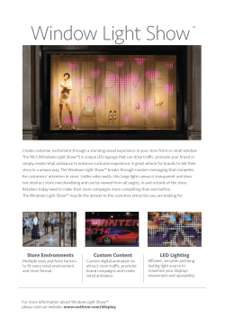
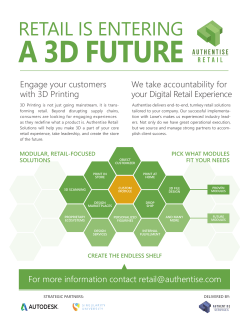
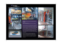

© Copyright 2026