Random Walks: WEEK 4
1
Introduction
Let us first recall an important theorem from last time.
Theorem 1.1 (Stationary distribution). Consider an irreducible Markov chain with transition matrix
P . It has a stationary distribution, i.e., a state distribution π ∗ satisfying π ∗ = π ∗ P , if and only if the
chain is positive-recurrent.
Let π (n) denote the state distribution of the Markov chain at time n. We are interested in the following
question: for any given initial distribution π (0) , does it hold that π (n) −→ π ∗ ?
n→∞
2
The ergodic theorem
Recall that a Markov chain is said to be aperiodic if GCD{n : pii (n) > 0} = 1 for any state i.
Definition 2.1 (Ergodicity). A chain is said to be ergodic if it is irreducible, aperiodic and positiverecurrent.
We will prove the following theorem.
Theorem 2.2 (Ergodic theorem). An ergodic Markov chain admits a unique stationary distribution π ∗
by Theorem 1.1. This distribution is also a “limiting distribution” in the sense
(n)
lim πi
n→∞
= πi∗ , ∀i ∈ S
Remark 2.3. The state distribution is given by π (n) = π (0) P n at any finite time n. The above theorem
implies that the limiting distribution does not depend on the initial distribution π (0) as n → ∞.
We give an example before starting with the proof.
Example 2.4 (Aperiodicity matters). Consider the following Markov chain with two states {0, 1}:
p
1−p
0
1
1−q
q
It is easy to show that the stationary distribution π ∗ satisfying
p
∗
∗
∗ 1−p
π =π P =π
q
1−q
q
p
has the unique solution π ∗ = q+p
, q+p
. As a result of Theorem 2.2, this Markov chain has the limiting
distribution π ∗ for any initial distribution if it is ergodic (i.e. irreducible, aperiodic, postive-recurrent).
The caveat here is that the assumption on the aperiodicity of the Markov chain is not always satisfied
for all p and q.
Suppose p = q = 1 and the initial distribution π (0) = (P{s = 0}, P{s = 1}) = (0, 1), meaning the chain
starts in state 1 with probability one. This Markov chain is not aperiodic. Indeed, we have in this case
1
π (1) = (1, 0), π (2) = (0, 1), π (3) = (1, 0) and so on. We see that state 1 only has even return times, i.e.
GCD{n : p11 (n) > 0} = 2, thus the chain is periodic with period 2. As a consequence, Theorem 2.2
does not apply to this Markov chain in this case. In fact, one can show that for any initial distribution
π (0) = (α, β) with α + β = 1, the Markov chain does not converge to the stationary distribution 12 , 12
unless α = β = 21 .
3
Preliminary tools for the proof
The proof of the ergodic theorem we give here relies on the notions of total variation distance and coupling
that we must first define.
3.1
Total variation distance
Definition 3.1. Let µ and ν be two probability distributions on the same state space S. The total
variation distance d(µ, ν) is defined as
d(µ, ν) = kµ − νkT V = sup |µ(A) − ν(A)|
A⊂S
Remark 3.2. The following statements can be deduced from the definition above:
1. 0 ≤ kµ − νkT V ≤ 1
P
2. kµ − νkT V = 12 j∈S |µ(j) − ν(j)|
3. d(µ, ν) is a distance metric, hence it satisfies the symmetry, non-negative and triangle inequalities.
Example 3.3. Consider two random variables X ∼ N 1, 12 and Y ∼ N (2, 1). The total variation
distance between X and Y is kX − Y kT V ≈ 0.458, which is obtained by choosing A = [−0.29, 1.62].
A
3.2
3.2.1
Coupling
Coupling of random variables
Definition 3.4. Let µ and ν be two probability distributions over S. A coupling between µ and ν is
a pair of random variables (X, Y ) with joint distribution P(X = i, Y = j) over S × S such that the
2
marginals of X and Y are µ and ν. In other words,
X
µi = P(X = i) ≡
P(X = i, Y = j)
j∈S
X
νj = P(Y = j) ≡
P(X = i, Y = j)
i∈S
Example 3.5. We flip a fair coin twice and assign the outcome of each toss to the random variables µ
and ν respectively: µi = νi = 21 , i ∈ {0, 1}.
The two distributions of the random variables (X, Y ) below are couplings of µ and ν:
1. P{X = i, Y = j} = 1/4, (i, j) ∈ {0, 1}2
2. P{X = 0, Y = 0} = P{X = 1, Y = 1} = 1/2
P{X = 1, Y = 0} = P{X = 0, Y = 1} = 0
Proposition 3.6 (Coupling and total variation). Let µ and ν be two probability distributions on S.
Then
kµ − νkT V = inf P {X 6= Y } ,
(X,Y )
where inf (X,Y ) means the infimum on all possible couplings (X, Y ) of µ and ν.
In fact we will only need a weaker variant of this proposition, namely
kµ − νkT V ≤ P {X 6= Y } ,
for any coupling (X, Y ) of µ and ν.
Proof. We will prove the weaker bound.
Let A be any subset of S. We have
µ(A) = P (X ∈ A) = P (X ∈ A, Y ∈ A) + P (X ∈ A, Y ∈ Ac )
ν(A) = P (Y ∈ A) = P (X ∈ A, Y ∈ A) + P (X ∈ Ac , Y ∈ A) ,
hence
µ(A) − ν(A) = P (X ∈ A, Y ∈ Ac ) − P (X ∈ Ac , Y ∈ A)
≤ P (X ∈ A, Y ∈ Ac )
≤ P (X 6= Y )
By symmetry we also have
ν(A) − µ(A) ≤ P (X 6= Y ) .
Thus we get
|µ(A) − ν(A)| ≤ P (X 6= Y )
Moreover, since we did not impose any particular condition on A, we can take the supremum of the LHS,
which gives kµ − νkT V ≤ P (X 6= Y ).
3
3.2.2
Coupling of Markov chains
Let (Xn , n ≥ 0) and (Yn , n ≥ 0) be two Markov chains on the same state space S having initial
distributions π (0) = µ and π (0) = ν respectively. We also assume that both processes have the same
transition matrix P (though this condition can be relaxed).
Definition 3.7. We say that the process ((Xn , Yn ), n ≥ 0) on the state space S × S is a coupling of
Markov chains (Xn , n ≥ 0) and (Yn , n ≥ 0) if the marginals of (Xn , Yn ) are the processes (Xn , n ≥ 0)
and (Yn , n ≥ 0) respectively. In other words,
X
(µP n )i = P (Xn = i) ≡
P (Xn = i, Yn = j)
j∈S
n
(νP )j = P (Yn = j) ≡
X
P (Xn = i, Yn = j)
i∈S
Example 3.8 (Statistical coupling). Consider the processes (Xn , n ≥ 0) and (Yn , n ≥ 0) defined previously. We define the coupling ((Xn , Yn ), n ≥ 0) on the state space S × S such that the initial distribution
(0)
is given by µ ⊗ ν (i.e., πi,j = µi νj ) and the transition matrix is P ⊗ P (i.e., pi,j−→k,l = pi→k pj→l ).
What does statistical coupling represent? We can picture it as the evolution of two clouds through time
in a statistically identical way when starting at two different points.
To verify that this is a valid coupling, we must check that (µP n )i and (νP n )j are the marginals of
(n)
n
((µ ⊗ ν) (P ⊗ P ) )i,j = πi,j , ∀n ≥ 0. This can be proved by induction (the base case n = 1 is shown
below):
X (0)
X
(1)
(1) (1)
πk,l =
πi,j pi,j−→k,l =
µi νj pi→k pj→l = πk πl
i,j∈S
X
l∈S
(1)
πk,l
=
(1)
πk
i,j∈S
X
(1)
πl
=
(1)
πk
= (µP )k
l∈S
Example 3.9 (Grand coupling). Let two random walks (Xn , n ≥ 0) and (Yn , n ≥ 0) be defined on the
following state space:
1/2
1/2
1/2
1/2
1/2
···
0
1/2
1/2
N
1/2
1/2
1/2
To decide the next state of both processes, we toss a fair coin labeled {±1} and move both processes
together either one state forward or backward. In the event a process reaches states 0 or N , it takes the
self-loop if the coin gave −1 or +1 respectively.
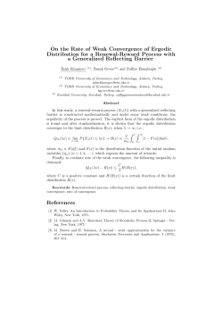
If X0 = 3 and Y0 = 4, such a walk would look like the following (with N = 5):
4
5
4
3
2
1
0
identical movements
τcouple
when chains meet,
they stay together
We see that at a certain point in time both processes coalesce and remain so forever. We will call this
time the coupling time τcouple :
τcouple = inf {n ≥ 1 : Xn = Yn }
4
A proof of the ergodic theorem
To prove the ergodic theorem, we use a mixture of the statistical coupling and grand coupling techniques
seen previously:
Let (Xn , n ≥ 0) and (Yn , n ≥ 0) be two Markov chains with transition matrices P and initial distributions
X0 ∼ µ and Y0 ∼ ν. We define the coupled process (Zn = (Xn , Yn ), n ≥ 0) with the following properties:
1. Z0 ∼ µ ⊗ ν.
2. As long as Xn and Yn have not coalesced, Zn ’s transition matrix is given by P ⊗ P : Zn is in a
statistical coupling scheme.
3. Once Xn = Yn , we switch to a grand coupling scheme: Xm = Ym , ∀m ≥ n.
5
S
Xm = Ym
Y0
X0
n
τcouple
grand coupling:
moves are generated
by a common
source of randomness
statistical coupling:
moves are i.i.d
We will see that when Xn and Yn are ergodic, P (τcouple < ∞) = 1.
The following lemmas and corollary will allow us to prove the theorem.
Lemma 4.1. Let Xn , Yn and Zn be defined as before. Then
kµP n − νP n kT V ≤ P (τcouple > n)
Corollary 4.2. Let (Xn , n ≥ 0) be an irreducible and positive-recurrent Markov chain. The stationary
distribution π ∗ satisfies for any initial distribution π (0)
kπ ∗ − π (n) kT V ≤ P (τcouple > n)
Proof. In Lemma 4.1, take ν = π (0) any arbitrary initial distribution and µ = π ∗ (which exists and is
unique by Theorem 1.1). We get
kµP n − νP n kT V = kπ ∗ P n − π (n) kT V = kπ ∗ − π (n) kT V ≤ P (τcouple > n)
Lemma 4.3. Let (Xn , n ≥ 0) and (Yn , n ≥ 0) be two ergodic Markov chains. Then
P (τcouple > n) −→ 0
n→∞
We are now ready to prove the ergodic theorem.
Proof. (Ergodic theorem). The corollary of Lemma 4.1 implied
kπ ∗ − π (n) kT V ≤ P (τcouple > n)
6
Combining the statement above with Lemma 4.3 gives
lim kπ ∗ − π (n) kT V = 0,
n→∞
which implies the pointwise limit (take the set A = {i} in the definition of the total variation distance)
(n)
lim πi
n→∞
5
= πi∗ , ∀i ∈ S
Proofs of lemmas
We present the detailed proofs of the previously used lemmas in this section.
5.1
Proof of Lemma 4.1
Consider the two probability distributions µP n and νP n at time n. Take the coupling (Xn , Yn ) of µP n
and νP n : this is a valid coupling because by construction
P (Xn = i) = (µP n )i
P (Yn = j) = (νP n )j
By Proposition 3.6, we have
kµP n − νP n kT V ≤ P (Xn 6= Yn )
But the event (Xn 6= Yn ) is equivalent to (τcouple > n) (by the mixed statistical coupling/grand coupling
construction), which proves the lemma.
5.2
Proof of Lemma 4.3
The coupled process (Zn = (Xn , Yn ), n ≥ 0) has the following properties:
• The chain Z is a Markov chain with the transition probability given by
pij→k` = P{Zn+1 = (k, `)|Zn = (i, j)}
= pik pj`
where pik = P{Xn+1 = k|Xn = i}. This fact is easy to verify using the Markovity and independence
of X and Y (in the statistical coupling stage).
• The chain Z is irreducible.
Proof. Using the irreducibility and aperiodicity1 of (Xn , n ≥ 0), we show in the Appendix that
(Xn , n ≥ 0) satisfies the following property:
∀i, j ∈ S, ∃N (i, j) such that ∀n ≥ N (i, j), pij (n) > 0
Obviously (Yn , n ≥ 0) also satisfies this property. Now for any i, j, k, ` ∈ S, choose m > max{N (i, j), N (k, `)}.
We will have
P{Zm = (j, `)|Z0 = (i, k)} = pij (m) pk` (m) > 0
1 We
remark that this is the only place where aperiodicity is used in the proof of the ergodic theorem.
7
• The chain Z is positive-recurrent.
Proof. By assumption (Xn , n ≥ 0) and (Yn , n ≥ 0) are irreducible and positive-recurrent, hence by
Theorem 1.1 both have stationary distributions π ∗ . Now define a distribution ν ∗ on S × S as
∗
νi,j
= πi∗ πj∗
(i, j) ∈ S × S
Using the fact that π ∗ is a stationary distribution for (Xn , n ≥ 0) and (Yn , n ≥ 0), it is easy to
∗
check that νi,j
defined above is indeed a stationary distribution for the chain (Zn , n ≥ 0), i.e.
∗
νi,j
=
X
∗
νk,l
pk`→ij
k,l∈S
Now use Theorem 1.1 again: since Z is irreducible and has a stationary distribution, it must be
positive-recurrent.
Let Z0 = (X0 , Y0 ) = (i, j) and define
Ts = min{n ≥ 1 : Zn = (s, s)}
for some s ∈ S. In words, this is the first time the trajectories of (Xn , n ≥ 0) and (Yn , n ≥ 0) meet at
state s when they start at i and j.
Let m be the smallest time such that pss→ij (m) > 0. By irreducibility we know that a finite such time
exists. This means that the event that the chain goes from (s, s) to (i, j) has non-zero probability. Now,
we claim that the following inequality holds:
pss→ij (m) · (1 − P(Ts < ∞|Z0 = (i, j)) ≤ 1 − P(Ts < ∞|Zn = (s, s))
The RHS is the probability that Z leaves (s, s) and never returns; LHS is the probability that Z goes
from (s, s) to (i, j) in the least number of steps,2 then leaves (i, j) but never returns to (s, s). Obviously
the event of the LHS is included in the event of the RHS (the event of the LHS implies the event of the
RHS). Thus the probability of the LHS is smaller than the probability of the RHS.
The RHS equals zero because Z is recurrent and the first term on the LHS is non-zero because Z is
irreducible. This means we must have
1 − P(Ts < ∞|Z0 = (i, j)) = 0
which proves the lemma.
6
Appendix
In the proof of irreducibility of (Zn , n ≥ 0) we made use of the following technical statement:
Lemma 6.1. Let (Xn , n ≥ 0) be irreducible and aperiodic. Then
∀i, j ∈ S, ∃N (i, j) such that ∀n ≥ N (i, j), pij (n) > 0
Notice that this is stronger than pure irreducibility because we want pij (n) > 0 for all large enough n
(given i, j). This is why aperiodicity is needed. The proof is slightly technical (and has not much to do
with probability); but we present it here for completeness.
2 Here
“least number of steps” ensures the walk does not come back to (s, s) when it goes from (s, s) to (i, j).
8
Proof. For an irreducible aperiodic chain we have for all states GCD{n : pjj (n) > 0} = 1. Thus we can
find a set of integers r1 , . . . , rk such that pjj (rk ) > 0 and GCD{r1 , . . . , rk } = 1.
Claim: for any r > M with M large enough (depending possibly on r1 , . . . , rk ) we can find integers
a1 , . . . , ak ∈ N that are solution of
r = a1 r1 + · · · + ak rk
This claim will be justified at the end of the proof not to disrupt the flow of the main idea.
Since the chain is irreducible, for all i, j we can find some time m such that pij (m) > 0. By the ChapmanKolmogorov equation we have
X
pij (r + m) =
pik (m)pkj (r)
k∈S
≥ pij (m)pjj (r)
Using Chapman-Kolmogorov again and again,
pjj (r) = pjj (a1 r1 + · · · + ak rk )
X
=
pj`1 (a1 r1 )p`1 `2 (a2 r2 ) · · · p`k j (ak rk )
`1 ,··· ,`k ∈S
≥ pjj (a1 r1 )pjj (a2 r2 ) · · · pjj (ak rk )
≥ (pjj (r1 ))a1 (pjj (r2 ))a2 · · · (pjj (rk ))ak
We conclude that
pij (r + m) ≥ pij (m)(pjj (r1 ))a1 (pjj (r2 ))a2 · · · (pjj (rk ))ak > 0
We have obtained that for all r > M (with M large enough), we have pij (r + m) > 0. Thus we have that
pij (n) > 0 for all n > N (i, j) ≡ M + m. Note that in the above construction M depends on j and m
depends on i, j.
It remains to justify the claim. For simplicity we do this for k = 2. Let GCD(a, b) = 1. We show that
for c > ab the equation c = ax0 + by0 has non-negative solutions (x0 , y0 ). If we were allowing negative
integers this claim would follow from B´ezout’s theorem. But here we want non-negative solutions (and
maybe that we don’t remenber B´ezout’s theorem anyway?) so we give an explicit argument.
Take c = ax + by (mod a). Then c ≡ by (mod a). Since a and b are coprime, the inverse b−1 exists (mod
a), so y ≡ b−1 c (mod a). Take the smallest integer y0 = b−1 c (mod a) and try now to solve c = ax + by0
for x. Note that c − by0 > 0 because c > ab. Note also that c − by0 is divisible by a (since y0 − b−1 c ≡ 0
(mod a)). Therefore doing the Euclidean division of c − by0 by a we find x0 non-negative and satisfying
c − by0 = ax0 . We have thus found our solution (x0 , y0 ).
9