
Latest draft
MEKONG ECONOMIC RESEARCH NETWORK DOES THE INFORMAL ECONOMY MITIGATE POVERTY AND HOW DOES IT WORK? THE CASE OF VIETNAM Nguyen Thi Minh Hieu*1 Nguyen Thi Huong Giang* Vu Thi Minh Ngoc** Nguyen Viet Duc* Truong Tan Quan* * Hue College of Economics, ** Vietnam Forestry University December 2014 1 Corresponding authors: Nguyen Thi Minh Hieu: [email protected], Nguyen Thi Huong Giang: [email protected], Vu Thi Minh Ngoc : [email protected], Nguyen Viet Duc : [email protected], Truong Tan Quan : [email protected] 1 Abstract This paper examines the impacts of income from informal employment and informal sector employment on poverty in Vietnam to determine whether the informal economy is an accelerator or a decelerator of poverty. Using data from the 2010 Vietnam Household Living Standard Surveys, we take into account different scenarios of job movement and find that (1) if informal wage workers and informal selfemployed workers are unemployed, then poverty rates will increase by 11 per cent and 7 per cent, respectively; (2) working in agriculture instead of in informal household business leads to increased poverty; and (3) the impact of job formalization on poverty is negligible. Moreover, informality is also associated with the improvement of some nonmonetary indicators of living standard, such as housing and access to national electricity or tap water and having voluntary health care insurance. In the econometric analysis tackling the endogeneity problem, we apply IV Probit and IV quantile models and suggest that informal household business is negatively associated with household poverty, while informal wage activities help reduce household poverty. The impact of informality on household income is stronger in poorer groups and insignificant in the richest class. JEL classification codes: O17, I3 Keywords: informal economy, poverty 2 Acknowledgements This paper was prepared for Mekong Economic Research Network (MERN) conducted by Centre for Analysis and Forecasting (CAF) of the Vietnam Academy of Social Sciences (VASS) with financial support from the International Development Research Centre (IDRC), Canada. We are especially thankful to Dr. Laure Pasquier-Doumer for her helpful comments as the advisor of our research team. We also thank Ms. La Hai Anh and Mr. Nguyen Minh Thai for their advices and supports at the initial stage of this project. This study is benefited from comments of participants in the 1st Networking in Hanoi, Vietnam; 2nd Networking in Vientiane, Laos and 3rd Networking in Phnom Penh, Cambodia. 3 I. Introduction According to Cling et al. (2010), the informal economy in Vietnam will continually maintain its considerable contribution to the country’s employment and income for the coming years. The informal economy is normally associated with poor, unproductive and excluded workers and its significance has varied in different economic periods (Gërxhani, 2004). However, the interpretation of the influence of the informal economy on poverty depends on the adopted theoretical framework. Some economists are in line with the more pessimistic point of view – they assert that the effect of informality on poverty reduction is negative and the informal economy perpetuates poverty. Nevertheless, the larger part of the literature pursues an optimistic sentiment and concludes that there is a positive linkage between informality and poverty alleviation. This paper aims to examine the impact of the informal economy on poverty in Vietnam to determine which view is suppored by an empirical study. We use data from the Vietnamese Households Living Standard Survey (VHLSS) carried out in 2010 to first draw a picture of the informal economy, poverty and the relationship between the two using descriptive statistics. We then estimate the influence of informal income on a household’s poverty and economic status. However, this estimation raises a methodological difficulty: The endogeneity of informal income resulting from reverse relationships between poverty and informality and the unobserved characteristics of household members. To address this, we use the average time to get the business license and the average share of labor training cost in the total cost of the enterprises as instrumental variables for informality. In particular, the IV Probit models are employed to investigate the impact of informal income on the probability of the household being poor. At the same time, IV quantile regressions are used for the concern that the responsiveness of household income on informal earnings is not equal across levels of household income. The paper has seven sections. After the introduction, Section 2 provides a selective overview of the existing literature. Section 3 defines the main concepts and the data 4 used in this paper. Section 4 explores the relationship between informality and poverty through descriptive statistics. The next section discusses research methodology. Section 6 provides empirical results, while the last section contains the conclusions and some policy implications. II. Literature review Recognition and characteristics of the informal economy The informal sector of the economy was first introduced by Hart (1970, 1973), but only covered self-employment in developing countries. In a report on Kenya by the International Labor Organization (ILO) in 1972, the informal sector was then recognized as the activities of the poor who were working very hard but were not recognized, recorded, protected or regulated by the public authorities. Later, De Soto (1989) asserted that legal status was the main element distinguishing between the informal and formal sectors. Until now, the informal sector has been defined in various ways (ILO 1972; Weeks 1975; Bromley 1978; Castells & Portes 1989; International Conference of Labor Statisticians 1993; Tokman 2001; Pratap & Quintin2006). However, in 2002, a broader concept of ‘informal economy’ was adopted and this led to the informal sector being recognised as an economy wide phenomenon. The definition of the informal economy acknowledges not only unregistered and unrecognized firms, but also workers who are in an uncertain and volatile situation (ILO, 2013). In other words, the informal economy includes both the informal sector and informal employment. Informal employment is a broader concept which also includes employment of an informal nature in formal enterprises, as well as wage and self-employment in informal enterprises and households businesses. In general, the informal sector is characterized by low productivity, low investments, poor working conditions, long and uncertain working hours, low wages, poor market conditions and poor institutional support (Agarwal and Dhakal, 2010). Furthermore, the sector is defined by its informal labour status, high tax evasion, small size of activities, lack of professional status, lack of regulation or registration of an activity 5 and absence of contribution to GNP accounts are all sub-criteria of the economic pattern describing the informal sector (Harding and Jenkins 1989, Renooy 1990 and the ILO 1972). Meanwhile, informal employment often means low earnings and limited access to legal and social protection and resources (ILO, 2010). The informal employment sector is normally occupied by the most vulnerable in the labor markets, including women, the young and elderly, migrants and low-skilled workers. These workers have limited bargaining power and representation, as well as have little chance to increase their socio-economic standing in the future. Informal employment, when referring to individual businesses or micro and small enterprises, is often synonymous with low growth and productivity, and limited access to mainstream resources (ILO, 2013). The determinants of entering the informal economy and predictions on the development of the informal economy According to Friedman et al (2000), there are two main theories on the determinants of entering the informal economy. The first theory states that the most important factor affecting the decision to enter the informal economy is taxation. High tax rates may reduce firms’ profits, whereas operating in the informal economy helps retain their profits. The second theory states that the key determinants are the political and social institutions that govern the economy. Bureaucracy, corruption, the burden of regulation, and a weak legal system are all factors that can be attributed to the rise of informal economy (Friedman et al, 2000; Strabu, 2005). Overall, the view is that countries with lower quality institutions or heavier burden of regulation are also associated with a larger informal sector. In addition, other studies show that low startup costs are a key determinant in entering informal economy (Strabu, 2005; Antunes & Tiago, 2007; Dougherty & Escobar, 2013). Being formal entails significant costs including direct costs such as registration and license fees, and indirect costs such as the opportunity cost of time spent becoming formal. Djankov et al. (2002) provide preliminary evidence that 6 countries with heavier regulation of entry have larger informal sectors. Furthermore, regulations including labor market rigidities, including minimum wage, dismissal costs and other employment laws meant to protect workers are potential determinants of informality (Strabu, 2005). Most of the studies analyzing the informal economy in the short run show that it naturally tends to decline over time, especially in developed countries (GutiérrezRomero, 2010). However, there is a contrary prediction for developing countries where informality remains an important phenomenon and experiences marked increases (Perry et al, 2007). Linkage between informality and poverty Although the importance of the informal economy is now widely acknowledged, its linkages with poverty are still controversial. As far as a connection between poverty and informality is concerned, we can divide the literature into two groups of ideas, namely the pessimistic and optimistic groups. In the pessimistic point of view, the informal sector consists of marginal and subsistence activities, where the productivity and earnings of its participants remain low. Informal workers enjoy little social protection, and working conditions are very poor (ESCAP, 2006). Therefore, the informal sector perpetuates poverty and the effect of informality on poverty reduction is negative. In addition, Timofeyev (2013) uses the latest available data from the Russian Federal State Statistics Service to calculate labor income scales for the poor in the informal sector, and compares them to average wages in the formal sector and with the official poverty line of Russia. The study concludes that while the informal sector is a factor of social stability in a postsocialist transition economy, it cannot, however, alleviate poverty. The second view is that not everyone working in the informal sector is poor, and there is a positive link between informality and poverty alleviation. A number of empirical studies support this optimistic sentiment. Admittedly, the vast majority of informal participants have low incomes and live below or close to the poverty line 7 (ESCAP, 2006). However, without the informal sector, the intensity of poverty would be much higher. Cartaya (1991), as cited in Orlando (2001), emphasizes that in Venezuela, a significant portion of household income comes from the informal sector, for both poor and non-poor households. The author finds an important relationship between poverty intensity and informality, given that the families in extreme poverty earn the greatest part of their income from the informal sector. Additionally, Orlando (2001) shows that the increase in the rate of informal earnings is lower than the increase in the rate of employment. This means that the incidence of poverty is higher in the informal sector than in the formal sector. Hence, he suggests that a strategy to reduce poverty should be to increase productivity and wage levels in the informal sector through improving education, working experience , and capital access for informal employees. Agarwal & Dhakal (2010) show that in developing countries, the main reason for joining the informal sector is to safeguard poor and marginalized from poverty and unemployment. Based on Nepal’s experiences, Agarwal and Dhakal (2010) also suggest that the informal sector is a good source of livelihood for poor and marginalized groups. They prove that earnings from the informal sector have had a strong impact on the households’ livelihood. Surprisingly, without the earnings from the informal sector, more than 94 per cent of households in Chitwan district of Nepal were drowned in poverty, but due to the income generated from the informal sector activities there has been a remarkable shift and only 12.9 per cent of households remain in poverty, while 46 per cent of the households have been able to join the middle income and high income classes. With regard to the linkage between informality and poverty in Vietnam, Cling et al. (2009) are the only ones to examine this linkage. They find that, excluding agriculture employment, the poor households are more likely to be involved in the informal economy, and this increases from 31 per cent at the richest quintile to 87 per cent at the poorest in 2004. However, for the different economic regions, the informal rate is not highest in the poorest region. This is explained by the fact that informality concentrates in developed, urban and suburban areas. They conclude that although 8 poverty reduction is an important policy question in Vietnam, the linkage between informality and poverty is almost completely ignored. Cling et al (2011) further emphasize that targeted policies should be designed and implemented to deal with the fact that poverty is progressively changing and is now more of an urban and informal phenomenon. The evidence on the role of the informal economy in poverty reduction in many developing countries combined with the lack of studies on the relationship between the informal economy and poverty in Vietnam are an clear gap that this study fills. Vietnam’s poverty and informality Vietnam has made impressive achievements in poverty reduction in recent years. These achievements can be seen in three dimensions: the poverty rate, the characteristics of poverty, and other non-monetary indicators of poverty. The poverty rate decreased consistently, from 58 per cent in early 1990s to 14.5 per cent in 2008 and 12 per cent in 2011 (World Bank, 2013). Around 28 million people are estimated to have been lifted out of poverty over approximately one and a half decades, from 1993 to 2008 (World Bank, 2011). Those who remained in poverty saw their wellbeing considerably improving over this period (World Bank, 2011). The average shortfall of consumption from the poverty line, (as measured by the poverty gap rate) also fell steadily from 18.5 per cent in 1993 to as low as 3.5 per cent in 2008 (World Bank, 2011). The poverty severity rate – which gives higher weight to the poorest among the poor – declined from 7.9 per cent in 1993 to 1.2 per cent in 2008 (World Bank, 2011). The characteristics of Vietnam’s poverty also changed significantly. The average size of poor households declined from 5.2 people to 4.8 people while the dependency ratio dropped from 55 per cent in 1993 to 49.7 per cent in 2008 (World Bank, 2011). Other non-monetary indicators such as access of the poor to basic social services and infrastructures (education, health, electricity, road, water and sanitation, etc.) also demonstrated a very positive trend. 9 With regard to informality, Cling et al, (2011) show that in 2007, the informal sector constituted nearly 11 million jobs out of all main jobs and around 12.4 million out of main and second jobs. In addition, the informal sector is estimated to contribute 20 per cent of GDP. Sharing a similar view, Nguyen Huu Chi et al (2010), using Labour Force Survey, conclude that informal employment remained a huge proportion – around 80 per cent – of total jobs during the time from 2007 to 2009. This means that in Vietnam only around 9 million workers are covered by the social insurance scheme (which includes mandatory and voluntary social insurance). The informal sector constitutes an important source of employment, accounting for around 30% of jobs in the two major cities of Hanoi and Ho Chi Minh City (Demenet et al, 2010). In addition, informal employment is found beyond the agricultural sector and informal sectors. Most employment in domestic enterprises in some industries such as construction, trade and accommodation can be defined as informal employment in either the formal or the informal sector (Cling et al, 2010). Rand et al (2012), using the Small and Medium Enterprise survey carried out in 2009, observe that average wages are 10 – 20 per cent higher in formal micro firms than in informal micro firms, due to differences in characteristics between the two firm categories such as firm size and location. Meanwhile, Cling et al (2010) use comparative analysis to investigate the similarities and differences between the informal sectors in Vietnam and Africa. The results show that the informal sectors in both countries have many similarities in terms of development level and economic structure. The informal sector is predominant in both Africa and Vietnam; however the author asserts that the Vietnamese informal business is more pessimistic in the medium and long term. III. Definition and Data Informality and the Vietnam Household Living Standard Survey 2010 In Vietnam, an operational definition of informality has been developed by the General Statistics Office (GSO) in 2007. According to the GSO, the informal sector is defined as all private unincorporated enterprises that produce at least some of their goods and services for sale or barter, that do not have a business license, and that are engaged in 10 non-agricultural activities. Employment in the informal sector is referred to as informal sector employment (ILO, 2002). The informal employment is operationally defined as unpaid family work and wage or salaried work without social security in nonagricultural sectors. Therefore, it is comprised of employment in the informal sector as well as parts of employment in the formal sector. The Vietnamese Household Living Standards Surveys (VHLSS) are unique national surveys containing information about both employment and living standard and thus they are the most appropriate data set to examine the relationship between the informal economy and poverty. The GSO has conducted the VHLSS regularly every two years from 2002 to 2012. The survey sample covers 64 provinces and 8 regions and is representative at the national and regional levels, in both rural and urban areas of Vietnam. Its contents include basic demography, education and health status, occupation, income and expenditure of all household members, non-farm business, fixed assets, durable, housing and household participation in poverty reduction programs. The data set is sufficiently informative about jobs and household income enabling them to be categorised into poor or non-poor group. The most updated and available survey, 2010 VHLSS, is used in this paper. According to the GSO’s definition, 2010 VHLSS data allows defining households running their own business without a business license (unregistered business) as informal sector employment and household members who work for a wage but do not have social security as informal employment. However, it is worth noting that both informal sector employment and informal employment derived from 2010 VHLSS data are a part of informal sector employment and informal employment defined by the GSO. In particular, (1) informal sector employment in 2010 VHLSS excludes non-household businesses such as employment in a private enterprise without a business license. Meanwhile (2) informal employment does not include those who work for no wage, (for example, unpaid family employment) due to the unavailability of information on social security. Thus, we adopt the definition of informal workers developed by 11 Nguyen Huu Chi (2010)2: that is, informal workers are those who work for a wage but do not have social security, plus workers who are self-employed in unregisteredhousehold businesses. Agriculture is excluded in both definitions. The relationship between the definitions of informality introduced by the GSO and Nguyen Huu Chi is summarised in the following figure: Informal employment Informal sector employment employment in nonhousehold enterprise without business license employment in household enterprise without business license Informal self-employed workers wage employment without social security non-wage employment without social security Informal wage workers Informal workers Figure 1. Components of informality The two boxes highlighted in Figure 1 are part of informal sector employment and informal employment as included in the GSO’s definition, but excluded in Nguyen Huu Chi’s definition. According to the definition of informal workers, informal income or informal earnings are constructed from two sources. The first source is informal wage earnings generated by informal wage workers. Wage earnings are obtained by summing up the direct wages combined with all the supplementary benefits converted into pecuniary equivalent. The second source is informal self-employed earnings created by informal self-employed workers. These earnings are calculated from household non-farm business. Average earnings of self-employed workers in the household are equal to the total earnings from non-farm household business divided by number of household members working in the business3. 2 Due to the unavailability of social insurance in the VHLSS survey conducted before 2010, Nguyen Huu Chi, et al. (2010) use the criteria of health care insurance to define informal wage workers. 3 household members whose are aged 15 years or more, and have worked for the last 12 months in the household business 12 2010 VHLSS’s biased measure of informality As mentioned, the informality calculated using 2010 VHLSS is a part of the informality defined by the GSO. The 2010 VHLSS’s biased measurement of informality can be estimated using the 2010 Labour Force Survey (2010 LFS). The 2010 LFS reveals that the rates of informal employment and informal sector employment are 62.2 and 42.64 per cent, respectively. Meanwhile, the percentages of informal wage workers and self-employed workers in the VHLSS are 36.4 and 22.5, respectively. Thus, the 2010 VHLSS captures 69 per cent of informal employment and 53 per cent of the informal sector employment. The 2010 LFS also shows that those excluded from the informal wage data are more likely to be female workers, belonging to a minority, or of older age, while those excluded from informal sector employment are more likely to be male, belong to a majority, of younger age and have a higher level of education (See appendix A0). Poverty In Vietnam, poverty rates are calculated by the GSO based on the VHLSS data; two different types of poverty rates are reported. One is calculated using income and the other is based on expenditure. This paper uses income poverty rates to examine the contribution of informal workers to the household income. This poverty rate shows the percentage of households with a per capita income below the poverty line, which is 500,000 VND in urban area and 400,000 VND in rural area in 2010. The poverty rate is calculated using the whole income of households, including value of aid, scholarships, rewards from education and healthcare, salaries/wages of household members, income from renting out land and house, agriculture production and business outside agriculture and other revenues. 4 If agriculture is excluded then the rates of informal employment and informal sector employment are 62.2 and 42.64 percent, respectively. If agriculture is included, the rates are 82.4 and 42.3 percent, respectively. 13 IV. Linkage between poverty and informality in Vietnam Informal employment and informal income in Vietnam in 2010: some statistical indicators Table 1 below provides information about the income and employment structure in the whole economy, as well as by poverty status, in Vietnam based on the VHLSS 2010. It can be seen that the informal sector is an important source of both employment and income for households in Vietnam. The percentage of informal workers, as a share of total workers, accounts for more than 30 per cent while informal income contributes to about 26 per cent of household income. In contrast, around 23 per cent of total employment and 21 per cent of household total income are derived from formal activities. The agriculture sector is still the main contributor to total employment and household total income, with rates of 47 per cent and 26 per cent, respectively. The poor group relies heavily on agriculture activities in terms of both employment and income sources, and the proportion of formal earnings in their total household income is negligible. One possible reason for this is that the poor are likely to face more disadvantages than the non-poor in the process of seeking formal jobs. In addition, the contribution of informal activities to household employment and income is also modest, due to the dominance of agriculture. Notably, in the non-poor group, nearly half of employment originates from the agricultural sector. However, the contribution of earnings from informality, formality, agriculture and other sources to the total income of the non-poor households is almost equal. For the whole population, the proportion of employment from informal sources always exceeds that from formal ones in terms of both wage workers and the selfemployed. Wages play a more important role than self-employment income in the share of total income of all households. As can be seen in the last column of Table 2, if agricultural employment and income are excluded, informal workers account for about 59 per cent of non-agricultural 14 employment and their informal earnings comprise 32 per cent of non-agricultural income of households. Of this total contribution of informal income and employment, informal wage-activities contribute a higher proportion in terms of both employment and income in comparison with informal self-employed activities for the whole population. Table 1. Household employment and income structure by poverty status Poor households Non-poor households All households Informal self-employed workers 3.0 13.2 12.3 Informal wage workers 6.4 19.3 18.2 Formal self-employed workers 1.1 8.0 7.4 Formal wage workers 1.5 16.9 15.5 Agriculture workers 88.0 42.6 46.6 Total 100 100 100 2,353 19,264 21,617 Informal self-employed earnings 3.8 11.4 10.7 Informal wage earnings 6.9 16.1 15.3 Formal self-employed earnings 1.3 7.3 6.7 Formal wage earnings 1.2 15.5 14.3 Agriculture earnings 51.6 24.0 26.4 Others5 35.3 25.8 26.6 Total 100 100 100 Employment structure (%) Number of observations Income structure (%) Source: Author’s calculation from VHLSS 2010. 5 The category ‘other sources of income’ represents all sources that households received in the last twelve months in cash or in kind. They include income from household members not living with the household or nonhousehold members within the country, remittance from overseas, gifts and money presented after weddings and other cultural activities, the pension or subsidy from the Government or charity organizations, money from insurance, savings interest and other kinds of rent. 15 In particular, the data reveal that the poorest group suffers a double disadvantage, which is underemployment coupled with low earnings. While the share of informal workers in non- agricultural employment in this group is the highest among the population, income from informal activities in this group is the lowest among the five quintiles. This can be attributed to the characteristics of informal workers, as pointed out by Agarwal and Dhakal (2010): low productivity, low investment, low earnings and poor institutional support. In contrast, the middle income classes benefit most from informal activities, especially for the Quintile 3, with the highest proportions of informality. Table 2. Proportion of informality in household’s income and main features of informalworkers, by quintile 1st 2nd 3rd 4th 5th Total % Inf. self-employed worker in nonagri employment of hh. 25.3 24 27.7 23 16.8 22.5 % Informal wage-worker in nonagri employment of hh. 56.7 55 44.3 32.8 17.8 36.4 % Inf. self-employed earning in nonagri income of hh. 7.9 12.4 17.1 16.4 12.1 13.3 13.4 26.1 26.1 19.8 9.5 18.7 9,069 14,941 19,108 28,926 51,666 27,617 11,766 17,180 21,051 25,087 34,366 22,493 Average monthly working hour of inf. self-employed workers 196 206 208 210 218 209 Average monthly working hour of informal wage workers 214 221 222 214 209 217 Quintile % Informal wage-earning in nonagri incomeof hh. Average yearly income of inf. self-employed worker (1000 VND) Average yearly income of inf. wage workers (1000 VND) Source: Author’s calculation from VHLSS 2010. Keeping informal wages and informal self- employed activities separate, it can be seen that the contribution of informal self-employed workers and informal wage workers to total non-agricultural employment in the richest group are almost equal. In contrast, for the two poorest classes this rate is more than double for the informal 16 wage workers when compared to the informal self-employed workers. There is a similar pattern for income. Hence, it can be said that informal wage activities are dominant for the poorest classes when compared to informal self-employed activities, in terms of both employment and income. Regarding average yearly income, in general, informal income is higher in the richer group and the earnings of informal self-employed workers are higher than those of the informal wage workers. However, yearly earnings of informal wage workers are higher for the first three quintiles, while informal self-employed workers’ earnings are dominant for the 4th and the 5th quintiles. In addition, there is a large difference in average yearly income between the quintiles. The average yearly income of the informal self-employed workers in the 5th quintile is nearly double that of those in the 4th quintile and six times as high as that in the 1st quintile. Similarly, the average income of informal wage workers in the 5 th group triples that in the 1st group. Although the average monthly working hours are similar across quintiles, the poorer groups, on average, receive much lower return from work. The contribution of informal income in poverty alleviation in Vietnam The contribution of informal income to per capita income Table 3. Monthly per capita income of households with members being involved in informal activities Indicators Per capita income in Non-Poor household (1000 VND) Per capita income in Poor household (1000 VND) HH without members in informality HH. with members being informal wage-workers HH. with members being informal selfemployed workers All households 2,024 1,514 1,641 1,801 297 351 330 307 Source: Author’s calculation from VHLSS 2010. The Table 3 shows how the per capita income is in households with informal income. Among the poor group, (a) the households with members working as informal 17 workers are better off than those without any members working as informal workers; and (b) households with members who are informally self-employed have lower per capita income than households with members working as informal wage workers. In contrast, an opposite pattern to (a) and (b) is seen for non-poor group. This result supports the expectation that earnings from informal activities improve living standard of the poor. It also reinforce findings that informal wage workers play more important role than informal self- employed workers in the poor households, as reported in Table 2. The contribution of informal income to poverty rate In order to estimate the contribution of informal income to poverty alleviation, we impose three assumptions, as follows: (i) If informal workers do not work as informal workers, they may be unemployed; (ii) If informal workers do not work as informal workers and their household has enough land, they may move to the agricultural sector; (iii) If informal workers do not work as informal workers and the formal economy has capacity to absorb these workers, they may work in the formal economy. Based on these assumptions and the relevance of employment characteristics among five categories of employees (agricultural workers, informal self-employed workers, informal wage workers, formal self-employed workers and formal wage workers), in this analysis we re-estimate a household’s total income after taking into account the above assumptions. There are five different scenarios, as follows: (1) Informal self-employed workers are unemployed (2) Informal wage workers are unemployed (3) Informal self-employed workers move to agriculture (4) Informal self-employed workers become formal self-employed workers (5) Informal wage workers become formal wage workers. 18 In Tables 4 and 5, we estimate actual poverty rate and poverty index. We also predict these statistical indicators corresponding to the scenarios (1) – (5) to see the impact of informal sector on poverty alleviation in Vietnam. Table 4 shows that with informal income included, the poverty rate is 10.3 per cent and only the 1st quintile suffers from poverty. When the five different scenarios are applied, the poverty rate varies significantly across scenarios and quintiles. In the first two scenarios, the poverty rate is recalculated by excluding informal wage earnings and informal self-employed earnings from per capita income. In these cases, not only the first quintile suffers from high poverty rate, but other quintiles, including richest groups, also fall into poverty. In addition, it is clear that the exclusion of informal wage earnings leads to a higher poverty rate for the whole population as well as in all five quintiles. This shows that the earnings of informal wage workers have a greater impact on the poverty rate than the earnings of informal self-employed workers. Table 4. Poverty rate with different scenarios, by quintile Poverty rate in different scenario (%) Quintiles 1st 2nd 3rd 4th 5th Total 51.40 0.00 0.00 0.00 0.00 10.30 1. Informal wage-workers are unemployed 61.50 22.70 13.90 6.00 2.20 21.30 2. Informal self-employed workers are unemployed 57.00 9.80 9.20 6.10 4.00 17.20 3. Informal self-employed workers move to agriculture 51.46 3.04 2.50 1.65 1.17 11.98 4. Informal self-employed workers become formal self-employed workers 50.18 0.53 0.16 0.00 0.00 10.19 49.39 5. Informal wage-workers become formal wage-workers Source: author’s calculation from VHLSS 2010 1.33 0.21 0.05 0.00 10.21 Actuality Scenario When informal self-employed workers are supposed to move to the agricultural sector in the third scenario, the poverty rate is still higher than currently. However, it 19 is less than the rate in the case that they become unemployed. This can be explained by the fact that agricultural work generally brings an unstable and low income. In the last two scenarios, when informal workers can be formalized, the poverty rates are just slightly lower than the current rate. This can be explained by the fact that informal self-employed workers are those working in unregistered household businesses, these businesses are often small or medium scale, and operate without paying tax. Moving to formal self-employed workers with registered businesses may lead them to suffer from a double disadvantage, arising from both income tax and low competitiveness. Similarly, when informal wage workers become formal wage workers, their overall welfare may improve. However, it is not a strong effect. Because of the main characteristics of informal wage workers (including low education, being low-skilled or unskilled), formalization makes it harder for these workers to compete with formal wage workers in the labor market. However, overall, the households are slightly better off when their members are formally employed. Informal income and poverty index Regarding poverty gap and poverty incidence, both are higher compared to the current values in all scenarios. In the first and second cases, when the informal income is subtracted from the per capita income, the two indicators are both much higher than the current statistics. This implies that without informal income, the population has greater incidence of poverty and their poverty tends to be more severe. In addition, we can see that the poverty gap and poverty incidence are all higher when informal wage workers become unemployed than when informal selfemployed workers are unemployed. This phenomenon reconfirms the conclusion that compared to informal self-employed income, informal wage income has a stronger influence on poverty reduction. If informal self-employed workers can find jobs in the agriculture sector, the poverty index and the poverty incidence are both higher than those in the current case, but 20 not as high as in the first two scenarios. This shows that agricultural work does help to earn money, but the earnings are less than in the case when the work is informal and non-farm. Thus, moving from informal household business to agriculture makes the poor become poorer and sinks a proportion of them to extreme poverty. Table 5. Poverty index6 with informal income included and excluded Poverty Index Poverty index in different scenarios (%) P1 P2 0.0264 0.0102 1. Informal wage-workers are unemployed 0.0884 0.0540 2. Informal self-employed workers are unemployed 0.0661 0.0395 3. Informal self-employed workers move to agriculture 0.0310 0.0121 4. Informal self-employed workers become formal self-employed workers 0.0273 0.0109 5. Informal wage-workers become formal wage-workers 0.0267 0.0103 Actuality Scenario Source: Author’s calculation from VHLSS 2010. In the fourth and fifth scenarios, when informal workers move to the formal sector, the statistics do not change much. This is similar to what happens to the poverty rate and has been explained above. The contribution of informal income to other aspects of life 6 P is an index originally suggested by Foster, Greer, and Thorbecke (1984), the FGT-index. For a continuous income distribution it is given by where z is the poverty line and y stands for income and α = 0, 1, 2. For α = 0 and 1, the FGT-index measures, respectively, the prevalence and the intensity of poverty. For α=2 the FGT-index measures the severity of poverty. 21 Tables 6.1 and 6.2 examine the impact of informality on household living standards in terms of various aspects of life. There are similar results when we look at all households in general and poor households in particular. Table 6.1 . The contribution of informal income to other aspects of life for poor households (in percentages) Indicators Poor hh. Poor hh. with members are Total without informal informal selfmembers in wage employed informality workers workers Housing Permanent house 32 33.84 35.03 32.74 Semi-permanent house 31.49 29.85 34.69 31.42 Temporary and other house 36.51 36.31 30.28 35.84 100 100 100 100 Access to national electricity 86.13 97.17 86.44 87.42 Access to tap water 3.84 9.88 9.02 5.18 Having health insurance 82.3 73.11 76.06 80.69 Kind of insurance Voluntary insurance for students 5.22 10.90 11.31 Other voluntary insurance 1.57 1.81 2.1 1.63 7.6 8.2 5.5 7.5 Total Proportion of children dropping out of school7 6.42 Source: Author’s calculation from VHLSS 2010. It seems that having members involved in informal work would help the households improve some life standard indicators, although the effect is not really significant. For the whole population (Table 6.2), the rates of households having permanent houses, and access to national electricity and tap water are slightly higher in households with members working in the informal sector compared to households without members working in this area. This effect is even stronger for poor households (Table 6.1), 7 The Proportion of children aged between 6 and 18 years old without going to school in all children age between 6 and 18 years 22 especially regarding the ability to access national electricity and tap water. In addition, the proportion of households buying voluntary insurance is always significantly higher for the group of households with a member involved in informal Table 6.2. The contribution of informal income to other aspects of life for the whole population (in percentages) Indicators Housing Household without members in informality Household with members are informal informal selfwage employed workers workers Total Permanent house 48.02 52.32 47.55 49.16 Semi-permanent house 36.24 37.47 42.42 37.66 Temporary and other house 15.75 10.21 10.03 13.18 100 100 100 100 Access to national electricity 95.88 99.55 98.66 97.43 Access to tap water 25.66 28.22 32.08 27.26 Having health insurance 67.58 51.08 54.96 60.50 Kind of insurance Voluntary insurance for students 17.89 27.50 31.54 22.88 Other voluntary insurance 8.54 13.55 17.26 11.28 5.85 7.07 4.53 5.88 Total Proportion of children dropping out of school Source: Author’s calculation from VHLSS 2010. work. However, the coverage of health insurance is lower for households being involved in informal activities. This situation can be explained by the fact that poor households are provided free health care insurance by government. With income from informal activities, a significant proportion of the population shifts into the nonpoor class (10.3 per cent instead of 30.5 per cent of population are poor with and without informal income, respectively). Therefore, these households are no longer 23 provided with free health insurance, so the coverage of health insurance for the whole population may be reduced. Another important indicator that reflects household living standards is the rate at which children drop out of school, but this rate is similar between the two groups of households. V. Methodology For the purpose of exploring the impact of the informal economy on poverty reduction, first a Probit model is applied to examine the responsiveness of one’s poverty situation on earnings from informal sources. Household income is then regressed on informal earnings to find out the contribution of informal earnings to the total income of the household. However, we suspect this contribution is not uniform across all income levels of households. Thus, the quantile regression is employed to explore the variation across the entire distribution of household’s income. Informal wage earnings and informal self-employed earnings are believed to have different impacts on household economic conditions. Thus, these two sources of earnings will be estimated separately in econometric models. Probit model Let Y = 1 if the household is poor and Y = 0 if the household is non-poor. Assuming that the poverty situation of the household depends on an unobservable income index Ii, that is determined by the full set of explanatory variables, X. Thus Ii can be expressed as a linear function of X as follows: I 0 1 X1 2 X 2 ... k X k Assuming that there is a threshold value of I , denoted as I * such that: Y = 1 if I I * Y = 0 if I < I * The threshold I * is a latent variable, determined by I * = I + u with the assumption that u is independent of X and I* is normal distribution. 24 Given assumptions of normality , the probability that I i* is smaller than I is determined by the function F(I) which is the standardized cumulative normal distribution 1 pi p(Y 1| X ) p( I I ) F ( I i ) 2 * 0 1 X1 2 X 2 ... k X k e 1 t2 2 dt 1 12 I 2 f (I ) e 2 where p(Y 1| X ) represents the probability of the occurrence of the event for any value of X. F(I) is the cumulative standardized normal distribution, therefore f(I) which is its derivative is the standardized normal distribution itself: f (I ) 1 12 I 2 e 2 Estimates of the parameters are obtained by maximum likelihood estimation. The marginal effect of Xi is p / X i which is best computed as p dp I f ( I ). i X i dI X i Quantile regression The method of ordinary least squares (OLS) is popularly employed for estimating the parameters in order to explain the relationship between the dependent variable and a set of independent variables. Just as with the classical linear regression model for the conditional mean functions, the quantile regression provides mechanism for estimating models for conditional quantile functions (including conditional median function). In contrast to the parameter estimation of OLS by minimizing a sum of squared residuals, the parameters can be estimated by minimizing a sum of absolute residuals to derive the ‘central tendency’ of the effects from the conditional distribution of median. Median and mean are both very important location measures which characterize the ‘center’ and ‘average’ of distribution respectively; however, they may provide little information about the distribution of tails. For example, two distributions which have the same means could differ in their pattern of distributions such as different variance and skewness. Similarly, since the median can describe the 25 location of distribution to some extent, we have to observe quantiles rather than the median to have a complete understanding of the whole distribution. Quantile regression was proposed by Koenker & Bassett (1978). Consider a sample (yi, xi), i = 1,...,n from a population where xi is an Kx1 vector of regressors. The quantile regression model is postulated as follows: yi xi' ui , where represents the error term such that Quant (ui , | xi ) 0 , where Quant ( yi | xi ) denotes the th conditional quantile of yi given a set of regressors, vector xi. The assumption that Quant (ui , | xi ) 0 implies that only the error term ui , satisfies the assumption that the th quantile of ui , (i.e., yi xi' ) conditional upon the vector of regressors is equal to zero. This assumption is made simply to identify the intercept term in . Thus, Quant ( yi | xi ) xi' where is the vector of parameters. The th (0 1) quantile regression estimator ˆ ( ) is obtained by minimizing the following problem: 1 min yi xi' 1 yi xi' n i: yi xi' i: yi xi' This is normally written as: min yi xi' i where u , known as the check function, is defined as follows: u u if u 0 or u 1 u if u 0 Given , minimizing this function yields the th sample quantile of y. The difficulty in estimation is that the quantile regression estimator ˆ does not have an explicit form. However, the desired estimator ˆ can be obtained by linear programming methods. Standard errors are obtainable by bootstrap methods. 26 The first quartile is obtained by setting = 0.25 and so on. Quintiles are the 20th, 40th, 60th, and the 80th position over the distribution. As is set at any value from 0 to 1, one traces the whole distribution. In conclusion, quantile regressions outline different points of a conditional distribution, which represents a parsimonious way of describing the entire distribution. In addition, they provide much more valuable information in the case that the relationship between the regressors and the dependent variable evolves across its conditional distribution. Potential endogeneity In Vietnam, Article 49 in Decree 43CP promulgated in April 15th 2010 states that households operating their own businesses do not need to register if the business operation generates a low income. Thus, low income is a reason for households not to register their business and to operate it informally. Moreover, it is common sense that poor households do not have sufficient financial resources to invest in their own business. Consequently, they end up with informal activities. These reverse relationships between poverty and informality raise a problem of endogeneity, which leads to inconsistent estimators. Another source of endogeneity is the unobserved characteristics of household members. In particular, members of poor households might suffer more unobserved disadvantage than their counterparts. For example, poor people are rarely equipped with soft skills, and this becomes an obstacle for them to pass the qualification barrier to get formal jobs. In other words, whether a household is poor or not might affect the decision to operate a household business in a formal or informal way and the opportunity to get formal employment for household members. If this is the case, informality is endogenous to household income. Furthermore, other unobserved characteristics (such as having parents as informal entrepreneurs and low ability) could be another potential source of endogeneity, as they might jointly explain informality and poverty. Thus, the assumption of independence between the explanatory variable of informality and the disturbance terms is violated in the model. Therefore the estimated OLS coefficients will be biased and inconsistent. 27 Instrumental variable estimation is an appropriate solution to address the endogenous issue. A valid instrumental variable must satisfy two conditions: it should be (1) highly correlated to the endogenous explanatory variable and (2) uncorrelated to the disturbance term in the equation regression, in which an endogenous explanatory variable appears in the right hand side together with other explanatory variables. Variable construction Dependent variable The dependent variable introduced in the Probit model is a dummy variable defining a poor household, while in the IV quantile regression it is the natural logarithm of a household’s per capita income. Explanatory variables Share of informal income Informal earnings are primary explanatory variables in the model because they help answer the question of whether the informal economy reduces poverty. In particular, the proportion of informal wage earnings and informal self-employed earnings, to the total income of the household are separately introduced in econometric models to distinguish different impacts of these two informal earnings sources on poverty. In the 2010 VHLSS, the total income of households contains wages, aid, income generated from agricultural activities, household businesses as well as from land and houses renting. Household head’s characteristics In the VHLSS, the household head is regarded as the main decision-maker in the household; hence, the characteristics of the household head may shape the household’s economic capacity. Variables of age, age squared, education and vocational training experience (measured by the highest attained qualification) of the head and dummy variables defining a business and agriculture household, male-head household, minority head household and the head with a spouse, are employed in the empirical models. These variables are widely used in the literature related to poverty in Vietnam (see Nguyen, Binh et al. (2006), Baulch et al. (2010), Woojin et al. 28 (2010)). Demographic factors Household size and the dependent ratio in the family directly and strongly affect poverty situation of the household as they change per capita income of the household. Both factors are expected to increase the likelihood of being poor. In this paper, a dependent person is a male family member aged under 15 or over 60, or a female member aged under 15 or over 55, regardless of his/her employment status. The reason for this is that these people are beyond the working age regulated by the Vietnamese Labor Code8. In addition, the productivity of these members is generally not high enough to cover their living costs. The dependent ratio is calculated by dividing the number of dependent members by the household size. Geographic factors In Vietnam, location of the household may be an important driver of the living standards of the household. Therefore, a dummy variable defining a household living in urban or rural area and seven dummy variables representing the eight economic regions in Vietnam are used as explanatory variables in the model. In 2010, per capita income in urban areas roughly doubles in rural areas, and that in the richest region is triple that in the poorest one. The poverty rate in rural area is about two and a half as high as that in urban areas. This rate in the most disadvantageous region (Southeast area) is twelve times as high as in the wealthiest region (Northwest area). The detail of area and regional differences in poverty rates and per capita incomes can be found in the Appendix (Table A1). Instrumental variables Firstly, the average time to get the business license at the provincial level is introduced as an instrumental variable for informal self-employed earnings. According to McKenzie and Sakho (2010), a high initial cost of registration related to time, information and fee is an obstacle to formalizing a business. Thus, time to get the business license is highly correlated with informality. Moreover, the average time to get a business license at the provincial level seems to not affect household income. 8 The retirement age regulated by the Vietnam Labor Code is 55 for women and 60 for men while the official working age is 15. 29 Therefore, the two conditions of an instrumental variable are satisfied. In particular, the number of days from registering a business to getting the business licence will be used as an instrumental variable for earnings from self-employed workers in informal household business. Secondly, the average share of labor training cost in the total cost of the enterprises at the provincial level is used as an instrumental variable for informal wage earnings. While time to get a business licence affects the decision of operating a household business formally or informally, the cost of training labor can reflect the attitude of the enterprise toward their employees. An entrepreneur expending considerable cost on training a labor force is more likely to provide social insurance to employees than one investing nothing on labor. Thus, the share of labor training cost in the total cost is instrumental variable for informal wage earnings with an underlying assumption of a strong peer-effect among enterprises to fit the first condition of an instrumental variable. That is, an enterprise is more likely to train its workers if other enterprises in the province train their workers. This instrumental variable is used in this paper with a caution regarding the possible relation between labor training cost and salary of workers in the enterprises. In particular, an enterprise with considerable training cost tends to pay high wages to employees to discourage a high turnover of employees and thus avoid losing the benefit from its investment on training. The instrumental variables are both extracted from the 2010 Provincial Competitiveness Index. Both the number of days to obtain a business license and the share of labor training cost in the total cost of enterprises in the province do not directly affect household income. So, they can be validated instrumental variables. In addition, the interaction between these instrumental variables and the household employment rate 9 – the 9 In Vietnam, the correlation between the employment rate, as defined in this paper, and the household income is not clear. A household with a high employment rate might have a high income but this is not necessarily the case. For example, in poor households most of family members, including youths and elders, tend to work to earn their living, so these households have a high employment rate. In contrast, some rich households possibly have a low rate of employment because their youths and elders seem to concentrate on schooling and leisure. The correlation coefficient calculated from the 2010 VHLSS is quite small, around 0.04. 30 ratio of employed members to household size – is introduced in the model to enforce the variation within a province. VI. Empirical results The Appendix A3 shows the Probit instrumental variable estimations (IV Probit) and their first stages. The quantile instrumental variable regressions (IV quantile regression) with five specific conditional quantiles (0.1 0.25 0.5 0.75 0.9) are presented in appendix A4. The confidence interval of coefficients in the IV quantile regression is calculated using a bootstrap method with 100 repetitions. Particularly, Appendix A4a shows the IV quantile regression specifying the impact of informal wage earnings while Appendix A4b investigates the impact of informal self-employed earnings. The Wald test in the IV Probit estimations and statistical significance of the residual terms in the IV quantile regressions confirms the existence of endogeneity in the models. The statistical significance of the instrumental variables for informal wage earnings and informal self-employed earnings in the first stages of IV Probit estimations as shown respectively in the columns (1) and (3) of Appendix A3, proving that the condition of correlation between instrumental variables and endogenous variables is satisfied. The sign of the instrumental variables in the first stage of IV Probit models are as expected. In the model for informal wage earnings, the negative sign of the IV implies that a considerable share of labor training cost in an enterprise’s total cost is associated with a low proportion of informal wage income. Likewise, the positive sign of the IV in the model for informal self-employed earnings confirms that an increase in the time taken to obtain the business license leads to a rise in the share of informal self-employed earnings. The opposite signs of the interaction between instrumental variables and employment rates to instrumental variables mean that the impact of instrumental variables is stronger in households with a lower employment rate. This may be explained by the fact that a high employment rate does not necessarily mean a high rate of informal wage employment or selfemployment due to the diversification in occupation of household members. 31 IV Probit models While informal wage earnings help to reduce poverty, a large share of informal selfemployment income is a factor in worsening poverty. The impact of informal wage income is consistent with what is found in descriptive statistics. That is, households with members involved in informal employment are better off. However, this is not the case for informal self-employed earnings. Hence, in spite of a significant contribution to household income, when a large share of income is derived from informal household business, then poverty is heightened, other things being equal. The possible reason for this is that informal household businesses are unstable and vulnerable. Thus, if the household concentrates on its informal business and does not diversify income sources, it will be more vulnerable to poverty. The negative impact of informal self-employed earnings is further interpreted in the quantile regression. The impact of most other explanatory variables is consistent between the two IV Probit models and can be interpreted as follows Although other research based on VHLSS data shows that male-headed households are materially worse off and have higher poverty rates than female-head households (see the World Bank, 1999; GSO, 2011), impact of the head’s gender on poverty and household welfare is divergent. For example, female-head households have a lower probability of being poor (Evan, et al., 2007) but are more disadvantaged in terms of welfare (The World Bank, 2012), with no difference in probability of getting out of poverty (Justino et al., 2003). In this paper, gender of the head is shown to have an insignificant effect on the level of poverty, suggesting that there is no difference in the probability of being poor between households with a male head and those with a female head. The household head living without a spouse is recognized as a disadvantage, pushing a household to fall into the poor group. This result confirms the important role of the spouse in contributing to the household budget, as found by Nguyen Thi Hoa (2001). 32 The Poverty probability being a concave function with respect to the household head’s age (negative sign of age’s coefficient and positive sign of age square’s coefficient) implies that the higher the age of the household head, the less likely the household is to be poor. The impact of the household head’s age on poverty becomes weaker as the age of the household head rises. This conclusion is consistent with the findings in the research on the relationship between old-age and poverty in Vietnam (Evan, M et al., 2007); that is, the poverty rate in households with a head less than 60 years is lower than in those with a head over 60 years. In addition to age, other factors significantly helping the household to stay out of poverty are education and vocational training of the head. While education of the head is an undeniable factor in reducing poverty in all empirical studies on Vietnam, vocational training is rarely considered. The statistical significance of vocational training, and its almost equal magnitude to the education coefficient, shows that vocational training is as important as education in terms of poverty reduction. Minority ethnic groups, featuring overlapping disadvantages and low returns (Baulch et al., 2010), still lag far behind the Kinh-ethnicity in the economic development process. This fact constitutes the big difference in the probability of being poor between households with a Kinh head and households with a minority head. Both variables reflecting demographic aspects, household size and dependents ratio, increase poverty. As explained by Nguyen Xuan Mai, households that are short on labor or have a high dependents ratio are more vulnerable to poverty because they have very limited sources of income to cover the basic needs of all household members. Apart from ethnicity, agriculture household is another factor which is always concerned the poverty profile in Vietnam. The high probability of being poor in agricultural households is caused not only by low income, but also by the high risk of agricultural production, which depends on changeable climate and uncontrollable natural disasters. The World Bank (2012) shows that for agriculture households, the poverty rate is 33 per cent and these households account for almost two thirds of 33 poor households in the country. In terms of geographic factors, area offers no explanation for poverty, as even rural areas make up 91.4 per cent of poor households in Vietnam and one of fourth households in this area are poor. The insignificance of area can be partly explained by the fact that the rural area is the main location of agricultural production and ethnic minorities. Both ethnicity of the household head and agriculture households are controlled in the models. As a result, the partial effect of area on the probability of being poor is insignificant. The households in the Central Highlands, South East and Mekong River Delta are less likely to be poor than those in the North West, the base region and also the poorest region in Vietnam. However, the estimated coefficients of other region are not consistently significant between the two models. Quantile regression The effects of informal earnings in the quantile instrumental variable regressions are consistent to those found in IV Probit models. However, a further finding in the IV quantile regression is that the effects are different among the quantiles. Firstly, informal self-employed earnings negatively influence households at and below the median, and have no impact on rich households (quantiles on the right hand side of the median). Informal self-employed earnings have a stronger impact in poorer households. In particular, if the share of informal self-employed earnings goes up by one per cent, household income will fall by 5 per cent in the poorest group, 3.7 per cent in the near-poor group and 3.2 per cent in the middle group. The negative impact of informal self-employed earnings in low income households is supported by the findings of Cling and his colleagues (2011) in their recent study of the informal economy in Vietnam. They pointed out that 39 per cent of informal business households were in the low-end or “survivor” group, and they had to be involved in informal household business because they could not find a job elsewhere. Thus, for low income households, informal business seems to be their last resource, 34 which is consistent with findings shown in Table 2. The 1st quintile’s informal selfemployed activities are the lowest paid jobs and occupied the least amount of time. Consequently, an increase in the share of informal self-employed earnings will reduce household income. Meanwhile, according to Cling et al. (2011), households doing informal business for middle and rich groups are resourceful and professional. Informal business is an option to obtain greater income, and therefore it is not inferior to other economic activities for middle and rich households. As a result, a change in the share of informal self-employed income does not significantly negatively influence household income. Secondly, the share of informal wage earnings helps to improve the income of the households. Similar to informal self-employed earnings, the contribution of informal wage earnings is larger in poorer households. One additional per cent in the share of informal wage earnings is associated with an increase in income of 2.2 per cent at 10th percentile, of 1.8 per cent at 50th percentile and 1.2 per cent at 90th percentile. The varying impact of informal wage earnings among percentiles can be interpreted as follows. For the poor and middle class, the average earnings of informal wage workers are always higher than that of informal self-employed workers. In addition, the statistical results show that the share of formal income in total income of the household is negligible for poor households. Thus, an increase in the share of informal wage earnings in the poor group may be associated with a decrease in the share of agriculture and informal self-employed income. This helps to explain why the increase in the share of informal self-employed earnings might improve household income. For the middle and rich groups, where the share of formal income is larger, the impact of informal paid work declines. In addition to informal earnings, other explanatory variables also perform differently across the distribution of household income. For example, in spite of the consistent negative impact of household size, an additional member in the richest household results in a reduction of over 10 per cent in per capita income, but the reduction in the poor households is only 7 per cent. A possible reason for that is rich households 35 are usually smaller in size than poor households. Moreover, in poor households, almost all members (including children and elders) have to work and make some contribution to the total income of the household. In contrast, in rich households, if additional members are school-age children or elders, they tend to be occupied full time on schooling and relaxing, and therefore do not work to contribute to the household budget. Most other quantile analysis leads to conclusions consistent with those drawn from the Probit model. Furthermore, coefficients of most explanatory variables have the same sign across distribution of income level, or they perform the uniform relationship among quantiles. VII. Conclusions and Policy implications The paper investigates the linkage between the informal economy and poverty reduction based on the 2010 VHLSS data. Statistical analysis shows that the informal economy contributes considerably to household income. In addition, informal wage activities contribute more than informal self-employed ones. Apart from economic creation, informality also contributes to the improvement of some non-monetary indicators of living standards such as housing and access to national electricity or tap water. However, the role of informal economic activity varies across different levels of income. Among low income households, those with members involved in informal economic activities have a higher per capita income than those with no members in the informal economy, and informal wage workers earn more than informal selfemployed workers on average. Meanwhile, among non-poor households an inverse trend is observed. Non-poor households without members participating in the formal economy have a higher per capita income than their counterparts, and informal selfemployed workers are better paid than informal wage workers. Analyzing different scenarios of job movement shows that (1) if informal wage workers and informal selfemployed workers are unemployed then the poverty rates will increase by 11 per cent and 7 per cent, respectively; (2) working in agriculture instead of in informal household business even worsen the poverty situation; and (3) the impact of job 36 formalization on poverty is negligible. However, econometric analysis reveals that the impact of informal earnings varies and depends on the source of earnings. In particular, the instrumental variable Probit model is applied to investigate the relationship between informal income and the probability of being poor. The results suggest that an increase in the informal wage earnings decreases the probability of being poor while informal self-employed earnings lead to a rise in poverty. Then, using the instrumental variable quantile regression method, this study has been able to examine varying responsiveness of the household’s per capita income on earnings from informal sources. The IV quantile regression results show that effect of informal earnings is significant in poor and middle households and stronger in poorer households. However, in rich groups informality has no impact when other variables are controlled. The roles of other factors on poverty reduction are quite similar among methods. Having an older household head, and the household head’s education and vocational training all reduce the probability of being poor, while an increase in household size, dependents ratio and being minority group exacerbate the household’s poverty situation. Notably, the role of vocational training of the household head is found to be as important as that of education in striving against poverty and pushing up household income. In Vietnam’s situation, where the social welfare system is not enforced enough to ensure that all laborers are covered by social security, and formal areas are not sufficiently effective to absorb labor from the informal household business, the existence of the informal economy is inevitable. Meanwhile, obvious evidence of the negative impact of informal self-employed earnings on household income, especially in poor and middle households suggests that poverty reduction programs should be closely linked to the informal business households. In addition, the role of informal wage earnings in the poverty reduction suggests that creating wage-employment for poor household members will help households escape poverty. 37 Appendix A Table A0. Worker’s characteristics by typology of informality Wage employment without social security Non-wage employment without social security Informal employment Hour of work Sex Age Minority Education Mean 49.48 0.71 33.15 0.07 3.51 Se 9.60 0.45 11.40 0.25 5.19 Mean 48.63 0.45 39.70 0.04 3.64 Se 11.59 0.50 11.91 0.21 5.07 Mean 49.02 0.57 36.69 0.05 3.58 Se 10.73 0.49 12.13 0.23 5.13 Employment in household enterprise without business license Mean Se 47.57 11.49 0.43 0.49 39.69 12.21 0.04 0.19 3.39 5.06 Employment in nonhousehold enterprise without business license Mean Se 47.22 9.11 0.68 0.46 35.72 11.00 0.09 0.28 5.02 5.04 47.39 10.36 0.56 0.50 37.68 11.78 0.06 0.24 4.22 5.12 Informal sector employment Mean Se Source: Author’s calculation from 2010 LFS Table A1: Monthly per capita income and poverty rate by quintiles, areas and regions Unit: 1000 VND Total quintile 1 quintile 2 quintile 3 quintile 4 quintile 5 Poverty rate Urban 2,130 633 1,154 1,612 2,268 4,983 6.9 Rural 1,070 330 568 821 1,175 2,462 17.4 Red River Delta 1,568 468 818 1,159 1,663 3,733 9.4 North East 1,055 308 507 748 1,183 2,531 24.2 North West 741 239 368 536 826 1,736 39.4 North Central Coast 903 287 495 722 1,054 1,959 24.0 South Central Coast 1,162 371 627 876 1,256 2,682 16.9 Central Highlands 1,088 305 534 799 1,276 2,526 22.2 South East 2,165 629 1,106 1,582 2,220 5,293 3.4 Mekong River Delta 1,247 396 662 937 1,336 2,908 12.6 Source: GSO (2011) 38 Table A2. Descriptive statistics of variables in econometrics models Variable Obs Mean Std. Dev. Min Max Poor 9402 0.103 0.304 0 1 Share of informal wage earnings 9402 0.145 0.267 0 1 Share of informal self-employed earnings 9402 0.103 0.234 0 1 Male head 9402 0.752 0.432 0 1 Head with spouse 9402 0.796 0.403 0 1 Head age 9402 48.345 14.245 11 99 Square of head age 9402 2540.178 1505.398 121 9801 Minor ethnic head 9402 0.178 0.383 0 1 Head education 9402 1.538 1.322 0 7 Head vocational training 9402 0.228 0.700 0 4 Dependent ratio 9402 0.346 0.278 0 1 Household size 9402 3.937 1.566 1 15 Agriculture household 9402 0.710 0.454 0 1 Business household 9402 0.347 0.476 0 1 Urban 9402 0.282 0.450 0 1 Red River Delta 9399 0.196 0.397 0 1 North East 9399 0.145 0.352 0 1 North West 9399 0.047 0.212 0 1 North Central Coast 9399 0.104 0.305 0 1 South Central Coast 9399 0.091 0.287 0 1 Central Highlands 9399 0.069 0.254 0 1 South East 9399 0.145 0.352 0 1 Mekong River Delta 9399 0.203 0.402 0 1 Share of labor training cost 9402 1.010 0.518 0.4 2.8 Share of labor training cost * employment rate 9402 0.605 0.395 0 2.8 Days to get business license 9402 11.028 2.819 7 15 Days to get business license* employment rate 9402 6.687 3.289 0 15 39 Table A3. Probit instrumental variable estimations VARIABLES (1) Share of informal wage earnings Share of informal wage earnings (2) Poor (3) Share of informal selfemployed earnings Poor -3.661*** (1.156) Share of informal self-employed earnings Male head (4) 5.414** (2.505) 0.0109 (0.00813) 0.119 (0.0803) 0.0116** (0.00582) 0.0147 (0.0860) Headwith spouse -0.0316*** (0.00916) -0.352*** (0.0895) -0.00775 (0.00655) -0.187** (0.0899) Head age -0.00477*** (0.00123) -0.0392*** (0.0106) 0.00139 (0.000882) -0.0303*** (0.0105) Square of head age 2.40e-05** (1.20e-05) 0.00019** (9.63e-05) -2.23e-05*** (8.57e-06) 0.000226** (0.000110) Minor ethnic head -0.111*** (0.00858) 0.441*** (0.137) -0.0140** (0.00617) 0.875*** (0.0778) Head education -0.0284*** (0.00242) -0.326*** (0.0414) -0.0167*** (0.00173) -0.140*** (0.0474) Head vocational training -0.0137*** (0.00397) -0.304*** (0.0640) -0.00873*** (0.00284) -0.205*** (0.0656) Dependent ratio -0.0769*** (0.0117) 0.459*** (0.155) 0.00958 (0.00855) 0.721*** (0.111) Household size 0.0173*** (0.00193) 0.122*** (0.0217) -0.00712*** (0.00141) 0.116*** (0.0214) Agriculture household -0.0499*** (0.00762) 0.211** (0.0890) -0.0249*** (0.00550) 0.452*** (0.111) Urban 0.0109 (0.00731) -0.0722 (0.0711) 0.00117 (0.00524) -0.0883 (0.0728) Red River Delta 0.0963*** (0.0150) -0.000300 (0.158) 0.0559*** (0.0108) -0.672*** (0.194) North East 0.0296** (0.0142) -0.0131 (0.101) 0.0327*** (0.0102) -0.284** (0.125) North Central Coast 0.0360** (0.0157) 0.270** (0.117) 0.0490*** (0.0112) -0.149 (0.169) South Center Coast 0.0870*** (0.0161) 0.0366 (0.154) 0.0739*** (0.0118) -0.622*** (0.204) Central Highlands -0.0104 (0.0164) -0.515*** (0.116) 0.0290** (0.0116) -0.644*** (0.138) South East 0.0261* (0.0158) -0.836*** (0.132) 0.0466*** (0.0114) -1.269*** (0.200) Mekong River Delta 0.0212 (0.0156) -0.329*** (0.107) 0.0535*** (0.0106) -0.681*** (0.164) 40 Table A3. Probit instrumental variable estimations (Cont.) VARIABLES Share of labor training cost Share of labor training cost * employment rate (1) Share of informal wage earnings (2) Poor Poor 0.0500*** (0.00688) 0.00490*** (0.00105) Days to get business license* employment rate Wald test of exogeneity: (4) -0.0280*** (0.00583) Days to get business license Constant (3) Share of informal selfemployed earnings -0.00270*** (0.000786) 0.345*** (0.0349) 0.356 (0.460) Chi2(1) = 8.8 Prob > chi2 = 0.0030 Observations 9,399 9,399 Standard errors in parentheses, *** p<0.01, ** p<0.05, * p<0.1 st (1), (3): 1 stages of IV Probit estimations 41 -0.0231 (0.0262) -0.823*** (0.288) Chi2(1) = 5.7 Prob > chi2 = 0.0169 9,399 9,399 Table A4a. Quantile instrumental variables regression - impact of informal wage earnings --------------------------------------------------------------------Logarithm of Per capita income | 10 25 50 75 90 -------------+------------------------------------------------------Share of informal wage earnings _b | 2.188128 2.069586 1.824245 1.826858 1.263546 mean | 1.947735 2.000974 1.822642 1.88729 1.33851 lower | .8224981 1.180657 1.124805 1.112882 .2838643 upper | 2.73303 2.900449 2.544239 2.636952 2.76134 -------------+------------------------------------------------------Male head | _b | -.0865921 -.1106128 -.1032831 -.0943131 -.111593 mean | -.0845996 -.1069928 -.1027064 -.0919895 -.1162167 lower | -.1475133 -.1727688 -.1605448 -.1452251 -.2158508 upper | -.0322472 -.0447046 -.0626202 -.0450231 -.0561281 -------------+------------------------------------------------------Head with spouse _b | .1671705 .1684332 .1529348 .1344806 .1386031 mean | .1796644 .1729876 .1570556 .1437369 .1574317 lower | .1001291 .0680759 .1050159 .0629144 .0781974 upper | .292374 .2534418 .2301546 .2327722 .2378193 -------------+------------------------------------------------------Head age | _b | .0096806 .0091356 .0155013 .0170362 .0266193 mean | .0087101 .0083232 .0146435 .0156515 .0254317 lower | .0019405 .0036946 .0081287 .0074635 .0158699 upper | .0162599 .0142812 .0196576 .0241227 .0339386 -------------+------------------------------------------------------Square of head age _b | -.0000133 4.87e-06 -.0000464 -.0000473 -.0001547 mean | -5.84e-06 .0000102 -.0000359 -.0000323 -.0001378 lower | -.000074 -.0000345 -.0000846 -.000114 -.0002188 upper | .000066 .0000528 .0000234 .0000302 -.0000581 -------------+------------------------------------------------------Minor ethnic head _b | -.1154498 -.1222702 -.1324754 -.1181346 -.1515991 mean | -.1546886 -.1265262 -.1351894 -.1125257 -.1340764 lower | -.2889766 -.2558343 -.2227487 -.2490207 -.2824091 upper | -.0562928 .0485247 .0145626 .026565 .0999513 -------------+------------------------------------------------------Head education _b | .2225493 .2353796 .2311058 .2273845 .2218147 mean | .2161531 .2292983 .2302326 .2332547 .2251849 lower | .1624663 .1987526 .2004371 .2096589 .1834948 upper | .2464657 .2606004 .2574238 .2628073 .2757506 -------------+------------------------------------------------------Head vocational training _b | .1274017 .1098557 .1107691 .1007063 .0757333 mean | .1190225 .1083404 .1043916 .0945276 .0761822 lower | .0865881 .0882394 .0823821 .0718352 .0369998 upper | .1486952 .1222209 .1210946 .1149198 .1102472 -------------+------------------------------------------------------Depend ratio | _b | -.1967698 -.1992761 -.1899946 -.1447623 -.167014 mean | -.2192972 -.1975407 -.174683 -.1362343 -.1510571 lower | -.336392 -.3028861 -.2459778 -.2700275 -.3195065 upper | -.1115712 -.0018675 -.038426 .0165307 .1193295 -------------+------------------------------------------------------Household size _b | -.0828107 -.0985407 -.1128955 -.1270303 -.1263625 mean | -.0794348 -.0993695 -.1159931 -.1254303 -.1301301 lower | -.104607 -.1271096 -.1348831 -.14643 -.1657514 upper | -.0636473 -.0829516 -.1057096 -.1091091 -.1051742 -------------+------------------------------------------------------Agricultural household _b | -.0829569 -.0719632 -.0855094 -.0574029 -.0638354 mean | -.106356 -.0856467 -.0874322 -.061764 -.0670769 lower | -.1802391 -.1555133 -.1417855 -.11905 -.154792 upper | -.0338019 -.0234612 -.014539 .0073585 .0455964 -------------+------------------------------------------------------- 42 Table A4a. Quantile instrumental variables regression - impact of informal wage earnings (cont.) --------------------------------------------------------------------Logarithm of Per capita income | 10 25 50 75 90 -------------+------------------------------------------------------Urban | _b | .2127246 .1834152 .1651394 .1639221 .1582011 mean | .2128919 .1783641 .1606175 .1523042 .1446553 lower | .1522321 .1458646 .1247795 .1130427 .0795298 upper | .2654068 .1996946 .1957011 .1886818 .199437 -------------+------------------------------------------------------Red River Delta| _b | -.0672716 -.1025455 -.0480995 -.0639307 .0239478 mean | -.0544763 -.0625777 -.0396628 -.0603965 .028594 lower | -.2346626 -.1606248 -.1638046 -.2083934 -.1452013 upper | .1131389 .0426256 .1109241 .0141432 .172124 -------------+------------------------------------------------------North East | _b | -.049101 -.1027409 -.0679038 -.0567905 -.0281194 mean | -.0550222 -.0855676 -.0681765 -.0602154 -.0362771 lower | -.159261 -.1775886 -.1454516 -.151797 -.156918 upper | .0169919 -.0176975 .0360745 .0169749 .031377 -------------+------------------------------------------------------North Central Coast _b | -.2466211 -.2617766 -.2304038 -.2717877 -.2075464 mean | -.2709067 -.2493363 -.2274153 -.2685342 -.2162858 lower | -.4390213 -.2990353 -.3268481 -.344352 -.3301263 upper | -.0951239 -.1706292 -.1304003 -.1599008 -.1271399 -------------+------------------------------------------------------South Central Coast _b | -.1067588 -.158039 -.1436389 -.1832073 -.0944317 mean | -.1095003 -.119727 -.1305038 -.1690751 -.071034 lower | -.2678367 -.236737 -.2532868 -.303934 -.2209494 upper | .0264101 -.0171908 -.0076279 -.0527925 .0362386 -------------+------------------------------------------------------Central Highlands _b | .2696579 .1710772 .1430413 .2057151 .2634452 mean | .2440596 .1755025 .1426076 .1952006 .2675282 lower | .1201697 .072943 .0720288 .0987262 .1515495 upper | .3347626 .2589426 .2303825 .2907365 .3854257 -------------+------------------------------------------------------South East | _b | .3404123 .2829083 .2919335 .3068313 .4580976 mean | .3253341 .3089254 .3055128 .3086145 .4600061 lower | .2024501 .2020805 .2129062 .2169222 .3106393 upper | .4388193 .3965655 .4045582 .4512162 .6148592 -------------+------------------------------------------------------Mekong River Delta _b | .1217464 .0867454 .1630611 .1785427 .2739022 mean | .094393 .0952794 .153084 .1749886 .2699514 lower | -.0163128 .0134242 .0513467 .093915 .1295982 upper | .1957691 .1852365 .235833 .2851343 .3617237 -------------+------------------------------------------------------_cons | _b | 5.351478 5.799911 6.071982 6.385874 6.585142 mean | 5.461187 5.837277 6.094355 6.379222 6.583923 lower | 4.986917 5.415656 5.781521 6.057792 6.0784 upper | 5.828641 6.222491 6.359828 6.811625 7.122631 -------------+------------------------------------------------------ehat | _b | -2.086888 -2.043442 -1.938661 -2.080899 -1.703684 mean | -1.854057 -1.988063 -1.945487 -2.137692 -1.764216 lower | -2.653646 -2.889439 -2.63315 -2.865003 -3.141174 upper | -.7366555 -1.152743 -1.253154 -1.34444 -.720543 --------------------------------------------------------------------95% confidence interval is reported 43 Table A4b. Quantile instrumental variables regression - impact of informal self-employed earnings --------------------------------------------------------------------Logarithm of Per capita income | 10 25 50 75 90 -------------+------------------------------------------------------Share of informal wage earnings _b | -5.12417 -3.716764 -3.233816 -3.309488 -.3097515 mean | -4.796257 -3.509295 -3.205084 -3.179326 -1.038455 lower | -9.483782 -7.030223 -6.821005 -7.087824 -6.029468 upper | -1.206879 -.8101587 -.6668031 .2677137 2.128877 -------------+------------------------------------------------------Male head | _b | .0085057 -.0242391 -.0423986 -.0360636 -.0633845 mean | .0148228 -.0166011 -.0282425 -.0185238 -.0598415 lower | -.0891719 -.0908624 -.1066215 -.0978028 -.1116426 upper | .1880656 .1335379 .1166644 .0991725 .0457833 -------------+------------------------------------------------------Head with spouse _b | .089475 .0872648 .0903896 .0776295 .1299513 mean | .097524 .0864827 .0911327 .0804858 .1194967 lower | -.0084419 .0055625 .0162282 .0249605 .0604603 upper | .1874658 .160279 .1603938 .1573075 .2008431 -------------+------------------------------------------------------Head age | _b | .0074464 .011938 .0130427 .0147017 .0181995 mean | .0090589 .0107699 .0136466 .0146564 .0202235 lower | -.0035827 .0028274 .0059173 .004272 .0088486 upper | .0214809 .022475 .0214186 .0263547 .0305149 -------------+------------------------------------------------------Square of head age _b | -.0000861 -.0001017 -.0000921 -.0000942 -.0001017 mean | -.0001013 -.0000926 -.0000983 -.0000943 -.0001276 lower | -.0002914 -.0002348 -.0002087 -.0002319 -.0002499 upper | .0000341 1.19e-06 -9.21e-07 .000026 5.50e-06 -------------+------------------------------------------------------Minor ethnic head _b | -.4811756 -.4453886 -.4036987 -.4056682 -.3297131 mean | -.475763 -.4394712 -.4021818 -.3951178 -.3283211 lower | -.573718 -.5094854 -.48661 -.4644325 -.4154426 upper | -.3509105 -.3681859 -.3352318 -.3164008 -.2538541 -------------+------------------------------------------------------Head education _b | .0791269 .1082667 .1253263 .120481 .177623 mean | .0732995 .1055113 .1195367 .1209798 .1703778 lower | -.0202527 .0294744 .0482078 .0520408 .1119834 upper | .1395392 .1478455 .1654331 .1825746 .2250022 -------------+------------------------------------------------------Head vocational training _b | .0536278 .0503239 .0541801 .0466917 .0466517 mean | .0459958 .0470165 .0511246 .0428999 .0454439 lower | -.0419484 -.0053994 .0039948 -.0014473 .0050867 upper | .0950788 .081272 .0851744 .0765877 .0840636 -------------+------------------------------------------------------Depend ratio | _b | -.3508906 -.3416397 -.3409918 -.3009018 -.3058918 mean | -.3369578 -.3357643 -.3334502 -.2970914 -.2808091 lower | -.4885263 -.430379 -.4304715 -.3904158 -.4019863 upper | -.0621599 -.1939078 -.1984005 -.1539179 -.112388 -------------+------------------------------------------------------Household size _b | -.074655 -.0852067 -.1018367 -.1101494 -.1043705 mean | -.0765844 -.0874191 -.1034391 -.1121616 -.1042751 lower | -.1166354 -.1147272 -.1310893 -.1412337 -.1331967 upper | -.0489917 -.066451 -.0844435 -.086286 -.0776329 -------------+------------------------------------------------------Agricultural household _b | -.3669517 -.3118325 -.2829513 -.2704081 -.1774603 mean | -.3822014 -.3211949 -.2919472 -.2672001 -.1750199 lower | -.5862185 -.4839905 -.4162184 -.40852 -.2865652 upper | -.2655841 -.2282893 -.206518 -.1564561 -.063448 -------------+------------------------------------------------------- 44 Table A4b. Quantile instrumental variables regression - impact of informal self-employed earnings (cont.) --------------------------------------------------------------------Logarithm of Per capita income | 10 25 50 75 90 -------------+------------------------------------------------------Urban | _b | .2658005 .2359651 .2115883 .1996452 .1927196 mean | .2655235 .2345759 .2134408 .2013493 .2072282 lower | .1857769 .1758633 .1612397 .149897 .1476948 upper | .3887301 .3088407 .279095 .2572121 .2815052 -------------+------------------------------------------------------Red River Delta| _b | .449504 .3475464 .343608 .3056335 .1656498 mean | .4564077 .367932 .3601775 .3118418 .209716 lower | .191621 .1836688 .1884369 .1019683 -.0165014 upper | .885205 .6635436 .6316401 .6369621 .4477037 -------------+------------------------------------------------------North East | _b | .1543629 .1091503 .0884382 .1099044 -.0039582 mean | .1531901 .1132226 .0949572 .1007716 .0157511 lower | -.0310114 .00337 -.0162094 -.0229009 -.1128269 upper | .400393 .3347736 .2986274 .2889414 .1474198 -------------+------------------------------------------------------North Central Coast _b | .0614688 .0215025 -.0022681 -.0448163 -.1894751 mean | .0673737 .0279814 .0099894 -.043692 -.1510223 lower | -.1793202 -.1175498 -.1505404 -.2313603 -.3293666 upper | .4308599 .3054831 .2156423 .1774727 .0549204 -------------+------------------------------------------------------South Central Coast _b | .4163351 .2875057 .2334356 .1865401 .0570294 mean | .4317659 .3131245 .2501977 .1915683 .0917002 lower | .1309179 .1106208 .046932 -.0169678 -.1572457 upper | .8836506 .6744497 .5621762 .5091006 .3290689 -------------+------------------------------------------------------Central Highlands _b | .3601025 .2627013 .2060358 .2550609 .242427 mean | .351276 .2544674 .2086041 .2520674 .2700061 lower | .1857378 .1425336 .1138759 .1278113 .1582359 upper | .6390507 .4343102 .382078 .4421236 .408793 -------------+------------------------------------------------------South East | _b | .6778293 .5522557 .5255381 .5412826 .460476 mean | .6862124 .5702404 .5415916 .5354692 .5063993 lower | .4436957 .3758985 .3423341 .3264286 .2774834 upper | 1.069541 .9071999 .8155848 .8446613 .7471471 -------------+------------------------------------------------------Mekong River Delta _b | .4107521 .3374895 .3600809 .3646227 .2799557 mean | .4102574 .3424619 .3642506 .3586535 .3192347 lower | .2059356 .1621074 .2212308 .1940525 .1390175 upper | .75387 .5970917 .5429578 .6068397 .5182725 -------------+------------------------------------------------------_cons | _b | 6.233714 6.45771 6.775836 7.084035 7.157428 mean | 6.217281 6.503428 6.769246 7.087124 7.098721 lower | 5.914291 6.268268 6.57676 6.836978 6.812094 upper | 6.570453 6.686823 6.964859 7.309702 7.377437 -------------+------------------------------------------------------ehat | _b | 4.988205 3.538128 3.104389 3.147571 .1322357 mean | 5.359643 3.740766 3.334374 3.096512 .6260542 lower | 1.524321 .9568626 .4958554 -.1764774 -2.343408 upper | 10.7998 7.770336 7.128636 6.637011 4.774428 --------------------------------------------------------------------95% confidence interval is reported 45 References Agarwal, MK, & Dhakal, RC (2010), ‘Impact of informal sector on poverty and employment in Nepal – Micro-level study of Chitwan District’, Paper presented at the International conference, ‘The informal sector and Informal Employment: Statistical measurements, economic implications and public policies’, Hanoi, Vietnam Antunes, A. R., & Tiago V de, V. C. (2007). “Start up costs, limited enforcement, and the hidden economy*.” European Economic Review, vol.51, no. 1, 203. AusAid (2002), “Vietnam poverty analysis”, Prepared for the Australian Agency for International Development by the Centre for International Economics, Canberra and Sydney 9 May2002 Baulch, B, Nguyen, TMH, Phuong, TTP & Pham TH (2010), “Ethnic minority poverty in Vietnam”.Working Paper No. 169, Chronic Poverty Research Centre, Manchester, UK Baulch, B and Vu, HD (2010), “Poverty dynamics in Vietnam, 2002-2006”, Revised and Expanded Draft Cling JP, Nguyen Thi Thu Huyen, Nguyen Huu Chi, Razafindrakoto M, Roubaud F & Constance T 2010, ‘Comparing the informal sector in Vietnam and Africa’, in The Gioi (ed.), The Informal Sector in Vietnam: A focus on Hanoi and Ho Chi Minh City, The Gioi Editions, Hanoi, Vietnam Cling JP, Razafindrakoto M &Roubaud F 2009, ‘Labour market, informality and household living conditions in Vietnam’, report presented at Tam Dao conference. <http://www.tamdaoconf.com/tamdao/wp-content/uploads/downloads/2010/08/TamDao-2009-VN-SP4-Cling-Razafindrakoto-Roubaud.pdf> Cling JP, Razafindrakoto M &Roubaud F 2010, ‘The informal economy in Vietnam’, A study for International Labour Organization. <http://www.tamdaoconf.com/tamdao/wp-content/uploads/downloads/2010/08/DIAL-ILOStudy-Informal-Vietnam-20101.pdf> Conway T, Turk C, Howell, and Blomquist J 2001, ‘Vulnerability, risk and social protection in Vietnam’, first draft, prepared for the Poverty Task Force Vietnam. Demenet, A, Nguyen, Thi Thu Huyen, Razafindrakoto, M, and Roubaud, F, 2010, “Dynamics of the informal sector in Hanoi and Ho Chi Minh City 2007–2009”, GSO-IRD, UKaid, World Bank. Working Paper No. 6174, du 1/12/2010. Available from: http://www.worldbank.org/en/country/vietnam/research. De Soto. (1989), “The other Path. The invisibly revolution in the Third World”, London New – York: Harper and Row. Djankov, S., La Porta, R., López-de-Silanes, F., Shleifer, A., 2002. “The Regulation of Entry”. Quarterly Journal of Economics, vol.117, pp. 1-37 Dougherty, S., & Escobar, O. (2013). “The determinants of informality in Mexico's states.” Paris: Organisation for Economic Cooperation and Development (OECD). Economic and social commission for Asia and the Pacific (ESCAP), 2006, “Poverty and the Informal sector: Role of the informal sector in poverty reduction”, Third session. www.unescap.org/pdd/CPR/CPR2007/English/CPR4_4E.pdf Estrin, S., & Mickiewicz, T. (2012), “Shadow economy and entrepreneurial entry”, Review of Development Economics, vol.16, no.4, pp. 559-578. 46 Evans M., Gough I, Harkness S., McKay A., Dao Thanh H., Do Le Thu N., (2007) “The Relationship between Old Age and Poverty in Viet Nam.” (UNDP Vietnam) Feige, EL. (1981),“The UK’s unobserved economy: A preliminary assessment”, Journal of Economic Affairs, vol.1, pp. 205–212. Fournier JM, Koske I (2012), “The determinants of earnings inequality – evidence from quantile regressions”, OECD Journal: Economic studies, vol. 2012, pp. 7-36. federation.ens.fr/ydepot/semin/texte1213/FOU2012DET.pdf Frey, BS. (1989),“How large (or small) should the underground economy be?”, In E.L. Feige(Ed.), The underground economy: Tax evasion and information distortion, pp. 111–129, Cambridge: Cambridge University Press. Gërxhani, K (2004), “Informal Sector in Developed and Less Developed Countries: A Literature Survey”, Public Choice, vol. 120, No. 3, pp. 267-300 Giugale, MM, El-Diwany, S & Everhart, SS (2000), “Informality, size and regulation: Theory and an application to Egypt”,Small Business Economics, vol. 14, no. 2, pp. 95-106. Gutiérrez-Romero, R. (2010). “The Dynamics of the Informal Economy.” Harding, P. and Jenkins, R. (1989), “The myth of the hidden economy: Towards a new understanding of informal economic activity”, Open University Press, Milton Keynes, Philadelphia. Hart, K. (1970), “Small scale entrepreneurs in Ghana and development planning”. Journal of Development Studies, vol. 6, pp. 104–120. Hart, K. (1973), “Informal income opportunities and urban employment in Ghana”, Journal of Modern African Studies, vol.11, pp. 61–89. Nguyen Huu Chi, Christophe J. N, François R (2013). “Who Suffers the Penalty?A Panel Data Analysis of Earnings Gaps in Vietnam”. Discussion paper series IZA DP No. 7149 Nguyen Huu Chi, Christophe J. N, François R (2010). “Panel Data Analyses of Labour Allocation and Earnings across Formal and Informal Employment in Vietnam”. International Conference, The Informal Sector and Informal Employment: Statistical Measurement, Economic Implications and Public Policies. International Labor Office (1972),“Employment, income and equality: A strategy for increasingproductivity in Kenya”, Geneva. ILO 2002, ‘Decent Work and the Informal Economy’, Report VI presented for the General Discussion at the International Labour Conference 2002. http://www.ilo.org/dyn/infoecon/docs/175/F1089721267/Decent%20Work%20and%20 the%20Informal%20Economy%20VI%20eng.pdf ILO2013, ‘The Informal Economy and Decent Work: A Policy Resource Guide supporting transitions to formality’. http://www.ilo.org/emppolicy/pubs/WCMS_210442/lang--en/index.htm. International Monetary Fund (IMF) 2006, ‘Vietnam: Poverty Reduction Strategy Paper— Annual Progress Report’, International Monetary Fund, Washington, D.C. Justino, P. and Litchfield, J. (2003), “Poverty Dynamics in Rural Vietnam: Winners and Losers During Reform”, University of Sussex, UK. 47 Koenker, R, Kevin, FH. (2001), “Quantile Regression”, Journal of Economic Perspectives”, vol.15, no. 4, pp. 143–156. Koenker, R, Gilbert, B. (1978), “Regression Quantiles”, Econometrica. January, vol. 46, no. 1, pp. 33–50. Kompal, S. (2005), “Household Characteristics and Calorie Intake in Rural India: A quantile Regression Approach”, The Australian National University. McKenzie, D., Sakho, Y. S. (2010), “Does it pay firms to register for taxes? The impact of formality on firm profitability”. Journal of Development Economics, 91, 15–24 Minot, N., Baulch, B., and Epprecht, M. (2003), “Poverty and Inequality in Vietnam: Spatial Patterns and Geographic Determinants.” Final report of project “Poverty Mapping and Market Access in Vietnam” conducted by IFPRI and IDS Moises, NVS, Donghun, K (2011). “How do international remittances affect poverty in developing countries? A quantile regression analysis”, Journal of economic Development,vol. 36, no. 4. National Centre for Labour Market Forecast and Information Bureau of Employment Ministry of Labour, Invalids and Social Affairs (MOLISA) (2010), “Viet Nam Employment Trends” Nguyen, TB, Albrecht, JW, Vroman, SB & Westbrook, MD (2006), “A quantile regression decomposition ofurban-rural inequality in Vietnam”, Asian Development Bank. Nguyen Thi Hoa. (2001). “Vai tro cua phu nu trong cac ho ngheo” in “Van de giam ngheo trong qua trinh do thi hoa o thanh pho Ho Chi Minh”, in P376-389, [“The role of women in poor housholds” in “The issue of poverty alleviation in the urbanization process in Ho Chi Minh city”]. Nha xuat ban Khoa hoc Xa hoi. Nguyen Xuan Mai (), “Urban poverty in Vietnam and subjects of poverty reduction process” Orlando Mb 2001, “The informal sector in Venezuela: Catalyst of Hindrance for poverty reduction”, Catholic University Andres Bello, Instituto de Investigaciones Económicas y Sociales, Poverty Project paper, vol. 2, Venezuela Papola, T.S. (1980), “Informal sector: Concept and policy”, Economic and Political Weekly, 15 (18), pp. 817-824. Pedro, SM, Pedro, TP. (2004), “Does education reduce wage inequality? Quantileregression evidence from 16 countries”, Labour Economics, vol 11, pp. 355–371 Perry, Guillermo E.; Maloney, William F.; Arias, Omar S.; Fajnzylber, Pablo; Mason, Andrew D.; Saavedra-Chanduvi, Jaime. (2007), “Informality : Exit and Exclusion”, Washington, DC, World Bank. Quisumbing ARQ (2007), “Poverty transitions, shocks, and consumption in rural angladesh: Preliminary results from a longitudinal household survey”, International Food Policy Research Institute 2033 K Street, NWWashington D.C. 20006, CPRC Working Paper 105, Chronic Poverty Research Centre, ISBN Number: 978-1-906433-04-8 Rand, J. and Torm, N. (2012), “The benefits of formalization: evidence from Vietnamese SMEs”, World development, vol. 40, no. 5, pp. 983–998. Renooy, PH. (1990), “The informal economy: Meaning, measurement and social significance”, Netherlands Geographical Studies, Amsterdam. 48 Seetha P. B. R. (2010), “The determinants of household poverty in Sri Lanka: 2006/2007”, MPRA Paper No. 34174 Sethuraman, S. V. (1976),‘The urban informal sector: Concept, measurement and policy”, International Labor Review, vol.114, pp. 69–81. Schneider, F. and Enste, DH. (2000), “Shadow economies: Size, causes and consequences”, Journal of Economic Literature, vol. 38, pp. 77–114. Strabu, S., (2005), “Informal sector: The credit market channel”, Journal of Development Economics, vol. 78, no. 2, pp. 299 – 321. Swaminathan, M. (1991), “Understanding the informal sector: A survey”, Wider WP 95, Finland. Timofeyev, Y. (2013),“The effects of the informal sector on income of the poor in Russia”, Social Indicators Research,vol. 111, no. 3, pp. 855-866. Tran Quang Van (2012), “Poverty Dynamics: Evidence from Rural Vietnam”, Working Paper Series No. 2012/ 9 DEPOCEN Vietnamese Academy of Social Sciences (2006), “Vietnam Poverty Update Report 2006: Poverty and Poverty Reduction in Vietnam 1993-2004” Vietnam General Statistic Office (2007), “Result of the Vietnam Household Living Standards Survey 2006”, Statistical Publishing House. Vietnam General Statistic Office (2009), “Result of the Vietnam Household Living Standards Survey 2008”, Statistical Publishing House. Vietnam General Statistic Office (2011), “Result of the Vietnam Household Living Standards Survey 2010”, Statistical Publishing House. Woojin. K, Katsushi S. M (2010). “Pro Poor Growth, Poverty and Inequality in rural Vietnam”.Discussion Paper Series.RIEB Cobe University. World Bank 2011, ‘Poverty reduction in Vietnam : achievements and challenges’. Washington D.C. <http://documents.worldbank.org/curated/en/2011/03/14884158/poverty-reductionvietnam-achievements-challenges> World Bank (2013), “Well Begun, Not Yet Done: Vietnam’s Remarkable Progress on Poverty Reduction and the Emerging Challenges - 2012 Vietnam Poverty Assessment” https://openknowledge.worldbank.org/handle/10986/6730 License: CC BY 3.0 IGO 49


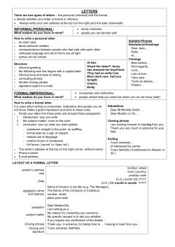


© Copyright 2026