
DEEP-CARVING : Discovering Visual Attributes by Carving Deep
DEEP-CARVING : Discovering Visual Attributes by Carving Deep Neural Nets
Sukrit Shankar† ,
Vikas K. Garg∗ and Roberto Cipolla†
†
∗
Machine Intelligence Lab (MIL), Cambridge University
Computer Science & Artificial Intelligence Lab (CSAIL), MIT
[email protected], [email protected], [email protected]
Abstract
1. Introduction
Owing to an exponential increase in the number of images on the web, most image search engines, such as
Google, have started resorting to clustering in order to
present the search results. In particular, they now categorize the images based on common and key attributes. On
receiving a query about tall buildings, for instance, Google
image search finds thousands of images it thinks contain tall
buildings, and then clusters them together into some key attributes such as night, looking-up. Analysing the images
in these clusters, we observe that the categorization is generally based more on the text information associated with
the images than the visual cues. Therefore, the attributes
that are missing in the text are rarely inferred in the images. Thus, it is difficult for the engine to determine which
buildings in the cluster of tall buildings at night are curved,
glassy, stony. Hence, the visual cues need to be leveraged
for enhancing the search results.
Discovering Visual Attributes under a Practical Scenario - Consider a practical system that can predict
attribute-specific information within images using visual
cues. For simplicity, suppose that we have only 3 attributes
of mountains under consideration, viz. wide-span, hazy and
with-reflections. If we search for hazy mountains, it is likely
that we get most mountains that seem hazy (with the increased accuracy of search engines), but some of them will
also have wide-span, some will exhibit reflections, some
will portray both wide-span and reflections, and some neither; however, typically, such information will not be found
in the text and thus remain unknown. We can then search
for wide-span mountains to get the visual cues (e.g., how
a wide-span mountain looks like), but the resulting images
might again contain varying and unknown degrees of haziness and reflections. Thus, the following problem abstraction arises naturally while designing a practical system for
visual attribute prediction:
Each of the M given attributes corresponds to a class.
Every training image in the class m ∈ {1, . . . , M } comes
with only one label that indicates the presence of the mth
attribute. The task is to discover all the attributes present in
Most of the approaches for discovering visual attributes in
images demand significant supervision, which is cumbersome
to obtain. In this paper, we aim to discover visual attributes in
a weakly supervised setting that is commonly encountered with
contemporary image search engines.
For instance, given a noun (say forest) and its associated
attributes (say dense, sunlit, autumn), search engines can now
generate many valid images for any attribute-noun pair (dense
forests, autumn forests, etc). However, images for an attributenoun pair do not contain any information about other attributes (like which forests in the autumn are dense too). Thus,
a weakly supervised scenario occurs: each of the M attributes
corresponds to a class such that a training image in class
m ∈ {1, . . . , M } contains a single label that indicates the presence of the mth attribute only. The task is to discover all the
attributes present in a test image.
Deep Convolutional Neural Networks (CNNs) [20] have enjoyed remarkable success in vision applications recently. However, in a weakly supervised scenario, widely used CNN training procedures do not learn a robust model for predicting multiple attribute labels simultaneously. The primary reason is
that the attributes highly co-occur within the training data, and
unlike objects, do not generally exist as well-defined spatial
boundaries within the image. To ameliorate this limitation, we
propose Deep-Carving, a novel training procedure with CNNs,
that helps the net efficiently carve itself for the task of multiple attribute prediction. During training, the responses of the
feature maps are exploited in an ingenious way to provide the
net with multiple pseudo-labels (for training images) for subsequent iterations. The process is repeated periodically after
a fixed number of iterations, and enables the net carve itself
iteratively for efficiently disentangling features.
Additionally, we contribute a noun-adjective pairing inspired Natural Scenes Attributes Dataset to the research community, CAMIT - NSAD, containing a number of co-occurring
attributes within a noun category. We describe, in detail,
salient aspects of this dataset. Our experiments on CAMITNSAD and the SUN Attributes Dataset [29], with weak supervision, clearly demonstrate that the Deep-Carved CNNs consistently achieve considerable improvement in the precision of
attribute prediction over popular baseline methods.
1
TRAINING
Instance
Instance
Label
Unsupervised
Label
Instance
Label
Instance
Label
Instance
Instance
Instance
Label
Label
Semi-supervised
Instance
Label
Instance
Label
Label
Instance
Label
Label
Instance
Label
Label
Multi-label
Label
Instance
Label
Multi-instance
Label
Instance
Label
Label
Label
Instance
Supervised
TESTING
Instance
Label
Label
Partial-label
Label
Noisy-label
Label
Label
OURS
Label
Label
Label
Instance
Label
Instance
Label
Instance
Label
Label
Instance
Label
Label
Figure 1. Understanding our Problem Setting for Attribute Prediction: A grey shaded box indicates unavailability. A green outlined box indicates
that the label is correct. From Left to Right: Supervised - Every instance has the correct label available. Unsupervised - No instance is labelled.
Semi-Supervised - Some instances have correct labels available, while some are not labelled. Multi-label - An instance has all correct labels available.
Multi-instance - Multiple instances together, not individually, have a correct label available. Partial-label - An instance has many labels available, out of
which only one can be correct. Noisy-label - An instance has multiple labels available, out of which more than one are possibly correct. Our Problem
Setting - An instance can have multiple correct labels, but only a single correct label is available. Also, no negative labels for instances or vice-versa are
available. In all cases, the test scenario shows the number of correct labels one needs to predict for a given instance. Figure is best viewed in color.
a test image using this weakly supervised training.
One might argue that instead of having weak supervision, why not search images with multiple attributes under consideration? Doing a joint search over attributes in
the query would lead to an exponential increase in the ambiguity. One might pose another question: why not train
exhaustively for each attribute with Amazon Mechanical Turk? Unlike object categories, training for a number
of attributes can be prohibitive.1 .
Image datasets for style recognition in scenes [19],
object-centric recognition (ImageNet [10]) and scenecentric recognition (MIT Places [45]) may not provide all
the positive correct labels for training instances. Nonetheless, researchers benefit from having to deal with a little mutual overlap across classes in the training set, and requiring
to estimate a limited number of (correct) labels in test data.
However, such luxuries do not always extend to the task of
attribute prediction, and thus, the weakly supervised setting
(as mentioned above in the problem abstraction) is more
challenging for predicting attributes than objects/scenes.
2. Related Work
We now briefly outline the related works on attributes
in computer vision, and label prediction in machine learning. Most existing approaches for discovering visual attributes/labels either require significant supervision or have
1 To see this, note that each attribute is connected to a noun, and with
at least 5000 popular noun and adjective synsets each (as per the WordNet [12]), there will be around 25 million attribute-noun combinations.
Typically 10% of such attribute-noun pairs, or roughly 2.5 million, can be
deemed to be valid (as per the ImageNet Attribute dataset [32] statistics).
Training about 400 images per valid attribute-noun pair will require on
the order of 1 billion positive labels, which is cumbersome to obtain. Alternatively, since a same attribute can exist for many different nouns, one
might not have separate classes for noun-attribute pairs; instead one might
have an attribute class containing multiple noun categories. Although this
decreases the amount of training required, it also increases per-class ambiguity, and usually affects the robustness of the model.
less co-occurrence within the training data, and thus do not
conform to our problem setting (see Fig 1 for a succinct
overview of related problems). We refer the readers to peruse these works for a holistic overview of the field.
Binary Attributes for Better Classification - In the
computer vision community, attribute learning has been
conventionally used to provide cues for object and face
recognition [21, 22], zero-shot transfer [22, 32], and part localization [11, 41]. There have also been attempts to make
learning and classification on categorical attributes robust:
for instance, [30] strives to make the binary attributes more
discriminative on a class basis. However, all these methods
require complete attribute labelling for the training images.
Relative Attributes - Another direction of work [28,34]
considers ranking image classes or instances according to
the attributes, and training a feature space such that the
maximum number of pairwise rank constraints are satisfied.
Again, such methods require complete supervision, and
thus cannot be applied to our problem. Likewise for the various multi-label ranking methods such as [4,6,14,16,18,36]
considered in the machine learning literature, which propose different types of feature models for efficient rank
learning or label prediction, and the associated ensemble
methods for multi-label classification such as [31, 40]. Authors in [25] try to rank attributes in images in a completely
unsupervised manner. Their approach behaves rather ambiguously while predicting multiple attributes, and suffers
from issues of scalability as well. To counter this problem, [33] considers a weakly-supervised scenario and estimates the ranking of images based on the attributes. This
approach yields promising results, however, it requires semantic response variables for some images and thus does
not apply to our setting.
Predicting Attributes using Textual Information Some works like [3,42] aim to estimate the attributes in images, but rely on the availability of text information, which
does not hold for our setting. Similarly, [32] tries to pre-
L5
L6
L7
L8
L4
L2
Input Image
L1
DEEP-CARVING
Sigmoid Cross Entropy Loss
Input Image
L1
L5
L6
L7
L8
L3
Sigmoid Cross Entropy Loss
L4
L3
L2
RETRAIN
Analyse the convolutional layers to provide pseudo labels to the multi label loss layer
Figure 2. Illustration of Deep-Carving: Deep-carving is a novel training procedure with deep CNNs. During training, the responses of the feature maps
are exploited in an ingenious way to provide the net with multiple pseudo-labels (for training images) for subsequent iterations. The process is repeated
periodically after a fixed number of iterations once the net has learnt reasonably disentangled feature map representations. This eventually enables the net
carve itself iteratively for efficiently predicting multiple attribute labels. Yellow, Red, Green coloured feature maps indicate their firing for three attributes in
consideration, while blue coloured feature maps indicate that they fire for all three attributes. After deep-carving, the feature maps are better disentangled
(evaluated through multi-label classification results). The last layer L8 is shown in a different color, since it always contains the number of attribute classes
as its number of outputs, based on which probabilities are calculated. Figure is best viewed in color.
dict attributes in the ImageNet dataset [10], but expects all
attribute labels to be present in the training data.
Predicting Attributes under Weak Supervision - The
main idea behind [15,23] is to use an Entropy Minimization
method to create low-density separation between the features obtained from deep stacked auto-encoders. Their work
can be deemed to be nearest to our proposed approach; however, we do not deal with unlabelled data, and tend to follow
a more comprehensive approach for attribute prediction. [9]
proposes a weakly supervised graph learning method for
visual ranking of attributes, but the graph formulation is
heavily dependent on the attribute co-occurrence statistics,
which can often be inconsistent in practical scenarios. Researchers in [43] attempt to leverage weak attributes in images for better image categorization, but expect all weak
attributes in the training data to be labelled. Authors in [7]
solve the partial labelling problem, where a consideration
set of labels is provided for a training image, out of which
only one is correct. However, as depicted in Fig 1, each
training image in our problem setting can have more than
one correct (but unlabelled) attribute.
Label Prediction with Deep CNNs - Deep CNNs have
recently enjoyed remarkable success for predicting object
[10] and scene labels [45]. Such works contain only one
correct label for each training instance, and predict multiple
labels for the test images, as in our problem setting (Fig 1).
However, as mentioned before, the same problem setting
when applied for attribute prediction is much more challenging, since attributes generally co-occur in abundance
within the training instances and cannot be always separated by well-defined spatial boundaries. Thus, deep CNNs
clearly require enhancements, more so when false positives
also need to be minimized.
To the best of our knowledge, we are the first to target
such a weakly supervised problem scenario for multiple attribute prediction. We now summarize the key contributions of this paper:
1. We emphasize the weakly supervised scenario commonly
encountered with image search engines, with an aim to discover multiple visual attributes in test images (see Fig 1).
2. We introduce a noun-adjective pairing inspired Natural
Scenes Attributes Dataset (CAMIT-NSAD) having a total of
22 pairs, with each noun category containing a number of cooccurring attributes. In terms of the number of images, the
dataset is about three times bigger than the SUN Attributes
dataset [29].
3. We introduce Deep-Carving, a novel training procedure
with CNNs, that enables the net efficiently carve itself for
the task of multiple attribute prediction.
3. Approach
Recall the problem definition from Section 1. Let
A = {a1 , . . . , aM } be the set of M attributes under consideration. We have a weakly supervised training set, S =
{(x1 , y1 ), . . . , (xN , yN )} of N images x1 , . . . , xN ∈ X
having labels y1 , . . . , yN ∈ A respectively. Equivalently,
segregating the training images based on their label, we
obtain M sets S m = X m × am , where X m = {x ∈
X|(x, am ) ∈ S} denotes the set of Nm = |X m | images
each having the (single) positive training label am , m ∈
{1, . . . , M }. For a test image xt , the task is to predict
yt ⊆ A, i.e. all the attributes present in xt .
Motivation for Using Deep CNNs to Predict Attributes: Deep CNNs have recently shown state-of-the-art
performance on the tasks of predicting key facial points and
facial expressions [1, 38]. Although CNNs have been used
extensively for object recognition [20], researchers [29]
have conventionally used low-level features for attribute
prediction in scenes. We compared attribute prediction performances on the SUN Attributes Dataset (with weak supervision) using the state-of-the-art ensemble of low-level
features proposed in [29] and the deep CNN architecture
proposed in [20], and found that under a weakly supervised
scenario, deep CNNs outperformed the low-level features
L3
L4
L5
L6
L7
L8
Conv + Pool
Conv
Conv
Conv + Pool
Full Connect
Full Connect
Full Connect
(Other variants possible)
L2
Softmax Loss Layer
L1
Conv + Pool
Input Image
for attribute prediction in scenic images (details provided in
Section 4).
Some researchers have also used Deep Belief Nets
(DBNs) [39] for expression (attribute) recognition in faces.
However, CNNs are generally more attractive since being
translation-invariant, unlike DBNs, they can be used with
unconstrained datasets. Though convolutional forms of
DBNs exist [24], they have not shown much promise over
deep CNNs for most of the recognition tasks. Consequently,
deep CNNs are an obvious choice to consider for the task
of attribute prediction.
Figure 3. Block Illustration of AlexNet [20]: The deep convolutional
neural net architecture has eight layers (L1 − L8) after the input. The last
fully connected layer is conventionally followed by a softmax loss layer,
but can also be replaced by the likes of Sigmoid Cross Entropy Loss Layer
[17]. We use this as the base CNN architecture for all our experiments.
analysed in a novel way after every fixed number of iterations during training, and the net eventually carves itself for
predicting multiple attribute labels more robustly.
We call this approach deep-carving and argue that it is
inherently different from the fine-tuning and dropout procedures. Dropout methods like [37] drop parts of the net
randomly (without analysing the current training state) to
avoid overfitting, while adaptive dropout procedures like [2]
drop parts by analysing the state of the net during training
iterations. Fine-tuning procedures [19] take a pre-trained
net and mainly learn the last layer parameters (while only
perturbing the parameters of the other layers) on their training set for a given loss. We instead analyse the net during
training to provide a set of new (pseudo) outputs for missing
labels in subsequent iterations, which helps the net to carve
out attribute-specific feature maps.
Training the Net using Deep-carving: We consider
AlexNet (Fig 3) as our base architecture. With the softmax
loss layer, the training of the AlexNet is typically accomplished by minimizing the following cost or error function
(negative log-likelihood):
Ls = −
The CNN Architecture: Inspired by its huge success [13, 17, 44], we use AlexNet [20] as our base deep
CNN architecture (Fig 3) for all our purposes. The fullyconnected layers have 4096 neurons each. Max-pooling is
done to facilitate translation-invariance. For the fully connected layers, a drop-out [37] probability of 0.5 is used to
avoid overfitting. The final fully connected layer takes the
outputs of L7 as its input, produces M (equal to the number
of classes) outputs through a fully connected architecture,
then passes these outputs through a softmax function, and
finally applies the negative log likelihood loss. With softmax loss layer, each input image is expected to have only
one label. When softmax loss layer is replaced by a sigmoid cross-entropy loss layer, the outputs of L8 are applied
to a sigmoid function to produce predicted probabilities, using which cross-entropy loss is compute. Here each input
can have multiple label probabilities. We refer the reader
to [20] for details on the kernel and filter sizes of the layers.
Motivation behind Deep-Carving: From our problem
description, it is clear that the attribute-specific information
needs to be present in a decently segregated form in the output feature vectors. We avail the fact that deep CNNs, even
under a weakly supervised scenario, learn a set of reasonably disentangled feature maps during initial stages of training; however, they start to get befuddled (evident from unstable convergence trends) in later stages of training due to
lack of all correct labels. We thus devise a method to provide the net with pseudo-labels for training images, once
the net has initially learned reasonable feature map representations. For this, the responses of the feature maps are
N
1 X
log(ˆ
pr,yr )
N r=1
(1)
where the probability pˆr,yr , r ∈ {1, . . . , N }, is obtained by
applying the softmax function to the M outputs of layer L8.
Letting lr,m denote the mth output for xr , we have
pˆr,m = P
elr,m
,
lr,m0
m0 e
m, m0 ∈ {1, . . . , M }.
(2)
Note here that for the softmax loss, the labels yr ∈ A
are encoded in the corresponding range {0, . . . , M − 1} for
computational purposes. In case one applies the sigmoid
cross entropy loss, each image r is expected to be annotated with a vector of label probabilities pr , having length
M . For our weakly supervised case, the vector pr is initialized with a very low value of 0.05 for all images, with
pm
r = 0.95 ∀ r ∈ X m . With sigmoid cross-entropy loss,
the network is trained by minimizing the following loss objective:
Le = −
N
1 X
[pr log(p
ˆr ) + (1 − pr ) log(1 − p
ˆr )]
N r=1
(3)
where the probability vector pˆr is obtained by applying the
sigmoid function to each of the M outputs of layer L8.
To learn a deep-carved net, we follow the sigmoid crossentropy loss since it can take into account the probabilities
of multiple labels. For a deep-carving iteration c, the following loss is minimized:
Lce = −
N
1 X c
[pr log(p
ˆr ) + (1 − pcr ) log(1 − p
ˆr )]
N r=1
(4)
Algorithm 1: Generating Pseudo-labels for Deep-carving
for all feature maps f in convolutional layers do
for all attribute classes am ∈ A do
for all images r ∈ Xm do
Calculate wrm , average spatial response at f for r
end
Average wm over r to produce tm
Assign hm
f = tm .
end
end
hf is the histogram of average responses at feature map f from all
training images for M attribute classes.
for all images r in the training set S do
for all feature maps f in convolutional layers do
Calculate vfr , average spatial response of r at f
for all attribute classes am ∈ A do
if am == yr then
zrf,m = 0.95
else
r
m
if γhm
f ≤ vf ≤ hf then
zrf,m = vfr /hm
f
else
zrf,m = 0.05
end
end
end
Average z m
r over all feature maps f to obtain br of
length M .
end
Form the pseudo labels as pc,m
= bm
r
r . Here c stands for the
deep-carving iteration.
labels for all subsequent iterations till the successive deepcarving iteration. This helps the net to slowly carve itself for
efficiently predicting the attribute labels. For all our experiments, we set γ = 0.7; this is empirically selected and indicates that pseudo-labels are only assigned when the chances
of co-occurrence of the missing attributes are significantly
high.
For a given deep-carving iteration c, the pseudo-label
probabilities generated by Algorithm 1 are different from
the output probabilities that the net would have generated.
This is because the latter is affected by the fully connected
layer parameters that are learnt based on weakly supervised
label set, unlike the former.
Prediction using a Learned Model: Given a test image, the number of positive labels (say K) is known from
the ground-truth. Thus, K denotes the number of correct
attributes that need to be predicted for the respective test
image. Let T contain the positive labels for the test image. Given the sorted (in descending order) probabilities
for the test image from the prediction model, we pick top
K predictions. Let the set P contain these predicted labels. Both T and P have cardinality K. We then calculate
the number of true and false positives using T and P , and
use precision as our performance metric. Note that this is
a stricter performance metric compared to the conventional
top-K accuracy, where the presence of at least one correct
label out of the top K predictions suffices. We thus believe
that our chosen performance metric helps better gauge the
prediction models.
end
4. Results and Discussion
where the probability vector pcr is a vector of pseudolabel probabilities (we shall interchangeably refer them as
pseudo-labels) computed by Algorithm 1.
The method outlined in Algorithm 1 was optimized on
the GPU for computational efficiency; however, we have
presented the algorithmic steps in a much simpler way to
enhance didactic clarity. Note that during the generation of
pseudo-labels, we do not change the initially available labels in the training set S. The process of predicting pseudolabels is repeated for each deep-carving iteration c, which is
chosen periodically after every 5 epochs, once we have already trained for around 60 epochs. Thus, we are delivering
the pseudo-labels to the net after some fixed intervals, and
that too after the net has initially learnt reasonably disentangled feature maps.
We only consider the feature maps of convolutional layers for Algorithm 1. Ideally, the fully connected layers
learn their parameters taking the inputs from the convolutional layers and minimizing the cross-entropy loss with
original (weakly supervised) labels. After a deep-carving iteration, the net considers the pseudo-labels as its new set of
We now present the results of our experiments with deepcarved CNNs and several baselines on two natural scenes
attribute datasets. We also provide details on and motivation
behind the new attribute database we introduce in this paper.
Types of Visual Attributes: In the computer vision
literature, many different categories for visual attributes
have been considered, with the most common being: (a)
Shape (round, rectangular, etc.), (b) Texture (wet, vegetation, shiny, etc.), (c) Proper Adjectives (cute, dense, chubby,
etc.), (d) Nouns that cannot be regarded as objects or parts
(resorts, sunset, etc.), (e) Colour (red, green, grey), (f)
Nouns that denote objects or specific parts of an object
(oceans, flowers, clouds, etc.), and (g) Verbs that define a
human body pose or activity (hiking, farming). Most of
these attribute categories are covered in the SUN Attributes
Dataset [29]. In this paper, we only consider attributes that
fall into the categories (a),(b),(c), or (d). We make this
choice to ensure that we do not try to solve a problem under the paradigm of attribute prediction that can be solved
more efficiently using existing approaches in computer vision. For instance, color attributes can generally be discovered by color histograms, human activities (functions)
are amenable to pose or activity recognition methods, and
nouns that refer to objects can be predicted by using largescale object recognition datasets (like ImageNet).
SUN Attributes Dataset [29]: The SUN Attributes
dataset (SAD) has 102 attributes and contains a total of
14,340 images depicting natural scenes. Each image has
annotations to indicate the degree of presence of all 102 attributes. Each positive label in SAD is associated with a
confidence value. Confidence values of 0.66 and 1 suggest
strong presence of an attribute, while a confidence value of
0.33 indicates an ambiguous presence. Given the types of
attributes that we ought to consider in this paper, we select
42 suitable attributes (listed in Fig 4) out of 102 choices.
To use SAD for our weakly supervised scenario, for each
attribute class, we algorithmically choose images from SAD
that have a strong presence of that attribute. We choose at
least 250 images for each attribute class, while ensuring that
the number of overlapping images across attribute classes is
minimal. We thus obtain 22,084 images for training, 3056
images for validation and 5618 images for testing. The
training set contains at least 150 images for each attribute
class. The training and validation images chosen for a particular attribute class are all given a single label that indicates the presence of the respective attribute. For each test
image, the ground truth comprises of possibly multiple positive labels, thereby indicating strong presence of multiple
attributes.
Note that we choose the images from SAD with a slight
overlap of images across attribute classes, without introducing any fundamental change to our problem setting, to aptly
capture the common real world scenario: in image search
engines, there is a small possibility of obtaining same images for different attribute-related queries. For instance, we
expect some overlap in the results retrieved from queries for
sunset beaches and resort beaches, since some images in
the two collections might have both beaches and resorts in
their textual information. We preferred SAD over other attribute datasets such as ImageNet [32] and OSR [27] since
these contain few attributes of our interest. Also, we do
not consider style recognition datasets like Aesthetic Visual
Analysis [26] in this paper, since they mainly contain photographic attributes instead of general scene attributes. However, our algorithm is generic enough to be applied to style
recognition datasets as well.
Natural Scenes Attributes Dataset: SAD contains attributes for natural scenes in general. However, it does not
segregate attributes in relation to a specific noun. In practice, people typically search for an attribute-noun pair rather
than an attribute. For instance, it is more common to search
for beautiful valleys instead of just beautiful. Therefore,
we introduce the Cambridge-MIT Natural Scenes Attributes
Dataset (CAMIT-NSAD) that contains attribute-noun pairs.
For a given noun, the attributes co-occur significantly in
CAMIT-NSAD. Moreover, different nouns can co-occur in
a scene occasionally (dark skyscapes with sunset beaches,
etc.). Some of the most popular attributes and nouns on
500px / Flickr have been selected for CAMIT-NSAD (refer
to Fig 4 for a complete overview).
CAMIT-NSAD contains 46,008 training images, with at
least 500 images for each attribute-noun pair. The validation set and the test set contain 2104 and 2967 images
respectively. All images in CAMIT-NSAD were collected
from 500px, Flickr and Google Search engine, and manually cleaned for every attribute-noun pair. For ground truth,
the test set images were annotated for the presence/absence
of attribute-noun pairs. CAMIT-NSAD, as a natural scenes
attributes dataset, is quite different to SAD. While the nounattribute pairs make object and attribute detection more
specifically related, there is generally lesser co-occurrence
across classes, but much more within a noun class. Although this helps to make the prediction model robust, discovering attribute-noun pairs still remains challenging with
deep CNNs.
All images in SAD and CAMIT-NSAD are 256 × 256
RGB. For a test image, the number of positive labels (say
K) was known from the ground-truth, using which precision was calculated according to Section 3 for gauging the
performance.
All our deep learning related experiments were conducted on NVIDIA TITAN GPUs using Caffe Library [17].
We configured Caffe to use Stochastic Gradient Descent
(SGD), and stopped the training after a maximum of 500
epochs. Manual tuning procedures with SGD were carried
out using the heuristics mentioned in [17] and [5].
Low-level Features vs Deep CNNs for Attribute Prediction on SAD: We compared attribute prediction using
deep CNNs, on SAD (with weak supervision), with the
state-of-the-art low-level feature ensemble of [29], which
combines color histograms, histogram of oriented gradients [8], self-similarity, and gist descriptors [27]. We tried
two cases with combined low-level features. First, when
the features were simply concatenated; and second, when
the features were individually normalized before concatenation. Note that unlike [29], we did not learn separate
classifiers for each low-level feature, in order to draw a fair
comparison with deep net features. As shown in Fig 5,
AlexNet performed better than the low-level features. Normalized low-level feature combination significantly outperformed the simply concatenated one2 .
Baselines: We consider three major baselines for comparing our deep-carved nets. First, we choose Alexnet
with softmax loss layer because of its immense popular2 Some researchers [19] have tried to concatenate the low-level features
and deep net features to improve results for the recognition of styles in
scenes. However, we do not follow this approach, since the main aim of our
work is to show that deep-carving can help improve the conventional deep
learning results on attribute recognition in a weakly supervised scenario.
ve
g
sh eta
ru tio
fo bb n
lia er
le ge y
a
sh ves
i
co ngl
n c es
re
t
pa e
pe
w r
oo
vi dy
ny
ru l
b
cl ber
ot
sa h
n
ro d
ck
di
rt
m
a
gl rble
a
w ss
av
r u es
n
st nin
ill g
sn wa wa
o te te
na w r r
t
di ura
re l
el ct ligh
e su t
ag ctric n
e
gl d
o
m ssy
a
m tte
o
dr ist
y
di
rt
ru y
s
w ty
ar
co m
ld
na
t
m ura
a l
op n m
e a
fa n a de
r h re
ru o r a
g iz
sy ged on
m
cl me e
ut t n
sc ter ric e
a e
so ry d
ot
hi
ng
SUN ATTRIBUTES DATASET (our selection)
m
sc
al
et
Forests
fro
smzen
oo
th
ta
l
l
u
da
de r k
ns
e
y
on
st
Buildings
Beaches
fo
gg
re y
fl
sn ect
o io
su w y n s
n
v e s et
g
w eta
id tio
es n
pa
n
au
t
da m
r n
sn k
o
su wy
nl
it
cu
r
gl ved
a
lig ss
ht
ed
da
rk
re
s
su orts
ns
et
NATURAL SCENES ATTRIBUTES DATASET (OURS)
Mountains
Skyscapes
Waterfalls
Figure 4. Attribute Choices and Co-occurrence: The figure shows the attributes considered for SAD and CAMIT-NSAD. SAD contains 42 attributes
and CAMIT-NSAD contains 18 attributes and 22 attribute-noun pairs. Note that the images in SAD contain attributes like marble, glass, sand, cloth, etc.
as textures, instead of object-like things. For each dataset, attribute co-occurrence matrices are shown. Each matrix is square, with rows and columns
corresponding to the respective attributes in the order in which they are written. Thus, for SAD, matrix is of size 42 × 42, and so on. Let the set of
images that contain the attribute represented by a given row be C. Then, each column entry in that row is the number of images from C that contain the
attribute represented by that column divided by the total number of images in C. Thus, diagonal elements are always one, and the co-occurrence statistics is
contained in off-diagonal elements. A yellowish pixel indicates greater co-occurrence than a green one. CAMIT-NSAD generally shows high co-occurrence
within a noun class as compared to SAD. However, models generally benefit from less co-occurrence of nouns. For some mutually exclusive attributes such
as frozen and smooth for waterfalls, there is no co-occurrence and thus the off-diagonal elements are all green. The co-occurrence statistics are known for
the test data sets, and not training, since complete annotations are available only for the test images. Since test set is taken from the same pool of images as
that of the training set, co-occurrence statistics presented for test can be deemed to be roughly the same for training data as well. The matrices have been
scaled appropriately for better visibility. Figure is best viewed in color.
80
SAD
60
40
20
ne
co
ld
na
tu
an ral
m
o p ade
en
fa are
rh
a
ug oriz
ge
on
d
sy s e
m
m
et
r
cl ical
ut
te
re
d
sc
a
s o ry
ot
hi
ng
c
m
l
pa
pe
r
oo
dy
vi
ny
l
ru
bb
er
cl
ot
h
sa
nd
ro
ck
di
r
m t
ar
bl
e
gl
as
s
w
ru
nn ave
s
in
g
w
st ate
ill
r
w
at
er
na s n
o
tu
ra w
ll
di ight
re
ct
su
el n
ec
t ri
c
ag
ed
gl
os
sy
m
at
te
m
oi
st
dr
y
di
rty
ru
st
y
w
ar
m
a
et
m
w
ve
ge
ta
sh tion
ru
bb
er
y
fo
lia
g
le e
av
e
sh s
in
gl
c o es
nc
re
te
Precision
Figure 5. Comparison of Attribute Prediction Results: Left Table - Average precision on the SAD (weakly supervised) with combined-low-level
features, normalized combined-low-level features and AlexNet (Fig 3) with Softmax and Sigmoid Cross Entropy Loss Layers. AlexNet outperforms the
low-level feature methods. Right Table - Average precision on CAMIT-NSAD for AlexNet with Softmax and Sigmoid Cross Entropy Layers. In both cases,
fine-tuned AlexNet over the MIT Places dataset does not perform well, while deep-carved nets exhibit significant improvement over the AlexNet baselines.
r
60
40
s
Beaches
o
st
ny
ta
au l l
tu
n
da
rk
sn
ow
y
su
nl
it
fo
r e g gy
fle
ct
io
ns
sn
ow
su y
ve nse
ge t
ta
w tion
id
es
pa
n
da
rk
de
ns
e
fro
ze
sm n
oo
th
re
so
rts
un
se
cu t
rv
ed
gl
as
s
li g
ht
ed
rk
20
da
Precision
CAMIT-NSAD
80
m
Buildings
Forests
Mountains
Sky
Waterfall
Figure 6. Attribute-Wise Results with our Deep-Carved CNNs: The precision of predicting attributes / attribute-noun pairs with deep-carved nets for
SAD and CAMIT-NSAD is bar-plotted. It can be seen that the attributes that are less abstract and have lesser chances to co-occur with other attributes in an
image are easily predicted in general. Attributes such as symmetrical which involve structural relations are difficult to predict, unless they are paired with
a specific noun category (mountains-reflections). Attributes such as dark beaches can be sometimes ambiguous for the net, since evening and night beach
images are both considered as dark; however, their color tones are different.
ity and success in vision recognition tasks. Second, we
choose AlexNet architecture with a sigmoid cross-entropy
loss layer, since it better mimics the multi-label prediction
scenario as compared to a softmax loss layer. Third, owing to the recent success of MIT Places dataset for scene
recognition, we fine-tune their pre-trained model with our
training data using the softmax layer loss. Their pre-trained
models follow the AlexNet architecture, and during finetuning, we mainly learn the L8 layer parameters while allowing the parameters of other layers only to get perturbed3 .
Comparison with Deep-carved CNNs: Fig 5 shows
3 This is done in Caffe by setting the blobs lr parameter to 10 for
layer L8, while keeping it 1 for the other layers. The number of outputs in
L8 are also changed to the number of attribute classes M .
shingles, glassy,
natural light,
direct sun,
symmetrical
marble
metal, vinyl,
glassy,
electric, glossy,
matte, rusty,
man made,
cluttered cloth
beaches
(sunset),
mountains
(vegetation)
buildings
(lighted, tall,
stone, curved)
woody,
electric,
man made
woody,
cloth,
cluttered
paper
buildings
(stone, tall)
mountains
(reflections,
snowy,
vegetation,
widespan)
skyscapes
(dense)
leaves,
running water,
natural light
metal, woody,
electric, aged,
glossy, dirty
leaves,
running water,
natural light,
foliage
metal, woody,
electric, glossy
skyscapes
(dark,
dense)
waterfalls
(smooth)
Figure 7. Attribute Predictions with our Deep-Carved CNNs: The correctly predicted attributes (true positives) shown in green, and the wrongly
predicted ones (false positives) shown in red for various instances in SAD (top row) and CAMIT-NSAD (bottom row) with our deep-carved CNNs. The
attributes that are abstract in nature or heavily co-occur with other attributes, are generally predicted with lesser accuracy. Figure is best viewed in color.
Figure 8. Visualization of the Filters for the first Convolutional Layer of: From Left to Right - Deep-carved AlexNet for SAD and CAMIT-NSAD,
fine-tuned AlexNet over Places205 Model (MIT Places Dataset) for SAD and CAMIT-NSAD. There are 96 filters of sizes 11 × 11 with 3 channels for each
learnt model, and are shown here on a 10 × 10 grid. There is hardly any difference between the last two filter sets, since during fine-tuning, the last full
connected layer parameters were only learnt from scratch (random initialization), while the parameters of all the other layers were only perturbed. This is
the standard outline for fine-tuning pre-trained Caffe Models as listed out in [17]. Figure is best viewed in color.
a comparison of the baselines with our deep-carved nets
on SAD and CAMIT-NSAD, while Fig 6 shows attributewise performance of our deep-carved CNNs. It is clear that
deep-carved CNNs significantly outperform the baselines.
Note that the results with fine-tuning of Places models for
our datasets show drastically decreased performance. Although the MIT Places dataset (we consider the 205 categories variant) contain similar images to that of SAD and
CAMIT-NSAD, the fine-tuned net mostly outputs low probabilities for the correct attributes, as it gets confused having
been apriori trained on a lot of scene categories. The results might get better if one fine-tunes with more number of
layers instead of just L8. Fig 8 helps to understand this better. It can be seen that the fine-tuned models generally contain very crisp object-specific (edge-like) filters in their first
convolutional layer, and seem less oriented towards learning attribute-specific filters (color patterns, mixed textures).
On the other hand, deep-carved nets for CAMIT-NSAD
learn some object-specific and some attribute-specific filters. This is understandable since the classes in training set
of CAMIT-NSAD contain noun-attribute pairs. The deepcarved nets on SAD learn very less of object-specific filters and more of color patterns, as the training classes are
not particular to any noun category, rather contain multiple
noun categories. One might infer the merging color patterns to represent scene-specific features; however, our experiments on CAMIT-NSAD show that such patterns more
precisely encode attributes of well-categorized scenes. Al-
though inversion of CNN features [35] for different input
images might be more appropriate for analysing the filters
and feature map responses, the marked differences in the
filters of the first convolutional layer give a fair indication
of how the net might be getting biased.
Fig 7 shows examples of the attributes correctly / incorrectly detected for test images in SAD and CAMIT-NSAD.
When the co-occurring attributes are abstract and heavily
co-occur with other attributes within an image, the number
of false positives generally increases. Attribute-wise accuracy with deep-carved nets can be seen in Fig 6.
5. Conclusions and Future Work
We have targeted the weakly supervised scenario commonly encountered with image search engines, with an
aim to discover multiple visual attributes in images. We
have proposed a novel training procedure with CNNs called
Deep-Carving, that helps the net efficiently carve itself
for the task of multiple attribute prediction. We have
also introduced a noun-adjective pairing inspired natural scenes attributes dataset (CAMIT-NSAD), with each
noun category containing a number of co-occurring attributes. Our results show that deep-carving significantly
outperforms several popular baselines for our weakly supervised problem setting. CAMIT-NSAD and the pretrained deep-carved Caffe Models can be accessed from
http://mi.eng.cam.ac.uk/∼ss965/.
References
[1] Deep learning faces. https://code.google.com/p/
deep-learning-faces/. 3
[2] J. Ba and B. Frey. Adaptive dropout for training deep neural
networks. In Advances in Neural Information Processing
Systems, pages 3084–3092, 2013. 4
[3] T. L. Berg, A. C. Berg, and J. Shih. Automatic attribute discovery and characterization from noisy web data. In ECCV,
pages 663–676. Springer, 2010. 2
[4] T. Bernecker, H.-P. Kriegel, M. Renz, and A. Zuefle. Probabilistic ranking in uncertain vector spaces. In Database Systems for Advanced Applications, 2009. 2
[5] L. Bottou. Stochastic gradient descent tricks. In Neural Networks: Tricks of the Trade, pages 421–436. Springer, 2012.
6
[6] W. Chu and Z. Ghahramani. Gaussian processes for ordinal
regression. In JMLR, pages 1019–1041, 2005. 2
[7] T. Cour, B. Sapp, and B. Taskar. Learning from partial labels.
JMLR, 12:1501–1536, 2011. 3
[8] N. Dalal and B. Triggs. Histograms of oriented gradients for
human detection. In Computer Vision and Pattern Recognition, 2005. CVPR 2005. IEEE Computer Society Conference
on, volume 1, pages 886–893. IEEE, 2005. 6
[9] C. Deng, R. Ji, W. Liu, D. Tao, and X. Gao. Visual reranking
through weakly supervised multi-graph learning. 3
[10] J. Deng, W. Dong, R. Socher, L.-J. Li, K. Li, and L. FeiFei. Imagenet: A large-scale hierarchical image database. In
CVPR, pages 248–255. IEEE, 2009. 2, 3
[11] A. Farhadi, I. Endres, D. Hoiem, and D. Forsyth. Describing
objects by their attributes. In CVPR, 2009. 2
[12] C. Fellbaum. WordNet. Wiley Online Library, 1998. 2
[13] R. Girshick, J. Donahue, T. Darrell, and J. Malik. Rich feature hierarchies for accurate object detection and semantic
segmentation. arXiv preprint arXiv:1311.2524, 2013. 4
[14] Y. Gong, Y. Jia, T. Leung, A. Toshev, and S. Ioffe. Deep
convolutional ranking for multilabel image annotation. arXiv
preprint arXiv:1312.4894, 2013. 2
[15] Y. Grandvalet, Y. Bengio, et al. Semi-supervised learning by
entropy minimization. In NIPS, volume 17, pages 529–536,
2004. 3
[16] J. Guiver and E. Snelson. Learning to rank with softrank and
gaussian processes. In ACM SIGIR, 2008. 2
[17] Y. Jia, E. Shelhamer, J. Donahue, S. Karayev, J. Long, R. Girshick, S. Guadarrama, and T. Darrell. Caffe: Convolutional
architecture for fast feature embedding. In Proceedings of
the ACM International Conference on Multimedia, pages
675–678. ACM, 2014. 4, 6, 8
[18] T. Joachims. Optimizing search engines using clickthrough
data. In ACM SIGKDD, 2002. 2
[19] S. Karayev, A. Hertzmann, H. Winnemoeller, A. Agarwala,
and T. Darrell. Recognizing image style. arXiv preprint
arXiv:1311.3715, 2013. 2, 4, 6
[20] A. Krizhevsky, I. Sutskever, and G. E. Hinton. Imagenet
classification with deep convolutional neural networks. In
NIPS, volume 1, page 4, 2012. 1, 3, 4
[21] N. Kumar, A. C. Berg, P. N. Belhumeur, and S. K. Nayar.
Attribute and simile classifiers for face verification. In ICCV,
2009. 2
[22] C. H. Lampert, H. Nickisch, and S. Harmeling. Learning to
detect unseen object classes by between-class attribute transfer. In CVPR, 2009. 2
[23] D.-H. Lee. Pseudo-label: The simple and efficient semisupervised learning method for deep neural networks. In
Workshop on Challenges in Representation Learning, ICML,
2013. 3
[24] H. Lee, R. Grosse, R. Ranganath, and A. Y. Ng. Convolutional deep belief networks for scalable unsupervised learning of hierarchical representations. In Proceedings of the
26th Annual International Conference on Machine Learning,
pages 609–616. ACM, 2009. 4
[25] S. Ma, S. Sclaroff, and N. Ikizler-Cinbis. Unsupervised
learning of discriminative relative visual attributes. In ECCV
Workshop on Parts and Attributes, 2012. 2
[26] N. Murray, L. Marchesotti, and F. Perronnin. Ava: A largescale database for aesthetic visual analysis. In Computer Vision and Pattern Recognition (CVPR), 2012 IEEE Conference on, pages 2408–2415. IEEE, 2012. 6
[27] A. Oliva and A. Torralba. Modeling the shape of the scene: A
holistic representation of the spatial envelope. International
journal of computer vision, 42(3):145–175, 2001. 6
[28] D. Parikh and K. Grauman. Relative attributes. In ICCV,
2011. 2
[29] G. Patterson and J. Hays. Sun attribute database: Discovering, annotating, and recognizing scene attributes. In CVPR,
pages 2751–2758. IEEE, 2012. 1, 3, 5, 6
[30] M. Rastegari, A. Farhadi, and D. Forsyth. Attribute discovery via predictable discriminative binary codes. In ECCV.
2012. 2
[31] L. Rokach, A. Schclar, and E. Itach. Ensemble methods for
multi-label classification. arXiv preprint arXiv:1307.1769,
2013. 2
[32] O. Russakovsky and L. Fei-Fei. Attribute learning in largescale datasets. In Trends and Topics in Computer Vision,
pages 1–14. Springer, 2012. 2, 6
[33] S. Shankar, J. Lasenby, and R. Cipolla. Semantic transform:
Weakly supervised semantic inference for relating visual attributes. In ICCV, pages 361–368. IEEE, 2013. 2
[34] A. Shrivastava, S. Singh, and A. Gupta. Constrained semisupervised learning using attributes and comparative attributes. In ECCV. 2012. 2
[35] K. Simonyan, A. Vedaldi, and A. Zisserman. Deep inside
convolutional networks: Visualising image classification
models and saliency maps. arXiv preprint arXiv:1312.6034,
2013. 8
[36] M. A. Soliman and I. F. Ilyas. Ranking with uncertain scores.
In ICDE, 2009. 2
[37] N. Srivastava, G. Hinton, A. Krizhevsky, I. Sutskever, and
R. Salakhutdinov. Dropout: A simple way to prevent neural
networks from overfitting. The Journal of Machine Learning
Research, 15(1):1929–1958, 2014. 4
[38] Y. Sun, X. Wang, and X. Tang. Deep convolutional network cascade for facial point detection. In Computer Vision
[39]
[40]
[41]
[42]
[43]
[44]
[45]
and Pattern Recognition (CVPR), 2013 IEEE Conference on,
pages 3476–3483. IEEE, 2013. 3
J. M. Susskind, G. E. Hinton, J. R. Movellan, and A. K.
Anderson. Generating facial expressions with deep belief
nets. Affective Computing, Emotion Modelling, Synthesis
and Recognition, pages 421–440, 2008. 4
G. Tsoumakas, I. Katakis, and L. Vlahavas. Random
k-labelsets for multilabel classification. Knowledge and
Data Engineering, IEEE Transactions on, 23(7):1079–1089,
2011. 2
G. Wang and D. Forsyth. Joint learning of visual attributes,
object classes and visual saliency. In ICCV, 2009. 2
S. Wang, J. Joo, Y. Wang, and S.-C. Zhu. Weakly supervised learning for attribute localization in outdoor scenes. In
CVPR, pages 3111–3118. IEEE, 2013. 2
F. X. Yu, R. Ji, M.-H. Tsai, G. Ye, and S.-F. Chang. Weak
attributes for large-scale image retrieval. In CVPR, pages
2949–2956. IEEE, 2012. 3
M. D. Zeiler and R. Fergus. Visualizing and understanding
convolutional networks. In Computer Vision–ECCV 2014,
pages 818–833. Springer, 2014. 4
B. Zhou, A. Lapedriza, J. Xiao, A. Torralba, and A. Oliva.
Learning deep features for scene recognition using places
database. In Advances in Neural Information Processing Systems, pages 487–495, 2014. 2, 3


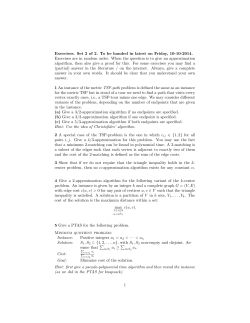
© Copyright 2026