
Drone-based traffic flow estimation and tracking using computer vision
UNIVERSITEIT•STELLENBOSCH•UNIVERSITY jou kennisvennoot • your knowledge partner Drone-based traffic flow estimation and tracking using computer vision by Andrew de Bruin: 16458826 Report submitted in partial fulfilment of the requirements of the module Project (E) 448 for the degree Baccalaureus in Engineering in the Department of Electrical and Electronic Engineering at the University of Stellenbosch Supervisor: Dr. Marthinus Johannes Booysen Department of Electrical & Electronic Engineering, Stellenbosch University. November 2014 DECLARATION i Declaration I, the undersigned, hereby declare that the work contained in this report is my own original work unless indicated otherwise. Signature Date ACKNOWLEDGEMENTS ii Acknowledgements To my Mother and Father for the continuous support and encouragement offered throughout my four years of study. To Dr. M.J. Booysen for the guidance, support and supervision he provided throughout the project. To Prof. T. Jones for organising the Parrot AR Drone, as well as for increasing my interest in control systems throughout my four years of study. To Prof. W.H. Steyn for his continuous guidance. To Dr. C.E. van Daalen for his assistance with control systems. To Dr. S.J. Andersen for his assistance with the traffic flow component. To Chané Bunning for helping with the design of the poster, as well as for the continuous support and encouragement she offered throughout the process. To my lab colleagues, Alexander Chiu and Jonathan Brown, for their motivation and good company. To Trintel and MTN for providing funding for the project. DEDICATION iii Dedication Science is a wonderful thing if one does not have to earn one’s living at it. Albert Einstein ABSTRACT iv Abstract Traffic flow estimation is a technique by which traffic engineers analyse the extent to which a particular road segment can accommodate traffic. Decisions regarding the need for road upgrades, the installation of speeding cameras and even general security upgrades are made based on these results. Since traffic cameras are usually installed throughout urban areas, exploiting this established infrastructure would allow for the seamless integration of an autonomous traffic flow estimation system. This can be achieved by designing a highly flexible and adaptive system, that would allow for the analysis of traffic footage from various input sources. The purpose of this project was to design and implement a system that allowed for autonomous traffic flow estimation using computer vision techniques. The system was required to compute traffic flow metrics and upload the information in real-time to an online dashboard. The Mixture of Gaussian (MoG) background subtraction technique was implemented throughout the project as the primary method of vehicle detection. Shadows were detected based on certain chromaticity characteristics, before being subsequently removed from the foreground mask. Relative vehicle velocities were computed based on optical flow tracking techniques. Results showed both the vehicle detection as well as the velocity computations to be around 95% accurate under ideal conditions, and around 80% under non-ideal illumination conditions. A particularly attractive alternative to the static pole-mounted traffic cameras, is the use of a fully autonomous aircraft. In this way, simple landing platforms could eventually replace expensive traffic cameras. This would allow for the analysis of traffic flow in more rural areas where the necessary infrastructure is often non-existent. The system designed to automate the aircraft flight control was implemented in the discrete-time domain using augmented difference equations. The method of least squares was used to obtain a model of the plant so that appropriate controllers could be designed. Ultimately, the Ziegler-Nichols tuning method was used to obtain the practical controller parameters. Results obtained during the testing procedure showed that the aircraft was able to land on the designated platform. The inclusion of the automated aircraft is intended to add additional functionality to the primary aim of this project. The system was designed in a modular fashion, with each submodule contributing additional functionality. The modules were then integrated and thoroughly tested to ensure optimal system performance. Results of the testing showed the system to be fully functional, and proved the concept of autonomous traffic flow estimation to be a viable option. UITTREKSEL v Uittreksel Meting van verkeersvloei, is ’n tegniek wat deur verkeersingenieurs gebruik word om die mate wat ’n spesifieke pad segment verkeer kan akkommodeer, te analiseer. Die resultate kan gebruik word vir besluitneming aangaande pad opgraderings, die installering van spoedkameras en selfs vir algemene sekuriteitsopgradering. Hierdie outonome verkeersvloeimetingstelsel, kan sonder veel moeite in ’n bestaande kamera infrastruktuur in veral beboude areas geïmplementeer word. Dit word vermag deur ’n hoogs buigbare en aanpasbare stelsel te ontwerp vir die analisering van verkeersopnames wat van verskeie intreebronne verkry word. Die doel van hierdie projek was om ’n stelsel te ontwerp en implementeer wat voorsiening maak vir outonome verkeersvloeimeting deur van rekenaarvisietegnieke gebruik te maak. ’n Vereiste was dat die stelsel verkeersvloei eienskappe visueel kan bereken, en die inligting dan op ’n aanlyn beheerpaneel in reële tyd oplaai. Die ‘Mixture of Gaussian’ (MoG) agtergrond-aftrekking tegniek, was regdeur die projek geïmplementeer as die primêre metode van voertuig opsporing. Skaduwee opsoring was gebaseer op sekere chromatisiteit-eienskappe, voordat dit van die voorgrond masker verwyder is. Relatiewe voertuigsnelhede word voorgestel deur berekende optiese-vloei opsporings tegnieke. Die resultate het getoon dat beide die voertuig opsporing, asook die snelheid berekeninge, in die omgewing van 95% akkuraat was onder ideale toestande, en in die omgewing van 80% onder nie-ideale beligting toestande. ’n Baie aantreklike alternatief tot die kameras wat op statiese pale gemonteer word, is die gebruik van ’n volkome outonome model vliegtuig. Duur verkeerskameras kan hierdeur vervang word met eenvoudige landingsplatforms. Hierdie metode sal die analisering van verkeersvloei in veral die vêrafgeleë platteland toelaat, waar infrastruktuur dikwels afwesig is. Die stelsel wat ontwerp is om die vliegtuig se vlug-beheer te outomatiseer, was geïmplementeer in die diskrete tyd domein, deur gebruik te maak van aangevulde verskil vergelykings. Die kleinstekwadrate metode van was gebruik om ’n model van die aanleg te verkry, sodat doelgerigte beheerders ontwerp kon word. Die Ziegler-Nichols verstellings metode was uitsluitlik gebruik om die praktiese beheerder parameters te verkry. Die resultate wat tydens die toets metode verkry is, het bewys dat die vliegtuig op ’n aangewese platform kon land. Die insluiting van die geoutomatiseerde vliegtuig, is bedoel om bykomende funksionaliteit tot die primêre doel van die projek te voeg. Die stelsel was in ’n modulêre patroon ontwerp waar elke sub-module ’n bykomende funksionaliteit bygedra het. Die modules was geïntegreer en behoorlik getoets om optimale werkverrigting van die stelsel te verseker. Toetsresultate het getoon dat die stelsel ten volle funksioneel was, en het bewys dat die konsep van ’n outonome verkeersvloei bepaling ’n haalbare moontlikheid is. Contents Declaration i Acknowledgements ii Dedication iii Abstract iv Uittreksel v Contents vi List of Figures ix List of Tables xi Nomenclature xii 1 Introduction 1.1 Project background . 1.2 Objectives . . . . . . 1.3 Methodology . . . . 1.4 Demonstration video 1.5 Report layout . . . . . . . . . . . . . . . . . . . . . . . . . . . . . . . . . . . . . . . . . . . . . . . . . . . . . . . . . . . . . . . . . . . . . . . . . . . . . . . . . . . . . . . . . . . . . . . . . . . 1 1 2 3 3 3 2 Research and Associated Literature 2.1 Computer vision support for traffic detection . . 2.1.1 Camera calibration and Pose estimation . 2.1.2 Background subtraction . . . . . . . . . . 2.1.3 Optical flow tracking . . . . . . . . . . . . 2.2 Traffic metric computations and online reporting 2.2.1 Traffic flow computations . . . . . . . . . 2.2.2 Trintel online dashboard . . . . . . . . . . 2.3 Control systems and supporting computer vision 2.3.1 System identification . . . . . . . . . . . . 2.3.2 PID control . . . . . . . . . . . . . . . . . 2.3.3 Parameter estimation . . . . . . . . . . . . . . . . . . . . . . . . . . . . . . . . . . . . . . . . . . . . . . . . . . . . . . . . . . . . . . . . . . . . . . . . . . . . . . . . . . . . . . . . . . . . . . . . . . . . . . . . . . . . . . . . . . . . . . . . . . . . . . . . . . . . . . . . . . . . . . . . . . . . . . . . . . . . . . . . . . . . . . . . . . . . . . . . . . . . . . . . . . . . . . . . . . . . . . . . . . . . . . . . . 4 4 5 5 6 6 7 7 8 8 9 9 . . . . . . . . . . . . . . . . . . . . . . . . . . . . . . . . . . . . . . . . . . . . . . . . . . . . . . . . . . . . . . . . . . . . . . . . . . . vi CONTENTS vii 3 System Overview 3.1 Functional overview . . . . . . . 3.2 System architecture . . . . . . . 3.3 Integrated hardware . . . . . . . 3.3.1 Hardware overview . . . . 3.3.2 Hardware communication 3.4 Software functional modules . . . 3.5 Discussion . . . . . . . . . . . . . . . . . . . . . . . . . . . . . . . . . . . . . . . . . . . . . . . . . . . . . . . . . . . . . . . . . . . . . . . . . . . . . . . . . . . . . . . . . . . . . . . . . . . . . . . . . . . . . . . . . . . . . . . . . . . . . . . . . . . . . . . . . . . . . . . . . . . . . . . . . . . . . . . . . . . . . . . . . . . . . . . . . . . . . . . . . . . . . . . . . . . . . . . . . . 10 10 11 11 11 13 14 15 4 Detailed System Design 4.1 Traffic flow estimation . . . . . . 4.1.1 Road profile creation . . . 4.1.2 Background modelling . . 4.1.3 Shadow removal . . . . . 4.1.4 Object detection . . . . . 4.1.5 Optical flow tracking . . . 4.1.6 Traffic flow computations 4.1.7 Online dashboard . . . . . 4.2 Drone control . . . . . . . . . . . 4.2.1 Target tracking . . . . . . 4.2.2 Target references . . . . . 4.2.3 System identification . . . 4.2.4 Theoretical design . . . . 4.2.5 Practical implementation 4.2.6 Landing algorithm . . . . 4.3 Discussion . . . . . . . . . . . . . . . . . . . . . . . . . . . . . . . . . . . . . . . . . . . . . . . . . . . . . . . . . . . . . . . . . . . . . . . . . . . . . . . . . . . . . . . . . . . . . . . . . . . . . . . . . . . . . . . . . . . . . . . . . . . . . . . . . . . . . . . . . . . . . . . . . . . . . . . . . . . . . . . . . . . . . . . . . . . . . . . . . . . . . . . . . . . . . . . . . . . . . . . . . . . . . . . . . . . . . . . . . . . . . . . . . . . . . . . . . . . . . . . . . . . . . . . . . . . . . . . . . . . . . . . . . . . . . . . . . . . . . . . . . . . . . . . . . . . . . . . . . . . . . . . . . . . . . . . . . . . . . . . . . . . . . . . . . . . . . . . . . . . . . . . . . . . . . . . . . . . . . . . . . . . . . . . . . . . . . . . . . . . . . . . . . . . . . . . . . . . . . . . . . . . . . . . . . . . . . . . . . . . . . . . . . . . . . . . . . . . . . . . . . . . . . 16 16 17 18 20 23 24 27 29 29 30 31 32 35 37 38 38 5 Results 5.1 Traffic flow estimation . . . . . . . . . . 5.1.1 Background modelling techniques 5.1.2 Shadow removal . . . . . . . . . 5.1.3 Vehicle velocity estimation . . . 5.1.4 Traffic metric computations . . . 5.1.5 Night-time results . . . . . . . . 5.2 Drone control . . . . . . . . . . . . . . . 5.2.1 Target tracking . . . . . . . . . . 5.2.2 Automated landing . . . . . . . . 5.3 Discussion . . . . . . . . . . . . . . . . . . . . . . . . . . . . . . . . . . . . . . . . . . . . . . . . . . . . . . . . . . . . . . . . . . . . . . . . . . . . . . . . . . . . . . . . . . . . . . . . . . . . . . . . . . . . . . . . . . . . . . . . . . . . . . . . . . . . . . . . . . . . . . . . . . . . . . . . . . . . . . . . . . . . . . . . . . . . . . . . . . . . . . . . . . . . . . . . . . . . . . . . . . . . . . . . . . . . . . . . . . . . . . . . . . . . . . . . . . . . . . . . . . . . . . . 39 39 40 40 41 42 43 43 44 46 47 6 Conclusion and Future Development 48 6.1 Conclusion . . . . . . . . . . . . . . . . . . . . . . . . . . . . . . . . . . . . . . . 48 6.2 Future development . . . . . . . . . . . . . . . . . . . . . . . . . . . . . . . . . . 49 References 51 Appendices 54 Appendix A: Project planning schedule 55 Project plan . . . . . . . . . . . . . . . . . . . . . . . . . . . . . . . . . . . . . . . . . . 56 Appendix B: Project specification 57 Project overview . . . . . . . . . . . . . . . . . . . . . . . . . . . . . . . . . . . . . . . 58 Functional specifications . . . . . . . . . . . . . . . . . . . . . . . . . . . . . . . . . . . 59 CONTENTS viii Interfaces . . . . . . . . . . . . . . . . . . . . . . . . . . . . . . . . . . . . . . . . . . . Performance . . . . . . . . . . . . . . . . . . . . . . . . . . . . . . . . . . . . . . . . . . 59 60 Appendix C: Outcomes compliance 61 Outcomes compliance . . . . . . . . . . . . . . . . . . . . . . . . . . . . . . . . . . . . 62 Appendix D: Computer vision D1 . . . . . . . . . . . . . . . . D2 . . . . . . . . . . . . . . . . D3 . . . . . . . . . . . . . . . . D4 . . . . . . . . . . . . . . . . D5 . . . . . . . . . . . . . . . . D6 . . . . . . . . . . . . . . . . D7 . . . . . . . . . . . . . . . . . . . . . . . . . . . . . . . . . . . . . . . . . . . . . . . . . . . . . . . . . . . . . . . . . . . . . . . . . . . . . . . . . . . . . . . . . . . . . . . . . . . . . . . . . . . . . . . . . . . . . . . . . . . . . . . . . . . . . . . . . . . . . . . . . . . . . . . . . . . . . . . . . . . . . . . . . . . . . . . . . . . . . . . . . . . . . . . . . . . . . . . . . . . . . . . . . . . . . . . . . . . . . . . . . . . . . . . . . 66 67 68 69 70 71 72 73 Appendix E: Control E1 . . . . . . . . . . E2 . . . . . . . . . . E3 . . . . . . . . . . E4 . . . . . . . . . . E5 . . . . . . . . . . E6 . . . . . . . . . . E7 . . . . . . . . . . E8 . . . . . . . . . . E9 . . . . . . . . . . E10 . . . . . . . . . E11 . . . . . . . . . . . . . . . . . . . . . . . . . . . . . . . . . . . . . . . . . . . . . . . . . . . . . . . . . . . . . . . . . . . . . . . . . . . . . . . . . . . . . . . . . . . . . . . . . . . . . . . . . . . . . . . . . . . . . . . . . . . . . . . . . . . . . . . . . . . . . . . . . . . . . . . . . . . . . . . . . . . . . . . . . . . . . . . . . . . . . . . . . . . . . . . . . . . . . . . . . . . . . . . . . . . . . . . . . . . . . . . . . . . . . . . . . . . . . . . . . . . . . . . . . . . . . . . . . . . . . . . . . . . . . . . . . . . . . . . . . . . . . . . . . . . . . . . . . . . . . . . . . . . . . . . . . . . . . . . . . . . . . . . . . . . . . . . . . . . . . . . . . . . . . . 74 75 77 78 79 80 81 82 83 84 85 86 . . . . . . . . 87 88 89 90 91 92 93 94 95 systems . . . . . . . . . . . . . . . . . . . . . . . . . . . . . . . . . . . . . . . . . . . . . . . . . . . . . . . . . . . . . . . . . . Appendix F: Software flow charts F1 . . . . . . . . . . . . . . . . . . F2 . . . . . . . . . . . . . . . . . . F3 . . . . . . . . . . . . . . . . . . F4 . . . . . . . . . . . . . . . . . . F5 . . . . . . . . . . . . . . . . . . F6 . . . . . . . . . . . . . . . . . . F7 . . . . . . . . . . . . . . . . . . F8 . . . . . . . . . . . . . . . . . . . . . . . . . . . . . . . . . . . . . . . . . . . . . . . . . . . . . . . . . . . . . . . . . . . . . . . . . . . . . . . . . . . . . . . . . . . . . . . . . . . . . . . . . . . . . . . . . . . . . . . . . . . . . . . . . . . . . . . . . . . . . . . . . . . . . . . . . . . . . . . . . . . . . . . . . . . . . . . . . . . . . . . . . . . . . . . . . . . . . . . . . . . . . . . . . . . . . . . . . . . . . . . . . . . . . . . . . . . . . . . . . . List of Figures 3.1 3.2 3.3 4.1 4.2 4.3 4.4 4.5 4.6 4.7 4.8 4.9 4.10 4.11 4.12 4.13 4.14 4.15 4.16 4.17 5.1 5.2 5.3 5.4 5.5 6.1 A.1 D.1 D.2 D.3 D.4 D.5 D.6 D.7 E.1 E.2 E.3 System architecture. . . . . . . . . . . . . . . . . . . Drone movement. . . . . . . . . . . . . . . . . . . . . Hardware integration and communication methods. . Traffic direction learning. . . . . . . . . . . . . . . . Running average comparison. . . . . . . . . . . . . . Stage 3 of road profile creation. . . . . . . . . . . . . Vehicle shadows. . . . . . . . . . . . . . . . . . . . . Cast shadow detection. . . . . . . . . . . . . . . . . Morphological transformations. . . . . . . . . . . . . Object detection. . . . . . . . . . . . . . . . . . . . . Scaling factor calibration. . . . . . . . . . . . . . . . Velocity vectors. . . . . . . . . . . . . . . . . . . . . Colour thresholding. . . . . . . . . . . . . . . . . . . Tracking targets. . . . . . . . . . . . . . . . . . . . . Target position concepts. . . . . . . . . . . . . . . . Aircraft thrust to angular acceleration relationship. . Pitch and Roll plant response. . . . . . . . . . . . . Yaw and Gaz plant response. . . . . . . . . . . . . . Open-loop plant dynamics. . . . . . . . . . . . . . . Simplified block diagram. . . . . . . . . . . . . . . . Cast shadow detection results. . . . . . . . . . . . . Night-time system results. . . . . . . . . . . . . . . . Practical step response. . . . . . . . . . . . . . . . . Pitch controller response comparison. . . . . . . . . Landing coordinate scatter plot. . . . . . . . . . . . Advanced landing platform . . . . . . . . . . . . . . Project plan. . . . . . . . . . . . . . . . . . . . . . . Computer vision hierarchy. . . . . . . . . . . . . . . Test video snapshots. . . . . . . . . . . . . . . . . . . Velocity estimation experimental setup. . . . . . . . Vehicle velocity calculation. . . . . . . . . . . . . . . Online dashboard. . . . . . . . . . . . . . . . . . . . Traffic flow graphs. . . . . . . . . . . . . . . . . . . . Graphical User Interface. . . . . . . . . . . . . . . . Drag diagram. . . . . . . . . . . . . . . . . . . . . . Full simulation block diagram (Pitch/Roll). . . . . . Full simulation block diagrams (Yaw and Gaz). . . . . . . . . . . . . . . . . . . . . . . . . . . . . . . . . . . . . . . . . . . . . . . . . . . . . . . . . . . . . . . . . . . . . . . . . . . . . . . . . . . . . . . . . . . . . . . . . . . . . . . . . . . . . . . . . . . . . . . . . . . . . . . . . . . . . . . . . . . . . . . . . . . . . . . . . . . . . . . . . . . . . . . . . . . . . . . . . . . . . . . . . . . . . . . . . . . . . . . . . . . . . . . . . . . . . . . . . . . . . . . . . . . . . . . . . . . . . . . . . . . . . . . . . . . . . . . . . . . . . . . . . . . . . . . . . . . . . . . . . . . . . . . . . . . . . . . . . . . . . . . . . . . . . . . . . . . . . . . . . . . . . . . . . . . . . . . . . . . . . . . . . . . . . . . . . . . . . . . . . . . . . . . . . . . . . . . . . . . . . . . . . . . . . . . . . . . . . . . . . . . . . . . . . . . . . . . . . . . . . . . . . . . . . . . . . . . . . . . . . . . . . . . . . . . . . . . . . . . . . . . . . . . . . . . . . . . . . . . . . . . . . . . . . . . . . . . . . . . . . . . . . . . . . . . . . . . . . . . . . . . . . . . . . . . . . . . . . . . . . . . . . . . . . . . . . . . . . . . . . . . . . . . . . . . . . . . . . . . . . . . . . . . . . . . . . . . . . . . . . . . . . . . . . . . . . . . . . . . . . . . . . . . . . . . . . . . . . . . . . . . . . . . . . . . . . . . . . . . . . . . . . . . . . . 11 12 14 17 18 18 21 22 23 24 26 27 30 31 32 33 34 35 36 36 41 44 45 46 47 50 56 67 68 69 70 71 72 73 75 77 78 ix LIST OF FIGURES E.4 E.5 E.6 E.7 E.8 E.9 E.10 E.11 F.1 F.2 F.3 F.4 F.5 F.6 F.7 F.8 Inner and outer-loop step response. . . . . . . . . . . . . . . . . . . . . . . . . Closed-loop step response of the theoretical controller (Yaw). . . . . . . . . . Closed-loop step response of the theoretical controller (Gaz). . . . . . . . . . Constant oscillation during ZN tuning. . . . . . . . . . . . . . . . . . . . . . . Practical step response of the plant with ZN tuned parameters (Pitch/Roll). Practical step response of the plant with ZN tuned parameters (Yaw). . . . . Integral wind-up. . . . . . . . . . . . . . . . . . . . . . . . . . . . . . . . . . . UAV On Screen Display. . . . . . . . . . . . . . . . . . . . . . . . . . . . . . . Flow chart: Road profile creation. . . . . . . . . . . . . . . . . . . . . . . . . Flow chart: Background modelling. . . . . . . . . . . . . . . . . . . . . . . . . Flow chart: Shadow removal. . . . . . . . . . . . . . . . . . . . . . . . . . . . Flow chart: Traffic speed and volume analysis. . . . . . . . . . . . . . . . . . Flow chart: Metric computations and sending. . . . . . . . . . . . . . . . . . Flow chart: Target tracking. . . . . . . . . . . . . . . . . . . . . . . . . . . . . Flow chart: PID controller. . . . . . . . . . . . . . . . . . . . . . . . . . . . . Flow chart: Landing algorithm. . . . . . . . . . . . . . . . . . . . . . . . . . . x . . . . . . . . . . . . . . . . . . . . . . . . . . . . . . . . . . . . . . . . . . . . . . . . . . . . . . . . . . . . . . . . 79 80 81 82 83 84 85 86 88 89 90 91 92 93 94 95 List of Tables 4.1 4.2 4.3 5.1 5.2 5.3 5.4 5.5 6.1 B.1 C.1 Shadow removal designs. . . . . . . . . . . . Level Of Service characterisation. . . . . . . Example AT commands. . . . . . . . . . . . Background modelling results. . . . . . . . . Shadow removal results. . . . . . . . . . . . Vehicle speed results: Test vehicle 1. . . . . Vehicle speed results: Test vehicle 2. . . . . Traffic flow estimation results. . . . . . . . . Objectives and achievements cross-reference System specifications. . . . . . . . . . . . . Outcomes compliance cross-reference table. . . . . . . . . . . . . . . . . . . . . . . . . table . . . . . . . . . . . . . . . . . . . . . . . . . . . . . . . . . . . . . . . . . . . . . . . . . . . . . . . . . . . . . . . . . . . . . . . . . . . . . . . . . . . . . . . . . . . . . . . . . . . . . . . . . . . . . . . . . . . . . . . . . . . . . . . . . . . . . . . . . . . . . . . . . . . . . . . . . . . . . . . . . . . . . . . . . . . . . . . . . . . . . . . . . . . . . . . . . . . . . . . . . . . . . . . . . . . . . . . . . . . . . . . . . . 22 28 29 40 41 42 42 43 49 60 65 xi NOMENCLATURE xii Nomenclature Acronyms IR TMC XML UAV TLS CLS TFDC DT CT TF PID SISO QDR PRC BS MoG RA TMS PHF LOS GUI GPRS USB GSM AT CG RF HD 720P AVC SDK FFMPEG GPS HSV Infra-Red Traffic Management Center Extensible Markup Language Unmanned Aerial Vehicle Total Least Squares Constrained Least Squares Transfer Function Determination Code Discrete-Time Continuous-Time Transfer Function Proportional Integral Derivative control Single Input Single Output Quarter Decay Response Process Reaction Curve Background Subtraction Mixture of Gaussians Running Average Time Mean Speed Peak Hour Factor Level Of Service Graphical User Interface General Packet Radio Service Universal Serial Bus Global System for Mobile ATtention commands Center of Gravity Radio Frequency High Definition 720 Progressive scan lines Advanced Video Coding Software Development Kit File Format Moving Picture Experts Group Global Positioning System Hue Saturation Value NOMENCLATURE RGB QR IMU RL HIL ROI GMM FPS HUD DAT CSV FOV RoC FFC xiii Red Green Blue Quick Response Inertial Measurement Unit Root Locus Hardware In the Loop Region Of Interest Gaussian Mixture Model Frames Per Second Heads Up Display DATa file Comma Separated Values Field Of Vision Rate of Climb Front-Facing Camera NOMENCLATURE xiv List of symbols used z G(z) u(t) e(t) Kc TD TI Θ Φ Ψ ¯ X C y T TP Mp FT FF m g Fx a ρ ν CD A aD aF anett Ts µk Σk β1 β2 τS τH CF 1 CF 2 My I θ¨ e Complex variable relating to the Z-Transform Discrete transfer function Control signal Error signal PID controller gain Derivative time Integral time Pitch angle Roll angle Yaw angle TF variable result Regressor Measured response Matrix transpose Peak time Maximum overshoot Force due to thrust Forward force Mass Gravitational acceleration Forces in the x direction Acceleration Mass density Velocity Drag coefficient Reference area Deceleration due to drag Forward acceleration Nett acceleration Sample Time Class mean Class covariance Lower luminosity threshold Upper luminosity threshold Saturation threshold Hue threshold Velocity conversion factor: stage 1 Velocity conversion factor: stage 2 Angular moment Moment of inertia Angular acceleration Rotation vector [s] [s] [degrees] [degrees] [degrees] [s] [%] [Newton] [Newton] [kg] [m/s2 ] [Newton] [m/s2 ] [kg/m3 ] [m/s] [m] [m/s2 ] [m/s2 ] [m/s2 ] [s] [meters/pixel] [N.m] [kg.m2 ] [rad/s2 ] CHAPTER 1. INTRODUCTION 1 Chapter 1 Introduction: Drone-based traffic flow estimation 1.1 Project background According to the National Traffic Information System, there are currently around 11 million registered vehicles on South African roads [1]. This number is increasing at an alarming rate, which requires that roads be upgraded continually. The study of traffic flow estimation is used to evaluate how well a particular road segment is accommodating traffic, as well as to determine the priority of road upgrades. Traffic flow monitoring in urban areas allows traffic engineers to determine typical road usage. This information is then used to plan for future road developments and to modify traffic control strategy. Current traffic monitoring techniques make use of intrusive static sensors in the form of inductive loop detectors, IR detectors and radar guns [2]. Visual monitoring is often done manually, with the operator watching hours of video footage while counting the cars as they pass through an area. Two of the significant problems associated with the above-mentioned techniques, is that they are both intrusive and time-consuming. Traffic cameras are mounted around most urban areas and are used primarily for security reasons. In the City of Cape town alone, there are around 300 traffic cameras streaming live video directly to the TMC database. The cameras cover the majority of the roads throughout Cape Town, and would therefore provide unparalleled access to essential video data. There are some areas throughout Cape Town that are not yet monitored by traffic cameras. The cameras and related infrastructure are expensive to install, and would require many man hours to complete. A particularly attractive solution to this problem, would be to erect simple landing platforms that would allow an automated Unmanned Aerial Vehicle (UAV) to conduct fully autonomous traffic flow analysis. CHAPTER 1. INTRODUCTION 2 Various methods of traffic flow theory have been investigated throughout the years. A rather intriguing approach, is to apply fluid dynamic principles to arrive at a qualitative description of the flow-density curve as described by H. Greenberg in [3]. For this project, the traffic flow methods explained by the Transportation Research Board in the Highway Capacity Manual [4], will be used as the analysis criteria. The aim of this project is to make use of pure computer vision techniques to automatically compute traffic statistics along road segments. The project will focus primarily on uninterrupted flow in the form of freeways and national highways. A characterising feature of uninterrupted flow, is that it has no fixed cause of delay or interruption external to the traffic steam [4]. That is to say, that there are no delays caused by traffic control devices such as traffic lights or road signs. The idea is to make the system as flexible as possible to maximise the capabilities of the estimation techniques. In order to include the functionality of an autonomous UAV, some form of controller is required. A feedback control system, working in tandem with computer vision techniques, was designed and tested so as to include functionality of the automated UAV. One of the main reasons for optimising flexibility comes from the idea of using both pole-mounted traffic footage, as well as footage obtained from other sources such as, but not limited to, the UAV’s onboard camera. 1.2 Objectives Main objective: Autonomous estimation of key traffic flow descriptors This project objective is divided into a traffic flow estimation component and a drone control component. The former performs the traffic analysis through computer vision, and the latter provides a novel means for obtaining traffic footage. The following list gives a comprehensive description of the key objectives to be achieved upon completion of the project: 1: Traffic flow estimation Objective 1.1: Remove any occlusion effects that might hinder performance Objective 1.2: Identify vehicles on the road Objective 1.3: Count the number of vehicles passing over a particular road segment Objective 1.4: Determine the relative velocities of the vehicles Objective 1.5: Automatically compute traffic flow metrics Objective 1.6: Upload the information in real-time to an online dashboard CHAPTER 1. INTRODUCTION 3 2: Automated drone control Objective 2.1: Design a target tracking system Objective 2.2: Design a control system which will automate UAV flight control Objective 2.3: Design and implement an automated landing algorithm for the UAV 1.3 Methodology The software in this project was designed according to a highly interactive design technique associated with modular programming. A truly modular environment is one in which modules are constructed, debugged, verified, and compiled in a module-by-module fashion [5]. Due to the highly complex and interactive nature of this project, the modular systems approach provides robust design techniques to ensure optimised communication between functional modules. In essence, this project can be separated into two primary phases. The first phase involves the design of a highly flexible computer vision system, used to automate traffic flow analysis from various video sources. The second phase is associated with the design of a feedback control system, used to automate the UAV target tracking and landing functionality. The software was developed in Python due to its mathematical manipulation capabilities and seamless hardware connectivity. All control system simulations were designed in Matlab Simulink before being implemented in the Python environment. 1.4 Demonstration video A demonstration video of the complete system is available online at: http://goo.gl/jT7lke 1.5 Report layout Associated literature is explored in chapter 2, while chapter 3 explains the system overview. The detailed system design of phase 1 (Computer vision) and phase 2 (UAV control system) are explained in chapter 4. Project results are explained in chapter 5, followed by a general conclusion and discussion on future developments in chapter 6. CHAPTER 2. RESEARCH AND ASSOCIATED LITERATURE 4 Chapter 2 Research and Associated Literature Techniques and methods used in exploring the problems addressed in this project were examined in the course of this study. This chapter seeks to explain prior research conducted, with a specific focus on the techniques selected for use in the project. 2.1 Computer vision support for traffic detection Computer vision, in its simplest form, is a discipline that studies how to interpret and understand real-world scenes through the eyes of a non-human entity. In essence, computer vision tries to replicate human vision using computer hardware and software at different levels. Figure D.1 on page 67 shows the typical computer vision hierarchical structure. Computer vision, in its broader sense, is applied throughout almost every known discipline. A few of these applications are listed below: • Military: Seeker missiles, vision guided Rocket Propelled Grenades (RPG), UAV flight systems, helicopter pilot interactive HUD, sense-and-avoidance systems etc. • Security: Vision based alarm systems, foreign object detection, facial recognition, retinal scanning etc. • Entomology: 3D modelling of insects, surface area identification, insect swarm pattern recognition etc. • Transportation: Smart Vehicle safety systems, collision avoidance, remote sensing, driver vigilance monitoring etc. • Robotics: Simultaneous Localization And Mapping (SLAM), obstacle avoidance, assembly, Human Robot Interaction (HRI) etc. • Industrial Automation: Object sorting, industrial inspection, document understanding etc. CHAPTER 2. RESEARCH AND ASSOCIATED LITERATURE 5 OpenCV is an Open Source Computer Vision library originally designed by Intel in 1999 [6]. It provides a library of highly optimised, portable functions that are designed primarily for computer vision applications. Sections 2.1.2 and 2.1.3 explore the two core computer vision techniques implemented in this project. 2.1.1 Camera calibration and Pose estimation The human brain is capable of successfully interpreting a three-dimensional scene based on a two-dimensional image [7]. Using pure computer vision techniques and machine learning algorithms, various methods of replicating this human perception capability have been proposed. The concept of Pose estimation allows for three-dimensional interpretation of a two-dimensional pictured scene [7]. Pose estimation relies on the correct estimation of the camera pose i.e. the location and orientation of the camera. A mathematical camera model is used to successfully project 3D points onto an image plane. The camera model consists of both intrinsic and extrinsic parameters that uniquely describe various aspects of the camera setup. The intrinsic parameters (K R3×3 ) depend on certain properties of the manufactured camera e.g. focal length and optical centres. These parameters are obtained using camera calibration techniques. Extrinsic parameters of the camera model ([R|t] R3×4 ) relate 3D points from their representation in a real-world coordinate system to their representation in the camera coordinate system [7]. This relation describes the camera position or Pose, and therefore contains information regarding the relative translation (t) and rotation (R) of the coordinate axes. p = K[R|t]P (2.1) The point mapping is shown in equation 2.1, where p represents the 2D points and P the corresponding real-world coordinates. 2.1.2 Background subtraction Background subtraction (BS) techniques are widely used to separate moving objects from a static background scene [8]. BS is seen as a fundamental step in applications involving traffic monitoring, human motion capture, video surveillance, etc. [8]. One of the key steps in the background subtraction process is to generate a model of the static background scene. Foreground segmentation can only commence once a static background model is realised. There are a number of different BS techniques described by M. Piccardi in [9]. Most common among these techniques are Running Gaussian Average, Mixture of Gaussians, Temporal Median Filter, Kernel Density Estimation and Eigenbackgrounds. Among these, the Mixture of Gaussian (MoG) technique is the most widely used. A MoG distribution is used to model each individual pixel resident in a frame. The pixels are classified as part of the static background based on their persistence and variance. In other words, pixels that remain in the scene for a longer period of time than other pixels (persistence), and whose luminance does not vary much with time (variance) are assumed to be part of the background. The background subtraction algorithm needs to solve two problems simultaneously with every new frame. The first task is to assign the new observed value xt to the best matching distribution, while the second task involves updating the model parameters [8]. CHAPTER 2. RESEARCH AND ASSOCIATED LITERATURE 2.1.3 6 Optical flow tracking Optical flow tracking provides an elegant way of determining the apparent motion of image objects between consecutive frames. The optical flow tracking algorithm creates a 2D vector field, where each vector is a displacement vector showing the movement of points between consecutive frames [10]. This method was used to determine the displacement of the pixels representative of moving vehicles. If the displacement of the pixels is known, and the frame rate is also known, the relative velocity of the moving vehicle can be determined. For computational reasons, it is highly impractical and extremely inefficient to track absolutely every moving pixel in the frame. A method proposed by J. Shi and C. Tomasi in [11] explains a feature selection criterion that is optimal by construction. They propose a way of monitoring the quality of image features during tracking by using a measure of feature dissimilarity [11]. The OpenCV platform makes use of a "Good features to track" method which finds the N strongest corners in the image by the Shi-Tomasi method. Once the tracking features have been obtained, the points can be used by the optical flow tracking algorithm to determine relative pixel displacement between consecutive frames. Several assumptions are made for the optical flow tracking algorithm. The first is that the pixel intensities of an object remain constant between consecutive frames. The second assumption is that neighbouring pixels have a similar motion [10]. The optical flow equation is represented by equation 2.2: [10] fx = u= ∂f ∂f ; fy = ∂x ∂y dy dx ;v = dt dt (2.2a) (2.2b) In equation 2.2 ∂x and ∂y represent the pixel displacement in the x and y directions respectively. The time taken between each frame is represented by ∂t, while f x and f y are readily available by computing the image gradients. However, (u, v) is an unknown and thus equation 2.2 cannot be solved with two unknown variables [10]. B. Lucas and T. Kanade proposed a method of solving the optical flow equation in [12] by using the least square fit method. The OpenCV platform makes use of the methods proposed in [12] to receive optical flow vectors of the apparent object motion. 2.2 Traffic metric computations and online reporting Traffic engineering is a branch of civil engineering and makes use of engineering principles to design and develop highly optimised traffic systems. The main objective of traffic engineers is to develop safe and efficient traffic flow systems [13]. Traffic engineers make use of traffic flow metrics to evaluate a particular road segment’s ability to accommodate traffic. The need for road upgrades and traffic control devices, such as traffic lights, are then determined based on further analysis of the traffic metrics. To meet the objectives stated in section 1.2, traffic metrics must be uploaded to an online dashboard. The online dashboard provides a graphical display platform where the traffic flow metrics can be accessed via a web browser. CHAPTER 2. RESEARCH AND ASSOCIATED LITERATURE 2.2.1 7 Traffic flow computations Volume and flow rate are two metrics that quantify the amount of traffic passing a specific point on a lane or roadway during a given interval of time [4]. Time intervals are usually expressed in terms of annual, daily, hourly or sub-hourly periods [4]. Flow rate describes the equivalent hourly rate at which vehicles pass a given point on a roadway section during a sub-hourly time interval (usually a 15 minute interval) [4]. It is important to distinguish between volume and flow rate as these two concepts are often confused. Volume can be explained as being the total number of vehicles passing a point on a roadway section, while flow rate represents the number of vehicles passing a point during a sub-hourly interval, but expressed as an equivalent hourly rate [4]. Volume and flow rate are variables that help quantify demand, and are representative of the number of vehicles that desire to use a given system element (roadway) during a specific time period [4]. Although volume and flow rate reveal important information regarding a specific roadway, these are not the only factors that are considered by traffic engineers when analysing a roadway element. In this project, there are several traffic metrics that are computed before being uploaded to the online dashboard. These metrics include Time Mean Speed (TMS), Peak Hour Factor (PHF), Density, Flow Rate, Volume and Level of Service (LOS). TMS is the arithmetic average of the observed vehicle velocities. PHF is the ratio of total hourly volume to the peak Flow Rate. Density is the number of vehicles occupying a given length of a lane or roadway at a particular instant. LOS is a performance measure used primarily to describe the relative traffic condition of an uninterrupted flow element (national highway) [4]. 2.2.2 Trintel online dashboard The Trintel system is described as an online telemetry and control visualisation platform. The platform allows control over devices connected via the mobile network through a GSM modem. A scalable Machine to Machine (M2M) architecture is provided by the system, and accommodates seamless web development through an interactive service. Metrics that are required to be uploaded to the platform are initialised via an XML editor called AirVantage, provided by the Sierra Wireless group. Once the metrics have been initialised, commands are sent to the wireless modem in the form of AT strings. The Sierra Wireless modem is connected to the serial port on the Linux Ground Station (laptop computer) via a USB to Serial converter. The modem prepares the AT strings as packets that can then be sent over the GSM network. Once received, the Trintel platform interprets the data and stores the information in a centralised database. The interactive online web development environment, provided by the SMART platform, accommodates the development of a visual dashboard. The developer is able to create a custom dashboard layout in a way that would best represent the type of information being sent to the platform. The information stored in the database is then displayed on the visual dashboard in a graphical format. The platform can be accessed remotely, and only requires the device to have an active Internet connection. This feature allows the user to view the dashboard, in real-time, from anywhere in the world. Alerts in the form of text messages and emails are an added functionality. Users can CHAPTER 2. RESEARCH AND ASSOCIATED LITERATURE 8 define device-specific conditions under which these alerts should be triggered. Alerts are usually triggered to inform the user of important information pertaining to impending critical system failures. In addition to displaying device information, commands can also be sent from the dashboard to the device through a similar protocol. Switch commands, triggered from the dashboard, are logged as jobs to be serviced on the device MSISDN number. Since commands cannot be pushed to an inactive device, the modem is required to poll the platform as a request for any pending jobs relating to the specific MSISDN identifier. The service was sponsored by Trintel and MTN. 2.3 Control systems and supporting computer vision The automated target tracking and landing functionality of the UAV requires a fully functional feedback control system. A control system is an interconnection of components working together to provide a desired function [14]. A feedback control system relies on measurements of the plant response, which are then fed back in a closed-loop system to the controller. Due to the nature of the plant (UAV) and the accompanying software, a digital control system was required. A digital control system uses digital hardware, usually in the form of a programmed digital computer as the heart of the controller [14]. Analogue controllers on the other hand, are composed of analogue hardware and make use of continuous-time signals. Continuous-time signals, as the name suggests, are defined for all time, while discrete-time signals are defined only at discrete time intervals [14]. These discrete intervals of time are usually evenly spaced and determined by the sampling time of the system. The sample time is a design choice based on the bandwidth of the system. Discrete-time signals are associated with digital controllers, and are implemented on a digital machine based on sampled measurements taken at regular intervals. Before a reliable control system can be developed, a mathematical model of the plant needs to be obtained. For practical systems, this is often the most challenging step of the design process as non-linearities and external entities often hinder the modelling accuracy. 2.3.1 System identification Total Least Squares (TLS) and Constrained Least Squares (CLS) are methods used for system identification. Transfer Function Determination Code (TFDC) is a frequency domain system identification code, for determining the SISO transfer function of a system, from experimentally derived frequency response data [15]. The method makes use of experimentally obtained data, which is applied to the TFDC system identification algorithm to determine the mathematical model of the plant. The data is obtained by first generating a random binary sequence to serve as reference inputs to the plant. The response of the plant to the random reference inputs is measured, and used to obtain a mathematical model of the plant. Using frequency response data as input, TFDC computes the numerator and denominator coefficients of the discrete-time transfer function, G(z), given by [15]: G(z) = αn z n + αn−1 z n−1 + · · · + α1 z + α0 βn z n + βn−1 z n−1 + · · · + β1 z + β0 (2.3) CHAPTER 2. RESEARCH AND ASSOCIATED LITERATURE 9 The TF, described by equation 2.3, is represented in the z-domain and is therefore characteristic of a discrete-time system. The use of the z-transform technique runs parallel to that of the Laplace transform used in the analysis of continuous-time systems. The method of least squares computes the coefficients in equation 2.3 by finding an iterative, weighted least squares solution to the equations. The resulting solution vector contains the coefficients of the assumed transfer model [15]. 2.3.2 PID control Proportional-Integral-Derivative (PID) is a widely used feedback control system which is versatile enough to control a variety of industrial processes [14]. The PID controller is described in the time domain by the following equation: u(t) = Kc 1 e(t) + TI Z t 0 de(t) e(t)dt + TD dt (2.4) Where e(t) is the error and u(t) is the controller output signal. From equation 2.4 it is apparent that the PID controller has three adjustable parameters that need to be optimised. The different optimisation techniques will be explored in section 2.3.3. The derivative action anticipates the error, initiates an early corrective action, and tends to increase the stability of the system [14]. The integral term ensures a zero steady state error in the presence of disturbances and changes in the set-point. 2.3.3 Parameter estimation In order to make use of a PID controller, the Proportional, Integral and Derivative gain parameters need to be obtained. The theoretical and systematic approach used to obtain these gain parameters is to sketch a Root Locus of the plant model and then design the controller to meet the desired closed-loop specifications. This design method is highly dependent on an accurate mathematical model of the plant which is quite often a challenge to obtain for physical objects. Obtaining a plant model is often a cumbersome exercise and in extreme cases almost impossible. Non-linearities, such as drag effects and other external disturbances, make modelling the plant problematic. Tuning methods like the one proposed by J.G. Ziegler and N.B. Nichols, provide an elegant solution to this design limitation. The Ziegler-Nichols tuning method was proposed by J.G. Ziegler and N.B. Nichols around 1940 [14]. The method proposes a way of obtaining the unknown parameters presented in equation 2.4. An advantage of using this method of parameter tuning, is that it does not rely on a mathematical model of the plant. The Ziegler-Nichols tuning method is based on the determination of ultimate gain and period. Once the ultimate gain and period is obtained, the parameters can be tuned for a specified response [14]. The parameters can be tuned based on either the quarter-decay ratio (QDR) response or the process reaction curve (PRC) [14]. CHAPTER 3. SYSTEM OVERVIEW 10 Chapter 3 System Overview This chapter provides a high-level description of the overall system structure. It describes the capacity of the system, what it entails, the component selection, the specific external interactions as well as the overall system integration. 3.1 Functional overview The automated drone-based traffic flow estimation system can effectively be separated into two parts. The first part consists of the computer vision system used to detect and calculate vehicle velocities for calculation of the traffic statistics. The second part involves the automated target tracking and landing system for the UAV. A centralised Graphical User Interface (GUI) was developed in the Python programming environment using the TKinter GUI library. Figure D.7 on page 73 shows a screenshot of the main user interface. The file drop-down menu, in the top left corner, houses all of the functionality of the system. The drop down menu displays the following options: Road Profile Creation, Drone Control, Traffic Tracking From File, Traffic Tracking From Drone, Plot Traffic Data and Open Data Files. The GUI contains various text input fields, which enable the user to specify the source video to be analysed, and to provide the system with a reporting interval for data submission. The GUI was designed based on two key concepts; convenience and simplicity. From the drop down menu, the user can select the Drone Control option which will activate the drone control system and initiate the UAV flight sequence. Once the UAV has landed on the platform, the traffic tracking algorithm will perform in the exact same way as it would from a pole-mounted camera. CHAPTER 3. SYSTEM OVERVIEW 3.2 11 System architecture A generalised system architecture diagram is shown in figure 3.1. The diagram depicts the hardware components, as well as the software functional modules that will be discussed in sections 3.3 and 3.4 respectively. The system was designed in such a way as to maximise modularity, and it is clear from figure 3.1 that the system has been seamlessly integrated. A few lower-level modules have been omitted from the diagram in order to minimise clutter. These modules, however, play a vital role in the functioning of the system and are used primarily for submodule communication. Figure 3.1: System architecture. 3.3 3.3.1 Integrated hardware Hardware overview This particular project had a focus more directed toward software development as opposed to hardware integration. Hardware did, however, play a role in this project and it is essential that these components are explained for completeness of the report. There are three main hardware components that were vital to the successful operation of the system. The primary hardware component is referred to as the Linux ground station, which can simply be described as the Python environment running on a laptop computer. The ground station controls the entire system and is responsible for all cross-platform communication to be discussed in section 3.3.2. Throughout this report there is mention of the Trintel Platform. The platform can be described as an online telemetry and control visualisation platform. The platform provides an CHAPTER 3. SYSTEM OVERVIEW 12 interactive service which allows the user to operate and control a host of devices registered on the network. In addition to being able to control the devices, the platform provides an intuitive representation of the data, in a dashboard-like format, using graphs and various other display methods. To handle transmission of the data from the base station to the Trintel Platform, the Sierra wireless fastrack modem was chosen. An image of the modem is shown in figure 3.3. The Sierra wireless modem makes use of an ARM946 processor running at 104M Hz/26M Hz. The modem supports GSM, GPRS and EDGE technology, and makes use of OpenATr for handling the AT commands. Throughout the preceding chapters of this report, there has been mention of a UAV/Drone for which a control system has been designed. The function of the drone is to provide additional functionality to the system by enabling an automated tracking and landing capability. The Parrot AR Drone 2.0 was chosen as the UAV platform for this project. The Parrot AR Drone is a quadrotor [16]. The mechanical structure is comprised of four rotors attached to the ends of a crossbar structure. The battery, processing unit and RF hardware is located at the center of the device so as to maximise stability by localising the Center of Gravity (CG). To prevent the inertia of the rotors from causing the aircraft to spin, a helicopter relies on the tail rotor to supply the opposing force. In the case of a quadrotor, there is no tail rotor, and so another technique is employed to stabilise the aircraft. The quadrotor consists of two pairs of rotors each spinning in the opposite direction. One pair spins clockwise, while the other spins anti-clockwise [16]. Figure 3.2 shows the basic drone movements: Figure 3.2: Drone movement. Figure adapted from [16]. There are four basic manoeuvres that need to be controlled simultaneously during the drone’s automated flight. The manoeuvres are obtained by changing pitch, roll, yaw and Rate of Climb (RoC). Figure 3.2 shows the relative directions of each of these parameters. To control the pitch angle (θ), the front and back rotor speeds are varied to provide the required pitch reference. The left and right rotor speeds are varied in the same way to control the roll angle (Φ). To control the yaw movement (Ψ), opposing motor pair speeds are varied correspondingly to provide the required rate of rotation [16]. CHAPTER 3. SYSTEM OVERVIEW 13 Information from the various onboard sensors is required for the implementation of the feedback control system discussed in chapter 4. The inertial measurement unit (IMU), located within the drone’s main hull, provides the software with pitch, roll and yaw measurements [16]. An ultrasound telemeter provides altitude measurements for altitude stabilisation and assisted vertical speed control [16]. The drone’s downward facing camera provides ground speed measurements for automatic hovering and trimming [16]. The feedback PID control system, discussed in chapter 4, makes use of the sensor measurements to control the reference commands sent to the drone. Once computed, the input reference commands are sent back to the drone as a percentage of the maximum set-point value. The maximum tilt angles are set at 12◦ , and the maximum rate of rotation is set at 90deg/s. The gaz reference is also sent as a fraction of the maximum climb rate of 1m/s. In addition to the onboard sensor measurements, the feedback control system makes use of the drone’s live video feed from the HD 720P front-facing camera (FFC). The Python SDK, used to interface with the drone, was designed according to the Parrot AR Drone version 1.0 architecture. Since the version 2.0 makes use of H.264 embedded video stream, the video decoding library had to be rewritten before it was compatible for use with this project. The video pipeline works as follows: 1. Drone sends video in PAVE (H.264 wrapper) format 2. Python handles socket connection and unwraps PAVE format data 3. H.264 data gets sent to ffmpeg in a pipe 4. ffmpeg sends raw frame data back in pipe 5. Python reads the raw frame data and converts to Numpy arrays 6. Numpy arrays are interpreted and manipulated by the OpenCV platform Once the video stream is successfully decoded, a checkerboard tracking algorithm is used to determine the relative distance to the center of the target. The relative distance is then used in the outer-loop of the control system (see figure 4.17) to control the position of the drone relative to the target. A more detailed explanation is given in chapter 4. 3.3.2 Hardware communication Figure 3.3 shows the hardware components and their corresponding methods of communication. The ground station communicates with a GSM modem via a USB-Serial connection. Commands are sent from the ground station to the modem as simple AT strings. The modem interprets these strings, and prepares the IP packets to be sent over the mobile network. The modem transmits the data at regular intervals specified by the user. Data is transmitted to the Trintel Database via the GSM network, where it is interpreted by the Trintel platform, and displayed graphically on the dashboard. The ground station communicates with the drone via its Wi-Fi module as shown in figure 3.3. The SDK network library handles the network interfacing between the ground station and the drone. As mentioned in section 3.3 above, reference angles and angular velocity references CHAPTER 3. SYSTEM OVERVIEW 14 Figure 3.3: Hardware integration and communication methods. are sent to the drone as fractions of a maximum. The commands are sent via the Wi-Fi network as AT strings which are interpreted by the drone’s onboard processor. The thrust generated by each motor is dependent on the speed of rotation of the blades and the corresponding blade pitch. The blade pitch remains constant, while the speed of the motors is directly proportional to the supply voltage. The drone’s processor and embedded onboard control system regulate the voltage supply to each of the four motors, thereby controlling the drone’s relative movements. 3.4 Software functional modules Figure 3.1 depicts the manner in which the software modules are integrated and shows the crossmodule communication pipelines. It is, however, important to first discuss the internal structure of these modules before moving to the system design chapter where extensive references to the modules and submodules are made. From the GUI module, there are three main modules to which the flow of control is offloaded. The three modules shown in figure 3.1 are: Utilities, Traffic tracking algorithm and Drone control. The Utilities module is primarily comprised of helper functions used by higher order submodules. Some of the helper functions include OSwalker, getRoadProfile, getHSV, setHSV, sendToServer and trainBackground to name a few. The Utilities module handles all communication with the wireless modem, and is called extensively by the GUI module. The Traffic Tracking module is responsible for two primary functions. The first pertains to the shadow removal algorithm. The second function contained within this module, handles both the vehicle detection as well as the optical flow tracking algorithms that form the basis of this project. The Traffic Tracking Algorithm can be seen as the project’s core module, as it provides the basic functionality required for object detection and all corresponding speed calculations. CHAPTER 3. SYSTEM OVERVIEW 15 The balance of the modules discussed throughout the report, provide some degree of additional functionality to the project’s core module. The Drone Control module contains all functions relating to the autonomous flight of the drone. The main function within this module makes use of the checkerboard tracking function, the PID controller function and the AR Drone library to send reference inputs to the drone. The sendToServer function, within the Utilities module, is used to send import information regarding the drone’s status (signal strength, battery percentage, etc.) to the Trintel Platform. 3.5 Discussion Throughout the design phase of the project, cognisance was taken of the intricate system interactions so as to ensure a streamlined post-integration procedure. Care was taken to maximise the modularity of each subsystem so that the system as a whole could be optimised to its fullest extent. CHAPTER 4. DETAILED SYSTEM DESIGN 16 Chapter 4 Detailed System Design The aim of this chapter is to describe a comprehensive and detailed design of each subsystem. The design phase is separated into two subsystem designs. The first detailed design is concerned with the traffic flow estimation process, with specific focus on the supporting computer vision techniques. The second subsystem design focuses on the control system and additional computer vision techniques used in the automation of the UAV flight control. The various options and design trade-offs are critically discussed throughout each section. 4.1 Traffic flow estimation The traffic flow estimation system provides the fundamental component of this project. The algorithm is required to automatically detect the number of vehicles that pass through a given area, as well as to determine their relative velocities. Once the vehicles are detected and their velocities estimated, they are classified according to relative blob area. A particularly challenging part of this project was to design a system that relied entirely on visual references. The system should therefore not make use of any intrusive hardware in the form of Inductive loops or Infra-Red counters. The possible integration of this hardware, however, would alleviate many difficulties with regards to obtaining traffic data. The idea behind this project was to design a non-intrusive system that made use of existing traffic cameras (and platforms) placed around a city. It is important to note that traffic cameras need not be the only source of video feed. As mentioned in section 1.1, the idea is to eventually incorporate a UAV into the system that can autonomously fly to remote locations which might not currently have an established traffic camera network. The system is therefore required to be extremely flexible in order to accommodate a variety of different video sources. The system relies heavily on highly adaptive computer vision techniques to compute all traffic metrics. CHAPTER 4. DETAILED SYSTEM DESIGN 4.1.1 17 Road profile creation One of the primary aims of this project was to design a system that would be able to adapt to any environment. Every road location is completely unique in the way in which traffic cameras are placed. This causes a potential problem, especially when computing relative vehicle velocities as well as classifications based on relative vehicle sizes. An elegant and particularly robust solution was developed to deal with this problem. The idea was to create and save road profiles that would store all location-specific information. Due to the static nature of the pole-mounted traffic cameras, the road profiles would only need to be generated once for each location. If the drone is to be used for traffic analysis, a location profile would have to be generated each time it lands to accommodate for orientation-specific parameters. In an attempt to make the road profile creation process a more user-friendly experience, an interactive, self learning method was designed. The method involved a three-stage creation process with the first stage being fully autonomous, and the last two requiring some basic user input. Once the user has input the necessary parameters, the system stores the location-specific data in a uniquely identifiable DAT file. The functions that deal with the road profile creation process form part of the Utilities module explained in section 3.4. As mentioned above, there are three stages that form part of the road profile creation process. The first stage involves determining the particular traffic direction required by the Traffic Tracking algorithm. This step is designed to be fully autonomous, in the sense that optical flow techniques are used to detect vehicle trajectories automatically. A more detailed explanation of optical flow tracking is discussed in section 4.1.5. Figure 4.1 shows a single frame taken during the traffic direction learning process. Figure 4.1: Traffic direction learning. The red arrows superimposed on the forward moving vehicles are characteristic of the relative vehicle trajectories. Based on the direction of these vectors, a likelihood function determines the traffic direction based on a binary classification technique. The relative vehicle direction is classified as either being horizontal (as in figure 4.1), or vertical, if the traffic arrives from the top of the frame. CHAPTER 4. DETAILED SYSTEM DESIGN 18 Stage two requires a certain degree of human input. Specific regions of interest (ROI) are required by the system to track and count vehicles within the user defined area. Before the user is requested to specify the ROI, a location-specific background scene is generated by the system. An elegant way of obtaining the static background is to use the method of a running average. This technique effectively removes all dynamic objects from the corresponding static scene. The idea behind using a running average is to compute the average pixel value after a consecutive number of frames. The more persistent pixel values, characteristic of the static scene, will influence the weighted average more than the brief pixel value of the dynamic object. Figure 4.2b shows the result of the running average in obtaining the static background scene. (a) Original frame. (b) Running average. Figure 4.2: Running average comparison. The user is now required to "drag and drop" lines over the static background to specify the ROI. In addition to this, stage three requires that the user fill in a form containing various location-specific parameters. Figure 4.3 shows an example of stage three. A software flow diagram of the road profile creation process is shown in Appendix F1 on page 88. Figure 4.3: Stage 3 of road profile creation. 4.1.2 Background modelling The key concept behind this project entails being able to successfully identify and track objects in a video stream. The Background Subtraction (BS) technique, for use in computer vision, is designed to successfully differentiate a moving object from its corresponding static background scene. The BS technique was used in this project for the detection and tracking of passing vehicles. CHAPTER 4. DETAILED SYSTEM DESIGN 19 Background modelling is one of the primary and most challenging tasks for background subtraction [17]. A successful BS algorithm should be robust against sudden illumination changes, as well as other external environmental effects. In particular, the BS algorithm should be able to ignore the movements of small background elements, e.g. movement of waving leaves in nearby trees [17]. As an initial attempt to model the static background, a simple running average of the video frames was used to segment the scene. It was later found that this method was incapable of dealing with the sudden illumination changes characteristic of an outdoor environment. Further research and investigation lead to the conclusion that a more complex background modelling technique was required. Various methods have been proposed for successful background modelling. The method of choice for this project in particular, involves the use of a Mixture of Gaussians (MoG). A single Gaussian density function for each pixel is not enough to cope with non-stationary background objects, such as waving tress and other natural elements [18]. The achieved background tries to create a model based on the varying pixel intensities. A mixture of N Gaussian distributions is then generated to model each individual pixel. Background pixels are characterised based on their persistence and variance. A particularly challenging part of the background modelling process, involves the optimal tuning of the parameter set. Various methods have been proposed for the optimal tuning process. One such example makes use of an automatic tuning strategy based on partial swarm optimisation. Equation 4.1a represents the Gaussian Mixture Model (GMM) equation: p(x) = K X πk η(x|µk , Σk ) (4.1a) k=1 Where the multivariate Gaussian distribution is given by η(x|µk , Σk ) = 1 1 exp − (x − µk )T Σ−1 k (x − µk ) 1/2 2 |2πΣk | (4.1b) Where πk represents the mixture coefficients, µk the class mean, and Σk the class covariance. Background modelling consists of two primary phases. Phase one is responsible for background initialisation. A good approximation of the static background scene is obtained by making use of the aforementioned running average technique. Figure 4.2b shows the result of the running average algorithm in approximating a background scene. The approximated background is a good initialisation point for the background modelling process. Phase two is responsible for the model update. As the illumination environment changes throughout the operational life of the model, updates are required to ensure model accuracy. A typical example that illustrates the importance of the model update, would be the incorporation of the sun as it moves across the sky. Traffic flow analysis requires the observation of traffic at a specific location over an extended period of time. Throughout the day, the sun moves across the sky, and with it, the shadows on the ground. If the illumination effects, caused primarily by occlusions, are not successfully incorporated into the background model, misclassification of foreground objects will start to occur. As mentioned above, each individual pixel is modelled using a mixture of Gaussian distributions. To put this computational complexity into perspective, an 800 × 600 resolution video CHAPTER 4. DETAILED SYSTEM DESIGN 20 source contains 480 000 individual pixels. If each pixel is to be modelled by a mixture of N Gaussian distributions, the modelling process is seen to be extremely computationally expensive. The OpenCV library provides a highly optimised background subtraction algorithm called BackgroundSubtractorMOG2, which makes use of a mixture of Gaussian distributions to model individual background pixels. A particular advantage of this method, is that the algorithm automatically determines the appropriate number of Gaussian distributions for each pixel. This allows for improved adaptability in environments with many illumination changes. The BackgroundSubtractorMOG2 function was used in this project for the detection of dynamic objects. A running average is first obtained to initialise the background model with a representative background scene. Each successive frame is then sent to the BS function. The function returns the foreground mask and updates the background model accordingly. The rate at which the background model updates to accommodate new background features, is dependent on the Learning Rate parameter. A suitable value for the learning rate was optimised through empirical investigation and was ultimately selected as LR = 0.005Hz. If the learning rate of the modelling process is set too high, vehicles that are stationary for more than a few seconds are incorporated into the background model. This is an unwanted occurrence since vehicles tend to become stationary when traffic is congested. If, however, the learning rate is set too low, new background features are not incorporated into the background model fast enough, leading to degraded detection performance. Figure 4.4b shows the result of the background subtraction process with an optimised learning rate. Results of the background modelling process are explained in section 5.1.1. A software flow diagram of the process is shown in Appendix F2. 4.1.3 Shadow removal The use of the BS algorithm, discussed in section 4.1.2, does not provide a complete solution with regards to object detection. A particular disadvantage of using the MoG technique, is that the object shadows tend to be classified as part of the foreground. The reason for this, is that shadows share the same movement patterns as the objects that create them. Shadows also tend to exhibit similar pixel intensity characteristics as the corresponding foreground objects [19]. Shadows are mainly of two types; Self shadow and Cast shadow [17]. A self shadow is one that resides primarily on the object surface itself [17]. Self shadows are perceived as the darker regions on the object surface in a direction opposite to that of the illumination source [17]. A cast shadow is classified by the dark region projected onto the ground surrounding the object. This is caused by the occlusion of light due to the object position relative to the illumination source. For this project, the removal of cast shadows was the primary shadow removal objective. One of the major problems caused by cast shadows occurs when two vehicles are particularly close together. Without the implementation of a shadow removal technique, the two nearby vehicles are detected as a single object rather than two individual vehicles. This leads to erroneous results, especially during the vehicle counting process. Figure 4.4 shows a typical example of the problems caused by cast shadows. It is apparent from figure 4.4b that the two objects in the foreground mask now resemble one single entity. The blob detection algorithm, discussed in section 4.1.4, relies on the complete separation of objects in order to accurately distinguish between individual vehicles. In order to CHAPTER 4. DETAILED SYSTEM DESIGN (a) Original colour frame. 21 (b) Foreground mask. Figure 4.4: Vehicle shadows. ensure successful separation of the vehicles in the foreground mask, it was apparent that some form of shadow removal technique was required. The OpenCV library contains a method specifically designed for shadow removal operations. It was found, however, that the method provided by OpenCV is incapable of dealing with stronger cast shadows. This eventually lead to the design and implementation of a custom shadow removal algorithm. Several methods have been proposed for the successful detection of shadow pixels. These methods include detection based on Intensity, Chromaticity, Physical properties, Geometry and Temporal features to name but a few. The shadow detection technique selected for this project is based on the Chromaticity characteristics of shadows. Chromaticity is a measure of colour that is independent of intensity [19]. When a shadow moves over a red coloured object for example, the object becomes darker red but has the same chromaticity. This colour transition model, where the intensity is reduced while the chromaticity remains the same, is usually referred to as linear attenuation [19]. This method of shadow detection requires the selection of a colour space with a more pronounced separation between chromaticity and luminosity. The HSV colour space provides a natural separation between these two characteristics [19] and was therefore selected for use in this project. The idea behind the method of chromaticity is to detect shadows based on their pixel characteristics. There are three primary characteristics that distinguish shadows pixels from their non-shadow counterparts. It is known that the intensity of a shadow pixel (V in HSV) is lower than that of the corresponding background pixel [19]. Furthermore, it known that a shadow cast on the background does not change the pixel hue (H in HSV), and that a shadow pixel often exhibits lower saturation (S in HSV) characteristics [19]. A pixel p is therefore considered a shadow pixel if the following three conditions are satisfied [19]: β1 ≤ (FpV /BpV ) ≤ β2 (4.2a) (FpS − BpS ) ≤ τS (4.2b) |FpH − BpH | ≤ τH (4.2c) CHAPTER 4. DETAILED SYSTEM DESIGN 22 Where Fp and Bp represent the current and background frame pixel p respectively. The values of β1 , β2 , τS and τH represent threshold values that are optimised empirically [19]. The shadow detection function designed for this project consists of a three phase approach. Phase one involves the determination of the background pixels. This is readily available from the MoG modelling function discussed in section 4.1.2. Phase two involves the assessment of the individual pixel characteristics according to the conditions represented by equations 4.2a, 4.2b and 4.2c. Phase three involves the successful removal of the shadow pixels from the corresponding foreground mask. It is important to note that the shadows are not removed from the HSV image. Instead, the above-mentioned algorithm is used to detect the shadow pixel coordinates and subsequently remove those pixels from the foreground mask. Once the shadows pixels are removed, the foreground mask is put through a bilateral filter to remove any noise pixels. The bilateral filtering stage is also used to smooth the mask in preparation for the blob detection. As mentioned above, the threshold values are determined empirically. Figure 4.5 shows four separate design results, each using different experimental threshold values. The threshold values corresponding to each of the designs are shown in table 4.1. The original colour frame corresponding to the shadow design process is shown in figure 4.4a. (a) Shadow design 1. (b) Shadow design 2. (c) Shadow design 3. (d) Final shadow design. Figure 4.5: Cast shadow detection. Table 4.1: Shadow removal designs. Parameter Design 1 Design 2 Design 3 Final Design β1 0 0 0 0 β2 0.2 0.6 0.8 1 τs 1 1 0.4 0 τh 1 1 0.1 0.2 CHAPTER 4. DETAILED SYSTEM DESIGN 23 Results of the shadow removal process are explained in section 5.1.2. A software flow diagram of the shadow removal process is shown in Appendix F3. 4.1.4 Object detection The shadow detection and removal technique, discussed in section 4.1.3, can be seen as one of the pre-processing stages in the object detection process. During the shadow removal process, it often occurs that the objects in the foreground mask are decayed to some extent. This is more apparent with darker vehicles and ones that have a similar colour to that of the road surface. The shadow removal algorithm will sometimes classify the darker vehicle pixels erroneously as shadow pixels and subsequently remove them from the mask. In order to address the problem of object decay, the next pre-processing stage involves the application of morphological transformations. These transforms are used to improve foreground object density and ultimately to enhance detection performance. The two morphological transformations used in this project are the Dilate and Erode transformations. Figure 4.6 shows the result of applying the transformations. (a) Original image. (b) Erode. (c) Dilate. Figure 4.6: Morphological transformations: Image courtesy of [20]. The Erode transformation introduces a second level of filtering after the bilateral filter discussed in section 4.1.3. In addition to removing noise pixels, the Erode transformation also tends to reduce object density as can be seen from figure 4.6b. The Dilate transformation seen in figure 4.6c, is often used in conjunction with the Erode transformation as it tends to restore the object density. Finally, the foreground mask is put through a Gaussian blurring filter to remove the sharp edges of the vehicle object, ultimately making them appear more blob-like. Blob detection is a common object detection and tracking method used in a wide variety of applications. The algorithm works by firstly converting the source image to binary images using frame thresholding. The connected components are then extracted from every binary image using OpenCV’s findContours method [21]. Object contours are determined through the application of border-following algorithms proposed by Satoshi Suzuki in [22]. The blob detector algorithm identifies and estimates the centres of all the closed contour blobs in the image frame. Obtaining the centres of each of the blob objects is a key component in the object tracking process. Essentially, this allowed for the successful determination of the vehicle positions (and ultimately vehicle trajectories) as they move across the static background scene. Figure 4.7 shows an example of the object detection system. A vehicle tracking algorithm was designed to compute and store the x and y pixel coordinates of the individual vehicle centres. The main reason for implementing the tracking algorithm, is to enable the traffic flow estimation system to count the number of vehicles passing through a particular ROI. A counting algorithm was designed based on the relative vehicle positions obtained during the blob detection stage. The algorithm was designed to be as computationally CHAPTER 4. DETAILED SYSTEM DESIGN 24 Figure 4.7: Crosshair identifies the approximate center of the vehicle object. inexpensive as possible in an attempt to improve real-time performance of the system. The counting algorithm was designed as follows: 1. Determine and store the number of objects in the ROI for the current frame 2. For the next frame, determine if the number of objects in the ROI has changed 3. If the number has not changed, do nothing 4. If, however, the number has changed, increment the vehicle counter by the difference between the number of objects in the current and previous frame A software flow diagram of the counting algorithm is shown in Appendix F4. A limitation of the above-mentioned approach is observed when one vehicle enters the ROI at the exact same time that another vehicle leaves it. It would then seem as though the number of vehicles in the ROI had not changed between the current and previous frames. This would result in the vehicle counter not being incremented accordingly, even though a vehicle had indeed passed through the ROI. Having said this, it is assumed highly improbable that the pixel positions of two vehicle centres will leave and enter a ROI at the exact same time. The video frames contain around 480 000 pixels, thereby minimising the likelihood of this occurrence. It is important to remind the reader that this project is concerned with traffic flow estimation theory. A minimum accuracy of 75% has therefore been established as the target requirement for this project. Results of the vehicle counting are explained in sections 5.1.1 and 5.1.2. 4.1.5 Optical flow tracking Traffic flow estimation theory does not only depend on the number of vehicles passing through a specific road location, but on the relative velocities of the vehicles as well. Vehicle velocities are usually obtained using radar guns, inductive loops and IR counters [4]. However, these methods are seen as intrusive, as additional hardware needs to be incorporated into the existing road structure. A particularly attractive alternative is to use the existing camera infrastructure to automatically compute relative traffic velocities. Equation 4.3 represents the basic velocity equation based on the rate of change of object displacement. CHAPTER 4. DETAILED SYSTEM DESIGN v= 25 dp dt (4.3) In equation 4.3, dp represents the object displacement. Therefore, the idea is primarily to obtain the relative object displacements across successive frames. Various methods have been proposed as a solution to this problem as discussed in [23]. The method implemented throughout this project was Optical flow tracking. Optical flow operates under two primary assumptions. The first assumption is based on the fact that the pixel intensities of an object should remain constant between consecutive frames [24]. The second assumption is that neighbouring pixels will have a similar motion to that of the pixel under observation [24]. Let I(x, y, t) represent a pixel with coordinates (x, y) observed at time t. The same pixel is then observed dt seconds later. Based on the assumption that the pixel intensities remain constant, and assuming that the pixel has traversed dx in the x direction, and dy in the y direction, equation 4.4a is said to represent the shifted pixel. I(x, y, t) = I(x + dx, y + dy, t + dt) (4.4a) Now taking the Taylor series approximation of equation 4.4a, removing the common terms, and dividing by dt, the following equation is observed [24]: fx u + fy v + ft = 0 (4.4b) The optical flow equations (equation 2.2 on page 6) contain two unknown variables that need to be determined. Lucas and Kanade proposed a method to solve the optical flow equation in [12] by taking a 3 × 3 pixel area around the point of observation. This resulted in having to solve 9 equations with two unknown variables (over-determined) [24]. A solution was obtained using the least square fit method [24] and the equation is shown below: u Σfx2 Σfx fy = v Σfx fy Σfy2 " # " #−1 " −Σfx ft −Σfy ft # Any optical flow algorithm involves complex mathematical calculations conducted on a large number of individual pixels, therefore the implementation of a highly optimised algorithm is necessary to ensure real-time performance. The OpenCV platform includes an optical flow tracking method based specifically on the method proposed by Lucas and Kanade in [12]. The method requires unique feature points on the objects in order to track pixels accurately. According to J. Shi and C. Tomasi in [11], corners of an object are good features to track and are therefore used in the optical flow tracking process. The corner coordinates are passed to the optical flow tracking method with each successive frame. The optical flow method returns the new coordinates of the corner pixels in the next frame. The pixel displacements denoted by dx and dy, can be computed as the difference between the current and previous frame corner coordinates. According to equation 4.3, velocity v is also dependent on the change in time between two successive frames. The frame rate of the video provides information regarding the time delay CHAPTER 4. DETAILED SYSTEM DESIGN 26 between two successive frames, and is therefore the only link to relative object velocity. Frame rate is a measure of the number of frames per second. For example, let a video feed have a frame rate of 30 frames per second (30 fps). This translates to dt = 33.33ms time delay between each successive frame. With dp and dt known, the relative velocity vectors can be computed. In order to improve the accuracy of the velocity calculation, the vectors are filtered to remove any unlikely velocity estimates. It is safe to assume that all corner points on a single vehicle are moving at the same velocity. Based on this assumption, vectors that are more than one standard deviation from the mean velocity vector are flagged as erroneous. The erroneous vectors are consequently removed from the final velocity computation. The pixel displacement dp, obtained from the optical flow method, is a measure of pixel displacement. This means that the velocity calculation will result in a velocity measure with units in pixels/second rather than km/h. It was therefore apparent that some form of scaling factor needed to be introduced into the calculation. Figure 4.8: Scaling factor calibration. Figure 4.8 shows how the scaling factor is calibrated. Real-world reference objects, such as the lines on the road, are analysed to determine their pixel representative lengths. From this information, a scaling factor is generated which converts measures of pixels to meters. For this project, the velocity calculations undergo a two-stage conversion process. Stage one involves the conversion from pixels to meters, while stage two is responsible for converting m/s to km/h. The following equations demonstrate the two-stage process: CF 1 = v= meters pixels CF 2 = 3.6 dp pixels = dt s (4.5a) (4.5b) v × CF 1 = pixels meters meters × = s pixels s (4.5c) v × CF 2 = meters km × 3.6 = s h (4.5d) CF 1 and CF 2 represent the first and second stage conversion factors respectively. CF 1 is generated based on real-world measurements while CF 2 is a known constant that converts m/s to km/h. CHAPTER 4. DETAILED SYSTEM DESIGN 27 Figure 4.9: Velocity vectors. Figure 4.9 shows the velocity vectors superimposed onto the moving vehicles. The vehicle velocities in each ROI are displayed on the Heads Up Display (HUD) toward the top of the frame. The HUD also displays the total vehicle count as well as a running average of the vehicle velocities. All computations are done in real-time and estimates are updated with every passing vehicle. Results of the velocity estimation are explained in section 5.1.3. A software flow diagram of the optical flow tracking process is shown in Appendix F4. 4.1.6 Traffic flow computations Autonomous traffic flow estimation is recognised as the fundamental core of this project. Determining the total vehicle count and respective vehicle velocities, in sections 4.1.4 and 4.1.5, was a necessary step in computing the traffic flow metrics. After conducting various meetings with the transport department at Stellenbosch University, it was concluded that the following traffic metrics would be useful in describing uninterrupted traffic flow data: Time Mean Speed (TMS), Volume, Flow Rate, Density, Peak Hour Factor (PHF) and Level of service (LOS). TMS is directly associated with vehicle velocity. The TMS equation is shown below: TMS = N 1 X vi N i=1 [km/h] (4.6) Where N is the total number of vehicles and v their corresponding velocities. TMS simply represents the arithmetic mean of the observed vehicle velocities. Volume and Flow rate are two metrics that are often confused. Volume represents the number of vehicles passing through a particular road element measured in sub-hourly intervals. Flow rate is the number of vehicles passing through a road element measured in sub-hourly intervals, but expressed as an hourly measure. The equation for the volume metric is considered trivial, as it is simply representative of the number of vehicles passing through a ROI. The equation for flow rate is shown below: F lowRate = V olume Vsub_hourly_interval [veh/h] (4.7) CHAPTER 4. DETAILED SYSTEM DESIGN 28 Peak hour factor is described as the ratio of total hourly volume to the peak flow rate within the hour [4]. Flow rate is computed by equation 4.8 [4]. P HF = P eak Hourly volume f low rate (within the (4.8) hour) The term Peak flow rate represents the maximum flow rate that occurred during the subhourly period of the analysis hour [4]. Density describes the total number of vehicles occupying a certain road element at a particular instant [4]. Equation 4.9 describes the density equation: Density = ν S [veh/km] (4.9) Where ν is the flow rate (veh/h) and S the average travel speed (km/h). Density is a critical parameter for uninterrupted flow analysis since it characterises the quality of traffic operations [4]. Density is indicative of the roadway occupancy, and describes the amount of physical space that separates subsequent vehicles. This parameter also reflects the freedom to manoeuvre within the traffic stream [4]. The Level Of Service pertaining to a particular road element is indicative of how well traffic is being accommodated [4]. The LOS measure consists of 6 levels; LOS A describes free flowing traffic and F that of congested traffic. There are a number of different metrics that are used to define LOS as described in [4]. For this project, the number of vehicles moving through a particular road element (Volume) was selected as the LOS characterisation parameter. The following table provided by the HCM [4] shows how the LOS is characterised. Table 4.2: Level Of Service characterisation. LOS Double lane Volume Triple lane Volume Quad lane Volume A V < 1230 V < 1900 V < 2590 B 1230 < V < 2030 1900 < V < 3110 2590 < V < 4250 C 2030 < V < 2930 3110 < V < 4500 4250 < V < 6130 D 2930 < V < 3840 4500 < V < 5850 6130 < V < 7930 E 3840 < V < 4560 5850 < V < 6930 7930 < V < 9360 F V > 4560 V > 6930 V > 9360 As can be seen from table 4.2, the volumes that characterise each LOS are dependent on the number of lanes that the road element consists of. The number of lanes is specified by the user during the road profile creation step, and subsequently stored in the location-specific DAT file. The function that computes traffic flow metrics runs on a separate thread to that of the main traffic flow algorithm. The function is called intermittently from the main function according to the time interval specified by the user during system start up. Once the traffic metrics are computed, the information is sent to the online dashboard where it is displayed graphically. The reason for running the function on a separate thread, is due to the time delay caused by the GSM modem sending procedure. The sending procedure takes around 3 seconds to complete and would therefore degrade real-time performance if the function were run on the same thread as the main system. Results of the traffic flow computations are explained in section 5.1.4. A software flow diagram of the traffic flow computation process is shown in Appendix F5. CHAPTER 4. DETAILED SYSTEM DESIGN 4.1.7 29 Online dashboard The traffic metrics discussed in section 4.1.6, are required by traffic engineers in their analysis of road segments. In order to make this information both easily accessible and highly intuitive, traffic metrics are uploaded to an online dashboard in real-time via MTN’s GSM network. The SMART Trintel platform, developed by Trinity Telecom, was used as the dashboard development environment for this project. The dashboard is fully customisable and relies solely on the developer for the initialisation of all metrics. The metrics are initialised via the AirVantage configuration tool which is simply an XML editor. Once all of the metrics and alert systems have been initialised, the XML file is uploaded to the Trintel platform where it is subsequently interpreted, and used to configure device-specific variables. The traffic metric data is sent from the ground station, via a serial communication port, to the GSM modem. Commands are sent in the form of simple AT strings before being interpreted and separated into the IP packets to be sent via the mobile network. Traffic data is not the only information that the system continuously uploads to the dashboard. Other important system information, such as the UAV signal strength, battery percentage and system temperature are also uploaded. The Trintel platform allows the user to define specific circumstances under which text and email message alerts will be triggered. For this project, a few alarms were put in place to protect vital system components from potential failure. Text message alerts are triggered when the UAV battery percentage drops below 20%, as well as when the ground station temperature rises above 60◦ C. Table 4.3 shows a few examples of the AT strings used to send traffic data and other important information to the online platform. Figure D.5 on page 71 shows the online dashboard that has been developed for this project. The location-specific GPS coordinates, entered by the user during the road profile creation stage, are also uploaded to the Trintel dashboard. The road location is consequently depicted on a Google Maps widget that has been built into the dashboard. Table 4.3: Example AT commands. Function AT Commmand Send volume ROI1 "AT+AWTDA=d,aid.traf,1,volumeROI1,INT32,volume" Send PHF "AT+AWTDA=d,aid.traf,1,phfROI1,INT32,phf" Drone comm link active "AT+AWTDA=d,aid.drone,1,comm,INT32,1" Drone battery critical alert "AT+AWTDA=e,aid,102,Battery Critical" A software flow diagram of the data submission process is shown in Appendix F5. 4.2 Drone control The general idea behind the inclusion of the autonomous drone for this project, was to provide some form of autonomy for future traffic analyses. The idea is that the drone will eventually fly to pre-determined destinations using an onboard GPS system. Once the drone is within visual range of the tower, a unique identifier in the form of a checkerboard pattern will be used as a reference for the onboard tracking system. When the tracking system has stabilised the drone CHAPTER 4. DETAILED SYSTEM DESIGN 30 in front of the target, the automated landing system will land the drone on the platform below. The drone’s front-facing camera (FFC) can then be used to conduct fully autonomous traffic flow estimations. The drone’s FFC is used as the primary video source for the target detection system. For this project, the aim was to develop the automated tracking and landing algorithm, with the functionality of GPS-guided flight forming part of future developments. A more detailed discussion of future developments is given in chapter 6. 4.2.1 Target tracking There are a number of ways of identifying and tracking targets by making use of various computer vision techniques. Three alternative methods of tracking were investigated throughout the development phase of the project. The first method involved a colour tracking algorithm, which used OpenCV’s inRange function to threshold all colours within a pre-determined colour range. Figure 4.10 shows a result of the inRange function when trained to detect blue objects. (a) Coloured shapes. (b) Blue object detected. Figure 4.10: Colour thresholding. Before the inRange function can be applied, each frame needs to be converted from the RGB to the HSV colour space. The function splits the HSV image into three channels, namely Hue, Saturation and Value (intensity). For the example shown in figure 4.10, only blue colours should show up in the object detection frame. Once the blue target area has been obtained, the contours of the object are used to determine the position of the target in 3D space. Colour thresholding is extremely dependent on the surrounding lighting conditions. Under poor lighting conditions, grey objects tend to be identified as blue and in the same way, red objects as orange. This limitation could potentially lead to false target detection. If false detection were to occur, the drone would simply fly toward the falsely detected object and ultimately cause system failure. Due to the limitation on the surrounding lighting conditions, a more robust target tracking method was required. The second target tracking technique involved a QR bar code scanner. Figure 4.11a shows an example of a QR code. A QR bar code scanning library called Zbar, was investigated for its ability to successfully track targets identified by a unique QR code. This method presents even more limitations than the aforementioned HSV colour tracking technique. The main limiting factor of the bar code scanner can be attributed to the extensive amount of time it takes to decode the QR marker. Through experimental investigation, it was found that the scanner CHAPTER 4. DETAILED SYSTEM DESIGN 31 function took around 800ms to decode each frame. This does not seem like a large delay, but if the control system is running at a sampling time of 30ms then a delay of 800ms is substantial. (b) Checkerboard target. (a) QR code target. Figure 4.11: Tracking targets. The third and final tracking technique involved a checkerboard scanner. Figure 4.11b shows an example of the unique checkerboard target that could eventually identify the landing platforms. In order to detect whether a checkerboard shape is currently in the frame, each frame is converted to a greyscale image to maximise the distinction between the black and white checkered squares. The frame is then put through a binary thresholding function before a pattern recognition algorithm is used to identify the location of the checkerboard. Coordinates of the checkered squares are returned in a random order. It is imperative, however, to ensure that these coordinates are returned in the exact same order after every frame. The reason for this requirement is discussed in section 4.2.2. To achieve the abovementioned requirement, the points are filtered according to their relative positions. A two-stage filter was designed, with the first stage sorting the x positions in ascending order, and stage two, sorting the y coordinates accordingly. Logic was then introduced to match the corresponding x and y coordinates, and to ensure that the order of the coordinate matrix remained constant after every frame. The matrix shown below contains the filtered coordinate positions of the checkered squares. p1(x, y) p2(x, y) p3(x, y) M = p4(x, y) p5(x, y) p6(x, y) p7(x, y) p8(x, y) p9(x, y) The coordinates are then used to determine the relative position of the target center. In addition to determining the center point of the target, the matrix coordinates are also used to determine relative target distance, as well as the rotation of the target about the Z axis. Section 4.2.2 explains how these parameters are obtained from the matrix coordinates before being used to provide reference inputs for the P/PID controllers discussed in section 4.2.5. A software flow diagram of the target tracking process is shown in Appendix F6. 4.2.2 Target references Matrix M, shown in section 4.2.1, is used to obtain three important parameters regarding the relative target position. The center of the target is obtained by simply computing the mean value of the x and y coordinates within matrix M. The relative target distance is obtained by computing the standard deviation of the coordinates. A closer target will have a higher standard CHAPTER 4. DETAILED SYSTEM DESIGN 32 deviation in terms of the pixel locations than a more distant one. Finally, the rotation of the target about the Z axis is determined using the following equation: Rotation = q (p1x − p7x )2 + (p1y − p7y )2 − q (p3x − p9x )2 + (p3y − p9y )2 (4.10) Using the drone’s FFC, the tracking algorithm running on the ground station detects, interprets and computes new reference inputs based on the information obtained from the coordinate matrix M . Figure 4.12 shows the relative target position concepts. Figure 4.12: Target position concepts. Lower 3D image adapted from [25]. 4.2.3 System identification A mathematical representation of a plant model is required before any form of controller can be designed. In order to obtain a model of the plant, step inputs were applied to the drone and the output measurements from the IMU and ultrasonic altitude sensors were recorded over time. Since the dynamics of the roll, pitch, yaw and climb rate (gaz) differ extensively, four different plant models were required. A step reference input of 12◦ was applied to the drone in order to model the roll dynamics. Angle φ was then recorded over time and the result is shown in figure 4.14a. There are a host of non-linearities, as well as sensor noise, that contribute to the strange response represented by figure 4.14a. It is virtually impossible to visually obtain an accurate model based on trial and error techniques. In order to obtain an accurate enough approximation of the plant model, a more systematic and robust system identification technique was investigated. CHAPTER 4. DETAILED SYSTEM DESIGN 33 In order to obtain an adequate model of the roll step response, the method of least squares estimation (LSQ) was implemented. An experimental Python script was used to generate a random binary sequence. The binary sequence would serve as the reference input to the drone’s roll command. In the same way that angle φ was measured for the single step response, the response of the drone to the binary sequence was recorded along with the relative reference angles. The least squares estimation formula is represented by equation 4.11b. Using the measured data and equation 4.11b, the values of α and β from equation 2.3 are computed and thus the discrete transfer function obtained. The cost function for the LSQ estimation technique is represented by equation 4.11a J= N 1X 1 1 ¯ T (y − C X) ¯ e(k)2 = eT e = (y − C X) 2 k=0 2 2 (4.11a) Minimising the above cost function yields ¯ = (C T C)−1 y X (4.11b) The method of least squares does not provide a complete solution to obtaining the plant transfer function. The order of the plant is still a variable that has to be obtained through careful investigation of the system as whole. The dynamics of the pitch and roll movement can be described as a relationship between thrust and angular acceleration of the aircraft. Figure 4.13 depicts the typical roll/pitch relationship between thrust and angular acceleration. Figure 4.13: Aircraft thrust to angular acceleration relationship. Taking the sum of the moments around the center of rotation, the following equation is realised: X ¨ My = I θe (4.12) Where I represents the moment of inertia, θ¨ the angular acceleration, and e the unit vector perpendicular to the torque axis. Using the relationship described by 4.12, the uncontrolled plant dynamics can be modelled by a second-order function. The drone is controlled by an onboard PID controller [16] which should be taken into account when investigating the appropriate order of the plant. Equations 4.13a and 4.13b represent the continuous-time transfer functions of a second-order plant and a PID controller respectively: G(s) = ωn2 s2 + 2ζωn s + ωn2 (4.13a) CHAPTER 4. DETAILED SYSTEM DESIGN D(s) = CL = 34 s2 Kd + sKp + Ki s (4.13b) D(s)G(s) 1 + D(s)G(s) (4.13c) Equation 4.13c was used to incorporate the controller and essentially close the feedback control loop. Based on the equations represented by 4.13, it was concluded that the best representation of the controlled plant would be that of a third-order system. Figure 4.14b shows the comparison between the physical step response and the step response of the least squares estimation of the plant. The best correspondence between the physical and mathematical response was achieved when the DT transfer function, shown in equation 4.14, was realised. Groll/pitch (z) = 0.007z 2 + 0.024z + 0.800 θ(z) = 3 θ(z) z − 0.969z 2 − 0.454z + 0.497 (a) Roll step response. (4.14) (b) LSQ System identification. Figure 4.14: Pitch and Roll plant response. From figure 4.14b it is observed that the peak time (TP ) and the maximum overshoot (Mp ) of the physical plant are mapped accurately by the mathematical plant model. Furthermore, it can be seen that both the model and the physical plant response settle around the same value. The same procedure was followed to obtain the pitch response denoted by angle θ. Postexperimental investigation of the pitch step response revealed that the pitch and roll models agreed surprisingly well. It was decided that the same model would be used to represent both the pitch (θ) and roll (φ) dynamics of the plant. Figure 4.15a shows the response of the plant to an angular velocity reference of 90deg/s. The response shown in figure 4.15a is characteristic of a simple integrator, and is accurately described by the model shown in equation 4.15a. Figure 4.15b shows the response of the plant to a Rate of Climb (RoC) of 0.8m/s. The gaz response is also characteristic of an integrator, and is accurately described by the plant model shown in equation 4.15b. CHAPTER 4. DETAILED SYSTEM DESIGN 35 Gyaw (z) = Ψ(z) 2.77 = ˙ z−1 Ψ(z) (4.15a) Ggaz (z) = A(z) 24 = ν(z) z−1 (4.15b) (a) Yaw model response. (b) Gaz model response. Figure 4.15: Yaw and Gaz plant response. 4.2.4 Theoretical design In order to conduct accurate simulations, there are some non-linearities in the real world that need to be modelled and successfully incorporated into the design procedure. The drag factor is one such non-linearity that influences the way the physical plant responds to reference inputs. A detailed calculation of the non-linear drag force is shown in Appendix E1 on page 75. Furthermore, before any discrete controller designs can be implemented, a well-informed decision needs to be made with regards to sampling time. The discrete-time system, represented by equation 4.14, was used to determine an appropriate sampling time. Figure 4.16a shows the frequency response of the open-loop system. It was found that the −3dB cut-off frequency (ωc ) was in the region of 7rad/s. According to the Nyquist sampling rule, this translates to a maximum sampling time of 450ms. Taking delay factors into account (video processing and network speeds), an appropriate sampling time of 30ms was decided upon. Figure 4.17 shows a simplified version of the simulation block diagram used to control the pitch/roll movement of the drone. The full simulation block diagram can be seen in Appendix E2 on page 77. The simulation block diagrams used to simulate the yaw and gaz movements are shown in Appendix E3 on page 78. Figure 4.16b depicts the Root Locus (RL) of the open-loop plant Groll/pitch (z). Three independent controllers are required to control the roll/pitch, yaw and gaz movements of the drone. The RL design method was initially used to design discrete P/PI controllers based on pre-defined closed-loop specifications. The simplified block diagram, shown in figure 4.17, was CHAPTER 4. DETAILED SYSTEM DESIGN (a) Bode plot G(z). 36 (b) Root Locus G(z). Figure 4.16: Open-loop plant dynamics. Figure 4.17: Simplified block diagram. used to design and simulate the theoretical controllers for the pitch/roll movements of the drone. It is apparent from the figure that the block diagram consists of both an inner and outer-loop controller. The inner-loop controller is responsible for controlling velocity reference inputs to angular outputs. The system was first linearised by using the small angle approximation of the plant and the second-order Pade approximation of the time delays (transport and video processing). Once linearised, the RL method was used to design the theoretical PI controller described by equation 4.16a. The outer-loop controller is responsible for controlling position reference inputs to velocity outputs. Once the inner-loop controller had been designed, equation 4.13c was used to close the feedback loop so that an appropriate outer-loop controller could be designed. Once the system had been linearised, the RL design method was used to obtain an appropriate outerloop proportional controller. The transfer function of the outer-loop controller is described by equation 4.16b. The controllers designed for the yaw and gaz movements followed a more direct approach. Figures E.3a and E.3b on page 78 show theoretical block diagrams for the yaw and gaz models of the plant. The proportional controller for the yaw model controls reference angles to angular rate. In the same way, the proportional controller for the gaz model controls reference altitudes to RoC. The RL design method was used to obtain the theoretical P controller values represented CHAPTER 4. DETAILED SYSTEM DESIGN 37 by equations 4.16c and 4.16d. Dinner (z) = θ(z) 0.825z − 0.8094 = v(z) z−1 (4.16a) Douter (z) = v(z) = 0.49872 p(z) (4.16b) Dyaw (z) = ˙ Ψ(z) = 0.111 Ψ(z) (4.16c) Dgaz (z) = ν(z) = 0.00545 A(z) (4.16d) The step response of the controlled plant with both the inner and outer-loop controllers, is shown in figure E.4 on page 79. The step response of the plant with the yaw and gaz controllers is shown in figures E.5 and E.6 on pages 80 and 81 respectively. 4.2.5 Practical implementation The first step in the practical implementation of the controller, is to determine appropriate values for the controller constants. These parameters are readily available from the theoretical simulations discussed in section 4.2.4. As with any practical control system, theoretical simulations do not always provide a complete solution. It was found that the values obtained in the theoretical simulation worked quite poorly when used to control the physical hardware. This can be attributed to inaccurate plant models, as well as other non-linear effects that have not been taken into account. In an attempt to better the practical control of the drone, a PID tuning technique was investigated. The Ziegler-Nichols tuning method, based on the ultimate gain and period technique, was selected as the primary tuning methodology. A particular advantage of using this technique, is that it does not require a mathematical model of the plant. Instead, the technique is carried out with Hardware In the Loop (HIL) investigations. This allows for the parameters to be tuned according to the actual plant dynamics, thereby contributing to the design of a more effective practical controller. The method involves increasing the proportional gain of the controller until a constant oscillation is observed (see Appendix E7). The proportional gain and period of oscillation are then used to determine the values of Kc , TD and TI according to predefined formulae discussed by M. Gopal in [14]. The practical implementation of the PID controllers were written as difference equations in a Python script. The Drone control method contains the digital controller difference equations that are used to control the drone’s flight dynamics. The method also communicates with the libardrone library to send and receive plant-specific parameters. The following difference equations were written according to practical implementation guidelines explained in [14]: u(k) = Kc e(k) + 1 S(k) + D(k) TI (4.17a) CHAPTER 4. DETAILED SYSTEM DESIGN S(k) = S(k − 1) + Ts e(k) D(k) = αTD TD D(k − 1) − [y(k) − y(k − 1)] αTD + Ts αTD + Ts 38 (4.17b) (4.17c) Where u(k) is the discrete control signal, e(k) the error signal, y(k) the measured plant output, Ts the sampling time and α the filter parameter. The above equations are an augmented set of the theoretical difference equations, in the sense that they include some additional features. The features include a robustness toward the ’derivative kicks’ that occur - right after the controller set-point is changed [14]. A second feature includes a limitation on the derivative gain with the aid of the filter parameter α. According to M. Gopal in [14], the filter parameter α is not adjustable. Instead, it is built into the design of the controller and is usually in the order of 0.05 to 0.3. The filter parameter was chosen as α = 0.3 to provide maximum filtering. The results of the practical controller are shown in Appendix E8 for the roll/pitch movement and in Appendix E9 for the yaw movement. During the testing phase of the practical controller, the concept of integral wind-up was encountered. Figure E.10 in Appendix E10 shows a plot of the angle φ when integral wind-up occurred. Needless to say, this resulted in the implementation of restriction logic to safeguard against this occurrence. A software flow diagram of the practical PID controller is shown in Appendix F7. The results of the tracking algorithm are discussed in section 5.2.1 4.2.6 Landing algorithm The flight controller explained throughout this chapter, is designed to center and stabilise the drone infront of the checkerboard identifier. The reason for stabilising the drone, is so that it can ultimately land on the platform. A landing algorithm was designed to initiate a landing sequence based on pre-defined events. The design of the algorithm was based on the following concept: 1. Drone centred on target in X, Y and Z direction? 2. If error in X, Y and Z are within acceptable threshold -> set stable flag 3. If the drone has been stable on the target for more than 5 seconds -> initiate landing sequence A flow diagram of the algorithm is shown in Appendix F8 on page 95. The results of the automated landing system are discussed in section 5.2.2. 4.3 Discussion It is apparent that the design of both the traffic flow estimation system and the control system were conducted both thoroughly and systematically. It is, however, not sufficient to assume that the system performs as intended. Testing of the individual subsystems, as well as the final integrated system, was necessary in order to obtain a quantitative measure of system performance. These results are explained in chapter 5. CHAPTER 5. RESULTS 39 Chapter 5 Results The aim of this chapter is to discuss and reflect upon the results observed throughout the system testing procedure. As with the detailed design chapter, this section once again deals with the two distinct subsystems individually. The individual subsystems were tested independently before the final integration and testing was completed. Throughout the testing phase, a concious effort was made to ensure that the system and all associated submodules were tested thoroughly. In each case, care was taken to ensure absolute fairness when comparing the various design options. 5.1 Traffic flow estimation System testing and results analysis is an essential part of determining the efficacy of the methods used in the project. For this project, the performance of the computer vision techniques were tested using four carefully selected video sources. The test videos were chosen to test the system under various degrees of tracking difficulty. Test videos 1 and 2 were chosen as the baseline comparison tests. Video 1 was used throughout the system design phase, and therefore the inclusion of video 2 as a baseline test ensures an unbiased testing environment. The conditions in both videos are close to ideal as the cast shadows are not too severe and the vehicle trajectories are mostly linear. Figures D.2a and D.2b on page 68 show snapshots of test videos 1 and 2. Test video 3 was chosen due to the lower overall illumination caused by bad weather conditions. The weather in the video is overcast, and even consists of heavy precipitation at certain time intervals. Test video 3 also consists of non-linear vehicle trajectories. This video was selected primarily to test the system under low lighting and bad weather conditions, as well as to test the efficacy of the tracking system with non-linear vehicle motion. A snapshot of the test video is shown in figure D.2c on page 68. Test video 4 was chosen due to the position of the illumination source during the analysis hour. The sun lies close to the horizon which causes strong cast shadows. Stronger cast shadows CHAPTER 5. RESULTS 40 result in degraded tracking performance even after the shadow removal process. This video was selected primarily to test system performance under strong shadow conditions. A snapshot of the video is shown in figure D.2d on page 68. 5.1.1 Background modelling techniques During the design phase, two background modelling techniques were investigated. The first method involved using the running average (RA) of the frames to effectively distinguish between dynamic objects on the corresponding static background scene. The second method involved using a Mixture of Gaussian (MoG) distributions to successfully model the individual background pixels, while simultaneously updating the model with each successive frame. To determine the modelling performance, the actual number of vehicles in each of the test videos was counted manually. The system was then tested by determining the measured number of vehicles when using both the running average method as well as the Gaussian modelling method. Table 5.1 shows the results of the background modelling tests. Table 5.1: Background modelling results. RA Test 1 Actual count Count 2 MoG Accuracy Count 2 Accuracy Video 1 36 34 94% 36 100% Video 2 81 74 91% 79 98% Video 3 29 53 17% 25 86% Video 4 42 79 12% 50 81% Perhaps the most important conclusion to be drawn from the results in table 5.1, is the fact that under ideal illumination conditions, the running average method performs sufficiently well. Under poor lighting conditions, however, the method fails horribly. This can be attributed to clusters of noise pixels being falsely detected as moving blobs (vehicles). The MoG adaptive background modelling technique seems to perform far better than the RA method. The results reflect an apparent robustness toward illumination effects, with a 100% accuracy rating under ideal conditions and around 80% under non-ideal conditions. 5.1.2 Shadow removal The same testing technique, used in section 5.1.1, is used to test the efficacy of the shadow removal functionality. In each case, the actual vehicle count is compared to that of the measured vehicle count; with and without shadow removal. Table 5.2 shows the results of the shadow removal testing. The MoG background modelling technique was used during the testing of the shadow removal. The results from table 5.2 conclude that shadow removal improves counting accuracy by at least 15%. The most obvious reason for this performance increase is attributed to the way that the system interprets shadow characteristics. Without the shadow removal functionality, separate vehicles in close proximity to one another are sometimes counted as a single vehicle (see 1 2 Test videos 3 and 4 represent worst case conditions. Results obtained with shadow removal algorithm engaged. CHAPTER 5. RESULTS 41 figure 4.4). In other cases, the shadow is seen as a completely separate moving entity, leading to a single vehicle being counted twice. In addition to the effect on the counting algorithm, shadows tend to cause vehicle misclassification by deforming the relative blob area. Figure 5.1 shows a comparison of the foreground mask before and after the shadow removal process. (b) Shadow removal. (a) Foreground mask. Figure 5.1: Cast shadow detection results. Table 5.2: Shadow removal results. With shadows 5.1.3 1 Shadows removed 2 Actual count Count Accuracy Video 1 36 48 67% 36 100% Video 2 81 53 65% 79 98% Video 3 29 20 69% 25 86% Video 4 42 25 60% 50 81% Test Count Accuracy Vehicle velocity estimation The optical flow tracking method, designed in section 4.1.5, is used to compute the velocities of the vehicles passing through a specific ROI. The accuracy of velocity computations has a direct impact on the validity of the traffic flow metrics. It is therefore essential to determine the efficacy of the velocity estimation system in order to quantitatively assess the validity of the system as a whole. In order to test the accuracy of the velocity computations, the actual vehicle velocities were compared to that of the system measured velocities. This would require prior knowledge of the exact speed of the vehicles in the video which was not available. The videos obtained from the TMC contained no velocity information, and could therefore not be used for the system testing. Figure D.3a in Appendix D3 shows the test rig used to obtain traffic footage with known vehicle velocities. Figure D.3b in Appendix D3 shows an image of one of the test vehicles with the test rig shown in the distance. Two test vehicles were driven past the pole-mounted camera at speeds of 10, 20, 30 and 40km/h. Vehicles of different colours were used so that the system could be thoroughly tested. One of the test vehicles was gunmetal grey - a colour similar to that of the road surface, and known to be problematic for the tracking system. The second test vehicle was a sky-blue colour, easily tracked by the system. 1 2 Test videos 3 and 4 represent worst case conditions. Results are the same as table 5.1, since shadow removal was conducted during background modelling tests. CHAPTER 5. RESULTS 42 The velocity scaling factor, discussed in section 4.1.5, is required by the system for the location-specific velocity computations. To calibrate the system, two white lines 1m long and separated by an 80cm gap were drawn on the road surface. The relative pixel distance of the lines were then used to compute the scaling factor described in section 4.1.5. Figure D.3c in Appendix D3 shows the white calibration lines drawn on the road surface. The results of the velocity computations for the first test vehicle are shown in table 5.3. Figures D.4a and D.4b in Appendix D4 show both the object detection marker and velocity vectors superimposed on the video frame. The results of the velocity computations for the second test vehicle are shown in table 5.4. Figures D.4c and D.4d in Appendix D4 show the object detection marker and velocity vectors for the second test vehicle. Table 5.3: Vehicle speed results: Test vehicle 1. Run Direction Estimated Speed (km/h) Speedometer Reading (km/h) Difference (km/h) Accuracy 1 Right–>Left 11.4 10 −1.4 86% 2 Left–>Right 21.5 20 −1.5 93% 3 Left–>Right 28.6 30 +1.4 95% 4 Right–>Left 41.8 40 −1.8 96% Table 5.4: Vehicle speed results: Test vehicle 2. Run Direction Estimated Speed (km/h) Speedometer Reading (km/h) Difference (km/h) Accuracy 1 Left–>Right 10.95 10 −0.95 91% 2 Right–>Left 19.68 20 +0.32 98% 3 Left–>Right 33.54 30 −3.54 88% 4 Right–>Left 37.53 40 +2.47 94% On observation of tables 5.3 and 5.4, it is clear that the system was able to compute the velocities of both test vehicles. Furthermore, it is evident that the tracking system was robust to vehicle colour variations, as well as to relative vehicle direction. In conclusion, it can be said that the results obtained from the test rig are accurate enough to verify the validity of the velocity computations. 5.1.4 Traffic metric computations Testing of the traffic computations followed a slightly different approach. Two major challenges were encountered when testing the accuracy of the traffic metrics generated by the system. The first problem was that there were no fixed references to compare how accurately the traffic metrics were being calculated. The second problem was that the maximum length of the traffic footage, obtained from the TMC, was in the region of 1 hour. Traffic flow metrics are usually computed throughout the course of an entire day. A video length of one hour would only be CHAPTER 5. RESULTS 43 able to provide information regarding traffic flow within the specific analysis hour. Table 5.5 shows the result of the data file generated by the system while analysing test video 3. 1 Table 5.5: Traffic flow estimation results. 22 : 49 Time stamp (hh:mm) 22 : 59 23 : 09 23 : 19 23 : 29 Spot Speed ROI1 (km/h) 86.89 86.42 84.02 83.67 84.74 Spot Speed ROI2 (km/h) 66.18 67.56 66.86 67.56 66.94 Volume ROI1 (veh) 176 176 183 214 173 Volume ROI2 (veh) 215 162 219 242 224 Flow Rate ROI1 (veh/h) 1056 1056 1098 1284 1038 Flow Rate ROI2 (veh/h) 1290 972 1314 1452 1344 Density ROI1 (veh/km) 12.15 12.22 13.07 15.35 12.25 Density ROI2 (veh/km) 19.49 14.39 19.65 21.49 20.08 The results in table 5.5 were generated based on a 10 minute time interval chosen during system start up. As can be seen from the results, traffic metrics are computed and stored separately for each of the corresponding ROI’s. Traffic metric graphing functionality is built into the system and is accessed via the main GUI. The system automatically collects data from the corresponding CSV files before generating the plots for each ROI. Figure D.6 in Appendix D6 shows a more graphical representation of the results generated by the system’s graphing software. 5.1.5 Night-time results Up until this point, all design and testing has been conducted during daylight hours between 08h00 and 17h00. In order to thoroughly test the system, night-time videos were provided as the footage to be analysed. It was found that the bright headlights of the vehicles were problematic for the object detection and counting algorithms. The reflection of the headlights on the road surface deformed the shape of the objects in the foreground mask. Clusters of vehicles in close proximity appeared as though they were all connected. This resulted in a large reduction in the counting accuracy (85% to 30%). A simple solution to this problem was to track and count the vehicles from a different angle. It was noticed that when traffic was observed from the back, the bright headlights had much less of an illumination effect. Although tracking and counting accuracy were not as high as during daytime hours, the system was indeed able to successfully analyse night-time video footage. Figure 5.2 shows the resulting foreground mask when traffic is observed from the front (figure 5.2b) and from the back (figure 5.2d). 5.2 Drone control The control system, designed in section 4.2, is responsible for the automation of the tracking and landing process. Although not the main focus of this project, the drone automation system was tested for the purpose of a more thorough system evaluation. The ability of the drone to 1 Double-lane road segment CHAPTER 5. RESULTS 44 (a) Night-time frame: From the front. (b) Night-time foreground mask: From the front. (c) Night-time frame: From the back. (d) Night-time foreground mask: From the back. Figure 5.2: Night-time system results. track the target and minimise the error signal would give an indication of the tracking system performance. The second indicator would be determined by the efficacy of the automated landing algorithm to successfully land the drone on an 80 × 80 cm platform. 5.2.1 Target tracking The response of the drone to various step inputs would give an indication of the target tracking performance. Step inputs were generated by moving the target to the edge of the camera FOV before switching on the control system. This would essentially emulate a step input to which the response could be observed. The purpose of the tests were to obtain a quantitative measure of the practical control system performance. A reference input was applied to each of the individual control systems which independently control the four degrees of freedom. Figure 5.3 shows the results of the step response for each of the four controllers. The results depicted in figure 5.3 show the correction of the relative distances (X, Y, Z, Rotation) to the target centre. Figure 5.3a shows the step response of the roll controller. As can be seen from the figure, the error in the Y direction is minimised within 1.5s. The figure also indicates that the final value of the response settles on the 0 error line. During the testing phase of the control system, it was found that if the maximum pitch angle of the drone was set higher than 5 degrees, the target would move out of the camera FOV. Reducing the maximum forward velocity of the drone, would essentially reduce the maximum tilt angle, thus ensuring that the target never leaves the FOV. The first option was to reduce the maximum forward velocity by lowering the proportional outer-loop controller gain. It was later determined that this was quite a poor design decision. Reducing the controller gain, CHAPTER 5. RESULTS 45 (a) Roll step response. (b) Pitch step response. (c) Gaz step response. (d) Yaw step response. Figure 5.3: Practical step response. ultimately lowers the bandwidth of the system for smaller angles, resulting in a less responsive control system. The second option was to introduce a saturation block to the inner-loop velocity controller so that a limit could be placed on the maximum tilt of the drone. A second saturation block was incorporated into the outer-loop controller so that the maximum velocity could be controlled more accurately. Figure 5.4 shows the step response of the two pitch controller designs. It can be seen that the controller with the reduced gain, resulted in a much slower response than the controller with the implementation of saturation logic. The controller with saturation logic is seen to be more responsive and shows an improved bandwidth for smaller angles. If the maximum tilt angle of the plant is limited by a saturation block, the integral term in the PID controller starts to build up over time. Restriction logic was implemented to subtract from the integral term when the tilt angle of the drone was in a saturated state. This would effectively deal with the concept of integral wind-up seen in figure E.10 on page 85. Figure 5.3b shows the step response of the pitch controller with the implementation of saturation logic. The controller minimises the error within 2.5s and has a 2% settling time of 4.5s. Results show that the maximum overshoot is in the region of 9% at a peak time of 3s. It CHAPTER 5. RESULTS 46 Figure 5.4: Pitch controller response comparison. is clear from the response in figure 5.3b that the final value settles on the 0 error line. Figure 5.3c represents the step response of the height controller. The controller minimises the error in the Z direction within 2 seconds. Figure 5.3d represents the step response of the yaw controller. The response shows that the rotation error is minimised within 1.12s. It is also apparent from the plot that a 5% overshoot occurred at a peak time of 1.25s. It is clear from the above-mentioned results that the tracking and control system was indeed capable of automating flight control. It was found that the control system reacted well to external disturbances as well as to auxiliary turbulence effects caused by prop wash. It was found that in almost all cases, the drone was able to stabilise itself above the landing platform. Figure E.11 in Appendix E11 shows an example of the target tracking information displayed on the UAV Heads Up Display (HUD). 5.2.2 Automated landing In order to obtain a quantitative measure of the performance of the landing algorithm, the tracking and landing sequence was conducted 34 times. After each landing, the relative distance from the centre of the platform to the hull of the drone was measured. This measurement would give an indication of the landing accuracy, and would facilitate the calculation of a successful landing probability. Figure 5.5 shows a scatter plot of the aircraft position after each successive landing. The bounding box, depicted in figure 5.5, represents the relative area of the landing platform. The coloured dots on the scatter plot, represent the location of the drone after each successive landing. The relative distances from the platform centre are grouped according to colour (red dots indicative of larger distances). The tests were conducted in semi-ideal conditions where minimal external disturbances were experienced. Prop wash from the aircraft did, however, result in some air turbulence. It is apparent, however, that the control system was able to deal with the disturbances and ultimately CHAPTER 5. RESULTS 47 Figure 5.5: Landing coordinate scatter plot. stabilise the aircraft above the landing platform. The results depicted in figure 5.5 show that out of the 34 test runs conducted, 100% were successful landings. An interesting observation can be made from figure 5.5, in that the deviation in the Y direction is slightly favoured toward the back end of the platform. Upon further investigation, it was found that the drone would drift slightly backward when the motor speeds were decreased during the landing procedure. It is impossible to guarantee that the drone will land on the centre of the platform each and every time. To deal with this limitation, the traffic tracking algorithm was designed to be as flexible and as adaptable as possible so that the position of the drone was not of concern. A background model is generated based on the current position of the camera feed, which inherently minimises the limitations placed on the position of the source. 5.3 Discussion The results discussed throughout this chapter provide tangible evidence that the system performs as intended. It was decided at the start of the project, that an accuracy rating of around 75% would be acceptable. Results confirm that this accuracy rating has been achieved, and in most cases, surpassed by at least 5%. CHAPTER 6. CONCLUSION AND FUTURE DEVELOPMENT 48 Chapter 6 Conclusion and Future Development 6.1 Conclusion The primary aim of this project was to design and implement an automated traffic flow estimation system with the addition of real-time online reporting. With the successful completion of this project, traffic management centres and traffic engineers alike would be able to use the software to automate the currently manual process of traffic flow analysis. The existing traffic camera infrastructure would allow for seamless integration of the system, and provide unparalleled traffic video coverage. The system was designed in a modular fashion with each submodule responsible for a particular system function. Flexibility of the system was a primary concern throughout the planing and design phase of the project. This allowed for the analysis of footage obtained from two very distinct sources. The system is comprised of two primary subsystems. The first subsystem is concerned with automated traffic flow analysis using optimised computer vision techniques. The second subsystem is concerned with the automated flight control of the UAV - used primarily as an alternative to the stationary pole-mounted traffic cameras. Both subsystems were designed and implemented in an incremental fashion, with the lower levels providing basic functionality, and the incremental levels providing additional system features. The subsystems were tested individually to ensure seamless integration, and to lower the risk of software bugs occurring in the final system. The results discussed in chapter 5 clearly demonstrate that the system performs as required. The system functions well under ideal conditions, and proved to be sufficiently robust against natural illumination and other external effects, characteristic of non-ideal conditions. The traffic flow estimation subsystem, as well as the integrated UAV control subsystem, managed to achieve their stated aims. CHAPTER 6. CONCLUSION AND FUTURE DEVELOPMENT 49 The objectives, described in section 1.2, provide the project with both direction and an ultimate goal to be achieved. Achievement of the stated objectives, also provides a way to determine the overall success of the project. The objectives were stated separately for each corresponding subsystem. The first set of objectives was concerned with the success of the traffic flow estimation system, while the second set involved the automation of the UAV flight control. Table 6.1 shows the objectives and achievements cross-reference table. Table 6.1: Objectives and achievements cross-reference table Traffic flow estimation Obj Description Sections in report 1 Remove any occlusion effects that might hinder performance 4.1.3; 5.1.2 2 Identify vehicles on the road 4.1.4; 5.1.1 3 Count the number of vehicles passing through a particular road segment 4.1.4; 5.1.1 4 Determine the relative velocities of the vehicles 4.1.5; 5.1.3 5 Automatically compute traffic flow metrics 4.1.6; 5.1.4 6 Upload the information in real-time to an online dashboard 4.1.7 1 Design a target tracking system 4.2.1; 4.2.2; 5.2.1 2 Design a control system which will automate UAV flight control 4.2.3; 4.2.4; 4.2.5; 5.2.1 3 Design and implement an automated landing algorithm for the UAV 4.2.6; 5.2.2 Automated drone control The successful completion of the aforementioned objectives, help to qualify the overall success of the project. Based on these achievements, it can be concluded that system performed well under all tested circumstances. The accuracy of the system was in the order of 80%, which is higher than the minimum specification rating of 75% stated prior to project commencement. Finally, it can be concluded that the technologies developed throughout this project can be considered a viable option for the successful automation of traffic flow estimation. A demonstration video of the project is available online at: http://goo.gl/jT7lke 6.2 Future development Throughout the report there has been mention of possible future developments, that could one day provide elegant solutions to many of today’s traffic problems. The system, as a whole, seems scalable enough to implement on a city-wide basis. There are, however, a few issues that need to be rectified before it can be implemented on a larger scale. Future development and recommendations for this project can be separated into two primary categories. The first category involves system developments that are absolutely essential for the scalable product. The second category involves the implementation of additional functionality and the optimisation of autonomy. These two categories are discussed below: Perhaps one of the biggest problems with the system, stems directly from the battery powered Parrot AR drone. The drone is powered by a rechargeable, 3-cell, 11.1V, 2000mAh Lithium Polymer battery. During the design phase of the project, it was found that the maximum flight time of the drone was in the region of 10 minutes. If the maximum velocity of the drone at a tilt angle of 12◦ , is around 2.5m/s, the furthest the drone could theoretically fly would about 1.5km. CHAPTER 6. CONCLUSION AND FUTURE DEVELOPMENT 50 This is assuming that there is absolutely no wind, and that the drone could actually achieve its maximum forward velocity. This distance would place a limitation on the area that the drone could actively service. If the drone were unable, somehow, to recharge itself, this flight distance would be at least halved so as to allow for the return flight. A possible solution to this, would be to employ inductive charging plates on the landing platforms themselves. In this way, the drone would be able to recharge itself while conducting traffic analysis from a static platform. The second problem involves the physical structure of the landing platform itself. A horizontal platform is required to ensure that the drone does not simply slide off upon landing. The problem with having a completely horizontal platform, is that the traffic below might not fall within the camera FOV. A possible solution to this problem, is to implement a controllable platform that would allow for the tilt angle of the drone to be varied as required. Another solution would be to modify the drone’s camera mount, so that the camera itself could be swivelled on demand. Figure 6.1 shows a representation of the proposed controllable platform. Figure 6.1: Advanced landing platform The drone control system is limited in the sense that the target is required to be in the line of sight. If the target is not visible, the drone would have no reference, and would simply remain in the hovering state. The possibility of GPS-guided flight could enable the drone to autonomously fly to the platforms without any visual references. The GPS and onboard navigation system would provide the control system with reference inputs, and ultimately guide the drone until the checkerboard target was in the line of sight. The control system designed in this project would then be allowed to take control, and land the drone on the platform below. If GPSguided flight could be implemented, traffic engineers would essentially be able to select the areas that the drone should monitor, and let it compute the traffic data automatically. This would require that all video processing and all traffic flow data be computed by the drone’s onboard processing system. The possibility of Internet access, using mobile networks, would even allow for autonomous data uploads to the online dashboard in real-time. For now, the inclusion of the autonomous drone for traffic tracking purposes seems unrealistic. However, if the system could in fact be implemented, the benefits would be boundless. Perhaps the development of future technologies would allow for the successful integration of drone-based traffic flow estimation. REFERENCES 51 References [1] National department of transport. (2014) Live vehicle population. Last accessed: 2014-0915. [Online]. Available: http://www.enatis.com/index.php/downloads/doc_download/575livevehpopulationclassprov20140331 1.1 [2] R. Sen, A. Cross, A. Vashistha, V. Padmanabhan, E. Cutrell, and W. Thies, “Accurate speed and density measurement for road traffic in india,” in Proceedings of ACM Symposium on Computing for Development (DEV 2013). ACM, January 2013. [Online]. Available: http://research.microsoft.com/apps/pubs/default.aspx?id=189809 1.1 [3] H. Greenberg, “An analysis of traffic flow,” Operations Research, vol. 7, no. 1, pp. pp. 79–85, 1959. [Online]. Available: http://www.jstor.org/stable/167595 1.1 [4] National Research Council (U.S.). Transportation Research Board, HCM 2010 : highway capacity manual. Washington, D.C. : Transportation Research Board, ©2010-, 2010. 1.1, 2.2.1, 4.1.5, 4.1.6, 4.1.6, 4.1.6 [5] T. Yuasa and R. Nakajima, “Iota: A modular programming system,” Software Engineering, IEEE Transactions on, vol. SE-11, no. 2, pp. 179–187, Feb 1985. 1.3 [6] I. Culjak, D. Abram, T. Pribanic, H. Dzapo, and M. Cifrek, “A brief introduction to opencv,” in MIPRO, 2012 Proceedings of the 35th International Convention, May 2012, pp. 1725–1730. 2.1 [7] T. Nöll, A. Pagani, and D. Stricker, “Markerless Camera Pose Estimation - An Overview,” in Visualization of Large and Unstructured Data Sets - Applications in Geospatial Planning, Modeling and Engineering (IRTG 1131 Workshop), ser. OpenAccess Series in Informatics (OASIcs), A. Middel, I. Scheler, and H. Hagen, Eds., vol. 19. Dagstuhl, Germany: Schloss Dagstuhl–Leibniz-Zentrum fuer Informatik, 2011, pp. 45–54. [Online]. Available: http://drops.dagstuhl.de/opus/volltexte/2011/3096 2.1.1 [8] Z. Tang and Z. Miao, “Fast background subtraction and shadow elimination using improved gaussian mixture model,” in Haptic, Audio and Visual Environments and Games, 2007. HAVE 2007. IEEE International Workshop on, Oct 2007, pp. 38–41. 2.1.2 REFERENCES [9] 52 M. Piccardi, “Background subtraction techniques: a review,” in Systems, Man and Cybernetics, 2004 IEEE International Conference on, vol. 4, Oct 2004, pp. 3099–3104 vol.4. 2.1.2 [10] OpenCV. (2014) Opencv documentation. Last accessed: 2014-09-05. [Online]. Available: http://docs.opencv.org/trunk/doc/py_tutorials/py_video/py_lucas_kanade/py_ lucas_kanade.html 2.1.3, 2.1.3 [11] J. Shi and C. Tomasi, “Good features to track,” in Computer Vision and Pattern Recognition, 1994. Proceedings CVPR ’94., 1994 IEEE Computer Society Conference on, Jun 1994, pp. 593–600. 2.1.3, 4.1.5 [12] B. Lucas and T. Kanade, “An iterative image registration technique with an application to stereo vision,” in Proceedings DARPA Image Understanding Workshop, Apr 1981, pp. 121–130. 2.1.3, 4.1.5 [13] W. Homburger, J. Kell, D. Perkins, and B. I. o. T. S. University of California, Fundamentals of traffic engineering, ser. Course notes. Institute of Transportation Studies, University of California, Berkeley, 1992. [Online]. Available: http://books.google. co.za/books?id=wXonAQAAMAAJ 2.2 [14] M. Gopal, Digital control and state variable methods. Mc Graw Hill, 2010. 2.3, 2.3.2, 2.3.2, 2.3.3, 4.2.5, 4.2.5 [15] W. Young and D. Irwin, “Total least squares and constrained least squares applied to frequency domain system identification,” in System Theory, 1993. Proceedings SSST ’93., Twenty-Fifth Southeastern Symposium on, Mar 1993, pp. 285–290. 2.3.1, 2.3.1 [16] S. Piskorski, N. Brulez, and P. Eline, “Parrot ar.drone developer guide,” May 2011. 3.3.1, 3.2, 3.3.1, 4.2.3 [17] A. Jalal and V. Singh. (2012) The state-of-the-art in visual object tracking. Last accessed: 2014-09-11. [Online]. Available: http://www.thefreelibrary.com/Thestate-of-theartinvisualobjecttracking.-a0309792877 4.1.2, 4.1.3 [18] J. Milla, S. Toral, M. Vargas, and F. Barrero, “Computer vision techniques for background modelling in urban traffic monitoring,” in Urban Transport and Hybrid Vehicles, Sep 2010, p. 192. 4.1.2 [19] A. Sanin, C. Sanderson, and B. C. Lovell, “Shadow Detection: A Survey and Comparative Evaluation of Recent Methods,” Pattern Recognition, vol. 45, no. 4, pp. 1684–1695, 2012. 4.1.3, 4.1.3, 4.1.3 [20] OpenCV. (2011) Morphological transformations. Last accessed: 2014-09-12. [Online]. Available: http://docs.opencv.org/trunk/doc/py_tutorials/py_imgproc/py_morphological_ ops/py_morphological_ops.html 4.6 REFERENCES 53 [21] OpenCV. (2011) Structural analysis and shape descriptors. Last accessed: 2014-09-12. [Online]. Available: http://docs.opencv.org/modules/imgproc/doc/structural_analysis_ and_shape_descriptors.html 4.1.4 [22] S. Suzuki and K. be, “Topological structural analysis of digitized binary images by border following,” Computer Vision, Graphics, and Image Processing, vol. 30, no. 1, pp. 32 – 46, 1985. [Online]. Available: http://www.sciencedirect.com/science/article/pii/ 0734189X85900167 4.1.4 [23] A. El-Kalubi, R. Zhou, and H. Sun, “Design simulation model for tracking and speed estimation of moving objects,” in Intelligent Control and Information Processing (ICICIP), 2010 International Conference on, Aug 2010, pp. 271–276. 4.1.5 [24] OpenCV. (2011) Optical flow. Last accessed: 2014-09-12. [Online]. Available: http://docs.opencv.org/trunk/doc/py_tutorials/py_video/py_lucas_kanade/py_ lucas_kanade.html 4.1.5, 4.4, 4.1.5 [25] Petty design. (2011) Sunscreen. Last accessed: 2014-09-12. [Online]. Available: http://www.pettydesign.com/wp-content/uploads/2012/11/Sunscreen_2.jpg 4.12 [26] Rensselaer polytechnic Institute. (2010) 3d vision introduction. Last accessed: 2014-09-18. [Online]. Available: http://www.ecse.rpi.edu/Homepages/qji/CV/3dvision_intro.pdf D.1 Appendices 54 APPENDIX A: PROJECT PLANNING SCHEDULE 55 Appendix A: Project planning schedule APPENDIX A: PROJECT PLANNING SCHEDULE Project plan Figure A.1: Project plan. 56 APPENDIX B: PROJECT SPECIFICATION 57 Appendix B: Project specification APPENDIX B: PROJECT SPECIFICATION 58 Project overview Original project description: Build a stand-alone pole-mounted system to monitor and report traffic flow. The number of vehicles and the flow rate must be determined using computer vision and reported to Trintel’s SMART platform through MTNs cellular network. The project is sponsored by Trintel and MTN. The original topic description states that the pole-mounted system is required to automatically count the number of vehicles, as well as to determine the corresponding flow rate. The information should then be uploaded to Trintel’s online SMART platform, where it should be displayed graphically. The system should rely solely on computer vision techniques and should therefore not make use of any additional measuring equipment. In addition to the expected specifications, various additions were made to enhance the overall value of the system. The system has been expanded by incorporating analysis of video feeds from more than a single stand-alone source. A stand-alone pole-mounted system would be limited in the sense that it would only ever be able to monitor one specific location. The system developed in this project, is able to analyse traffic videos from any location, and consequently compute and upload traffic metrics accordingly. In addition to counting the number of vehicles and computing the corresponding flow rates, various other traffic metrics are computed. The traffic volume, flow rate, density, spot speed, peak hour factor and the level of service of a particular road segment, are metrics that are computed by the system. The addition of an autonomous Unmanned Aerial Vehicle (UAV) adds further functionality to the system. A control system was developed to automate the flight control and landing procedure of the aircraft. The UAV is able to track a unique target and stabilise itself, before landing on a designated platform. Once the aircraft has landed, the live video feed from its front-facing camera serves as the primary traffic footage to be analysed. Traffic metrics are computed on-the-fly, before being uploaded in real-time to an online dashboard via the GSM network. The GUI of the ground station unit was designed to be as user-friendly and as intuitive as possible. The system has been made to automatically learn road-specific parameters (direction of traffic in each ROI), as well as to create and store locationspecific road profiles. APPENDIX B: PROJECT SPECIFICATION 59 Functional specifications Traffic flow estimation • The system makes use of pure computer vision techniques to estimate traffic flow data • The system is able to obtain a static background scene from a video feed • The system is able to automatically detect the traffic direction • The system automatically stores location-specific information • A mixture of Gaussian distributions are used to model individual pixels • Background subtraction is used as the primary vehicle detection technique • Optical flow tracking is used to automatically compute vehicle velocities • The system is able to classify individual vehicles • Key traffic descriptors are automatically generated by the system • Traffic descriptors are uploaded to an online dashboard in real-time Automated drone control • The system is able to identify a checkerboard target • The control system running on the ground station is able to automate the drone • The drone is able to autonomously track the checkerboard target • The landing algorithm is able to succesfully land the drone on the landing platform • The traffic flow estimation system is able to use the drones FFC to compute traffic data Interfaces • The ground station is powered by a 20V 4.5A DC power supply • The GSM modem is powered by a 12V 2A DC power supply • The Parrot AR drone is powered by a 11.1V 2000mAh Li-Po battery • The GSM modem dimensions are 89 × 60 × 30mm • The Parrot AR drone dimensions are 517 × 451 × 150mm • The GSM modem weighs 100g • The Parrot AR drone weighs 420g • The entire system is controlled from the linux ground station GUI • Local traffic videos are stored as .avi files APPENDIX B: PROJECT SPECIFICATION 60 • Location-specific information is stored in local DAT files • The system is able to analyse a live video stream from a USB webcam • A GSM modem is connected to the ground station via a USB-Serial connection • Data is sent to the GSM modem in the form of AT strings • Data is sent from the GSM modem to the online dashboard in the form of IP packets • The Parrot AR drone is connected to the ground station via a secure Wi-Fi network • Commands are sent to the drone in the form of AT strings • The drone streams a live video feed from its FFC to the ground station • Drone sends video in PAVE (H.264 wrapper) format Performance • The system is able to compute traffic flow descriptors in real-time • The system has an accuracy rating of 80% − 100% (dependant on illumination conditions) • Traffic data is uploaded to the online dashboard in real-time • The checkerboard tracking algorithm is able to track the target in real-time • The drone control system is able to minimise the tracking error within 3 seconds A summary of the specifications is available in table B.1. Table B.1: System specifications. Specifications Create location-specific road profiles Analyse traffic footage live from a webcam or from stored video files Automatically count the number of vehicles passing through a ROI Compute vehicle velocities using pure computer vision techniques Automatically compute traffic flow metrics Upload the traffic information in real-time to an online dashboard Store the information locally and display it graphically from the system GUI and web interfaces are available and functional UAV can be controlled manually from the ground station UAV is able to track and follow a target autonomously UAV lands itself fully autonomously on a viewing platform APPENDIX C: OUTCOMES COMPLIANCE 61 Appendix C: Outcomes compliance APPENDIX C: OUTCOMES COMPLIANCE 62 Outcomes compliance Various aspects of the report reflect multiple instances where the outcomes of Project E448 are complied with. Identification of problems, suggestion and implementation of solutions • Dealing with the problem of segmenting dynamic foreground objects from a static background scene • Dealing with occlusion effects that hinder tracking performance • The design and implementation of a tracking algorithm capable of dealing with non-linear object trajectories • The design of a traffic counting algorithm capable of accurately counting vehicles under varying illumination conditions • The design of a velocity estimation system capable of accurately computing vehicle velocities in varying illumination conditions • The implementation of a traffic metric computational system • The design and implementation of an online dashboard for real-time reporting • The design and implementation of a video decoding algorithm • The design and implementation of a visual target tracking system for use in the aircraft automation system • Dealing with the problem of not being able to access all sensor measurements on the drone • Dealing with the issue of obtaining an accurate plant model of the aircraft • The design and implementation of a feedback controller to automate aircraft flight control • The design and implementation of an automated landing algorithm to ensure successful landing of the aircraft on a static platform Application of a knowledge of mathematics and basic engineering science to implement solutions • Knowledge and application of machine learning skills with a specific focus on object modelling • Knowledge and application of computer vision techniques • Implementation of software algorithms to develop highly optimised solutions • Conversions of values between different scales and units • Application of traffic flow engineering techniques in the computation of traffic flow metrics • Knowledge of networking protocols and database structures APPENDIX C: OUTCOMES COMPLIANCE 63 • Application of control system techniques in obtaining accurate plant models • Linearisation of the plant using small angle theory and Pade approximations • Integration of both software and hardware functional modules • Knowledge of data structures • Reading and manipulating sensor values from the aircraft • Following a systematic design approach for the theoretical implementation of a controller • Application and design of digital control systems • Implementing practical control systems in software with the use of augmented difference equations • Use of testing to validate and verify specifications • Knowledge of statistics to analyse accuracy and performance Implementation of solutions through the design of components, subsystems and systems The system, as a whole, was designed and implemented in a modular fashion. Each component and subsystem were designed and tested independently before final integration. This is further evident upon observation of the report structure. Each subsystem is discussed, designed, implemented and tested separately so as to ensure optimal system performance. A further explanation of this approach is detailed in sections 1.3 and 1.5. Gathering information, analysing it critically, and then drawing sensible conclusions • Gathering and analysing information regarding various computer vision techniques • Gathering and analysing information regarding traffic flow estimation techniques • Gathering and analysing information pertaining to various control system techniques • Gathering and analysing information pertaining to particular hardware options • Gathering information regarding camera calibration techniques • Gathering information regarding the Parrot AR drone and associated communication protocols • Using information of data structure formats in the selection of optimised storage procedures • Gathering and analysing information pertaining to traffic camera interfacing software • Gathering information and analysing network protocols for the efficient communication between the ground station and the Parrot AR drone APPENDIX C: OUTCOMES COMPLIANCE 64 • Gathering information pertaining to specific GUI libraries, and selecting the optimal choice for use throughout the project Effective use of aids such as measurement equipment and software in order to verify and analyse designs • Use of Linux Python development environment and its associated debugging functionality • Use of Matlab Simulink for theoretical simulations and other control system development tools • Use of Linux bash scripts to obtain Wi-Fi signal strength as well as system temperatures to be reported to the online dashboard • Use of the AirVantage XML configuration tool for the design and implementation of the dashboard back-end • Use of Trintel SMART platform for the design and implementation of the dashboard frontend Effective reporting of the project, in both written and oral form This report is submitted in partial fulfilment of this outcome. A presentation has been scheduled for the 7/11/2014 to examine the oral reporting component of this outcome. Demonstration of the ability of independent learning There is not much information made available for the automation of traffic flow analysis using computer vision techniques. There is even less information made available for the automation of a Parrot AR drone. This lack of information required various levels of self investigation, and ultimately lead to the development of custom software. • Software development in Python and Linux • Interfacing with an external GSM modem • Interfacing with a webcam • Interfacing with a Parrot AR drone and obtaining a mathematical plant model • Implementation of practical control systems • Sending and receiving AT commands • Reading and interpreting sensor data • XML file manipulation • Web development • Using a computer vision library APPENDIX C: OUTCOMES COMPLIANCE 65 • Computation and analysis of traffic flow data • Manipulation of image data Table C.1 shows the outcomes compliance cross-reference table. Table C.1: Outcomes compliance cross-reference table. ECSA Outcome Sections in Report Identification of problems, suggestion and implementation of solutions. (ECSA outcome #1) 3.3.2; 4.1.3; 4.1.6; 4.2.2; 4.2.5; 4.1.1; 4.1.4; 4.1.7; 4.2.3; 4.2.6 4.1.2; 4.1.5; 4.2.1; 4.2.4; Application of a knowledge of mathematics and basic engineering science to implement solutions. (ECSA Outcome #2) 3.3.2; 4.1.3; 4.1.6; 4.2.2; 4.2.5; 4.1.1; 4.1.4; 4.1.7; 4.2.3; 4.2.6 4.1.2; 4.1.5; 4.2.1; 4.2.4; Implementation of solutions through the design of components, subsystems and systems. (ECSA Outcome #3) 1.3; 1.5; 3.4 Gathering information, analysing it critically, and then drawing sensible conclusions. (ECSA Outcome #4) 5.1.1; 5.1.2; 5.1.3; 5.1.4; 5.1.5; 5.2.1; 5.2.2 Effective use of aids such as measurement equipment and software in order to verify and analyse designs. (ECSA Outcome #5) Chapter 4; Chapter 5 Effective reporting of the project, in both written and oral form. (ECSA Outcome #6) Entire report Demonstration of the ability of independent learning. (ECSA Outcome #9) 2.1.2; 2.1.3; 2.2.1; 2.2.2; 2.3.1; 2.3.2; 2.3.3; 3.3; Chapter 4; Chapter 5; 6.2 APPENDIX D: COMPUTER VISION 66 Appendix D: Computer vision APPENDIX D: COMPUTER VISION D1: Computer vision hierarchical structure Figure D.1: Computer vision hierarchy. Figure adapted from [26]. 67 APPENDIX D: COMPUTER VISION 68 D2: Test video snapshots (a) Video 1 snapshot. (b) Video 2 snapshot. (c) Video 3 snapshot. (d) Video 4 snapshot. Figure D.2: Test video snapshots. APPENDIX D: COMPUTER VISION D3: Velocity estimation experimental setup (a) Velocity test rig. (b) Velocity estimation test vehicle with test rig shown in the distance. (c) System calibration. White lines painted on the road are exactly 1m long and separated by an 80cm gap. Figure D.3: Velocity estimation experimental setup. 69 APPENDIX D: COMPUTER VISION 70 D4: Velocity estimation (a) Test vehicle 1 X-Hair. (b) Test vehicle 1 vectors. (c) Test vehicle 2 X-Hair. (d) Test vehicle 2 vectors. Figure D.4: Vehicle velocity calculation. APPENDIX D: COMPUTER VISION D5: Online dashboard Figure D.5: Online dashboard. 71 APPENDIX D: COMPUTER VISION D6 Traffic flow graphs Figure D.6: Traffic flow graphs. 72 APPENDIX D: COMPUTER VISION 73 Ground station GUI (a) Main GUI. (b) File selection stage. Figure D.7: Graphical User Interface. APPENDIX E: CONTROL SYSTEMS 74 Appendix E: Control systems APPENDIX E: CONTROL SYSTEMS 75 E1: Detailed drag calculation Figure E.1: Drag diagram. FT = mg cos θ (E.1a) FF = FT sin θ = mg tan θ (E.1b) →+ ΣFx = ma (E.1c) FF − FD = ma (E.1d) From E.1b mg tan θ − FD = ma (E.1e) According to the drag equation FD = 0.5ρν 2 CD A with ρ, ν, CD , A representing the mass density of the fluid, the velocity of the object relative to the fluid, the drag coefficient and the reference area respectively. FD = maD (E.1f) Let aD be the deceleration due to drag maD = 0.5ρν 2 CD A (E.1g) From E.1g maD = kν 2 (E.1h) With k = 0.5ρCD A. When the maximum velocity (νmax ) has been obtained at maximum tilt angle (θmax ), the forward acceleration of the aircraft will be zero. It then follows from E.1e and E.1f that mg tan θmax − maD = 0 (E.1i) APPENDIX E: CONTROL SYSTEMS 76 2 kνmax = mg tan θmax (E.1j) mg tan θmax 2 νmax (E.1k) So k= And it can finally be said that anett = FF − FD m anett = g tan θ − (E.1l) kν 2 m (E.1m) With anett representing the nett acceleration of the aircraft. The only unknown in equation E.1m, is the constant value k. This constant is determined by empirical investigation of equation E.1k, and was found to be k = 0.334. APPENDIX E: CONTROL SYSTEMS E2: Simulation block diagram (Pitch/Roll) Figure E.2: Full simulation block diagram of Pitch/Roll control. 77 APPENDIX E: CONTROL SYSTEMS 78 E3: Simulation block diagrams (Yaw and Gaz) (a) Full block diagram of Yaw control. (b) Full block diagram of Gaz control. Figure E.3: Full simulation block diagrams. APPENDIX E: CONTROL SYSTEMS E4: Theoretical CL step response (Pitch/Roll) (a) Inner-loop step response. (b) Outer-loop step response. Figure E.4: Inner and outer-loop step response. 79 APPENDIX E: CONTROL SYSTEMS E5: Theoretical CL step response (Yaw) Figure E.5: Closed-loop step response of the theoretical controller (Yaw). 80 APPENDIX E: CONTROL SYSTEMS E6: Theoretical CL step response (Gaz) Figure E.6: Closed-loop step response of the theoretical controller (Gaz). 81 APPENDIX E: CONTROL SYSTEMS 82 E7: Constant oscillation during ZN tuning Figure E.7: Proportional gain is increased until constant oscillation is observed. Phi is shown as a fraction of the maximum tilt angle of 12◦ . APPENDIX E: CONTROL SYSTEMS 83 E8: Practical step response after ZN tuning (Pitch/Roll) Figure E.8: Practical step response of the plant with ZN tuned parameters. Phi is shown as a fraction of the maximum tilt angle of 12◦ . APPENDIX E: CONTROL SYSTEMS 84 E9: Practical step response after ZN tuning (Yaw) Figure E.9: Practical step response of the plant with ZN tuned parameters. External disturbance at 22.8 seconds. APPENDIX E: CONTROL SYSTEMS 85 E10: Integral wind-up Figure E.10: Integral wind-up. Phi is shown as a fraction of the maximum tilt angle of 12◦ . APPENDIX E: CONTROL SYSTEMS E11: UAV On Screen Display Figure E.11: UAV On Screen Display. 86 APPENDIX F: SOFTWARE FLOW CHARTS 87 Appendix F: Software flow charts APPENDIX F: SOFTWARE FLOW CHARTS F1: Road profile creation Figure F.1: Flow chart: Road profile creation. 88 APPENDIX F: SOFTWARE FLOW CHARTS F2: Background modelling Figure F.2: Flow chart: Background modelling. 89 APPENDIX F: SOFTWARE FLOW CHARTS F3: Shadow removal Figure F.3: Flow chart: Shadow removal. 90 APPENDIX F: SOFTWARE FLOW CHARTS F4: Traffic speed and volume analysis Figure F.4: Flow chart: Traffic speed and volume analysis. 91 APPENDIX F: SOFTWARE FLOW CHARTS F5: Metric computations and sending Figure F.5: Flow chart: Metric computations and sending. 92 APPENDIX F: SOFTWARE FLOW CHARTS F6: Target tracking Figure F.6: Flow chart: Target tracking. 93 APPENDIX F: SOFTWARE FLOW CHARTS F7: PID controller Figure F.7: Flow chart: PID controller. 94 APPENDIX F: SOFTWARE FLOW CHARTS F8: Landing algorithm Figure F.8: Flow chart: Landing algorithm. 95


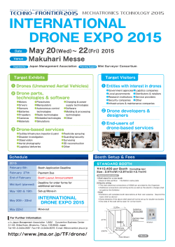


© Copyright 2026