Download Report

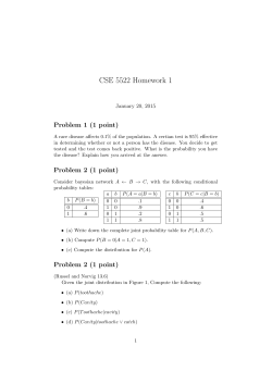
Supporting information for:
Automated Quantitative Image Analysis of
Nanoparticle Assembly
Chaitanya R. Murthy, Bo Gao, Andrea Tao, and Gaurav Arya∗
Department of NanoEngineering
University of California, San Diego
9500 Gilman Drive, Mail Code 0448
La Jolla, CA 92093
E-mail: [email protected]
Phone: 858-822-5542. Fax: 858-534-9553
∗
To whom correspondence should be addressed
S1
Unbiased feature measurement
This section provides a derivation of the exact formula used to calculate bias-correction
weights in our software. We begin with Eq. 1 from the main text, which gives the conditional
probability that an object of fixed orientation will entirely fit within a randomly placed field
of view (and will therefore be measurable), given that its centroid is contained in that field
of view:
(Wx − Fx )(Wy − Fy )
(S1)
P =
Wx Wy
where Wx and Wy are the dimensions of the image in the x and y directions, and Fx and
Fy are the maximum dimensions of the object in those directions. The extent of an object
along some arbitrary direction θ is given by
Fθ = max (~rk · eˆθ ) − min (~rk · eˆθ )
k
k
(S2)
where ~rk is the position vector of point k relative to the centroid of the object and eˆθ is
the unit vector specifying the direction; we define θ as the counterclockwise angle from the
positive x-axis, so that eˆθ = [cos θ, sin θ]. The orientation-averaged conditional probability
that an object i will be measurably contained within a randomly placed field of view is then
given by
h(Wx − Fθ )(Wy − Fθ+ π2 )iθ∈[0,π)
(S3)
hPiθ iθ =
Wx Wy
where the angle brackets denote averaging of the specified variable over the given range, and
only angles smaller than π radians need to be considered in the average because Fθ+π = Fθ .
Taking the inverse of both sides of Eq. S3 yields Eq. 2 in the main text. Eq. S3 can be
rewritten as
hPiθ iθ =
h(Wx − Fθ )(Wy − Fθ+ π2 ) + (Wx − Fθ+ π2 )(Wy − Fθ )iθ∈[0, π2 )
2Wx Wy
=
h2Wx Wy + 2Fθ Fθ+ π2 − (Wx + Wy )(Fθ + Fθ+ π2 )i
2Wx Wy
=
Wx Wy + hFθ Fθ+ π2 i − 12 (Wx + Wy )hFθ + Fθ+ π2 i
Wx Wy
(S4)
where we have grouped terms and expanded the numerator, using the periodicity of Fθ
to again reduce the range of angles considered (all averages here are taken over 0 ≤ θ <
π/2). The code assigns a weight of wi = 1/hPiθ iθ to each measured cluster, where hPiθ iθ is
calculated using Eq. S4.
S2
Empirical distribution of single-particle areas
The formula implemented in our software (Eq. 9 in main text) to estimate cluster size distributions via Bayesian inference makes use of the assumption that the distribution of singleparticle areas is Gaussian. Figure S1 contains a histogram of all particle areas measured
in our aggregation experiment involving Ag nanocubes (E1). The distribution of particle
areas does appear to be very nearly Gaussian; similar results were obtained in the other
experiments that we analyzed.
2200
2000
Histogram of Particle Sizes
Fitted Gaussian
1800
Number of Particles
1600
1400
1200
1000
800
600
400
200
0
2000
4000
6000
8000
Particle Area a/nm
10000
Figure S1: Histogram of particle areas for all particles identified in images taken during our
Ag nanocube aggregation experiment (E1). The red curve is a fitted Gaussian.
S3
Calculation of self-similarity dimensions by regression on cluster data
As discussed in the main text, our software computes various self-similarity dimensions D
by linear regression (LR) on log(s) versus log(l) data, where s is cluster size and l is some
cluster length scale. The corresponding dimension is obtained directly as the slope of such a
fit. An alternative would be to perform non-linear regression (NLR) on the original (not logtransformed) data, and obtain D or its inverse as the exponent in the fitted power law. Xiao
et al. have compared these two methods (LR on log-transformed data versus NLR on the
original data) and have demonstrated that the error distribution may be used to determine
which method to use. S1
We have analyzed the distribution of residuals obtained in both kinds of regression on our
(R)
cluster data. Figure S2 shows regressions aimed at computing the fractal dimension Df ,
which describes the scaling of cluster size s with radius of gyration Rg :
(R)
s ∼ Rg Df
(S5)
The same original dataset is used in each regression, namely data for all clusters observed at
time points t = 173 and 180 minutes in our aggregation experiment involving Ag nanocubes
(E1). In the regressions where Rg or log(Rg ) is on the x-axis, only data for clusters with
Rg > 3r1 are plotted and used in the fits, where r1 is the mean single-particle radius of
gyration for the same experiment. In the regressions where s or log(s) is on the x-axis, only
data for clusters of estimated size s ≥ 4 are plotted and used in the fits. The residuals from
the LRs appear to be homoscedastic (Figure S2b,h) and approximately normally distributed
(Figure S2c,i). By contrast, the residuals from the NLRs are clearly heteroscedastic (Figure S2e,k) and their distribution is not normal (Figure S2f,l). Similar results were obtained
for other experiments, time points, and self-similarity dimensions.
These results strongly suggest that log-transformation and LR is preferable to NLR for
computing self-similarity dimensions from cluster data. We further prefer fitting log(s) versus
log(Rg ) (Figure S2 a-c) rather than the opposite (Figure S2g-i) because in the former the
slope of the fit directly gives the dimension. Similarly, other self-similarity dimensions are
computed as the slopes of linear fits to log(s) versus log(l) data, where l is the appropriate
cluster length scale.
S4
log(s)
5
4
3
2
1
log(s)
b
f(x) = 1.31x − 4.53
Data
0.5
0.25
0
−0.25
−0.5
c
80
# of Residuals
a
60
40
20
Residuals
4.5
5
5.5
6
0
6.5
−0.5 −0.25
log(R/nm)
80
f
200
# of Residuals
d
0
0.25
0.5
5
10
0.2
0.4
log(s)
150
s
60
40
f(x) = 0.0083 x1.36
20
Data
0
10
5
0
−5
−10
s
e
100
50
Residuals
100
200
300
400
500
600
700
0
800
−10
−5
0
R/nm
g
i
7
80
6
f(x) = 0.71x + 3.56
5
# of Residuals
log(R/nm)
log(R/nm)
h
s
Data
4
0.4
0.2
0
−0.2
−0.4
Residuals
1.5
2
2.5
3
3.5
4
60
40
20
0
4.5
log(s)
R/nm
k
l
850
700
550
400
250
100
f(x) = 37.67 x0.69
Data
100
50
0
−50
−100
Residuals
10
20
30
40
50
s
−0.2
0
log(R/nm)
60
70
80
# of Residuals
R/nm
j
−0.4
150
100
50
0
−100 −50
0
50
100
R/nm
Figure S2: Residual analysis of different regressions aimed at calculating the fractal dimen(R)
sion Df from cluster size s and radius of gyration R data. (a) and (g) show linear regressions
(LR) on log-transformed data, while (d) and (j) show nonlinear regressions (NLR). (b), (e),
(h), and (k) show the residuals of each corresponding fit, while (c), (f), (i), and (l) contain
histograms showing the distributions of these residuals. The original data used for each of
the four regressions are identical.
S5
Validation of PICT algorithms
In order to validate our image analysis software, we applied it to various SEM images and
compared the results with those obtained manually or through the use of other software (such
as the popular ImageJ ). Some results from these validation studies are presented below.
Validation of particle detection algorithms
The procedure used by PICT to detect particles is described in Section 2.3 of the main
text. Particles are identified on the basis of three object properties—area, solidity, and
eccentricity—whose acceptable ranges are specified by the user during calibration. Figures S3
and S4 show particles detected by PICT in a particular SEM image taken from the Ag
nanocubes experiment (E1). The property ranges that were used in identifying cubes are
listed in Table 1 in the main text. Note that not all single particles need to be detected, and
that particles forming part of larger clusters may also be detected if they are separated from
nearby particles by small gaps. This behavior is intentional.
Figure S4: Cropped image with detected
particles marked in color. PICT found 514
particles in this image.
Figure S3: An SEM image taken at time
point t = 135 minutes in the experiment involving Ag nanocubes (E1).
Validation of algorithms for identifying clusters
The procedure used by PICT to identify clusters is described in Section 2.3 of the main text,
and involves a morphological closing operation with a small structuring element. This joins
any particles that are not quite touching, yet are close enough to be considered part of a
cluster. The user may specify the gap below which particles are joined in this manner (by
specifying the radius rS of the structuring element in nanometers). Different specifications
can lead to a group of particles being identified either as a single cluster, or as multiple
clusters. We have found that a good choice for rS is half the distance between an average
pair of NPs in a cluster (as determined beforehand by manual inspection and measurement).
Figures S5 and S6 show clusters identified by PICT in a particular SEM image taken
from the Ag nanocubes experiment (E1), using a value of rS = 42nm. Any border-touching
S6
clusters are ignored, as discussed in Section 2.4 of the main text. Figures S7 and S8 show
clusters identified in an image taken from the experiment involving 13nm Au nanospheres
(E3). Note that the nanospheres are often separated by significant gaps even when they
are part of a single cluster. To account for this, we used a value of rS = 12nm, which is
approximately twice the radius of a bare sphere.
Figure S5: An SEM image taken at time
point t = 180 minutes in the experiment involving Ag nanocubes (E1).
Figure S6: Cropped image with identified
clusters marked in color. Each continuous
colored region is one cluster.
Figure S7: An SEM image taken at time
point t = 85 minutes in the experiment involving 13nm Au nanospheres (E3).
Figure S8: Cropped image with identified
clusters marked in color. Each continuous
colored region is one cluster.
Validation of cluster property calculations
The methods used to calculate cluster properties are discussed in Sections 2.5-2.8 of the
main text. In order to validate these methods, we compared the PICT results against
S7
those obtained from visual inspection of the images and from analysis using the popular
ImageJ software. Validation results for a particular SEM image taken from the Ag nanocubes
experiment (E1) are shown below. Figure S9 is the original SEM image, while Figure S10
is a cropped and binary-transformed version that was imported into ImageJ and analyzed.
Note that a few extra white pixels had to be added to this binary image so that ImageJ
would correctly identify each cluster as a single object. All identified clusters are marked
and those above a size threshold, numbered, in Figure S11. Figure S12 shows the calculated
backbones and fitted ellipses for these clusters; these may be verified by visual inspection.
Some other computed cluster properties are listed in Table S1 and compared with values
obtained via hand-counting or from ImageJ.
Figure S9: SEM image taken at time point
t = 188 minutes in the experiment involving
Ag nanocubes (E1).
Figure S10: Cropped, binary-transformed
image with border-touching clusters removed. This was analyzed with ImageJ.
Figure S11: Valid clusters identified by
PICT (48 in all) are marked in blue. Clusters of estimated size s ≥ 4 are numbered.
Border-touching clusters are marked in red.
Figure S12: Cluster backbones (red) and fitted ellipses (blue), as determined by PICT,
are shown for all clusters that are numbered
in Figure S11.
S8
Table S1: Comparison of PICT results with hand-counting (count) and ImageJ (ImJ) results
for some basic cluster properties. The clusters are those that are numbered in Figure S11. s
is the true cluster size, while s˜ is an estimate computed using Eq. 6 in the main text. Note
that s˜ is not directly used by PICT in calculating size statistics. AR is the aspect ratio.
Cluster #
1
2
3
4
5
6
7
8
9
10
11
13
14
15
16
17
18
19
20
21
23
25
26
27
28
29
30
31
32
34
35
36
37
38
39
40
41
42
43
44
45
46
s˜ (PICT)
5.4
5.0
15.7
13.1
29.0
13.0
45.3
6.8
21.3
13.7
17.4
36.7
10.1
8.6
14.1
4.7
37.3
8.4
6.9
10.0
9.3
15.1
4.7
41.4
39.2
4.2
9.5
20.4
28.9
15.8
4.3
6.7
26.8
6.7
11.9
40.7
7.8
7.6
12.9
4.5
16.1
11.0
s (count)
6
5
16
14
29
14
46
6
22
14
17
38
11
8
15
5
37
9
7
10
9
16
5
43
38
4
10
22
28
16
4
7
26
7
12
38
7
8
13
4
16
10
AR (PICT)
1.506
3.149
1.661
3.215
1.721
1.671
2.755
1.486
2.098
3.615
2.125
1.932
1.963
1.567
4.929
2.384
2.204
2.232
2.218
2.092
2.543
4.657
3.961
3.194
2.210
3.431
1.318
2.419
4.089
3.169
2.555
2.094
2.384
2.052
1.847
3.640
1.431
1.647
2.566
1.955
2.200
2.146
S9
AR (ImJ)
1.502
3.160
1.666
3.211
1.720
1.677
2.761
1.486
2.095
3.617
2.125
1.931
1.951
1.581
4.996
2.399
2.201
2.233
2.224
2.080
2.568
4.702
3.974
3.166
2.231
3.445
1.313
2.440
4.111
2.551
3.190
2.124
2.399
2.065
1.848
3.673
1.431
1.647
2.584
1.957
2.202
2.121
Solidity (PICT)
0.53
0.55
0.37
0.35
0.25
0.36
0.19
0.56
0.31
0.48
0.29
0.23
0.40
0.43
0.40
0.53
0.29
0.50
0.45
0.52
0.48
0.35
0.57
0.30
0.26
0.59
0.52
0.37
0.26
0.30
0.64
0.52
0.28
0.59
0.47
0.20
0.53
0.40
0.37
0.70
0.28
0.52
Solidity (ImJ)
0.51
0.53
0.38
0.35
0.26
0.36
0.20
0.53
0.31
0.48
0.30
0.23
0.40
0.44
0.41
0.51
0.30
0.51
0.43
0.51
0.48
0.36
0.56
0.31
0.26
0.56
0.52
0.38
0.27
0.62
0.30
0.53
0.28
0.60
0.47
0.20
0.53
0.40
0.36
0.68
0.28
0.53
Validation of Bayesian algorithm for computing cluster size statistics
The Bayesian algorithm used by PICT to calculate cluster size distributions is described in
Section 2.5 of the main text. In order to validate this algorithm, we selected a subset of the
SEM images from our Ag nanocubes experiment (E1); three images were chosen at each of
the time points t = 127, 135, 143, 150, 158 and 165 minutes. For these images, we manually
identified all clusters and found their sizes (by counting the number of particles making
up each cluster). This data was then used to compute the relative size distribution νs (t)
(see Eq. 3 in the main text). Figure S13 compares the manual result with the distributions
calculated by PICT from the same set of images.
a
b
t = 127 minutes
0
0
10
−1
−1
−3
−1
s
−2
10
−3
10
−4
10
−4
1
2
3
4
−4
10
5
1
2
s
e
10
4
10
5
PICT
Manual
−1
f
t = 158 minutes
0
PICT
Manual
−1
−3
−2
s
10
15
10
PICT
Manual
−2
10
10
−4
10
5
−3
10
−4
4
t = 165 minutes
0
−1
−3
10
3
10
ν (t)
νs(t)
−2
10
5
2
10
10
0
1
s
10
10
νs(t)
3
s
t = 150 minutes
0
−2
10
−3
10
10
PICT
Manual
10
ν (t)
νs(t)
νs(t)
−2
10
10
PICT
Manual
10
10
t = 143 minutes
0
10
PICT
Manual
10
d
c
t = 135 minutes
−4
0
5
10
s
s
15
20
10
0
5
10
15
s
Figure S13: Comparison of relative size distributions νs (t) calculated by PICT (green line)
and manually (black dots) for a particular set of SEM images. Three images were analyzed at
each time point; these images are from our Ag nanocubes experiment (E1). The lighter green
regions are error bounds returned by PICT; these are not plotted for sizes where the predicted
value is smaller than the error. Agreement between the results is in general excellent; slight
deviations are due to the bias-correction algorithms used by PICT (see Section 2.4 in the
main text), or simply due to statistical fluctuations (from lack of data) at large cluster sizes.
S10
20
References
(S1) Xiao, X.; White, E. P.; Hooten, M. B.; Durham, S. L. On the use of log-transformation
vs. nonlinear regression for analyzing biological power laws. Ecology 2011, 92, 1887–94.
S11