1. No category

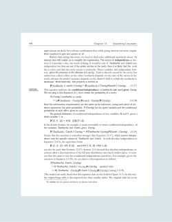
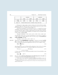
CSE 5522 Homework 1
January 20, 2015
Problem 1 (1 point)
A rare disease affects 0.1% of the population. A certian test is 95% effective
in determining whether or not a person has the disease. You decide to get
tested and the test comes back positive. What is the probability you have
the disease? Explain how you arrived at the answer.
Problem 2 (1 point)
Consider bayesian network A ← B → C, with the following conditional
probability tables:
a b P (A = a|B = b)
c b P (C = c|B = b)
b P (B = b)
0 0
.1
0 0
.4
0
.4
1 0
.9
1 0
.6
1
.6
0 1
.2
0 1
.5
1 1
.8
1 1
.5
• (a) Write down the complete joint probability table for P (A, B, C).
• (b) Compute P (B = 0|A = 1, C = 1).
• (c) Compute the distribution for P (A).
Problem 2 (1 point)
(Russel and Norvig 13.6)
Given the joint distribution in Figure 1, Compute the following:
• (a) P (toothache)
• (b) P (Cavity)
• (c) P (T oothache|cavity)
• (d) P (Cavity|toothache ∨ catch)
1
L
L
toothache
catch catch
L
catch
L
toothache
catch
cavity
.108 .012
.072 .008
cavity
.016 .064
.144 .576
2
Problem 2 (2 points)
Derive the maximum likelihood estimate (MLE) for the mean of a Gaussian
distirbution with fixed variance. Solve the equation:
∂ log P (D|µ, σ)
∂µ
= 0
Problem 3 - Programming Project (5 points)
(Taken from CSE 515 at the University of Washington)
Implement the EM algorithm for mixtures of Gaussians. You can use
C, C++, Java, C#, Matlab, or Python. Assume that means, covariances,
and cluster priors are all unknown. For simplicity, you can assume that
covariance matrices are diagonal (i.e., all you need to estimate is the variance
of each variable). Initialize the cluster priors to a uniform distribution and
the standard deviations to a fixed fraction of the range of each variable.
Your algorithm should run until the relative change in the log likelihood of
the training data falls below some threshold (e.g., stop when log likelihood
improves by < 0.1%). The program should be run on the command line
with the following arguments:
./gaussmix <\# of cluster> <data file> <model file>
It should read in data files in the following format:
<\# of examples> <\# of features>
<ex.1, feature 1> <ex.1, feature 2> . . . < ex.1, feature n>
<ex.2, feature 1> <ex.2, feature 2> . . . < ex.2, feature n>
. . .
And output a model file in the following format:
<\# of clusters> <\# of features>
<clust1.prior> <clust1.mean1> <clust1.mean2> . . . <clust1.var1> . . .
<clust2.prior> <clust2.mean1> <clust2.mean2> . . . <clust2.var1> . . .
. . .
Train and evaluate your model on the Wine dataset, available from the
course Web page. Each data point represents a wine, with features representing chemical characteristics including alcohol content, color intensity,
hue, etc. We provide a single default train/test split with the class removed
to test generalization. You can find the full dataset and more information
in the UCI repository (linked from the course Web page). Start by using 3
3
clusters, since the Wine dataset has three different classes. Evaluate your
model on the test data.
Two recommendations:
• To avoid underflows, work with logs of probabilities, not probabilities.
• To compute the log of a sum of exponentials, use the log-sum-exp trick:
P
P
log i exp(xi ) = xmax + log i exp(x − xmax )
Answer the following questions with both numerical results and discussion.
• (a) Plot train and test set likelihood vs. iteration. How many iterations does EM take to converge?
• (b) Experiment with two different methods for initializing the mean
of each Gaussian in each cluster: random values (e.g., uniformly distributed from some reasonable range) and random examples (i.e., for
each cluster, pick a random training example and use its feature values as the means for that cluster). Does one method work better than
the other or do the two work approximately the same? Why do you
think this is? (Use whichever version works best for the remaining
questions.)
• (c) Run the algorithm 10 times with different random seeds. How
much does the log likelihood change from run to run?
• (d) Infer the most likely cluster for each point in the training data.
How does the true clustering (see wine-true.data) compare to yours?
• (e) Graph the training and test set log likelihoods, varying the number
of clusters from 1 to 10. Discuss how the training set log likelihood
varies and why? Discuss how the test set log likelihood varies, how it
compares to the training set log likelihood, and why. Finally, comment
on how train and test set performance with the true number of clusters
(3) comapres to more and fewer clusters and why.
4