
Baseline Energy Modeling Approach for Residential M&V Applications
May 11, 2015 REPORT #E15-288 Baseline Energy Modeling Approach for Residential M&V Applications Prepared by: Eliot Crowe, Alex Reed, Hannah Kramer, Joan Effinger, Emily Kemper, and Mary Hinkle CLEAResult 100 SW Main St., Suite 1500 Portland, OR 97204 Northwest Energy Efficiency Alliance PHONE 503-688-5400 FAX 503-688-5447 EMAIL [email protected] Baseline Energy Modeling Approach for Residential M&V Applications Table of Contents Executive Summary ......................................................................................................................... i 1. Introduction ................................................................................................................................1 1.1. Background........................................................................................................................1 1.2. Project Overview ...............................................................................................................3 2. Methodology ..............................................................................................................................5 2.1. Literature Review ..............................................................................................................5 2.2. Individual Home Regression Analysis ..............................................................................5 2.2.1. Development of Analysis Dataset .........................................................................5 2.2.2. Development of Regression Model Specification .................................................6 2.2.3. Metrics Used to Determine Regression Model Quality ........................................7 2.2.3.1. Mean Bias Error (MBE) ...................................................................................... 7 2.2.3.2. Detectable Percent Savings ................................................................................. 8 2.2.4. Exploration of Model Input Variations .................................................................9 2.3. Pooled Data Analysis ......................................................................................................10 2.4. HEMS Industry Research ................................................................................................10 3. Findings....................................................................................................................................12 3.1. Literature Review ............................................................................................................12 3.1.1. EM&V Sampling Approach ................................................................................12 3.1.2. Data Interval ........................................................................................................13 3.1.3. NEEA Residential Building Stock Assessment (RBSA) Metering Study ..........13 3.1.4. Barriers and Challenges .......................................................................................14 3.1.5. Summary of Literature Review Findings ............................................................14 3.2. Individual Home Baseline Regression Development ......................................................15 3.2.1. Model Specification and Initial Results ..............................................................15 3.2.2. Comparison of Hourly and Daily Regression Models ........................................18 3.2.3. Impact of Varying Confidence Levels ................................................................19 3.2.4. Impact of Part-Year Modeling and Seasonality ..................................................20 3.3. Pooled Interval Data Baseline Regression Analysis .......................................................24 3.4. HEMS Industry Research ................................................................................................26 4. Conclusions and Recommendations ........................................................................................28 4.1. Conclusions .....................................................................................................................28 4.2. Recommendations ...........................................................................................................29 5. References ................................................................................................................................31 Appendix A: Literature Review Summary Table ............................................................................0 Appendix B: Detectable Percent Savings for Part-Year Models ...................................................15 Baseline Energy Modeling Approach for Residential M&V Applications Table of Figures Figure 1. Example Data from a Home in the RBSA Dataset, Showing Hourly Energy Consumption Values and the Baseline Regression Developed Under This Project ..................... 16 Figure 2. Detectable Percent Savings for Each Home in the Study Dataset (90% Confidence Level) ............................................................................................................................................ 17 Figure 4. Detectable Percent Savings for Hourly and Daily Models at 90 % Confidence Level . 19 Figure 5. Detectable Percent Savings at Varying Confidence Levels .......................................... 20 Figure 6. Mean Bias Errors for Three-Month Models .................................................................. 21 Figure 7. Mean Bias Errors for Six-Month Models ...................................................................... 23 Figure 8. Mean Bias Errors for Nine-Month Models ................................................................... 24 Figure 9. Pooled Baseline Modeling Results ................................................................................ 25 Figure 10. Detectable Percent Savings for Three-Month Models ................................................ 15 Figure 11. Detectable Percent Savings for Six-Month Models .................................................... 15 Figure 12. Detectable Percent Savings for Nine-Month Models .................................................. 16 Baseline Energy Modeling Approach for Residential M&V Applications Executive Summary The growing availability of electric interval data from smart meters is driving development of consumer-facing analytical software that utilizes those data. Analytical software that could utilize interval data to offer automated measurement and verification (M&V) of savings from energy efficiency projects would present several opportunities to utilities, including: Supporting financial transactions based on measured energy savings Allowing for a greater variety of program measures Determining interim savings estimates for program implementation Providing ongoing monitoring/feedback for utility customers Under this project, CLEAResult addressed some of the technical research questions that will support progress toward an automated M&V approach for individual homes using interval data. Establishing a method for developing a robust energy baseline is a fundamental first step, as this can be combined with post-implementation energy use to determine energy savings. The primary goal of the project was to establish a method for developing a robust energy baseline regression model and to evaluate how that model performed on a sample dataset. To achieve that goal, the Northwest Energy Efficiency Alliance (NEEA) contracted with CLEAResult to conduct a literature review, baseline regression modeling analysis, and a high-level review of home energy management system (HEMS) M&V capabilities. Literature Review The project team gained useful insights from the literature review on what will be needed for development of an automated M&V approach. Overall, the literature review indicated that statistical modeling using meter data at a daily interval is possible, but that using intervals smaller than a day is a new approach unproven for residential applications. Additionally, current residential program evaluation approaches quantify average savings for a group of homes, rather than for individual homes. Individual Home Baseline Regression Modeling In order to develop a specification for a robust baseline modeling approach, the project team first established two key metrics that could be used to evaluate the quality of different model types: mean bias error (MBE) and detectable percent savings, described in Section 2.2.3 of this report. For model specification, the team chose to perform piecewise regression modeling using outdoor air temperature, day of week, and time of day as independent variables, with correction for autocorrelation. After finalizing the regression model specification, they assessed the impact of varying analysis time intervals, confidence levels, and monitoring periods on model quality. The team obtained the data used for this project via NEEA’s Residential Building Stock Analysis (RBSA) metering study. The team used the data from the ninety-six viable RBSA study homes to develop two separate datasets for this study, based on 1) hourly consumption values and 2) daily consumption values, and developed hourly and daily baseline regression models for each home in the study dataset. NEEA - i Baseline Energy Modeling Approach for Residential M&V Applications The hourly models yielded a median value for detectable percent savings of 3.6%, compared to 4.3% for the daily models; the latter also had a wider distribution. Given that a low detectable percent savings value is desirable, program applications would benefit from a lower detectable percent savings; thus the project team used hourly models for all subsequent analyses under this project. As the project team expected, the detectable percent savings increases as the confidence level increases. The three confidence levels (80%, 90%, 95%) evaluated in this study yielded relatively small differences in median value, ranging from 2.8% at the 80% confidence level to 4.3% at the 95% confidence level. The increase in distribution is significant, however. In addition to the median value, the project team determined the 75th and 90th percentile values for the homes in the dataset. At the 90th percentile, the detectable percent savings at 80% confidence level is 5.0%, compared to 7.6% at 95% confidence level. The team also developed a series of part-year models for individual homes using three, six, and nine months of data, all of which showed detectable percent savings similar to those of the fullyear savings approaches (see Appendix B). The team focused on mean bias error (MBE) for the part-year analyses to determine the degree to which shortening the monitoring period introduces bias into the results (an MBE value of zero is ideal). The three-month models yielded unacceptably high MBE values and had a broad distribution. The six-month models showed improvement in MBE and might be suitable for automated M&V depending on the expected level of savings. The MBE values for the nine-month models are sufficiently low that these models could probably be used to claim annualized savings in most cases (see Figure 8 in Section 3.2.4). Pooled Interval Data Baseline Regression Analysis Following the individual home analysis, the project team developed a series of “pooled models,” in which it aggregated all data from a group of homes into a single dataset and developed a single regression model. The project team developed pools of ten, twenty, fifty, and all ninety-six homes, which produced relatively consistent detectable percent savings values from 3.7% to 4.6% (at a confidence level of 90%). These pooled detectable percent savings values were similar to the median value of the individual homes within each given pool, and are an improvement on the 75th percentile and 90th percentile values. Conclusions and Recommendations The results of the analytical research under this project provide a strong foundation for future efforts toward an automated M&V approach using interval data. The baseline regression analysis for individual homes yielded encouraging results with respect to the key quality metrics and the relative ease of model generation once the project team had developed the model specification. The individual home analysis results provide guidance on the expected accuracy of baseline regressions based on the required confidence level, post-implementation data duration, and the proportion of homes targeted within a population. The project team’s analysis also aided understanding of the relative levels of uncertainty in individual models and pooled models of different sizes. NEEA - ii Baseline Energy Modeling Approach for Residential M&V Applications The literature review under this project confirmed the team’s initial belief that M&V approaches for residential applications using interval data have not yet been applied. The HEMS research uncovered no instances of products performing utility program M&V, although it identified two tools with some level of savings estimation capability. The findings from this project constitute a promising first step along the road to automated M&V using interval data. Recommendations for future efforts include technical research toward a robust M&V methodology, market research to establish a range of program applications that can meet regulatory requirements, and development of industry guidance to support scalable analytics solutions. NEEA - iii Baseline Energy Modeling Approach for Residential M&V Applications 1. Introduction The growing availability of electric interval data from smart meters is driving development of consumer-facing analytical software that utilizes those data. This raises the possibility that analytical software could offer automated measurement and verification (M&V) of savings from energy efficiency projects. Such a capability would present several opportunities, including: Supporting a shift in utility program approach from estimated savings to measured savings, whereby program incentives are allocated based on a pay-for-performance basis Allowing for a greater variety of measures, including behavior and controls approaches for which it can be difficult to determine savings Determining interim savings estimates for program implementation to provide insights into which homes are saving more than others and which strategies are most successful in driving energy use reductions. Implementers can use these insights to support mid-course improvements to program design and marketing approaches Providing ongoing monitoring/feedback for consumers. Once an energy use baseline is created, it can be compared to current energy use for ongoing tracking of savings. Communicating energy savings more dynamically to customers supports both behavior savings and re-engagement in programs to achieve deeper savings This project set out to answer some of the technical research questions that must be addressed to support progress toward an automated M&V approach for individual homes using interval data. 1.1. Background Quantifying the impacts of an energy efficiency project is important to parties with a financial stake in the project investment. This can include utility ratepayers (homeowners and/or tenants), utilities providing incentives toward the project, and third parties providing financing for the project. Quantifying the energy that did not get used as a result of a project is notoriously challenging, however, due to the dynamic nature of the manner in which buildings consume energy. Established methods for quantifying energy impacts fall into four main categories, each with its own limitations, as Table 1 summarizes. NEEA - 1 Baseline Energy Modeling Approach for Residential M&V Applications Table 1. Established Methods for Quantifying Project Energy Impacts Method Deemed savings Engineering calculations Statistical modeling Simulation Limitations Not based on “as-found” conditions; highly dependent on engineering assumptions; may be relatively accurate for a population, but not intended to be accurate for an individual building. Difficult to balance accuracy with complexity/cost; no actual measurement of energy consumption or quantification of uncertainty in savings; dependent on engineering assumptions for which it is difficult to capture interactive and behavioral effects; may need system monitoring to confirm assumptions. Industry-accepted methods are based on having at least twelve months of pre- and post-implementation monthly energy consumption data and are not considered suitable for projects with less than ten percent whole building savings; requires utility regulatory acceptance of claiming savings at the meter level rather than measure level. Site-specific simulations require high labor input and high skill level; can be challenging or impossible to capture operational and behavior-based improvements; may or may not be calibrated to actual energy usage. The growth in availability of smart meter data and commercially-available analytical tools shows potential for addressing the limitations noted above for statistical modeling. An automated M&V method would allow for implementation of a variety of measures such as behavior and controls for which it has to date been difficult to accurately determine savings. The Northwest Energy Efficiency Alliance (NEEA) recognizes the opportunity to develop an automated M&V approach that supports financial transactions and utility program savings claims. Reaching that goal will require a multi-faceted effort to address technical and market barriers, including development of a standard methodology and subsequent validation of analytical tools that can automate that methodology. The term “automated M&V” does not have an industry-accepted definition. For the purposes of this project it is defined as an M&V method that can quantify electric savings, relative to a predefined baseline period, with the user entering only the post-implementation period start and end dates. The project team assumes that the M&V tool will have automated access to electric interval data and to outside air temperature data. It also assumes that the tool would be initially configured to ensure that the baseline model meets specified requirements for accuracy (these requirements would vary depending on the program approach and rigor). Past and ongoing research on commercial applications suggests that M&V utilizing interval data can be used to quantify savings of less than ten percent and with less than a year of postimplementation data (Effinger, Effinger, Friedman 2012; Katipamula et al. 1993). Preliminary research also documents the potential for analytical software tools (known as energy management and information systems, or EMIS) to automate M&V (Crowe, Kramer, Effinger 2014; Kramer et al. 2013). However, virtually no documented research exists on residential M&V methods using interval data or the analytical capabilities of residential analytical software tools (which fall into the class of home energy management systems, or HEMS). NEEA - 2 Baseline Energy Modeling Approach for Residential M&V Applications Achieving an automated M&V approach for residential applications requires a fundamental first step of establishing a method for developing a robust energy baseline, which could potentially be combined with post-implementation energy use to quantify the impacts of energy-saving actions for an individual home. A parallel need exists to review the analytical capabilities of commercially-available HEMS to understand whether these tools have automated M&V functionality. HEMS research to date has typically focused on these tools’ ability to drive energy-saving actions rather than to quantify the impacts of those actions. As NEEA seeks to transform the market, understanding if and how HEMS vendors may implement automated M&V approaches is important, as widespread market adoption would require a scalable technology solution. 1.2. Project Overview NEEA initiated this project in order to develop a technical foundation for development of an automated M&V approach for residential applications using interval data. The goals of the project were to: Understand how (if at all) interval data has been used for quantifying project energy savings in the residential sector Establish a method for developing a robust energy baseline regression model and determine how well those models perform Gain a high-level understanding of M&V capabilities within commercially-available HEMS software In order to achieve the project goals, NEEA contracted with CLEAResult to complete the following research activities: A literature review that documents existing research and industry best practices on datadriven M&V for residential applications Development of individual home baseline regression models for approximately one hundred homes and reporting of statistical metrics for the models Development of baseline regression models using aggregated interval data from groups of homes (referred to as “pooled models”) A high-level review of HEMS tools to identify M&V approaches that utilize interval data As noted earlier, the long-term vision of developing an automated M&V approach will require the resolution of a complex set of barriers and research questions. Analytical research questions applicable to this project included: What model specification and data inputs best suit residential interval data analysis? What level of uncertainty exists in baseline regression models for individual homes? What is the minimum percent savings that could be detected for an individual home using interval data-driven M&V? How does post-implementation monitoring period length and seasonality affect model uncertainty? What impact does pooling interval data have on model uncertainty? NEEA - 3 Baseline Energy Modeling Approach for Residential M&V Applications Are there any screening criteria that can improve model results or help to eliminate data for homes that are unsuited to an automated M&V approach? Answering these questions can produce insights regarding the applicability of automated M&V using interval data for residential applications. For example, regression model uncertainty affects the minimum percent savings that could be detected using interval data modeling – lower uncertainty in the baseline model means that a lower percent savings could be detected. This is important because the percent savings that can be detected impacts the types of projects and programs to which the methodology might apply. NEEA - 4 Baseline Energy Modeling Approach for Residential M&V Applications 2. Methodology The research methodologies employed in each of the main research tasks are described below. 2.1. Literature Review The literature review for this project targeted publications that documented the state of the art in residential M&V using hourly or monthly energy data, covering industry best practice as well as a variety of typical approaches. The scope of the literature search included documents relating to project-specific M&V approaches as well as independent formal evaluations conducted on whole programs (EM&V). While this project strongly focused on the use of interval data for residential M&V, the project team did not anticipate that the literature search would uncover many documents on that narrow topic; as a result, the search targeted residential M&V applications that used energy consumption data of any frequency. The team further expanded the search to capture some documents associated with residential interval data analytics unrelated to M&V, such as market segmentation analysis. The project team’s literature search uncovered seventeen relevant documents, including formal program evaluations, research papers, and industry guidelines. It also included a report on the metering study for a subset of the homes included in NEEA’s Residential Building Stock Assessment (Larson et al. 2014) (the same dataset used for the data analysis under this project). The project team created two summaries based on the literature review: 1) a summary of key findings, barriers, and challenges related to residential data-driven M&V and 2) a literature review summary table (Appendix A) covering findings from each individual document. 2.2. Individual Home Regression Analysis The project team conducted the data analysis under this project with the primary goal of evaluating the applicability of using electric interval data to develop a baseline regression model that could form a foundation for an automated M&V approach. The team divided the data analysis effort into two tasks: 1) evaluating the potential of developing a baseline regression for an individual home, and 2) evaluating a pooled approach, which is described in the next section. Given the lack of prior documented research on the topic of individual home regression analysis using interval data, the research under this project was exploratory in nature. The project team conducted the analysis to understand how different factors affect the quality of individual home regressions, as opposed to establishing a definitive protocol that would require more industry stakeholder input. 2.2.1. Development of Analysis Dataset The dataset utilized for this project was the same as that used for the RBSA metering study. NEEA provided the following data to the project team: Fifteen-minute electric interval data (kWh) for 103 single-family homes distributed across Oregon, Washington, Idaho, and Montana Outside air temperature data (°F, dry bulb) NEEA - 5 Baseline Energy Modeling Approach for Residential M&V Applications A spreadsheet of physical characteristics and other general information for each of the homes in the dataset The project team selected the RBSA dataset for this project primarily for cost reasons; defining a new sample set, collecting new data, and assuring the quality of those data would have added significant cost to the project. The RBSA data also provided a secondary benefit, in that NEEA published detailed analyses at the end-use level for the dataset and home characteristics as part of the metering study; the team thought that this could provide helpful insights when reviewing baseline regression models developed under this project. Upon inspection, the project team found that seven of the homes had either no energy data or no weather data, and these were excluded from further analysis. The team used data from the remaining ninety-six homes to develop two separate datasets for this study: one with data rolled up to hourly consumption values, and a second with data rolled up to daily values. The homes in the RBSA dataset spanned a range of sizes and total annual consumption values. In order to support comparison and charting of research results across the dataset, the project team converted each home’s energy consumption data to kWh-per-square-foot values. 2.2.2. Development of Regression Model Specification As noted earlier, little or no published technical research exists on regression modeling of residential interval data. However, the project team has prior experience with efforts in the commercial sector, and is familiar with examples of relevant research published by other organizations (Price et al. 2013). Where possible, the project team aligned with these related efforts in the commercial sector in developing model specifications for this project. Multivariate regression is the most widely-accepted method for creating energy models for individual buildings using actual consumption data for M&V purposes. It is described in the American Society of Heating, Refrigerating and Air-Conditioning Engineers (ASHRAE) Guideline 14 and in the International Performance Measurement and Verification Protocol (IPMVP). The goal of developing the model specification was to choose the type of multivariate regression and the independent variables that generate the lowest uncertainty in the model. The team conducted all modeling using a statistical analysis software package in which it manually developed code. Once the team had developed the software code, it could create models for all ninety-six homes in a single batch. An iterative process of modeling and revising the model specification continued through several rounds, exploring different specification design elements and factors, as shown in Table 2 below. The project team reviewed the model’s uncertainty for each iteration (see Section 2.2.3 for an explanation of key quality metrics). NEEA - 6 Baseline Energy Modeling Approach for Residential M&V Applications Table 2. Model Specification Options Considered Specification Design Element Description Model type Specification of the type of multivariate regression Independent variables Primary data inputs to the regression model; the most likely determinants of energy consumption Factors Considered Five-parameter linear change-point regression Piecewise linear regression Outdoor air temperature (°F) Day of week Time of day Holiday Interaction between day of week and time of day Piecewise regression modeling using outdoor air temperature, day of week, and time of day as independent variables resulted in the highest-quality model. This specification is similar to one of the best-performing models in PG&E’s commercial baselining study (Carrillo et al. 2013), the “time-of-week and temperature regression.”1 The project team members also tested for autocorrelation2 and found significant autocorrelation to be present; they therefore applied the correction approach outlined in ASHRAE Guideline 14 (ASHRAE 2002). 2.2.3. Metrics Used to Determine Regression Model Quality A variety of statistically-derived metrics may be used to evaluate the quality of a regression model. The two selected metrics used for this project are described below. 2.2.3.1. Mean Bias Error (MBE) Mean bias error (MBE) denotes the percentage by which a regression model’s predicted energy use differs from the actual consumption over a defined period. A positive MBE means the modeled energy use for the period is higher than actual use, and a negative MBE means it is lower. An MBE value of zero is ideal. The level of MBE that is “acceptable” is ultimately defined by the user. ASHRAE Guideline 14 states that “models are declared to be calibrated if they produce MBEs within 10% when using hourly data” (ASHRAE 2002). However, if a project is expected to achieve less than ten percent savings (a behavior-based energy efficiency project, for example), an MBE of ±10% would be impractical. For this project the team calculated the MBE for a full year of actual consumption data compared to model predictions for that same period. 1 The final model specification includes only hour-of-day and day-of-week rather than the more granular time-ofweek. The project team tested time-of-week and found that, for its dataset, the reduced degrees of freedom from the additional independent variables outweighed any additional predictive ability. 2 A measure of the extent to which an observation is dependent on its immediate successor, such as the temperature one day being correlated with the temperature the previous day NEEA - 7 Baseline Energy Modeling Approach for Residential M&V Applications 2.2.3.2. Detectable Percent Savings As noted in the Introduction, M&V approaches based on monthly energy regression modeling may generally be used when energy savings are at least ten percent of whole-building energy use. An M&V method based on interval data modeling has the potential to detect a lower percent savings, as evidenced by several research studies (Dethman, Stewart, Duncan 2013; Effinger, Effinger, Friedman 2012; Katipamula, Reddy, Claridge 1994). Evaluating that potential was one of the key goals of this project. When data are available for the entire reporting period, the project team employed an “avoided energy use” approach. For example, if a program is reporting first-year savings and a full year of post-implementation data are available, then the team used the avoided energy use approach. The avoided energy use method involves the creation of a baseline regression using actual consumption data prior to implementation. The actual values of the independent variables recorded during the post-implementation period are then used in the regression to create an adjusted baseline. The adjusted baseline is a prediction of how the home would have operated had the energy efficient change not been implemented. The difference between the adjusted baseline and measured post-implementation energy use is the avoided energy use (Equation 1). Equation 1 When data are not available for the entire reporting period, the team employed a “normalized energy use” approach – for example, if three months of post-implementation data are available for reporting annual savings or if one year of data are available for reporting more than one year of savings (such as savings for the useful life of the implemented measure). The team calculated normalized savings using separate regressions for the baseline and post-implementation periods. Each regression is then driven with a common dataset, such as Typical Meteorological Year (TMY) temperature data. In order to have high confidence that a project has achieved the estimated energy savings, actual energy use in the post-implementation period should be statistically different from the adjusted baseline. In this application, this means that the actual energy use in the post-implementation period should be outside the uncertainty bands of the adjusted baseline. Equation 2 describes this relationship. Equation 2. Post installation energy use ≤ adjusted baseline - RMSE * z-score Where: RMSE = Root mean square error of the regression (a measure of the difference between the model predictions and the actual values) Z-score= The critical value of a normal distribution and confidence level. The z-score is 1.282 for 80% confidence level, 1.645 for 90% confidence level, and 1.960 for 95% confidence level The choice of confidence level is driven by the level of certainty required for the reported savings. NEEA - 8 Baseline Energy Modeling Approach for Residential M&V Applications The ability of an M&V method to measure savings with a high degree of confidence is primarily driven by a relationship between model uncertainty and the magnitude of savings being measured. The project team derived a metric for the minimum percent savings that could be detected from each baseline model’s uncertainty statistics, as described below. Given that the RBSA dataset did not include any post-implementation data, the project team could not directly use Equation 2. It did, however, determine RMSE for each home’s baseline regression model. From this it determined the uncertainty band for each model and estimated the minimum reduction of post-implementation energy use that would be needed to achieve statistical significance; this metric is referred to as the “detectable percent savings.” Equation 3. Detectable percent savings = RMSE * z-score 2.2.4. Exploration of Model Input Variations Once the project team finalized the regression model specification and determined the key quality metrics, the project team assessed the impact of varying analysis time intervals, confidence levels, and monitoring periods on model quality: Analysis Time Interval. As noted earlier, the team derived hourly and daily interval data for each home from the raw RBSA dataset and used it to develop two separate baseline models for each of the ninety-six homes. Confidence Level. A confidence level refers to the percentage of all possible samples for which the calculated confidence interval – a range such as 500 kWh ± 400 kWh – includes the true value – for example, the exact achieved energy savings. A 95% confidence level implies that 95% of the confidence intervals would include the true value. A higher confidence level provides a higher level of assurance that the confidence interval is wide enough to include the true value. The team used confidence levels of 80%, 90%, and 95% for the regression models developed under this project with the intention of providing an indication of the detectable percent savings across a range of applications that can have varying levels of rigor. Monitoring Period Length and Seasonality. The team developed model variants using less than a year of baseline data. The project team divided data into all possible contiguous three-month, six-month, and nine-month season groups, following meteorological seasons: o Winter: December to February o Spring: March to May o Summer: June to August o Fall: September to November For each of the season groups, the project team created a regression using the final model specification described in Table 2. The team then used a modified normalized savings approach to determine the percent savings needed for statistical significance. In this modified normalized savings approach, the team derived the regression model created using less than one year of data NEEA - 9 Baseline Energy Modeling Approach for Residential M&V Applications with the full year of TMY3 data and then used Equation 3 to determine the detectable percent savings. 2.3. Pooled Data Analysis At the project outset, the team did not know whether an individual home approach to M&V using interval data would be feasible, what level of savings would be detectable, and whether that level of savings would be low enough to allow for the various program types discussed in the Introduction. In addition, an individual home approach may not be the ideal M&V approach for programs targeting a community or group of projects. As a result, the project scope included a pooled regression modeling exercise alongside the individual home analysis. A pooled model aggregates all of the data from a group of homes into a single dataset from which a single regression model is developed. This reduces the uncertainty in the baseline regression model, thereby offering the ability to potentially detect lower percent savings. While the pooled approach loses some of the granularity and insights obtainable with an individual home analysis, it may have the potential to achieve acceptable savings estimates for programs with relatively low savings. The pooled models developed under this project used the individual home model specification with hourly consumption data. In order to evaluate the impact of pool size on model uncertainty and the detectable percent savings, the team created the following pooled models under this project: A randomly-selected pool of twenty homes A randomly-selected pool of fifty homes A pool containing all ninety-six homes in the study dataset The team created a subsequent set of models with multiple groups of the same size to evaluate the variation in model uncertainty among the groups. This resulted in nine pools of ten homes, selected randomly with replacement. For each of the pools, the project team established MBE and detectable percent savings and compared these with values derived from the individual home analysis. 2.4. HEMS Industry Research The project team has been tracking the evolution of HEMS software and applications since 2010. The M&V capabilities of many commercially-available HEMS platforms have not been reported. To gain a high-level understanding of these capabilities (if they exist) and the degree to which they may be automated, the project team: Reviewed websites and product literature on HEMS with interval data monitoring capabilities Contacted HEMS vendors to conduct interviews regarding M&V capabilities of their tools NEEA - 10 Baseline Energy Modeling Approach for Residential M&V Applications In summarizing the findings of the HEMS software research conducted under this project, the project team discussed the vendors’ current M&V capabilities and the possibilities for further development. NEEA - 11 Baseline Energy Modeling Approach for Residential M&V Applications 3. Findings The project team’s activities under this project reinforced much of its understanding about the current state of residential measurement and verification (M&V) and the home energy management systems (HEMS) market. The data analysis provided very encouraging results and insights into the viability of applying M&V based on statistical modeling of interval data for residential programs. Detailed findings are summarized below. 3.1. Literature Review The literature review provided insights relating to M&V sampling approaches, energy data intervals, regression uncertainty metrics, and other uses of interval data. Each of these topics is covered below. Most of the reviewed literature fell into two categories: 1) Program and pilot EM&V reports 2) Evaluation best practices documents For residential applications, the team’s experience and the identified literature indicate that M&V for individual projects and measures outside the context of evaluations is generally limited to verification of proper measure installation (such as through site inspection) as opposed to involving actual measurements of energy use. 3.1.1. EM&V Sampling Approach The EM&V studies documented in the literature review employed methodologies based on aggregating energy consumption data for a pool of treatment homes and using statistical methods to compare those data to a control or comparison group of homes, with sample sizes typically in the hundreds or thousands. Data used in these evaluations covered both baseline and treatment periods. The sampling approach was one of the key considerations covered by the literature, as it is critical for determining valid reference values from which to measure savings impacts. The industry-recommended sampling approach for evaluating residential behavior-based energy efficiency (BBEE) programs is the randomized control trial (RCT). In an RCT, researchers offer a group of customers enrollment into a program, and then randomly assign a portion of that group to receive the program’s intervention, while informing the others that they were not chosen to receive program services (this second group becomes the control group). Researchers pool energy use data for the treatment and control groups and analyze and compare the two pooled datasets in order to discern savings impacts. While RCT is the recommended approach, only two of the identified evaluation reports employed this method. Due to cost, time factors, or program design limitations, other EM&V reports employed different techniques such as a matched control group or a comparison group from the population at large. In a matched control group design, participants in the program are matched with non-participants judged to be similar based on relevant available data. When researchers use a matched control group, they still base data analysis on pooling data for the whole treatment group and the whole control group. NEEA - 12 Baseline Energy Modeling Approach for Residential M&V Applications One report on evaluation protocols (Todd et al. 2012) recommended against using pre/post comparisons (without a control group) to determine energy savings for BBEE programs, as it would not adequately account for non-program impacts. However, the report did suggest that methods less rigorous than RCT could be used for “pre-pilot evaluations.” 3.1.2. Data Interval The evaluation reports covered under this literature review were almost evenly divided between those that used monthly data in their analysis (Appendix A: #11 - PG&E Smart Thermostat Field Assessment, and #9 - Cape Light Compact Legacy Cohort) and those that used daily data (Appendix A: #7 - Google PowerMeter Evaluation, #9 - Cape Light Compact Energize Cohort, and #10 - PG&E HAN Evaluation). One evaluation utilized hourly consumption data that was then aggregated to establish an average daily value (Appendix A: #10), while another evaluation averaged hourly data for each month (Appendix A: #11). In those cases, the authors did not note why they chose to aggregate the data to a longer time period. One paper (Metoyer, Dzvova 2014) described some initial research (not a formal evaluation) into using hourly interval data to supplement traditional evaluation methods. The paper described the results of pre-post data analysis on 600 homes across three California utility territories, and a separate exercise to select and analyze a control group. The results of the hourly data analysis were the opposite of those found in the monthly data analysis: in territories where the monthly analysis reported savings, the hourly analysis reported none, and vice versa. The authors did not explain the causes of the difference. The paper notes that high data variability affected the monthly analysis and that the hourly load profiles showed the expected type of reduction/change (in other words, installed measures often reduced the temperature-responsiveness of a home’s energy use). The authors reported the in-progress development of an exercise combining both pre-post analysis and a control-treatment group approach. 3.1.3. NEEA Residential Building Stock Assessment (RBSA) Metering Study The RBSA Metering Study provides useful detail on the characteristics of the homes analyzed under this project, including detailed analyses of a variety of end uses. The regressions on daily heating, ventilation, and air-conditioning (HVAC) load were particularly interesting. The HVAC data in the metering summary appears to follow a linear model on temperature; given that HVAC accounts for a significant portion of whole-home energy use, this provided some indication that a temperature-driven regression approach for whole-home interval data may be successful. The presence of large occupant-controlled loads could be a challenge in developing individual home energy models if they do not follow an identifiable schedule. The almost-universal presence of electric dryers and average of 0.47 plug-in heaters per household could drive much of the variability not explained by a temperature-based regression model. The type of home heating fuel is another key variable; the RBSA homes have significant percentages of homes heated by either natural gas or electricity, with a small percentage of other fuels represented. We did not find research that addressed these challenges to date. NEEA - 13 Baseline Energy Modeling Approach for Residential M&V Applications 3.1.4. Barriers and Challenges The reviewed literature raised several issues that highlight the difficulties in developing an automated M&V approach for residential applications. Some of these challenges manifested themselves in impact evaluations, while others showed up in process evaluations. While smart meter installations have increased significantly over the last five years, the availability of interval data is still limited, perhaps due to the limited number of utilities with “open advanced metering infrastructure (AMI),” which allows for easy access to interval data, or simply to data collection and organization methods that are inadequate to permit analysis. Utilities consider RCT as the best practice M&V method for behavior-based programs and may not be aware of the potential additional value that home-by-home automated M&V provides. Modeling residential homes using interval meter data has not yet been studied in great detail, therefore prior research has not addressed the challenges to applying this approach in the residential market. Based on the RBSA study, the project team was aware that occupant-controlled loads could be a significant factor in modeling. There does not currently seem to be strong demand from customers for automated M&V to be included in HEMS platforms. Customers are currently purchasing HEMS platforms that include less rigorous energy savings reporting based on estimates or other variables such as HVAC runtime. The market demand for more-accurate estimates is unknown. 3.1.5. Summary of Literature Review Findings The literature review provided useful insights into necessary steps for development of an automated M&V approach. Overall, the literature review indicated that modeling using meter data at a daily interval is possible, but that the new approach of using intervals smaller than a day is unproven for residential applications. In addition, current residential EM&V approaches quantify average savings for a group of homes rather than individual home savings. The individual home analysis element of this NEEA project appears to be a new area of research. The team discovered an additional resource after conducting the bulk of the literature review: the white papers produced and published by Nest Labs, which is known primarily for its Nest Learning Thermostat.3 Through review of Nest Labs’ white papers, the team found that it has calculated savings thus far using a standard degree-day fitting approach where electricity usage is split into baseline and weather-related components based on the Princeton Scorekeeping Method (PRISM) approach (Fels 1986). The degree-day model fit to pre-implementation data is used to create an adjusted baseline; actual usage in the post period is subtracted from the adjusted baseline to calculate savings (an avoided energy use approach). Nest worked with early utility adopters to use this methodology to conduct M&V on thousands of homes, and is currently using different methodologies in other study territories. These M&V approaches are not integrated with the Nest product or automated software. Several Nest Labs white papers describe results.4 3 Although it is one of the first entrants into the connected home product market, the Nest Learning Thermostat is not technically a HEMS since it does not monitor or manage whole-home energy use. 4 Nest white papers are available at https://nest.com/press/#more NEEA - 14 Baseline Energy Modeling Approach for Residential M&V Applications 3.2. Individual Home Baseline Regression Development As noted earlier, the team chose as the model specification for the individual home analysis to use a piecewise multivariate regression with autocorrelation correction, using outdoor air temperature, day of week, and time of day as independent variables. Individual home analysis results are summarized below and cover: Hourly vs. daily analysis time intervals Impact of differing confidence levels Part-year modeling and impacts of seasonality The following subsections discuss the key metrics for the regressions (detectable percent savings and mean bias error [MBE]) for each stage of the analysis. The reader should note that the following analysis results are specific to the selected model specification and the study dataset of single-family homes. Use of a different model specification or dataset would yield different results. 3.2.1. Model Specification and Initial Results Figure 1 below shows an example chart of hourly data for an individual home. Each point on the chart indicates energy consumption (kWh per sq. ft.) vs. outdoor air temperature (OAT) (°F, dry bulb). The vertical bars denote the boundaries used for the four temperature ranges in the piecewise regression model. These four ranges are temperature ranges of equal width comprising the full range of temperatures the home experienced during the baseline period. For example, if the dataset included temperatures from 20°F to 100°F, the bins would be 20°F to 40°F, 40°F to 60°F, 60°F to 80°F, and 80°F to 100°F. The “Full Model” plot represents the values generated by the baseline regression model for any given OAT (multiple values apply for a given OAT, depending on time of day and day of week). Given the wide distribution of consumption data for a home and the complex nature of the multivariate regression, the graphic representation shown in Figure 1 provides relatively limited insights. While the chart can give some general indication of distribution and overall trends in energy consumption, the key project metrics are a clearer indication of regression quality. For the home shown in Figure 1, the detectable percent savings was 2.9% (at 90% confidence level) and the MBE was +1.2 percent. NEEA - 15 Baseline Energy Modeling Approach for Residential M&V Applications Figure 1. Example Data from a Home in the RBSA Dataset, Showing Hourly Energy Consumption Values and the Baseline Regression Developed Under This Project Figure 2 summarizes the results of the individual home analysis and indicates the detectable percent savings for each home at the 90% confidence level. The MBE was virtually zero for every regression in this dataset. The median detectable percent savings for the study dataset is 3.6 percent. While the median value is a helpful indicator, it is somewhat limited as it only denotes the midpoint of the study dataset. A value that captures a larger portion of the population might be helpful for programmatic applications, so these research results also include values for the 75th and 90th percentiles. The data shown in Figure 2 illustrate that the 75th percentile5 is 4.5% detectable savings and the 90th percentile is 6.4% detectable savings. 5 In this example, 75% of homes had a detectable percent savings of 4.5% or less. NEEA - 16 Baseline Energy Modeling Approach for Residential M&V Applications Figure 2. Detectable Percent Savings for Each Home in the Study Dataset (90% Confidence Level) Following the first round of modeling, the project team investigated possible causes of poor model performance (high detectable percent savings) for some homes to determine if any data screening criteria might be established. After reviewing time series charts of energy consumption and OAT (example in Figure 3), and reviewing home characteristics such as size and system types, the project team found no consistent determinants of the high detectable percent savings. While the team identified some possible causes (for example, some homes appeared to be unoccupied for a significant portion of time), no clear patterns emerged that could be applied to “poor” models that weren’t also present in some “good” models. Given the project scope and budget, the team’s investigation into poor models was relatively cursory; this issue may warrant further study. NEEA - 17 Baseline Energy Modeling Approach for Residential M&V Applications Figure 3 . Example Time-Series Chart for Home with High Detectable Percent Savings 3.2.2. Comparison of Hourly and Daily Regression Models Following the initial round of modeling using hourly data, the project team applied the same regression approach to the daily data for each home (without day of week as a dependent variable). Figure 4 compares the results of the hourly and daily regression models. The hourly model had a lower level of uncertainty than does the daily model, as denoted by their respective median detectable percent savings values of 3.6% and 4.3%, and also had fewer outliers. This could be because most of the homes have more predictable schedules at the hourly level rather than the daily level. NEEA - 18 Baseline Energy Modeling Approach for Residential M&V Applications Figure 4. Detectable Percent Savings for Hourly and Daily Models at 90 % Confidence Level Given the lower detectable percent savings using the hourly models and no apparent benefit for using the daily models, the project team completed the remaining analysis for this project using hourly models only. 3.2.3. Impact of Varying Confidence Levels After establishing the hourly model as the core modeling approach using a 90% confidence level, the subsequent sets of analyses evaluated the impact of using confidence levels of 80% and 95% ( Figure 5). Understanding the impact of confidence level on detectable percent savings is significant because different program and financing options may require different confidence levels. When compared to the initial modeling at the 90% confidence level, the detectable percent savings is reduced at the 80% confidence level and increased at the 95% percent confidence level, as Figure 5 illustrates. NEEA - 19 Baseline Energy Modeling Approach for Residential M&V Applications Figure 5. Detectable Percent Savings at Varying Confidence Levels As with the modeling at the 90% confidence level, the models at the higher and lower confidence levels also saw MBE values near zero. The project team used a 90% confidence level throughout the remaining analysis as the team considers it a reasonable level of rigor. 3.2.4. Impact of Part-Year Modeling and Seasonality The ability to develop an accurate regression using less than a year of interval data offers potential benefits over established M&V approaches that use monthly data and require a full year of data. Such an approach would provide the main benefit of the ability to estimate energy savings for a project less than a year after implementation, thereby reducing: The delay for a utility to claim savings for a project The delay for an owner to receive incentives (if dependent on measured savings) The risk that other activities or projects affect energy consumption and interfere with M&V for the initial project As noted earlier, statistical metrics reported for the full-year baseline modeling are based on the avoided energy use approach, and metrics for part-year modeling are based on a normalized savings approach. Using the normalized approach results in higher uncertainty because it requires the development of separate regressions for the baseline and post-implementation periods; each model has its own inherent uncertainty, so the overall uncertainty for the normalized approach is higher. In order to provide a valid comparison for the various analysis NEEA - 20 Baseline Energy Modeling Approach for Residential M&V Applications tasks under this project, the team compared part-year modeling results with 1) metrics based on an avoided energy use approach using a full year of data, and 2) metrics based on a normalized savings approach using a full year of data. The project team created a variety of part-year models encompassing different durations and different seasons and compared the key metrics with the full-year results (reported earlier). All of the models (those created with three, six, and nine months of data) had detectable percent savings similar to the full-year savings approaches (See Appendix B). The MBE is the more salient metric to examine for the part-year analysis, to determine the amount of bias introduced into the results by shortening the monitoring period. It should be noted that while the median of the MBE is reported in the following graphs, there is actually a certain amount of spread in the results. As expected, increasing the duration of consumption data in the model improves the median MBE (the MBE is closer to zero) and decreases the distribution of MBE values for the homes. It is the decision of the program implementer to determine the acceptability of part-year modeling for a given situation. All of the three-month models had high median MBEs (Figure 6). This indicates that researchers should not use models created using only three months of data because they result in unacceptably high levels of bias when claiming annualized savings, likely due to the insufficient range of OAT values included in each three-month period, as shown by Table 3. For example, a model created using only winter OAT would likely poorly represent summer operation. This finding is consistent with earlier-cited research. Figure 6. Mean Bias Errors for Three-Month Models NEEA - 21 Baseline Energy Modeling Approach for Residential M&V Applications Table 3. Average Minimum and Maximum Outdoor Temperatures in the Dataset for Each Season Group Season Group Full Year Spring Summer Fall Winter Spring and Summer Summer and Fall Fall and Winter Winter and Spring Spring, Summer, and Fall Summer, Fall, and Winter Fall, Winter, and Spring Winter, Spring, and Summer Minimum Temperature (°F) 16.3 26.2 40.5 26.3 16.3 25.9 26.1 16.3 16.3 24.7 16.3 16.3 16.3 Maximum Temperature (°F) 97.1 82.9 97.1 89.6 56.9 97.1 97.1 89.6 82.9 97.1 97.1 89.8 97.1 The MBEs for the six-month groups (Figure 7) showed improvements over the three-month MBEs. Depending on the expected level of savings, models created using six months of data may be sufficient for claiming annualized savings. The model created using fall and winter data performed particularly well, likely due to the heating-driven climate for homes included in this dataset. The combined fall and winter group contain the widest range of temperatures compared to the full year (Table 3) and likely capture both the heating and cooling behavior of most homes. NEEA - 22 Baseline Energy Modeling Approach for Residential M&V Applications Figure 7. Mean Bias Errors for Six-Month Models The MBEs for the models created using nine months of data are sufficiently low that these models could be used to claim annualized savings in cases where savings are above 4 percent (Figure 8). When using nine months of data, the range of OATs experienced in the full year is well represented (Table 3). As expected in a heating-dominant climate, the nine-month group that did not include the winter performed the worst. It is worth noting that these results are highly dependent on the climate experienced by this dataset. The results may be different in a different climate zone. NEEA - 23 Baseline Energy Modeling Approach for Residential M&V Applications Figure 8. Mean Bias Errors for Nine-Month Models Notably, MBEs for part-year models can only be calculated retrospectively. For example, researchers may develop a regression model using six months of post-implementation data, but they could not calculate the true MBE for that model until collection of a full year of postimplementation data. 3.3. Pooled Interval Data Baseline Regression Analysis The results for the pooled regression analysis provided some interesting insights when compared with the individual home analysis. Figure 9 shows that pools of ten, twenty, fifty, and all ninetysix homes resulted in relatively consistent detectable percent savings values, from 3.7% to 4.6% (at a confidence level of 90%). This indicates that, for the study dataset, pool size has little effect on model accuracy. Pooled detectable percent savings values are similar to the median value of the individual homes within each given pool, and improve on the 75th percentile and 90th percentile values, as shown in Figure 9. MBEs for the pooled models ranged from +0.12% to +0.23%, which the project team considered acceptable (this is unsurprising as the models used a full year of data). NEEA - 24 Baseline Energy Modeling Approach for Residential M&V Applications Figure 9. Pooled Baseline Modeling Results Following the first batch of pooled models, the project team created a second batch using data from nine unique pools of ten homes each (Table 4). The detectable percent savings for these nine pooled models ranged from 2.8% to 3.9 percent, which indicates limited variation in model uncertainty among groups. Table 4. Detectable Percent Savings, Nine Pools of Ten Homes Detectable Detectable Percent Savings, Individual Homes Percent Savings, Median 75th Percentile 90th Percentile Group Pooled Model 1 3.7% 3.6% 4.2% 7.0% 2 2.8% 3.4% 4.3% 4.6% 3 3.3% 3.5% 4.1% 4.4% 4 3.4% 3.4% 4.3% 4.6% 5 3.6% 4.5% 6.5% 7.2% 6 3.1% 3.4% 4.2% 5.1% 7 3.9% 3.9% 4.7% 5.1% 8 2.9% 3.6% 4.2% 4.6% 9 3.0% 3.0% 3.5% 4.1% Given the relatively small dataset of ninety-six homes, generalizability of the findings from the pooled modeling exercise is limited. However, comparing the pooled approach to an individual NEEA - 25 Baseline Energy Modeling Approach for Residential M&V Applications home analysis for a given dataset provides some helpful insights. For example, the detectable percent savings of 3.7% for the pooled approach is similar to the median value of 3.6% for the individual homes (see Figure 10, 96-home pool).; therefore, theoretically researchers might use the pooled approach to reliably measure 4% savings for the whole group of ninety-six homes in aggregate, whereas individual home analysis would only be applicable to half of the homes (the half at or below the median value). However, a user interested in the 90th percentile can use the pooled methodology for projects achieving much lower savings (3-4% as opposed to 6-7% for an individual home approach). 3.4. HEMS Industry Research In this research, the team encountered no HEMS vendors offering utility program M&V through their platforms using whole home interval data. The interviewed HEMS vendors stated that the majority of territories and programs in which they have offered their products to consumers have either had no available interval data, and/or the utilities did not ask for automated M&V of savings through their platforms. Twelve HEMS vendors were contacted by the project team; of these contacts, six responded and were interviewed regarding their systems’ capabilities, including the ability to conduct some kind of M&V. The queries made during the interviews, which were conducted over the phone and clarified in follow-up via emails, included the following questions: What is the nature of your hardware and/or software platform? How does your product monitor home energy usage? How does it collect this information, and at what intervals does it collect the data? Using the energy consumption data collected by your product, do you currently conduct any M&V that meets utility evaluation requirements? If your product is capable of conducting M&V, what is the nature of the model used? To what level of confidence is the model calculating? And, what parameters and inputs are required in order for the model to yield results? Only two of six HEMS vendors interviewed by the project team offered levels of M&V that might merit consideration for a utility program, described briefly below.6 In addition to these two vendors, Nest Labs provides M&V for utility programs that use its smart thermostat, but the M&V is not automated or integrated into the company’s product. 6 Tendril. Tendril’s Energy Services Management (ESM) platform incorporates a proprietary building modeling capability based on the EnergyPlus simulation engine. ESM creates a whole building simulation according to IPMVP Option D which is calibrated to actual monthly utility bills, since whole home interval data has thus far not been available in its program territories. The simulation may be generated with or without a home survey (simulation accuracy is improved with a home survey). Energy conservation measures are applied in the simulation and savings are calculated as the difference between the energy use in the baseline and in the retrofit simulation models. Information self-reported by the vendors NEEA - 26 Baseline Energy Modeling Approach for Residential M&V Applications Tendril has tested its modeling processes in at least five million homes in up to five different climate zones (results have not been reported). While savings are reported to the consumer through the dashboard, Tendril is not currently conducting M&V for utility clients. EnergySavvy. EnergySavvy’s Optix platform includes modules designed for multiple aspects of energy efficiency program management (it is a program support tool as opposed to a consumer-facing HEMS). Most relevant to this project is its Quantify module, which the vendor describes as “enabling a measure-as-you-go approach, measuring performance in real-time by combining usage, weather, and project data.” Based on ASHRAE Guideline 14, EnergySavvy’s `primary model for measuring energy savings is a variable balance point heating and cooling degree-day regression model applied on an individual home basis. EnergySavvy uses R2, coefficient of variance of root mean square error (CVRMSE), and MBE to evaluate model performance, and also conducts a visual inspection of residuals to identify additional biases by region, selection of weather station, and winter vs. summer season. It reports the regression equation, the statistical metrics, and the balance point temperature. Thus far, Quantify has been used on 3,000 homes, but only with monthly data given that interval data are not yet available in the tested territories. EnergySavvy has also collected data for approximately 25,000 nonparticipant homes, which it uses for comparison with data from participant homes.7 It has not reported M&V results for these projects. Notably, the two HEMS vendors with savings estimation capabilities are applying very different methodologies, and neither utilizes interval meter data. This may further indicate the need to develop industry-recognized protocols to support market growth and consistency in M&V approach. The HEMS research is also a reminder that despite the substantial increase in smart meter penetration, territories still exist for which only monthly consumption data are available. 7 This is not a control vs. intervention analysis using a pooled panel model. NEEA - 27 Baseline Energy Modeling Approach for Residential M&V Applications 4. Conclusions and Recommendations The results of the analytical research under this project provide a strong foundation for future efforts toward an automated measurement and verification (M&V) approach using interval data. Conclusions and recommendations are summarized below. 4.1. Conclusions The literature review confirmed the existence of little prior research on the use of residential interval data for M&V applications. Formal program EM&V typically uses monthly or daily data for a control-treatment approach to establish an aggregate savings estimate for a large pool of homes. The team uncovered no literature for programs implementing interval data-driven M&V. The HEMS research under this project was high-level, and the project team was not able to find HEMS with automated M&V capabilities using interval data. However, the example products noted in this report indicate that some vendors are working on M&V capabilities that follow industry-recognized methods. The baseline regression analysis for individual homes provided encouraging findings with respect to the quality of regression results and the relative ease of model generation once the model specification had been developed. The final model specification and results for this project are relevant to Northwest climate zones and the data in the RBSA dataset. The initial round of individual home analysis indicated that using hourly electric data resulted in better baseline models than did using daily data, as denoted by lower values for detectable percent savings and mean bias error (MBE) for the former. Full-year baseline modeling results for individual homes suggest that M&V using interval data could have applications for a range of program types, even those with relatively low savings such as behavior-based energy efficiency (BBEE) programs. The individual home analysis results provide guidance on the expected accuracy of baseline regressions based on the following parameters: Required confidence level. A higher confidence level means that higher project savings are needed in order to use an individual home regression approach to M&V. Using baseline models for screening. If a program uses available baseline data to create home-by-home baseline models before program enrollment, the program can exclude unpredictable homes or plan to use another M&V methodology for them. For instance, at the 90 percent confidence level, the least-predictable home in our study would require savings of at least 17 percent. If the least-predictable 10 percent of homes were excluded, the least-predictable remaining home would require savings of at least 6.4 percent – enabling the methodology to be used to verify a much wider variety of interventions. Post-implementation data duration. Using a shorter duration of post-implementation data will require projects to have higher savings in order to achieve statistical significance. The following example illustrates how confidence level, screening using baseline models, and post-implementation data duration could be applied in a programmatic context: If a program requires a 90% confidence level for M&V, will create baseline models and exclude the leastpredictable 25 percent of homes, and can wait twelve months to collect post-implementation NEEA - 28 Baseline Energy Modeling Approach for Residential M&V Applications data, then the program would need to target at least 4.5% savings in order to use the baseline regression method presented in this report. This result is shown in Figure 6, above. As noted earlier, this example is specific to the RBSA dataset analyzed under this project. The analysis results using less than twelve months of post-implementation data suggest that using only three months of data results in unacceptably high MBEs. Six months of data may be sufficient for M&V purposes if ±3% MBE is acceptable, and the project savings must be higher than when using twelve months of data. When using six months of data, seasonality did not appear to have a major impact on key metrics, likely because each six-month period covered the range of heating and cooling temperatures that might be seen in a full year. The results of the pooled analysis indicated that the detectable percent savings for the pooled regression is similar to the median value of regressions for the homes in the pool. For this dataset, the complete pool of ninety-six homes had a detectable percent savings of 3.7 percent; half of the individual home regressions within that dataset had detectable percent savings higher than 3.7 percent. This means that, in theory, the pooled approach could be used to capture an aggregate 3.7% savings for all homes in the study whereas an individual home M&V approach would exclude half of those homes. A hybrid pooled approach could potentially employ individual home analysis to screen out homes with very high uncertainty and then pool the remaining homes’ data to further reduce regression uncertainty; the team did not explore this approach within this project. The statistical metrics for the model variants created in this project provide a “map” to inform program implementers on the applicability of M&V for a given set of input parameters (confidence level, proportion of homes targeted, measurement period, pooled versus individual home). Ultimately the applicability of individual home M&V using interval data will depend on stakeholders’ needs, program design, and analysis of baseline data for the homes targeted by the program. 4.2. Recommendations The findings from this project constitute a promising first step along the road to automated M&V using interval data. Recommendations for future efforts include: Technical Research o Obtain a second year of RBSA data to evaluate longer-term variations in load characteristics for homes with no known interventions, and determine the predictive ability of regression models in the absence of installed measures o Analyze pre- and post-implementation interval data for a set of homes with measures installed (individual home and pooled analysis): Quantification of energy savings Charting actual consumption against a projected baseline to observe what happens when a measure is implemented o Further explore seasonal impacts and other key factors affecting part-year regression modeling (such as heating and cooling system types, and different climate zones) with the goal of reducing MBE and the detectable percent savings NEEA - 29 Baseline Energy Modeling Approach for Residential M&V Applications o Further explore pooled modeling, including part-year analysis and a hybrid approach that screens out homes with high detectable percent savings o Expand the modeling approach to a larger dataset of homes to gain a better understanding of model variation o Develop an analysis approach incorporating electric and natural gas data Market Research o Gather information on stakeholder needs and requirements for an automated M&V solution using interval data. Collect feedback on need from utilities, the financial community, regulatory bodies and other key stakeholders to support the establishment of requirements for metrics such as MBE Industry Guidance o Develop program guidance for an interval data M&V modeling approach o Develop guidance for HEMS vendors to add M&V capabilities to their software o Explore how the experience and capabilities of commercial EMIS could be leveraged in HEMS software o Develop protocols for validating M&V performance for HEMS software Automated M&V using interval data offers the promise of streamlined, cost-effective M&V built on measured energy impacts. This project represented a promising start on the path to resolving the technical barriers to achieving that potential. NEEA - 30 Baseline Energy Modeling Approach for Residential M&V Applications 5. References American Society of Heating, Refrigerating, and Air-Conditioning Engineers (ASHRAE). 2012. ASHRAE Guideline 14-2002: Measurement of Energy and Demand Savings. Carrillo, L. et al. 2013. Commercial Building Energy Baseline Modeling Software: Performance Metrics and Method Testing with Open Source Models and Implications for Proprietary Software Testing. San Francisco, CA: Pacific Gas & Electric. Retrieved from http://www.etccca.com/sites/default/files/reports/ET12PGE5312_EMIS_SoftwareBaselineModeling_Mo delAnalysis_0.pdf Crowe, E., Kramer, H., and Effinger, J. 2014. Inventory of Industrial Energy Management and Information Systems (EMIS) for M&V Applications. Portland, OR: Northwest Energy Efficiency Alliance. Retrieved from http://neea.org/docs/default-source/reports/e14-295neea-industrial-emis-inventory-report-final-2014-08-25_kw-edited_5.pdf?sfvrsn=8 Dethman, L., Stewart, J., and Duncan, T. 2013. Behavior Based Energy Efficiency Pilot Evaluation Final Report. Everett, WA: Snohomish Public Utility District. Retrieved from http://www.bpa.gov/EE/Technology/EE-emerging-technologies/Projects-ReportsArchives/Behavior-Based-EEPrograms/Documents/Cadmus_BBEE_Pilot_Evaluation_Final_Report.pdf Effinger, J., Effinger, M., and Friedman, H. 2012. Overcoming Barriers to Whole Building M&V in Commercial Buildings. Monterey, CA: ACEEE Summer Study. Retrieved from http://www.aceee.org/files/proceedings/2012/data/papers/0193-000102.pdf Fels, M. 1986. PRISM: An Introduction. Princeton, NJ: Princeton University. Retrieved from http://www.marean.mycpanel.princeton.edu/~marean/images/prism_intro.pdf Jump, D. et al. 2013. Functional Testing Protocols for Commercial Building Efficiency Baseline Modeling Software. San Francisco, CA: Pacific Gas & Electric. Retrieved from http://www.etccca.com/sites/default/files/reports/ET12PGE5312_EMIS_SoftwareBaselineModeling_Test Protocol_0.pdf Katipamula, S., Reddy, T.A., and Claridge, D.E. 1994. Bias in Predicting Annual Energy use in Commercial Buildings with Regression Models Developed from Short Datasets. ASME Solar Energy Conference Proceedings. Retrieved from http://repository.tamu.edu/bitstream/handle/1969.1/2145/ESL-TR-94-1207.pdf?sequence=1 Katipamula, S., Reddy, T.A., and Claridge, D.E. 1994. Effect of Time Resolution on Statistical Modeling of Cooling Energy Use in Large Commercial Buildings. ASHRAE Transactions. NEEA - 31 Baseline Energy Modeling Approach for Residential M&V Applications Kissock, J.K. et al. 1993. The Effect of Short Data Periods on the Annual Prediction Accuracy of Temperature-Dependent Regression Models of Commercial Building Energy Use. ASME Joint Solar Engineering Conference Proceedings. Kramer, H. et al. 2013. Inventory of Commercial Energy Management and Information Systems (EMIS) for M&V Applications. Portland, OR: Northwest Energy Efficiency Alliance. Retrieved from http://neea.org/docs/default-source/reports/inventory-of-commercialenergy-management-and-information-systems-for-m-v-applications.pdf?sfvrsn=6 Larson, B. et al. 2014. Residential Building Stock Assessment: Metering Study. Portland, OR: Northwest Energy Efficiency Alliance. Retrieved from http://neea.org/docs/defaultsource/reports/residential-building-stock-assessment--metering-study.pdf?sfvrsn=6 ©2014 Copyright Northwest Energy Efficiency Alliance. All Rights Reserved. NEEA grants to you a limited license to use the Residential Building Stock Assessment Metering Data (the “Data”) subject to the following terms and conditions: Reproduction, incorporation in any derivative work, or distribution of all or any part of the Data is prohibited without express acknowledgement of copyright ownership of Northwest Energy Efficiency Alliance. You must ensure that credit is attributed to Northwest Energy Efficiency Alliance in any work derived, in whole or in part, from the Report. You may not sell all or any part of the Data without the express written permission of NEEA. NEEA is providing the Data “as is” and does not guarantee the accuracy or completeness of the Data. Metoyer, J., and Dzvova, M. 2014. Expanding the Value of AMI Data for Energy Efficiency Savings Estimation in California. Monterey, CA: ACEEE Summer Study. Retrieved from https://www.aceee.org/files/proceedings/2014/data/papers/2-1310.pdf Price, P., Granderson, J., and Sohn, M. 2013. Commercial Building Energy Baseline Modeling Software: Performance Metrics and Method Testing with Open Source Models and Implications for Proprietary Software Testing. San Francisco, CA: Pacific Gas & Electric. Retrieved from http://www.etccca.com/sites/default/files/reports/ET12PGE5312_EMIS_SoftwareBaselineModeling_Mo delAnalysis_0.pdf Todd, A. et al. 2012. Evaluation, Measurement, and Verification (EM&V) of Residential Behavior-Based Energy Efficiency Programs: Issues and Recommendations. Washington, DC: State and Local Energy Efficiency Action Network. Retrieved from http://emp.lbl.gov/sites/all/files/behavior-based-emv.pdf NEEA - 32 Baseline Energy Modeling Approach for Residential M&V Applications Appendix A: Literature Review Summary Table # Title Author(s) Date Key Points Relative to This Project 1 Evaluation, Measurement, and Verification (EM&V) of Residential Behavior-Based Energy Efficiency Programs: Issues and Recommendations SEEAction Network (A. Todd, E. Stuart, S. Schiller, and C. Goldman, Lawrence Berkeley National Laboratory) May 16, 2012 This document attempts to establish protocol for evaluating behavior-based energy efficiency (BBEE) programs, and recommends using a randomized controlled trial (RCT) approach, which will result in robust, unbiased program savings impact estimates; and a panel data analysis method, which will result in precise estimates. If RCT is not feasible, SEEAction Network suggests using quasi-experimental approaches such as regression discontinuity, variation in adoption with a test of assumptions, or a propensity score matching approach for selecting a control group even though these methods are less robust and possibly more biased compared to RCT. SEEAction Network does not recommend non-propensity score matching or the use of pre-post comparisons in evaluation. The challenge described in using a pre-post approach is that independent variables may influence energy use but are not easily captured by the methodology. Some factors such as weather and occupancy may be captured, but other factors (e.g., the economy, fashion) are not easily captured. Time-bound program approaches such as critical peak pricing may be suitable for pre-post analysis (i.e., less biased) but this approach is not recommended for longer-term BBEE programs. The document also outlines the concepts of “internal validity,” quantifying savings for a given population and timeframe. This is compared to “external validity,” which can estimate whether savings: o Can be extrapolated to a different population that participates in the program at the same time o Can be extrapolated and used to estimate program savings for the participating population in future years (i.e., persistence of savings) o Can be applied to a new population of participants in future years External validation (i.e., extrapolation) techniques are not established for BBEE programs. Implementation and evaluation of more BBEE programs over multi-year periods, and testing of various demographic, behavioral, and time-based covariates, will be necessary before the industry can assess whether predictive models can be developed that produce accurate and reliable external validation for these types of programs. This is an important area of future research. The recommended precision level of this protocol is statistical significance at the 5% level or lower. With respect to data analysis, SEEAction Network recommends using a panel data model that NEEA - 0 Baseline Energy Modeling Approach for Residential M&V Applications # Title Author(s) Date Key Points Relative to This Project 2 Quantifying the Impacts of Time-Based Rates, Enabling Technology, and Other Treatments in Consumer Behavior Studies EPRI (LBNL: P. Cappers, A. Todd; Dr. Richard Boisvert: R. Boisvert; FSC Group: M. Perry) July 2013 compares the change in energy use for the treatment group to the change in energy use for the control group. o Other recommendations: that panel data models use cluster-robust standard errors; that an equivalency check be performed with energy data and household characteristics; and at least one complete year of energy data be provided prior to program implementation. The M&V approach needs to consider how to avoid double-counting of both upstream and downstream rebate programs. Report suggests that less rigorous M&V methods (than RCT with panel data model) may be used for pre-pilot evaluations. This protocol document from DOE and EPRI offers guidelines for measuring the effects of timebased rates, enabling technology, and various other treatments on customers’ levels and patterns of electricity usage. It describes the focus on consumer behavior studies (CBS) and attempts to extrapolate an evaluation approach to potentially larger-scale programs, including the potential use of price structures, feedback and information, and enabling “technologies” such as critical peak pricing and in-home displays (IHDs). The report is written from the perspective of an analyst who evaluates pilots and field trials, so it attempts to link experimental design reasoning with analysis methodologies. It attempts to provide analysts with a single-source primer on the methods and practices available for evaluating CBS pilots. The report states that any CBS evaluation has six essential components: o Identify the specific questions that the analyst must address o Select the best possible reference load model, given the data available o Validate the reference load model o Estimate load impacts and confidence intervals using the reference load model o Estimate consumer demand models needed to derive various price elasticities and elasticities of substitution o Report the results NEEA - 1 Baseline Energy Modeling Approach for Residential M&V Applications # Title Author(s) Date Key Points Relative to This Project According to this protocol document, the choice of experimental design is the most important factor for establishing internal validity, and researchers must make this determination before the study begins so that customers can be recruited appropriately. Four basic categories of experimental design are considered: randomized control trials (RCTs), randomized encouragement designs (REDs), matched control groups, and within-subject designs. o RCTs and REDs produce unbiased estimates of treatment effects, based on minimal assumptions, and are recommended methodologies in this report o Matched control groups and within-subject designs, however, require strong assumptions about the nature of the customers in the control and treatment groups and may produce more biased results. These methodologies are not recommended. o The data available may not always make the ideal analysis methodology possible, so alternative approaches are explored in this report. This document, like the SEEAction Network protocol document, is a good reference for program experimental design methodologies. NEEA - 2 Baseline Energy Modeling Approach for Residential M&V Applications # Title Author(s) Date Key Points Relative to This Project 3 A Simple Way to Use Interval Data to Segment Residential Customers for Energy Efficiency and Demand Response Program Targeting Smith, Brian Arthur, PG&E; Jeffery Wong and Ram Rajagopal, Stanford University 2012 ACEEE Summer Study 4 Residential Building Stock Assessment: Metering Study Ecotope (Larson, Ben, et al.) 2014 This paper postulates that interval data offers utilities the ability to segment based on energy usage load profiles. The authors address the key research question to enable this segmentation, which is to determine whether or not available statistical techniques can be used to identify like customers. The paper reviews the use of segmentation schemes currently used within the utility industry. The authors describe a particular study for the paper in which fifteen-minute residential electric usage interval data from the summer of 2011 for 8,337 households was used to determine if they could create a handful of “signature load shapes.” o First, the data were filtered to ensure a relatively homogenous sample of fifteen-minute interval data. o Secondly, the analysts developed a process to measure “energy use entropy,” what is described as a measurement of chaos in distribution. The entropy measurement was developed first using “k-means clustering” – a statistical technique that uses an algorithm to find a number of similar “clusters” of observations in a dataset – to develop a small number of average “profiles” that represent different daily patterns of energy use. o Households with low energy use entropy are described as more desirable targets for DR programs because their load patterns remain relatively consistent. In this study, the authors did not directly model whole-home energy use, but rather created a single load shape that represented average weekday summer use for each house. As a result of the kmeans cluster analysis, households were classified into six macro load shapes (segments): afternoon peak, evening peak, dual peak, daytime peak, night peak, and morning peak. The goals of NEEA’s Residential Building Stock Assessment metering project are broad and include an update to load shapes used in the region, assessing the major determinants of energy use, and identifying opportunities for energy savings programs across the region. The RBSA metering project is currently in its second year, and is a whole-house metering study covering most energy end uses in 101 homes in the Pacific Northwest. It is in the second year of monitoring, with forty-one electric-only sites and fifty-seven gas-primary heat sites. This study contains a large amount of detail and includes whole-house monitoring; device/appliance level monitoring; and lighting on/off time data loggers (35% sampling) Ecotope developed load shapes for weekdays, weekends, days of the week, and months, acknowledging that load shapes for different end uses have a different time-of-use cycles (e.g., lighting vs. clothes washing vs. heating/cooling). NEEA - 3 Baseline Energy Modeling Approach for Residential M&V Applications # Title Author(s) Date Key Points Relative to This Project The project team performed weather-based regressions for heating/cooling with daily data, as the hourly data were too high-resolution to fit with the available weather data. Some cases (quantity not specified) yielded no strong relationship between outdoor temperature and heating energy usage. TMY3 data were used for weather normalization. The team metered two broad categories of consumer electronics devices: 1) televisions (TVs) and TV accessories, and 2) computers and computer accessories. It did not meter small loads such as toasters, hair dryers, and microwaves. Observations from the report include: o Sample homes’ heating includes both electric and gas (interval data captured for both). Cooling energy is one-tenth of heating energy. o A combination of occupant behavior and thermostat functionality (both indoor thermostat and lockout thermostat, if installed) contributed to a wide variation in energy use of heat pumps, on top of poorly-functioning heat pumps. Heat pump data analysis was complex. o Clothes dryers, refrigerators, and freezers contributed seventy-eight percent of all electric appliance energy use. o Across all sites, the distributions show the two largest end uses remain space and water heating. Appliances and lighting are the next-largest end use categories. Consumer electronics and other miscellaneous loads are a diverse yet relatively small fraction of total household energy use. o The number of occupants is a major determinant of DHW usage, although the relationship is not linear. o DHW energy use has a seasonal aspect which is driven by seasonal changes to incoming water temperature. o When excluding HVAC and DHW electric use, thirty-two percent of the remaining energy use was unmetered. This is higher than lighting (23%), appliances (26%), consumer electronics (9%), and “known other” (9%) (p103). The authors speculate that the unmetered energy use consisted of supplemental electric heaters. The sample set experienced no need to distinguish by latitude, longitude, or climate zone when analyzing lighting time of use. This report is a useful assessment and characterization of the dataset that the team is using to calculate baselines and propose evaluation strategies for residential monitoring and feedback studies. NEEA - 4 Baseline Energy Modeling Approach for Residential M&V Applications # 5 Title Author(s) Date Data-Driven Insights from the Nation's Deepest Ever Research on Customer Energy Use Brewster McCracken Matthew Crosby Chris Holcomb Suzanne Russo Cate Smithson (Pecan Street Inc.) August 2013 Key Points Relative to This Project This is a “progress report” from the Pecan Street project, a research trial which monitors electric, gas, and water consumption in over 500 homes and plans to continue gathering insights on these homes for a long period of time. The report has many insights on home energy use as of August 2013, but includes nothing on M&V; it focuses on opportunities for peak demand reduction through energy efficiency. It characterizes energy use and categorizes load into “Always on” – vampire plug loads, refrigerators, etc.; “Intentional load” – things that people directly turn on, e.g., TV, oven, dryer, etc.; and “Thermal” or HVAC loads. This report is helpful for overall understanding of energy loads in homes and will be useful in program and home energy monitoring system design; however, it does not have any insights on evaluation approaches. NEEA - 5 Baseline Energy Modeling Approach for Residential M&V Applications # Title Author(s) Date Key Points Relative to This Project 6 Smart Meter Driven Segmentation: What Your Consumption Says About You Albert, Adrian, and Ram Rajagopal, Stanford University. May 30, 2013 7 Real-time Feedback and Electricity Consumption: A Field Experiment Assessing the Potential for Savings and Persistence Sébastien Houde (Stanford), Annika Todd (LBNL), Anant This is a highly technical and theoretical paper co-written by an author of the ACEEE Summer Study paper reviewed in Document #3. This paper focuses on a similar approach but uses the data obtained from the national study of Google employees (using Google PowerMeter) to derive a formula for segmenting customers in energy programs. The method proposes an exploration of occupancy states as related to energy consumption characterized by: o Magnitude o Duration o Variability Using these three variables, the empirical data provided by AMI meters can segment the population to predict user consumption; they reference the “Hidden Markov model.” Called “Smart meter predictive program segmentation,” this method proposes a dynamic model of consumption for program segmentation purposes, and focuses on Demand Response The authors acknowledge that because high-resolution interval data are not readily available, energy analytics is still in its infancy. The paper actually criticizes the use of psychographic data collection to create program segmentation profiles, since it fails to account for actual energy usage. Primary data used in this paper was collected through an eight-month (March-October 2010) experiment from about 1,100 households of US-based Google employees and contains 1) Power demand time series of ten-minute resolution for about 1,100 households and 2) socio-economic data obtained via an online survey in which approximately 950 participants took part. Although the focus of this document is on analysis of interval data for program segmentation, it may have some application to residential monitoring and feedback program evaluation, and it is therefore a valid reference document. This report describes results from the 2010 Stanford Google PowerMeter study (same dataset as in Document #6), in which a field experiment was conducted to obtain an estimate of the impact of a real-time feedback technology; this study focused on electricity consumption only. The authors of this paper state “to determine if feedback technologies are cost-effective measures to manage energy demand, it is necessary to assess whether they provide persistent energy savings and how they change consumption profiles.” This is central to the question that the team is trying to answer in proposing an approach to developing a robust baseline model for residential M&V NEEA - 6 Baseline Energy Modeling Approach for Residential M&V Applications # Title Author(s) Date Key Points Relative to This Project Sudarshan (Harvard), June A. Flora (Stanford), and K. Carrie Armel (Stanford) May 2012 purposes. They used RCT in their experimental design approach; however, the trial period was limited to March - October 2010. The report indicates that “…enrollment in the study was voluntary. Participating households were randomly assigned to no-feedback (untreated control) or feedback (treatment) conditions. Only households in the feedback treatment condition were given access to the feedback technology initially.” The study found a statistically significant reduction in electricity use of 5.7% over the course of the treatment period. Overall, statistically significant reduction effects lasted for four weeks. The experiment procedure began with an N = 1,628 with the following steps: o Participants completed an online survey that included questions on demographics, housing characteristics, appliance saturation, psychological questions, and energy-related behaviors. o Once completed, they received the hardware device, and were responsible for install. o Up until seven days after the installation of the web application, all participating households performed exactly the same steps and were unaware of their assignment to experimental conditions. At the end of the seven days, after web application activation, participants were randomized to experimental conditions. o For households in the treatment group, the web application automatically switched on and started displaying information. Households assigned to the control group had a blank interface and were sent an email informing them of assignment and received $10 compensation. o The control group received access to the web application after three months. After addressing installation issues, etc., 1,065 households were left, of which 752 were in the treatment group and 313 were in the control group. The demographics of the participants in this study are primary threats to external validity in that 7679% are engineers; over half are white; almost two-thirds live in California; more than 90% have household income greater than $100,000; and at least one member of each household is an employee of a single IT company (since the study group came from employees of Google). Study shows reliable savings results, but the demographics of the trial sample are not necessarily representative of the general American population. Given the RCT approach to this residential monitoring and feedback pilot, this report discusses one of the most relevant analyses of all the documents reviewed. NEEA - 7 Baseline Energy Modeling Approach for Residential M&V Applications # Title Author(s) Date Key Points Relative to This Project 8 Cape Light Compact: Residential Smart Energy Monitoring Pilot Final Report PA Consulting Group March 31, 2010 9 Massachusetts Cross-Cutting Behavioral Program Evaluation Integrated Report OPINION DYNAMICS CORPORATION WITH NAVIGANT CONSULTING AND EVERGREEN ECONOMICS June 2013 This evaluation report examines one of the first home energy monitoring and feedback pilots conducted in the United States. The Cape Light Compact Residential Smart Energy Monitoring Pilot began in 2009 to evaluate potential energy savings from in-home energy monitoring systems, gain insight to behavioral aspects of energy use, and inform future residential programs. Researchers initially recruited one hundred homes with in-home monitoring systems installed in an opt-in treatment group; participants also received training and information regarding the system, and had access to an online dashboard for one year. Researchers conducted both process and impact evaluations. In the course of the impact evaluation, monthly data (aggregated to annual) was used for comparison with a control group. Program incorporated a panel-level monitoring device rather than a smart meter. This report indicates that the treatment group reduced daily energy consumption among pilot participants by an average of 9.3 percent. This document examines several behavioral programs conducted in Massachusetts and evaluation results from them; the most relevant program for the purposes of this project is the Cape Light Compact (CLC) Smart Home Energy Monitoring Pilot (SHEMP), which was separated into two cohorts: o Legacy - Round 1 participants using the iCES platform, based on GroundedPower o Energize - Round 2 participants’ platform developed by Tendril Savings estimates varies greatly: o Legacy customers’ savings range from 7.8% to 8.8% savings per household. They also posted a sharp increase in cross-program participation, which leveled off after twelve to eighteen months of treatment. o Energize customers’ savings estimates are significantly lower, ranging from 1.5% to 2.0% average savings per household. Monthly cross-program participation dropped during the treatment period. The evaluation feedback from Energize customers: o After twelve months, 47% said they still use both the device and website; 40% use device only. Twelve percent of all participants removed the device. Major differences in cohorts included; o Legacy customers had a minimum electric usage to participate; Energize customers were not NEEA - 8 Baseline Energy Modeling Approach for Residential M&V Applications # Title Author(s) Date Key Points Relative to This Project selected based on usage Legacy had a major social networking component, while Energize had none Legacy customers also had manuals and higher levels of engagement, while Energize customers weren’t provided information during the installation experience Regarding evaluation methodology, the paper states that “…estimates of pilot savings rely on matched non-pilot comparison customers whose energy use provides a baseline against which the energy use of pilot participants is compared.” In other words, the comparison group is treated as providing the “counterfactual” energy use of pilot households—the theoretical energy use of pilot households were they not enrolled in the program. o The matching process was based on a comparison of baseline energy use data between the treatment house and ALL utility residential customers (~162,000). The ten closest matches in terms of total energy use were then shortlisted, and researchers selected three “match houses” from those ten based on closest match in energy use AND the same heating type. o This document and its accompanying literature review are very useful references for the project team’s research. o o 10 Pacific Gas and Electric Company's Home Area Network (HAN) Pilot - Final Report Michael J. Sullivan Candice A. Churchwell Christine V. Hartmann Jeeheh Oh November 11, 2013 This report details a Home Area Network (HAN) pilot launched to PG&E employees in March 2012 and to non-employees in fall 2012. The pilot was designed to assess whether customers would use IHDs to determine how their homes use electricity and whether they would use the device to identify opportunities for reducing consumption. The experimental design called for 500 households; toward that goal, there were sixty-nine original installations and 354 later installs for a total of 423 control IHDs. According to the authors, “…the impacts of the IHDs on customer electricity consumption were estimated by comparing the customers’ actual electricity consumption before and after exposure to the IHDs with the energy consumption of a control group identified through propensity score matching. While the team recognizes the superiority of a randomized controlled trial (RCT) in experiments involving feedback, it was not possible to employ randomization in this case because of the limited time available to recruit customers to the experiment.” o Researchers selected the control group AFTER identifying the treatment group; designed to be as similar as possible based on “observable variables prior to the onset of treatment.” They selected the control group using a statistical matching procedure known as propensity score NEEA - 9 Baseline Energy Modeling Approach for Residential M&V Applications # Title Author(s) Date Key Points Relative to This Project matching. To quantify the estimated difference in daily electric usage between the IHD pilot participants and the matched control group, the evaluators created a difference-in-differences panel regression model expressing daily usage (kWh) as a function of treatment, time, and customer-specific effects. o Importantly, this analysis uses both pre- and post-treatment usage data for both the treatment and matched control groups. The load impact estimation is accomplished by using hourly load data recorded by participants’ smart meters both before and after introducing the IHD to their household. The load impact evaluation also uses smart meter data from a control group of customers who did not participate in the pilot. On results from the data analysis: “Using the panel regression method, the average daily load reduction due to exposure to the IHD is estimated to be 5.6%. The standard error of this estimate is approximately 1.2%, yielding a 95% confidence interval of +/- 2.4%. This estimated load reduction is statistically significant. The panel regression results were validated using an alternate differencein-differences model that relied on an ARIMA time series regression technique which also produced estimated daily energy savings of 5.5% but with smaller standard error of 0.3%, yielding a 95% confidence interval of +/- 0.7%.” The researchers conducted other evaluations around customer usage and call center activities. Some observations are as follows: o Most participants support PG&E’s intention to provide the metering, communications infrastructure and support to enable customers to use HAN devices, but not to provide such equipment directly to them, or to assist customers with installing or operating them. o A surprise finding from the exit survey was that customers stated that they preferred the standalone IHD to a smart phone app. Customers were also asked during the focus group discussions whether they preferred something that displayed information on their computer, a smartphone app, or on their television, and if they preferred the standalone IHD, why. With few exceptions, customers in the focus groups said they preferred the standalone IHD. A process evaluation was also conducted, and it relies on five sources of info: o Two participant surveys; first, four to six weeks after installation; second, six months after installation o IHD-related calls to PG&E’s call center o Recordings of some calls were reviewed to document questions and issues raised NEEA - 10 Baseline Energy Modeling Approach for Residential M&V Applications # Title Author(s) Date Key Points Relative to This Project Focus group of customer service reps Two customer focus groups: one with satisfied customers, one with dissatisfied customers This study is very relevant for reference in the project team’s work. o o 11 Findings from the Opower / Honeywell Smart Thermostat Field Assessment Candice Churchwell and Michael Sullivan Nexant, Inc. July 24, 2014 This randomized control trial (RCT) in PG&E territory had as its the primary data of interest the energy savings induced by the thermostat in the treatment group compared to the control group. Two waves of recruitment took place: o 695 volunteers randomly assigned to a control group o 693 randomly assigned to the treatment group (505 successful installations) The recruitment was conducted in two geographically clustered areas of PG&E territory: o Participants were chosen based on expectations that they would have a higher number of eligible and interested customers AND o That the study would be able to measure savings because of hotter climates o Other criteria: Had to receive electric and gas service from PG&E Reside in select ZIP codes Have operational central heating and air conditioning Have a smartphone Own a single-family home, townhouse, or condo Have only one thermostat in the home Have high speed internet service at their home and an available port on their router The treatment was a professionally-installed Honeywell programmable communicating thermostat (PCT) – a “smart thermostat,” as described in the paper – that connects to the customers’ home WiFi network. The ultimate objective was to obtain a quantitative understanding of how customers interact with smart home technologies. Hourly electric and daily gas interval data for nearly all assessment participants were made available for estimating the electricity and natural gas savings due to the smart thermostat. The panel regression estimates of energy savings took into account the differences in energy consumption patterns between the treatment and control group that existed prior to the onset of the treatment. The RCT research design for this project was implemented toward the end of eliminating such pre-treatment differences; whether these differences occurred as a result of a failure of the NEEA - 11 Baseline Energy Modeling Approach for Residential M&V Applications # Title Author(s) Date Key Points Relative to This Project 12 13 Pilot Evaluation of Energy Savings from Residential Energy Demand Feedback Devices Danny S. Parker, David Hoak, Jamie Cummings (FSEC) 2008 Expanding the Value of AMI Data for Energy Efficiency Savings Estimation in California Jarred Metoyer and The Work Order 46 Team, DNV GL; Mona Dzvova, California Public Utilities Commission randomization protocol or simply arose by chance is unknown. On the results, “…once these pre-existing differences were taken into account, no significant electricity or natural gas energy savings were found at the 95% confidence level.” However, more than half of survey respondents reported that they thought they reduced their energy use as a result of having the smart thermostat system. Importance of the usability of the thermostat wall unit itself remained very high; over half of all open-ended commentary on the wall unit detailed specific complaints and areas for improvement. Overall, the methodology employed in this study is a sound experimental design approach and yields many learnings for the project team’s work. This report was cited in the Opinion Dynamics / Navigant report included above (Document #9), and is of limited interest for the project team’s work in this study. This report describes a two-year pilot evaluation of seventeen case study homes in Florida using TED devices. This was not a statistical sample; participants were self-selected, and the control group was over two million single-family homes in Florida Power & Light Company (FPL) territory; used billing histories over a five-year period from September 2002 to August 2007. This study only looked at electric usage; annual consumption averaged 18,948 kWh in the first year and 17,688 kWh in the last year. Heating degree days went down over that same period of time. The study showed an average seven percent reduction in energy use from feedback homes in the second year of monitoring after controlling for weather: eleven homes showed savings while six homes showed energy use increases. This document discusses innovative ways of using AMI data to evaluate energy efficiency programs. It presents two initial approaches used by the CPUC to supplement traditional evaluation (using monthly billing analysis) in their current evaluation of a Whole House Retrofit program. Preliminary results indicate that AMI analysis may provide results more consistent with the expectations of the energy savings measures in the program as compared to monthly analysis. Initial evaluation plan for whole house retrofit program selected a multi-phased billing analysis since expected savings were a significant portion of total consumption and the program is based on a package of measures. DNV GL conducted billing analysis using a Fixed Effects model with weather normalization to NEEA - 12 Baseline Energy Modeling Approach for Residential M&V Applications # Title Author(s) Date Key Points Relative to This Project ACEEE Summer Study, August 2014 14 The impact of informational feedback on energy estimate program savings using monthly consumption data. The results of this analysis showed statistically significant gas savings for PG&E and SDG&E, but only a small amount (5%) of weather-normalized electric savings for SDG&E alone. This raised concerns that the modeled and Ex Ante reported savings were not being realized in the program. Evaluation team viewed inclusion of hourly data as “an experiment”; they performed the initial exploration using a simplified pre and post model similar to a pooled-effect monthly analysis, as well as a simplified treatment and comparison group approach. The researchers did the following: o Used a random sample of 200 customers from each of the three electric IOUs. o Pulled hourly electric use for each of those customers from 2011 through 2013. o Categorized hourly data into three periods: “pre” – thirty or more days before the retrofit; “blackout” – within thirty days of the retrofit; and “post” – thirty or more days after the retrofit o Calculated average energy use for the post and pre periods by hour, day, and IOU. o Calculated difference in energy use. o Graphed the differences. The team analyzed the same data by creating a comparison group using pre-consumption data of participants prior to their retrofits. o Significant savings showed up in the average daily profiles for PG&E and SCE customers, with late evening cooling as a driving factor of the whole house load shape. o This analysis demonstrated savings using a granularity that the monthly analysis could not handle. o The control group also showed a sharper response to external temperature changes. o The analysis proved inconclusive for SDG&E participants, likely driven by a high percentage of coastal participants. Combining pre-post analysis with a control-treatment group approach is reported as being “under development” In conclusion, the AMI analysis almost contradicted the monthly analysis, but did show savings where the monthly data could not handle a high degree of variability. Further study is needed to determine if this is a viable evaluation methodology. Study purpose: To what extent do consumers actually respond to the direct feedback from an inhome display (IHD)? NEEA - 13 Baseline Energy Modeling Approach for Residential M&V Applications # Title Author(s) Date consumption - A survey of the experimental evidence Ahmad Faruqui, Sanem Sergici, Ahmed Sharif (The Brattle Group) 2010 Key Points Relative to This Project This meta-study may be of interest for insights around IHD-specific program designs, but the analytical depth of this paper does not provide value for this literature review. This document is a set of evaluators’ protocols that gives guidelines that are specific to California. While it is a good reference document for evaluation of programs in general, it is also almost ten years old and doesn’t provide specific guidance on much of the newer program approaches or smart grid technology that the team is discussing in this study. Therefore it is not useful for this literature review. 15 California Energy Efficiency Evaluation Protocols: Technical, Methodological, and Reporting Requirements for Evaluation Professionals CPUC (Nick Hall, Johna Roth, Carmen Best from TecMarket Works) April 2006 16 The Earlier, the Better - An Upstream Program Evaluation Method Tsosie Reyhner, PG&E; Mary Sutter, Opinion Dynamics Corporation; Anne Dougherty, Opinion Dynamics Corporation 2010 This brief research paper from 2010 proposed a methodology for evaluating upstream programs and is also not useful for this literature review. 17 Smart Energy Device Evaluation and Testing Denver Hinds, SMUD PM, HAN Technology ETCC Q3 Meeting, July 15, 2014 This presentation given at a quarterly ETCC meeting in July 2014 described a HAN pilot in SMUD territory. The results presented focused on device testing and did not yield any insights of value for this literature review. NEEA - 14 Baseline Energy Modeling Approach for Residential M&V Applications Appendix B: Detectable Percent Savings for Part-Year Models Figure 10. Detectable Percent Savings for Three-Month Models Figure 11. Detectable Percent Savings for Six-Month Models Baseline Energy Modeling Approach for Residential M&V Applications Figure 12. Detectable Percent Savings for Nine-Month Models NEEA - 16

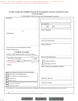


© Copyright 2026