
NYSERDA Home Performance with Energy Star Realization Rate
NYSERDA Home Performance with Energy Star Realization Rate Attribution Study Final Report Prepared for: New York State Energy Research and Development Authority Albany, NY Kim Lenihan Program Manager, Residential Energy Services Quality Standards and Compliance Prepared by: Performance Systems Development Ithaca, NY Jerone Gagliano VP, Energy Engineering Services Greg Thomas CEO NYSERDA Report HP-QA-04282014 NYSERDA Contract 32009 Revised January 2015 NOTICE This report was prepared by Performance Systems Development (PSD) in the course of performing work contracted for and sponsored by the New York State Energy Research and Development Authority (hereafter NYSERDA). The opinions expressed in this report do not necessarily reflect those of NYSERDA or the State of New York, and reference to any specific product, service, process, or method does not constitute an implied or expressed recommendation or endorsement of it. Further, NYSERDA, the State of New York, and the contractor make no warranties or representations, expressed or implied, as to the fitness for particular purpose or merchantability of any product, apparatus, or service, or the usefulness, completeness, or accuracy of any processes, methods, or other information contained, described, disclosed, or referred to in this report. NYSERDA, the State of New York, and the contractor make no representation that the use of any product, apparatus, process, method, or other information will not infringe privately owned rights and will assume no liability for any loss, injury, or damage resulting from, or occurring in connection with, the use of information contained, described, disclosed, or referred to in this report. NYSERDA Home Performance with ENERGY STAR Realization Rate Attribution Study i Abstract and Keywords This study, funded by the New York State Energy Research and Development Authority (NYSERDA) and performed by Performance Systems Development, identified the underlying causes for over-estimation of contractor-reported energy savings in the NYSERDA Home Performance with ENERGY STAR program for the years of 2007 to 2011 and assessed the potential impact on savings prediction accuracy of applying the ANSI/BPI2400 standard for baseline energy model calibration to actual energy usage. Whole building energy efficiency programs across the country have experienced shortfalls in the ratio of actual energy savings relative to contractor-reported savings when undergoing formal evaluation of savings results. This ratio of actual to contractor-reported savings is called the “realization rate”. The ANSI/BPI-2400 standard was developed based on best practices to provide energy efficiency incentive programs with a tool for improving the confidence in energy savings predictions from energy modeling tools when used as part of incentive approval in efficiency programs. This study tested the potential of the ANSI/BPI-2400 standard to improve prediction accuracy by retrospectively applying the standard to a group of over 2,000 homes retrofitted in the NYSERDA Home Performance with ENERGY STAR program over five years. The study also evaluated a wide range of other factors that could be contributing to reductions in project-level energy savings realization rates. The study found that: The most significant variable contributing to the relative accuracy of the savings predictions was the degree to which the baseline simulation model was calibrated to match the actual energy bills in the home. Programmatic application of the ANSI/BPI-2400 baseline energy model calibration standard will likely dramatically increase project-level realization rates (energy savings prediction accuracy). The medians of the contractor-reported percentage savings and the actual percentage savings were closely aligned, with the realization rate error being driven by a shortfall in the absolute value of the savings prediction resulting from the over-estimated baseline simulation models. The TREAT simulation software used by the program produced similar percentage savings estimates as compared with those from BEopt, a research-grade simulation tool from NREL and DOE’s Building America program. Other conclusions based on the findings in this study include: TREAT has been tested and accredited using the RESNET software verification tests for existing residential buildings. It is assumed that other energy simulation tools passing these RESNET software tests should produce similar results to the TREAT software when used in conjunction with the application of the ANSI/BPI-2400 standard. This could be validated through a future pilot study. The use of model calibration following the ANSI/BPI-2400 standard allows reduced detail in the energy models that undergo program review, reducing contractor effort and speeding up review time. These conclusions and others in the study are being used to help improve program realization rates, streamline program operations, and automate incentive approval. Keywords: NYSERDA, ANSI/BPI-2400, model calibration, realization rate, home performance, HPwES, program evaluation, TREAT, Green Button, automated desktop review, modeling software approval process NYSERDA Home Performance with ENERGY STAR Realization Rate Attribution Study ii Acknowledgements This report was prepared with support and assistance from Kimberly Lenihan, Karen Hamilton, and John Ahearn from NYSERDA’s Residential Energy Services Program as well as Dave Beaulieu from Conservation Services Group. NYSERDA Home Performance with ENERGY STAR Realization Rate Attribution Study iii Table of Contents NOTICE ...................................................................................................................................... i Abstract and Keywords ........................................................................................................... ii Acknowledgements .................................................................................................................iii Table of Contents .....................................................................................................................iv List of Appendices ..................................................................................................................vii List of Figures ........................................................................................................................viii List of Tables ............................................................................................................................ x Glossary of Terms and Acronyms ..........................................................................................xi 1 Executive Summary .......................................................................................................... 1 1.1 Overview ....................................................................................................................................... 1 1.2 Key Findings.................................................................................................................................. 2 1.1.1 Realization Rate Error Attribution .......................................................................................... 2 1.1.2 Model Calibration Addresses Most of the Error .................................................................... 3 1.1.3 TREAT Savings Predictions Algorithms ................................................................................ 4 1.3 2 1.1.4 Gradually Require Model Calibration .................................................................................... 4 1.1.5 Program Administrator Access to Utility Billing Data ............................................................ 5 1.1.6 Build in Automated Data Checks .......................................................................................... 5 1.1.7 Standardize Desktop Review ................................................................................................ 6 1.1.8 Enhance Field QA Process ................................................................................................... 6 1.1.9 Software Approval Process Enhancements .......................................................................... 6 1.1.10 Further Research Leveraging This Study ............................................................................. 7 Background ....................................................................................................................... 8 2.1 What is a realization rate? ............................................................................................................. 8 2.1.1 Why study realization rates? ................................................................................................. 8 2.1.2 What is baseline model calibration?...................................................................................... 9 2.2 3 Key Recommendations ................................................................................................................. 4 Testing the Hypothesis ................................................................................................................ 11 Attribution of Realization Rate Error ..............................................................................13 3.1 Differences in How Realization Rate were Determined for this Study ........................................ 13 3.2 Initial Significance Testing of Binary Factors .............................................................................. 14 3.3 Determining Attribution of Project-Level RR Error ...................................................................... 17 3.3.1 Investigate Preliminary Relationships between project-level RR and Predictor Variables . 17 3.3.2 Prediction Model to Explain the Project-Level RR Error ..................................................... 21 NYSERDA Home Performance with ENERGY STAR Realization Rate Attribution Study iv 3.4 4 5 3.4.1 Air Leakage Algorithm ......................................................................................................... 24 3.4.2 Surface Conduction Algorithms and Air Films .................................................................... 25 3.4.3 Domestic Hot Water Algorithms .......................................................................................... 26 3.4.4 Window Algorithms.............................................................................................................. 27 3.4.5 Comparison of Percentage Energy Savings Estimates ...................................................... 27 Potential Impact of Adopting ANSI/BPI-2400 Standard .................................................28 4.1 Model Calibration ........................................................................................................................ 28 4.2 Potential Impact on Contractor-Reported Savings and RR ........................................................ 29 Recommendations (QA and Program Policy) ................................................................32 5.1 Automated Checks and In-Model Feedback ............................................................................... 32 5.1.1 Verification of ANSI/BPI-2400 Standard Compliance ......................................................... 32 5.1.2 Standardize Desktop Review .............................................................................................. 33 5.1.3 Contractor-Reported Savings Threshold Check ................................................................. 33 5.1.4 Model Geometry Checks ..................................................................................................... 36 5.1.5 Additional Heating and Cooling Checks .............................................................................. 36 5.1.6 SIR Input Checks ................................................................................................................ 37 5.1.7 Improvement Input Checks ................................................................................................. 38 5.2 6 Investigating TREAT’s Savings Algorithms ................................................................................. 24 Improving Data Quality and Field QA ......................................................................................... 39 5.2.1 Targeting Field QA .............................................................................................................. 39 5.2.2 Improving Airsealing Savings Estimates ............................................................................. 39 5.2.3 Effective Insulation R-Values .............................................................................................. 40 Options for Energy Modeling Tool Approval .................................................................42 6.1 Comparison to Actual Building Data ........................................................................................... 42 6.2 Consultant Review ...................................................................................................................... 43 6.3 Building Physics Testing as done using RESNET Accreditation ................................................ 44 6.4 BESTEST-EX .............................................................................................................................. 46 6.5 Testing in General ....................................................................................................................... 46 6.5.1 Validation of User Inputs ..................................................................................................... 46 6.5.2 Improving Realization Rates and Accuracy ........................................................................ 46 6.5.3 Baseline Model Calibration ................................................................................................. 47 6.6 Software Testing Recommendations .......................................................................................... 48 6.6.1 Allow Two Tiers of Testing .................................................................................................. 48 6.6.2 Support Central Administration of Software Testing ........................................................... 48 6.6.3 Establish Dialog with NREL on Software Testing Options .................................................. 48 NYSERDA Home Performance with ENERGY STAR Realization Rate Attribution Study v 7 Market Transformation Impacts ......................................................................................49 7.1 Dataset Cleaning and Attrition .................................................................................................... 51 7.2 Attrition from Missing Data and Insufficient Billing Data Quality ................................................. 52 7.2.1 7.3 Attrition from Removing Outliers ......................................................................................... 52 Billing Data Regression Analysis ................................................................................................ 53 7.3.1 Billing Regression Analysis Using PRISM ......................................................................... 53 7.3.2 Calculation of the NAC ........................................................................................................ 54 7.4 Determining Significant Differences Among Factor Groups ....................................................... 54 7.5 Testing Normality of Key Variables ............................................................................................. 54 7.6 Determining Relative Attribution of Project-Level RR Error ........................................................ 55 7.7 Creating Synthetically Calibrated Model Savings ....................................................................... 55 NYSERDA Home Performance with ENERGY STAR Realization Rate Attribution Study vi List of Appendices Appendix A Documentation of Methodology ....................................................................51 Appendix B Dataset Characteristics..................................................................................56 Appendix C Summaries of Potential Impact of Implementing ANSI/BPI-2400 Standard68 NYSERDA Home Performance with ENERGY STAR Realization Rate Attribution Study vii List of Figures Figure 1: Energy savings predictions without calibration (left) and with calibration (right). .......................... 3 Figure 2: Baseline model compared to disaggregated pre-retrofit utility bills ............................................. 10 Figure 3: Impact of uncalibrated model on realization rates ....................................................................... 10 Figure 4: Impact of calibrated model on realization rates ........................................................................... 11 Figure 5: Natural gas correlations of predictor variables to RR .................................................................. 19 Figure 6: Electricity correlations of predictor variables to RR .................................................................... 20 Figure 7: Relative impact of 2007-2008 natural gas dataset with 95% confidence intervals shown on the bars. ............................................................................................................................................... 22 Figure 8: Relative impact of 2009-2011 natural gas dataset with 95% confidence intervals shown on the bars. ............................................................................................................................................... 22 Figure 9: Relative impact of 2007-2008 electricity dataset with 95% confidence intervals shown on the bars. ............................................................................................................................................... 23 Figure 10: Relative impact of 2009-2011 electricity dataset with 95% confidence intervals shown on the bars. ............................................................................................................................................... 23 Figure 11: These two charts of the 2007-2008 natural gas dataset show the difference in project-level RR with model calibration (right plot), and without (left plot). The black dashed line represents the ideal RR of 1.0 while the red line is the best linear fit through the data. ........................................ 28 Figure 12: These two charts of the 2009-2011 natural gas dataset show the difference in project-level RR with model calibration (right plot), and without (left plot). The black dashed line represents the ideal realization rate of 1.0 while the red line is the best linear fit through the data. ..................... 29 Figure 13: This plot shows the actual natural gas savings against the pre-retrofit natural gas usage from the 2009-2011 dataset. This relationship becomes the basis for the threshold on the contractorreported savings. The dashed red line represents one possible threshold, which could be made more or less conservative by adjusting the line to include all or a portion of the projects in the historical dataset. ........................................................................................................................... 34 Figure 14: This plot shows the contractor-reported natural gas savings against the same pre-retrofit natural gas usage intensity shown in the figure above. The dashed red line comes from the threshold established in the previous figure. ................................................................................. 35 Figure 15: This plot shows the adjusted (synthetically calibrated) contractor-reported natural savings against the same pre-retrofit natural gas usage intensity shown in the figure above. The dashed red line comes from the threshold established in the previous figure. This figure shows an example of how model calibration can eliminate much of the over-prediction of savings and save a lot of manual review time. ........................................................................................................... 35 Figure 16: This chart shows the impact of voids in insulation on the effective R-value for different nominal insulation R-values shown in the legend........................................................................................ 41 Figure 17: Actual and predicted natural gas pre-retrofit usage for 2007-2008 dataset .............................. 56 Figure 18: Actual and predicted natural gas pre-retrofit usage for 2009-2011 dataset .............................. 57 Figure 19: Actual and predicted electricity pre-retrofit usage for 2007-2008 dataset ................................. 57 Figure 20: Actual and predicted electricity pre-retrofit usage for 2009-2011 dataset ................................. 58 Figure 21: Actual and predicted natural gas savings for 2007-2008 dataset ............................................. 58 Figure 22: Actual and predicted natural gas savings for 2009-2011 dataset ............................................. 59 Figure 23: Actual and predicted electricity savings for 2007-2008 dataset ................................................ 59 Figure 24: Actual and predicted electricity savings for 2009-2011 dataset ................................................ 60 Figure 25: Project-level RR from 2007-2008 natural gas dataset. Dashed red line indicates 100% realization rate. ............................................................................................................................... 60 NYSERDA Home Performance with ENERGY STAR Realization Rate Attribution Study viii Figure 26: Project-level RR from 2009-2011 natural gas dataset. Dashed black line indicates 100% realization rate. ............................................................................................................................... 61 Figure 27: Project-level RR from 2007-2008 electricity dataset. Dashed black line indicates 100% realization rate. ............................................................................................................................... 61 Figure 28: Project-level RR from 2009-2011 electricity dataset. Dashed black line indicates 100% realization rate. ............................................................................................................................... 62 Figure 29: Reported percent infiltration reduction from 2007-2008 dataset. The red represents the median............................................................................................................................................ 62 Figure 30: Reported percent infiltration reduction from 2009-2011 dataset. The red represents the median............................................................................................................................................ 63 Figure 31: Correlation Diagram for 2007-2008 Natural Gas dataset. ......................................................... 64 Figure 32: Correlation diagram for 2009-2011 natural gas dataset. ........................................................... 65 Figure 33: Correlation diagram for 2007-2008 electricity dataset. .............................................................. 66 Figure 34: Correlation diagram for 2009-2011 electricity dataset. .............................................................. 67 Figure 35: ANSI/BPI-2400 process flow chart ............................................................................................ 80 NYSERDA Home Performance with ENERGY STAR Realization Rate Attribution Study ix List of Tables Table 1. This table first lists the proportion of project-level RR variance explained by the best fit regression model followed by the relative impact of each listed variable (all variables sum to 100%) on the variance explained. .................................................................................................... 3 Table 2 This table shows the contractor-reported savings and RR from this study along with the adjusted values and the percent change due to synthetic calibration of the baseline simulation models. .... 4 Table 3: Median realization rates by factor with significantly different group values for natural gas in both datasets. ......................................................................................................................................... 14 Table 4: Median realization rates by factor with significantly different group values for electricity in both datasets. ......................................................................................................................................... 16 Table 5: Testing of TREAT’s air leakage algorithms against BEopt ........................................................... 25 Table 6: Testing of TREAT's surface conduction algorithms against BEopt .............................................. 26 Table 7: Comparison of sample medians between reported to actual percentage savings estimates...... 27 Table 8: Summary of program contractor-reported savings and project-level RR along with the adjusted values to show the potential of adopting the ANSI/BPI-2400 standard ......................................... 30 Table 9: Ranges of energy cost rates found in the datasets ..................................................................... 38 Table 10: Summary of data attrition. The numbers in parentheses refer to the specific method(s) listed below this table. ............................................................................................................................. 52 Table 11: Summaries of the potential impact in contractor-reported savings and project-level RR if models were calibrated for 2007-2008 natural gas dataset. ...................................................................... 68 Table 12: Summaries of the potential impact in contractor-reported savings and project-level RR if models were calibrated for 2009-2011 natural gas dataset. ...................................................................... 71 Table 13: Summaries of the potential impact in contractor-reported savings and project-level RR if models were calibrated for 2007-2008 electricity dataset. ......................................................................... 74 Table 14: Summaries of the potential impact in contractor-reported savings and project-level RR if models were calibrated for 2009-2011 electricity dataset. ......................................................................... 77 NYSERDA Home Performance with ENERGY STAR Realization Rate Attribution Study x Glossary of Terms and Acronyms Normalized Annual Consumption (NAC) – The building annual energy consumption of a given year, usually separated by fuel type, in which the weather-dependent portion of the energy consumption has been normalized to represent typical weather. This allows an apples-to-apples comparison of the energy consumption from one period in time to another period as well as making future energy savings estimates that should be representative on average. Coefficient of Determination (R2) - Proportion of variability in a regression data set that can explained by the model. Non-Program Effects – Also referred to as Exogenous Effects. Any act that changes the energy consumption in a household that is not due to the energy saving measures installed through the energy efficiency program. Some common examples of this that occur after energy retrofit as compared to household before retrofit are: residents changing thermostat and/or water heater settings, change in number of residents, change in quantity of electric plugloads, remodeling the home, installing other energy-related upgrades that were not included in the scope of the retrofit that was part of energy efficiency program. Project-Level Realization Rate – This is to distinguish that the realization rates in this study were determined for each individual project and not across all project as is done for impact evaluations. See the beginning of Section 3 for a further explanation of the differences in how these project-level realizations were calculated and the reasons this was done. Adjusted Project-Level Realization Rate (Adj-PLRR) – Recalculating the project-level realization rates using the adjusted contractor-reported. These adjusted savings reflect the hypothetical case where the baseline simulation model used for calculating the savings estimates was perfectly calibrated to the weather-normalized savings analysis for the particular project. Contractor-Reported Savings – also referred to as Predicted Savings, Modeled Savings, and Estimated Savings. For this study, the contractor-reported energy savings came from the TREAT software. The savings estimates from TREAT are weather normalized to represent savings for typical weather for the project location. TREAT – The TREAT software is used by the majority of the participants in the NYSERDA Home Performance with ENERGY STAR program. TREAT runs the SUNREL physics engine for load calculations and provides tools such as comparisons of multiple scenarios, weather normalization of energy usage data, and the ability to align or “calibrate” the baseline model with the energy usage data. HPXML – Home Performance XML is a national data transfer standard for residential energy audit information. The TREAT XML exports used in this report were the foundation for this national standard. ANSI/BPI-2400 – This standard describes a methodology for the creation of a baseline model that is “calibrated” to normalized energy usage history of the building and includes boundary checks for inputs as well as a methodology for savings calculation relative to the baseline. NYSERDA Home Performance with ENERGY STAR Realization Rate Attribution Study xi CFM50 – A measurement of air leakage in cubic feet per minute using a blower door at a pressure difference of 50 Pascals between the inside and outside. SIR – Saving to Investment Ratio is a screening tool for savings relative to cost of installation over the life of a measure. NYSERDA Home Performance with ENERGY STAR Realization Rate Attribution Study xii 1 Executive Summary 1.1 Overview Many whole building programs are experiencing issues with realization rates, which are defined as the ratio of actual savings to contractor-reported savings. These adverse results are being determined through program evaluation and subsequently result in significant changes to calculated program cost-effectiveness; often many years after the installations were completed. This study attempts to uncover the underlying causes of the savings underperformance and offers program enhancement strategies to improve savings prediction accuracy. The specific objectives of the study are: To understand the key factors related to energy savings predictions that contribute to poor project-level realization rates through the analysis of actual billing and simulation model data To assess the impact of applying the ANSI/BPI-2400 standard programmatically to improve realization rates To evaluate how calculation algorithms in TREAT (the predominant modeling software used in the NYSERDA Home Performance with ENERGY STAR program during period covered by this study ) and other software tools could be affecting realization rates To recommend improvements to program process and quality assurance that could improve realization rates Two data sets were analyzed, one for the 2007 to 2008 program years and one for the 2009 to 2011 program years. The two data sets had similar characteristics and similar results. Whereas program impact evaluations often determine program savings from a fixed-effects regression model representing project factors across all projects, this study focused on investigating the sources of the realization rate error in the contractor-reported savings process. The unavailability of a control group for non-program effects or on installation quality and metrics also constrained investigation of broader effects. The study focused on determining project-level realization rates contrasting the contractor-reported savings against the normalized annual consumption (NAC) of the associated utility billing data using PRISM. This approach also allowed testing of the potential perproject accuracy impacts of the application of the ANSI/BPI 2400 energy model calibration standard to the simulation models developed by participating contractors. NYSERDA Home Performance with ENERGY STAR Realization Rate Attribution Study 1 Key Findings 1.2 The study found that: The most significant variable contributing to the relative accuracy of the savings predictions was the degree to which the baseline simulation model was calibrated to match the actual energy bills in the home. Programmatic application of the ANSI/BPI-2400 baseline energy model calibration standard will likely dramatically increase project-level realization rates (energy savings prediction accuracy). The medians of the contractor-reported percentage savings and the actual percentage savings were closely aligned, with the realization rate error being driven by a shortfall in the absolute value of the savings prediction resulting from the over-estimated baseline simulation models. TREAT produced similar percentage savings estimates as compared with those from BEopt, a researchgrade simulation tool from NREL and DOE’s Building America program. Other conclusions related to this study: TREAT has been tested and accredited using the RESNET software verification tests for existing residential buildings. It is assumed that other energy simulation tools passing these RESNET software tests should produce similar results to the TREAT software when used in conjunction with the application of the ANSI/BPI-2400 standard. This could be validated through a future pilot study that used real-time feedback on energy savings across a group of home performance contractors that were randomly assigned which energy modeling software to use on a given project. The use of model calibration following the ANSI/BPI-2400 standard forces the user to address inaccuracies in the baseline energy model regardless of the level of detail entered about the project. Therefore, model calibration allows for reduced detail in the baseline models that undergo program review thereby reducing contractor effort and speeding up review time. This energy balance approach is the process used in modeling commercial buildings. This cost saving approach could also be validated as part of pilot described above. These conclusions and others in the study are being used to help improve program realization rates, streamline program operations, and automate incentive approval. 1.1.1 Realization Rate Error Attribution The study identified a range of variables that correlated to poor realization rates. The most significant variables that explained the variation in realization rates are shown in the table below with their relative impact indicated as a percentage. These key variables and their relative impact came from best fit multivariate linear regression models. Even though the portion of realization rate variance explained by these regression models (one per dataset) are quite low (e.g. 18% for the 2007-2008 natural gas dataset), it should be understood that the listed variables and the regression models were only able to analyze the savings prediction portion of the realization rate variation as there was not supporting data on the installation quality/performance and no control group to normalize out non-program factors. Refer to Table 10 in Appendix A for the number of projects used in all analyses in this study. NYSERDA Home Performance with ENERGY STAR Realization Rate Attribution Study 2 Table 1. This table first lists the proportion of project-level RR variance explained by the best fit regression model followed by the relative impact of each listed variable (all variables sum to 100%) on the variance explained. Dataset Portion of project-level RR Variance Explained by the Regression Model Calibration Variance Infiltration Reduction Pre-Retrofit Air Leakage Pre-Retrofit EUI Cond Floor Area 2007-2008 Gas 18% 39% 54% 3% 4% N/A 2009-2011 Gas 11% 56% 30% 2% 12% N/A 2007-2008 Elec 16% 51% 4% 3% 35% 7% 2009-2011 Elec 18% 44% 7% 4% 38% 7% 1.1.2 Model Calibration Addresses Most of the Error The application of an ex-post (synthetic) calibration, such as the ANSI/BPI-2400 standard, to the datasets showed how the realization rates and the contractor-reported savings would have been adjusted if model calibration had been a requirement of the program. The results of this application of the standard improved the realization rates significantly with a corresponding reduction in the reported (predicted) savings for natural gas. This is in line with the hypothesis that un-calibrated models are typically over-predicting the baseline simulation model and therefore have over-predicted associated savings. The following figure shows the functional basis of the impact of baseline energy model calibration according the ANSI/BPI-2400 on the energy savings realization rate, shown as the X/Y ratio in the charts. Figure 1: Energy savings predictions without calibration (left) and with calibration (right). The table below shows that the average accuracy in savings predictions (i.e. realization rates) across both datasets was significantly increased while also reducing the contractor-reported savings as a result of the ex-post calibration. Additionally, there was a significant reduction in the variation in individual savings prediction accuracy. NYSERDA Home Performance with ENERGY STAR Realization Rate Attribution Study 3 Table 2 This table shows the contractor-reported savings and RR from this study along with the adjusted values and the percent change due to synthetic calibration of the baseline simulation models. Percent Change in Project-Level RR Resulting Due to Calibration Sum of Contract orReported Savings Sum of Adj Contract orReported Savings Percent Change in ContractorReported Savings Due to Calibration Total Projects in Study Median projectlevel RR Median Adj project -level RR 2007-2008 Gas (therms) 903 0.69 1.00 46% 312,366 201,075 -36% 2009-2011 Gas (therms) 1,241 0.63 0.86 37% 316,880 225,585 -29% 2007-2008 Elec (kWh) 482 1.65 1.40 -15% 508,190 535,295 5% 2009-2011 Elec (kWh) 572 3.18 2.84 -11% 336,673 390,675 16% Summary Across All Projects in Study 1.1.3 TREAT Savings Predictions Algorithms The TREAT energy simulation algorithms were reviewed as part of the study, focusing on areas that were identified as contributing to poor realization rates; insulation savings and air sealing savings. These areas of TREAT were in close alignment with the predictions from best-in-class modeling tools or differences were found to have minimal impacts. There issue of the accuracy of air sealing savings predictions from energy simulations tools in general has been identified as requiring further research. Further illustrating that the TREAT algorithms predict energy usage and savings well, the TREAT percentage savings predictions closely aligned with the actual percentage savings for the natural gas datasets; the contractorreported savings was 20.5% while actual savings was 19.4% for the 2007-2008 dataset, and 17.9% and 15.6% for the 2009-2011 dataset. The magnitude of the contractor-reported savings was off from the actual savings because the baseline simulation models were not calibrated to the baseline energy usage. 1.3 Key Recommendations 1.1.4 Gradually Require Model Calibration Since the application of a bound on pre-retrofit energy use based on the actual energy use of the building is such an effective method for trapping modeling errors as well as reducing the general tendency of models to over predict, the primary recommendation is to apply a simple energy end-use calibration, such as ANSI/BPI-2400, to an increasing range of projects. Options for gradually increasing the requirement of calibration could include: Projects with larger project cost Projects with deeper percentage energy savings NYSERDA Home Performance with ENERGY STAR Realization Rate Attribution Study 4 Access to accelerated or automated approval for loans An introductory requirement, for the first five projects for example, as a validation of user modeling ability A remedial measure on specific contractors selected for poor performance in some category including, potentially, actual measured realization rates. 1.1.5 Program Administrator Access to Utility Billing Data At the same time that calibration is being introduced, the infrastructure for improving access to utility bill data should be improved. The Green Button data transfer standard is relatively easy for utility to apply and reduces the cost of data entry. The Green Button Connect standard improves the ability of a utility customer to pass data directly to a program and/or contractor. Program Administrators benefit by enabling immediate verification of the pre-retrofit energy used based on the actual energy use of the home. The Green Button Connect standard has been successfully implemented in the California utilities and can help programs achieve other market transformation goals by better integrating actual energy usage into the retrofit process. 1.1.6 Build in Automated Data Checks The introduction of an HPXML standard (BPI-2100-S-2013 Standard for Home Performance-Related Data Transfer, developed with industry input including earlier TREAT XML output) has improved the ability to create automated software data quality verifications for submitted modeling results. Data quality checks can be of several types: Data input bounding (e.g. Input Constraints found in ANSI/BPI-2400) Internal cross verification (e.g. comparing ceiling area to floor area) Data output or results checking Data checks can occur in the software and be reported out as part of the modeling data submission (as in the TREAT XML) and/or data checks can occur in the program implementer’s systems after the model results are submitted to the Program Administrator by the modeler. Data checks in the software have the advantage of reducing the time to fix any issues and provide more training feedback to the modeler. Data checks at the time of submission to the implementation database can include checks not disclosed to the contractor and can better compare data across models. Simple extensions to the HPXML standard should be considered to support data quality assurance. Some of data checks recommended based on this study have already been included in the HPXML standard as a result of PSD’s participation in the working groups. Key data checks recommended in this study include: Apply Input Constraints (ANSI/BPI-2400) Verify the utility billing data quality (ANSI/BPI-2400) Verify or report verification of energy end-use calibration (ANSI/BPI-2400) Check for appropriate geometry Check heating and cooling equipment for appropriate sizing and efficiencies of installed equipment NYSERDA Home Performance with ENERGY STAR Realization Rate Attribution Study 5 Check SIR inputs Apply contractor-reported savings thresholds Cap the air sealing Btu savings per CFM50 reduction Verify test-in and test-out blower door test results are used in the air leakage savings calculation Verify that the effective assembly R-values of the insulation upgrades are used in the savings calculation There is Department of Energy funded research occurring to improve the ability to build quality assurance checks into energy simulations. Much of this activity is related to the OpenStudio development platform built on top of the EnergyPlus simulation. PSD is working with the National Renewable Energy Lab (NREL) to help deploy this technology and is NREL’s first national training partner for OpenStudio. 1.1.7 Standardize Desktop Review Software independent standards for the review of submitted energy models should be established. These standards should encourage the use of simplified modeling approaches. For example, simplified modeling approaches exist in TREAT but are not used widely due partly to early practices to modeling complex home geometries and current reviewer focus on TREAT’s complex modeling detail capability. Model detail in more complex software tools should be an option and not a requirement, unless there is a specific and pre-established need for using that level of detail. Once standards for model review exist, both modelers and reviewers can be trained in that standard. 1.1.8 Enhance Field QA Process The study identified key areas where post installation quality assurance could impact realization rates. These include: Establish a grading system for insulation voids to obtain effective post-retrofit assembly R-values Increase QA of data inputs with greater savings impact, such as air leakage measurements Targeting contractors with historically lower realization rates for greater QA It is important that the QA process not create feedback on variations between the model and reality that are not significant to contractor-reported savings. Simplification of the modeling process will create more variation between the model and the real building. QA inspectors will need training and perhaps the ability to quickly remodel the building in a simple tool to be able to determine if a simplified model was simplified successfully or if the contractor needs feedback on elements of the model that are producing significant savings error. 1.1.9 Software Approval Process Enhancements As the range of tools diversifies and simplified models are introduced, it will be important to have screening methods for results as well as minimum feature requirements of the software tools (e.g. HPXML output, supports calibration). Methods for approval of software in programs should be a national effort, similar to the effort supporting HPXML and for similar reasons. Coordination with and support of these national efforts will best NYSERDA Home Performance with ENERGY STAR Realization Rate Attribution Study 6 support state and program level needs while allowing software vendors to focus resources on product improvement instead of testing state-by-state. 1.1.10 Further Research Leveraging This Study Considerable effort has been undertaken to process the data sets and put them into a framework that can be readily queried. While undertaking this research effort additional research has been identified that could leverage the existing data sets. Establish cap on air sealing savings predictions – Work with the data to empirically determine a Btu savings per CFM50 that would reduce the current negative impact of air sealing on the realization rate. Test efficient QA methods such as parametric modeling – Test the application of percentage savings from sample simulations to the actual billing data to produce a quick savings check on the models that are being reviewed. Air sealing was determined to be a specific area for calculation improvement identified in the study. Support for empirical research on improving air sealing calculations is a key to improving the predictive ability of residential energy modeling software. In the interim, methods for limiting predicted air sealing savings should be considered. NYSERDA Home Performance with ENERGY STAR Realization Rate Attribution Study 7 2 Background 2.1 What is a realization rate? Realization rates are typically calculated as the ratio of the contractor-reported savings to the determined actual savings. A realization rate of less than 1.0 (or less than 100%) means that the actual savings are less than predicted, this is usually referred to as a savings shortfall. A realization rate of greater than 1.0 (more than 100%) means that the savings are greater than predicted. Realization rates of greater than 1.0 are not common. 2.1.1 Why study realization rates? Since the program realization rates are typically calculated by program evaluators several years after the actual installations were completed, the evaluator adjustments (usually lower) to savings predictions are applied after the program funds have been spent. This ex-post savings adjustment can lead to failed cost-effectiveness tests, increasing the risk of program cancellation. Realization rates have been a major issue for whole-building energy efficiency programs in part because these programs have tended to be less cost-effective than simpler rebate programs, often operating at or near cost-effectiveness thresholds. Shifting from whole-building energy savings calculations to deemed savings is one solution to reduce the risk of savings shortfall at time of evaluation. Deemed savings approaches intrinsically better align savings prediction with program evaluation. But the limitation of deemed savings calculations can have significant impacts on the delivery of whole-building savings approaches including failure to account for interactivity between measures. Deemed savings calculation approaches also tend to be associated with measure level cost-effectiveness screening, increasing the problems that contractors have in aligning project workscope with the combination of energy and non-energy benefits sought by their customers. In order to meet the goal of improving cost-effectiveness, it is also important to reduce program operating costs, for both the program administrator and the participating contractors. Simplification of energy modeling as enabled by model calibration can reduce contractor costs associated with program participation. Additionally, standardization of energy model quality assurance by program administrators can provide significant cost savings as well. Better understanding of how to improve realization rates in a timely and cost-effective manner will have a positive effect on whole-building energy efficiency programs nationally. Expedited feedback on realization rates from proposed tools such as Efficiency Meters will allow whole-building programs to adjust modeling strategies midstream to cost-effectively meet savings goals. NYSERDA Home Performance with ENERGY STAR Realization Rate Attribution Study 8 2.1.2 What is baseline model calibration? Baseline models are energy simulation models that represent the actual pre-retrofit performance of a building. These models are then adjusted to represent the installation proposed improvements to energy use. Predicted savings are the fundamental difference between an improved model and a baseline model. A calibrated baseline model aligns actual pre-retrofit energy use with modeled energy use, as in Figure 2 below. Since most energy models use standard normalized weather files and not actual weather, the pre-retrofit energy bills are typically normalized to allow the calibration. Realization rate errors can be thought of consisting of two primary components: 1. 2. The error between the actual pre-retrofit energy consumption and the baseline energy model The error between the actual post-retrofit energy consumption and the post-retrofit performance prediction from the energy model. The technique of baseline simulation model calibration focuses on directly improving the first component and indirectly improving the second component. One baseline model calibration approach has been described in the ANSI/BPI-2400 standard. This approach requires the user of the energy modeling software tool to produce a baseline simulation model whose performance does not exceed the disaggregated actual energy use, see the flow chart in Appendix C for an overview of the process. As part of the energy usage normalization process, the usage is split up into components that are responsive to cold temperatures, to warm temperatures, and not responsive to temperature at all. Matching the baseline model to these end uses is assumed to reduce over prediction of savings. Testing this assumption is one of the goals of this study. Figures 2 and 3 below visually depict the impact that an uncalibrated baseline simulation model can have on contractor-reported savings and realization rate compared to a calibrated model. The ANSI/BPI-2400 standard was originally developed to help support a national tax credit based on saving predictions. The ANSI/BPI-2400 standard was designed to help prevent tax fraud by reducing the incidence of inflated energy savings. The standard relies on independently verifiable historical energy usage to prevent the inflation of pre-retrofit energy usage. NYSERDA Home Performance with ENERGY STAR Realization Rate Attribution Study 9 Figure 2: Baseline model compared to disaggregated pre-retrofit utility bills Figure 3: Impact of uncalibrated model on realization rates NYSERDA Home Performance with ENERGY STAR Realization Rate Attribution Study 10 Figure 4: Impact of calibrated model on realization rates 2.2 Testing the Hypothesis A range of hypotheses related to the modeled savings estimates have been put forward to explain realization rate short-falls in whole-building retrofit programs. They include: Improper use of modeling tools. Some examples are: o o o Users exaggerate performance failures of the existing building components (e.g. walls entered as uninsulated when they actually have some insulation, AFUE of existing furnace entered much lower than combustion efficiency because equipment is old) Users enter the home’s thermostat settings into the model, however, thermostat settings in energy models represent a uniform temperature for the entire model zone (typically the whole house in Home Performance programs), which is typically not the case in poor performing homes. Users select a surface (e.g. ceiling, wall) from the modeling tool library has the same description as the nominal insulation they propose to install, however, the post-retrofit insulated surface condition described in the model is uniformly insulated and this is often not the case even with a quality installation. Modeling tool calculation standards do not yield calculations that align with actual performance of energy conservation measures. Both examples below can contribute the observation that new construction modeling predictions tend to be more reliable than predictions for pre-retrofit existing buildings.1 o Air leakage calculations are not validated and could use additional research 1 Appendix A of http://www.nrel.gov/docs/fy11osti/50865.pdf http://www.resnet.us/blog/wp-content/uploads/2012/08/Houston-Energy-Efficiency-Study-2009-Final.pdf NYSERDA Home Performance with ENERGY STAR Realization Rate Attribution Study 11 o Insulation performance can be affected by air leakage in pre-retrofit and post-retrofit buildings. These effects may not be accounted for in wall R-values assumed by the software or the software user. Deliberate inflation of energy savings to gain access to program incentives NYSERDA Home Performance with ENERGY STAR Realization Rate Attribution Study 12 3 Attribution of Realization Rate Error There are many reasons for program realization rate error. As realization rate is the ratio of contractor-reported savings (estimated savings) to determined savings (actual savings), the sources of error in the contractor-reported savings can include simulation software error, user input error and/or exaggerations to increase contractor-reported savings, field data collection and measurement error. The sources of error in the determined savings can include poor retrofit installation quality, poor billing data quality, methods used for weather normalization of the billing data, and non-program effects (e.g. changes in home energy use not due to the retrofit such as change in occupancy). Whereas third-party program impact evaluations often determine program savings from a fixed-effects regression model representing project factors across all projects, this study focused on investigating the sources of the error in the contractor-reported savings portion of the realization rate. The lack of an available control group for nonprogram effects or on installation quality and metrics constrained investigation of broader effects. This study determined project-level realization rates from evaluating the contractor-reported savings and the normalized annual consumption (NAC) of the associated utility billing data using PRISM in order to test the per project impacts of the application of the ANSI/BPI 2400 standard to the simulation models developed by participating contractors. The goal of this study was to determine the variables that have the biggest impact on project-level RR, and to the extent possible, account for their relative portion of the project-level RR error. This section describes the specific effort completed in this study to assess impact of the following elements: Explain how project-level RR was determined for this study as compared to methods used in program impact evaluations. Explore the differences of project-level RR among program-related groups (e.g. assisted home performance projects, market rate projects, etc.) Investigate the key variables that most significantly account for project-level RR error Investigate and cross-validate the algorithms in TREAT used for calculating savings related to building envelope (e.g. insulation and air sealing) upgrades and domestic hot water. 3.1 Differences in How Realization Rate were Determined for this Study As this study is focused on explaining sources of error in the savings predictions, the methods used for determining the realization rates (RR) are different from those used in the program impact evaluation and therefore are not equivalent or comparable. While the details of the methodology can be found in Appendix A, it is useful to understand some of major differences in how realization rates were determined for this study. Determination of project-level actual savings and RR were not corrected for non-program effects (no control group data were available). NYSERDA Home Performance with ENERGY STAR Realization Rate Attribution Study 13 3.2 To investigate the effect of individual savings prediction factors (e.g. accuracy of the audit software, software input errors, etc.), this study calculated the actual savings and realization rate for each individual project. Typical impact evaluations determine a realization rate for contractor-reported savings across all projects using a fixed-effects regression model of the utility billing data and relevant project factors. To give an apples-to-apples comparison between actual and contractor-reported savings, this study determined the normalized annual consumption (NAC) for both the pre- and post-retrofit utility billing data using the same TMY2 (typical meteorological year from 1961 through 1990) average weather data that was assumed to have been used in the simulation models. The weather station selected was based on zip code as the station name was not part of the model export file. TMY2 files were used instead of the newer TMY3 since most of the simulation models were created before TREAT incorporated the newer TMY3 weather files in 2010. In contrast, the impact evaluation of the 2007-2008 NY State Home Performance program, used the average weather from 2003 through 2009 to determine the weather normalized actual savings to compare to the contractor-reported savings for determining the program RR. The use of 2003 through 2009 weather data instead of the same weather data that the simulation models used (TMY2) results in an average 5.6% error for 2007-2008 dataset, which means that even if the TREAT model predictions were completely without error, the TREAT contractor-reported savings would still be 5.6% higher than the evaluated “actual savings," thereby reducing the realization rates. Initial Significance Testing of Binary Factors Before examining which variables best account for project-level RR error, it is helpful to look at how project-level RR varies between the different levels of key program factors. For clarification, factors can be thought of as categories such as heating system equipment type, project location, or field QA inspection. Many factors were tested for whether or not there was a significant difference in median project-level RR between the binary state (e.g. yes/no) of each factor. Only those found to be significantly different are presented in the tables below. Because home performance retrofits tend to be multiple measure and whole house upgrades, none of the factors tested were isolated and therefore are not independent of the other factors tested. Refer to Table 10 in Appendix A for the number of projects used in all analyses in this study. Table 3: Median realization rates by factor with significantly different group values for natural gas in both datasets. Median Realization Rates by Factor Binary factors with significantly different realization rates Gas 2007-2008 Gas 2009-2011 Yes No Yes No Assisted Home Performance 54% 79% no data no data Field QC Inspection 60% 71% no data no data Pass ANSI/BPI-2400 Calibration Criteria 122% 66% 91% 61% Model Heating System Size is Sufficient 80% 52% 67% 43% Project Has Airsealing Improvement 61% 109% 51% 71% Project Has Insulation Improvement 72% 114% 59% 70% Project Has Heating Improvement 62% 72% 59% 72% Project Has Window Improvement 89% 62% 108% 58% Project Has More Than One Gas Improvement 66% 163% 61% 117% NYSERDA Home Performance with ENERGY STAR Realization Rate Attribution Study 14 These factors do not in and of themselves explain project-level RR error but may help guide the analysis into the attribution of error in realization rates as well as highlight places in the program that may need to be reexamined such as file review and field QA. Some additional investigation was performed for each of the factors listed in the table above to try to understand the reason for the difference in project-level RR. The hypotheses for the differences in project-level RR among factors are listed below for both program years as well as differences between program years. Affordable vs Market Rate – there are several reasons why the project-level RR could be lower for Affordable Home Performance projects. The most likely reason is the large incentive that requires an SIR greater than 1.0 tends to bias contractors to model the home’s existing performance worse than it really is in order to increase the contractor-reported savings. Additionally, there may be some “take back” effect (e.g. using more because the owner can now afford to keep the home warmer, for example) for both program years as the natural gas prices in NY State have fallen from 2008 through 2012, but this is likely a secondary reason. Field QC Inspection – it is not fully understood why the project-level RR are significantly better for the projects that did not receive a field QC inspection but likely due to confounding by other factors in the table above that negatively impacted project-level RR. Comparing the two groups, field QC vs. no field QC, the data showed that the field QC group had a higher percentages of affordable projects, projects with airsealing, projects with insulation, and projects with more than one improvement, all factors that had lower project-level RR. Passing the ANSI/BPI-2400 Calibration Criteria – this clearly shows a very strong correlation between calibrating the baseline simulation model and realizing the estimated savings. In the 2007-2008 dataset there were 48 projects with models that met the calibration criteria and 89 projects in the 2009-2011 dataset. The reason for this large difference in project-level RR is because calibrating the baseline model greatly reduces over-prediction of the savings estimates as they become ‘scaled’ by the baseline utility bill history. Model Heating System Size is Sufficient – the system size not being sufficient happens one of two ways, sometimes as an input error leaving off a zero or most often as the result of an uncalibrated baseline model inputs that result in an inflated heating load too large for the entered heating equipment capacity. The undersized heating equipment is similar to a threshold of lack of baseline model calibration. If the model is uncalibrated far enough that the heating load exceeds the heating equipment capacity, then these models have a good chance of being some of poorest calibrated models and therefore will have overestimated savings predictions and poor project-level RR. Projects with Insulation Improvements – this can likely be attributed to incorrectly entering the effective insulation value of the installed insulation into the TREAT model because voids were not accounted for. This issue has been explored further in Sections 3.4 and 5.2. Projects with Airsealing Improvements – the primary reason is likely due to simulation models (TREAT, REM/Rate, EnergyPlus, etc.) not accounting for the complex and dynamic relationship in heat loss/gain between air exchange and that of the surfaces of the conditioned space and interstitial spaces (e.g. inside of walls, floor between stories) as well as buffered zones (e.g. attics and unconditioned basements and crawlspaces). This issue has been explored further in Sections 3.4 and 5.2. Project has Heating Improvement – the likely reason for this is not accounting for the real world efficiency of the new equipment being installed. Most contractors enter the rated AFUE into the TREAT improvement; however, these efficiencies are rarely achieved in a retrofit unless the new equipment was paired with new and properly sized distribution system. The new furnace will run longer resulting in a drop in actual AFUE if the distribution system was not improved and supplies/returns are still covered with furniture. The new condensing boiler will run longer resulting in a drop in actual AFUE when NYSERDA Home Performance with ENERGY STAR Realization Rate Attribution Study 15 installed using the existing hydronic distribution that was designed for high temperature water. These issues lead to unintentional over-predictions of the post-retrofit performance and therefore lower projectlevel RR. Project Has Window Improvement & Project Has More Than One Gas Improvement – these are listed together because the data show that they are interrelated. For 2007-2008 dataset, 78% of the single gas measure projects were window installations and this set contains about a third of the projects that passed the ANSI/BPI-2400 calibration criteria. For the 2009-2011 dataset, 50% of the single gas measure projects were window installations. The reason window improvements are showing such high projectlevel RR is likely because the contractor-reported savings from TREAT are being underestimated (more conservative). One of the possible reasons for this is that the contractor only entered the improvement to the window’s U-value performance and did not add an airsealing measure to capture the reduced air leakage around the old windows. Modeling tools separate out the effects of air sealing which is a whole building improvement from surface area improvements such as windows and insulation. Window surface improvements occurring without an accompanying air sealing measure is a strong indication that the user needed training. Refer to Section 3.4 regarding accuracy testing of TREAT’s algorithms for window savings. Table 4: Median realization rates by factor with significantly different group values for electricity in both datasets. Binary factors with significantly different realization rates Median Realization Rates by Factor Electricity 2007-2008 Electricity 2009-2011 Yes No Yes No Assisted Home Performance 117% 210% no data no data Project Has Cooling Equipment Improvement 227% 153% 411% 245% Project Has Airsealing Improvement not sig not sig 226% 362% Project Has Insulation Improvement not sig not sig 236% 363% Project Has More Than One Electric Improvement 67% 147% not sig not sig Project Has Lighting Improvement 136% 284% 112% 397% Project Has Appliance Improvement 120% 182% 110% 440% Almost all of the median values of the electricity project-level RR shown above are all greater than 100% which is very different from the program-level RR of about 35% determined in the Home Performance with Energy Star 2007-2008 Impact Evaluation report. As stated in Section 3.1, the project-level RR were calculated very differently than the methods used by impact evaluations and the purpose of reporting the median of the project-level RR was for making comparisons and understanding attribution of error. For more information on the data cleaning that was performed and how this may or may not have impacted the resulting project-level RR, see Appendix A and Section 4.2. Even though almost all of the median project-level RR in the table above are over 100%, the emphasis here is that there is still a significant difference between the Yes and No categories. Assisted Home Performance – the reasons for the difference would be the same as listed above for the natural gas datasets NYSERDA Home Performance with ENERGY STAR Realization Rate Attribution Study 16 3.3 Project Has Cooling Equipment Improvement – these improvements tended to double the median projectlevel RR meaning that these improvements saved more than was predicted by the TREAT models. This suggests that the TREAT modeled cooling savings were under-estimated as compared to the actual savings. This could be due to the TREAT cooling algorithms and/or model inputs. For instance, it was found that about 25% of projects in the 2007-2008 dataset and 50% of the projects in the 2009-2011 dataset that installed new AC equipment used SEER 10 or greater as their input for the existing AC equipment efficiency. These SEER might be too conservative and were likely based on the nameplate data not taking into account the actual in-situ efficiency of the equipment that would be lower (e.g. improper airflow, refrigerant charge). Project Has Airsealing Improvement – the reasons for the difference in the 2009-2011 dataset would be the same as listed above for the natural gas datasets. The likely reason there is a significant difference in the 2009-2011 but not the 2007-2008 dataset is because 88% of the projects modeled cooling in the baseline simulation model in the 2009-2011 dataset while 46% in the 2007-2008 dataset. Both datasets only had about 4% of projects with electric heating. Modeled electricity savings from this improvement only showed up if electricity was being used for heating and/or cooling. Project Has Insulation Improvement – same reasoning as for Project Has Airsealing Improvement Project Has Lighting Improvement – the likely reason for the difference is due to user input assumptions for hours the lights are on and/or the wattage reduction. TREAT does account for the interaction of the reduced internal heat gains from the lighting wattage reduction on the heating and cooling systems. See the Improvement Input Checks portion of the Recommendations section. Project Has Appliance Improvement – similar reasoning as for Project Has Lighting Improvement. The most common electric appliance upgrade is a new refrigerator and the likely source of error is the assumption of the annual electricity usage of the existing refrigerator. Determining Attribution of Project-Level RR Error The primary goal of this study was to determine which variable(s) best explain all or some of the project-level RR error. This attribution of error took the form of a multivariate linear regression model of project-level RR as a function of one or more predictor variables. Once the best regression model was determined and validated, a technique was used to apportion the relative amount of variance in project-level RR explained by each predictor variable. In the previous section, differences in project-level RR between program factors were explored and large differences were found in project-level RR between projects that passed the ANSI/BPI-2400 calibration criteria and those that did not, and projects that included an airsealing improvement. These relationships are further explored in the section below along with other predictor variables. 3.3.1 Investigate Preliminary Relationships between project-level RR and Predictor Variables To help determine which predictor variables are most correlated to the response variable, project-level RR variation, correlation diagrams were generated, as shown in Figures 31 through 34 in Appendix B. The diagrams indicate the sign of the correlation between two variables and the magnitude of correlation. To simplify the correlations in the diagram to focus only on that of project-level RR, the correlation values between each predictor variable and project-level RR were compiled in bar charts below. The scope of the study was constrained to primarily investigate NYSERDA Home Performance with ENERGY STAR Realization Rate Attribution Study 17 areas of over-prediction in the simulation models as NYSERDA was interested in explaining the low project-level RR from the impact evaluation reports. The study investigated variables with a significant signal (e.g. Calibration Var, dACH%). Initial testing found that contractor-reported savings from AC equipment and window upgrades appeared to be under-predicting because of the project-level RR were over 100%. However, there were only a small number of projects with this finding and the majority of them were related to only a few specific contractors. Refer to Table 10 in Appendix A for the number of projects used in all analyses in this study. Definitions of variables in the correlation bar charts: Infiltration Reduction – percentage infiltration reduction as reported in the TREAT model from the base building blower door number and the reported Test-Out blower door number Pre-Retrofit Air Leakage – air changes per hour at 50 pascals pressure difference as measured at the TestIn blower door Heating Equip Eff – the seasonal efficiency of the existing primary heating equipment as entered by the contractor into the TREAT model Calibration Variance, Total – the calibration variance of all end-uses (heating, cooling, and baseload) for the fuel type. Calculated as the difference in the weather normalized annual usage between the baseline TREAT model and the pre-retrofit bills divided by that of the pre-retrofit bills Calibration Variance, Heating – the calibration variance of the heating end-use for the fuel type Calibration Variance, Cooling – the calibration variance of the cooling end-use for the fuel type Calibration Variance, Baseload – the calibration variance of the baseload end-use for the fuel type Cond Floor Area – the area of all conditioned spaces as entered by the contractor into the TREAT model Year Built – year home was built from the program implementer’s database) Pre-Retrofit EUI – the pre-retrofit weather normalized energy usage intensity for the fuel type in units of kBtu/Sq.Ft. NYSERDA Home Performance with ENERGY STAR Realization Rate Attribution Study 18 Figure 5: Natural gas correlations of predictor variables to RR The relationship of the predictor variables to project-level RR was used to test out different multivariate linear regression models in the next section. The following conclusions were drawn from the correlation matrix for both 2007-2008 and 2009-2011 natural gas datasets, differences are noted where they exist. The correlation percentages (bars) for the two program datasets are very similar, which implies that there are underlying issues that are responsible for project-level RR errors beyond programmatic changes (e.g processes/requirements) and contractor participation. The largest correlation with natural gas project-level RR error is Total Calibration Variance. While the total model calibration variance could be used, the calibration variance by heating and baseload end-uses are more useful in the program in order to comply with ANSI/BPI-2400 and ensure that savings predictions by measure are more accurate. For example, the baseline simulation model could be calibrated on a total annual usage basis, but this may have been done suppressing the inputs for domestic hot water in order to shift gas usage from baseload to heating end-use thereby making the heating related improvements more cost-effective. The next largest correlation was Infiltration Reduction though it is larger for the older 2007-2008 dataset than the 2009-2011 dataset. This is likely because 22% of the program reported natural gas savings from air sealing improvements in the 2007-2008 dataset versus 15% in the 2009-2011 dataset. Additionally, other studies have shown that modeled air sealing savings over-predict actual savings due to dynamic and NYSERDA Home Performance with ENERGY STAR Realization Rate Attribution Study 19 complex heat loss/gain, which further explains the large and negative correlation. The ACH50 (Test-In Blower Door number) is related to this as well. Heating Equip Efficiency has a small positive correlation with project-level RR for the 2009-2011 dataset while it does not exist for the 2007-2008 dataset. Conditioned Floor Area has a small negative correlation with project-level RR for the 2007-2008 dataset and none for the 2009-2011 dataset. Floor area should not impact project-level RR directly, however, larger homes tend to be more complex and have more floors and additions and it is possible that the auditors tried to model all of these complexities when they should have used a single zone/space model. Year Built has a small positive correlation to project-level RR for the 2007-2008 dataset and none for the 2009-2011 dataset. In general, the newer homes should behave more like simulation models because things like exterior walls are fully insulated as opposed to the mix of uninsulated and partially insulated walls often found in older homes. Analyzing the distributions of the age of homes between the two datasets, 15% were built in 1980 or newer in the 2007-2008 dataset, while the 2009-2011 dataset had 29% built in 1980 or newer. Pre-Retrofit EUI exhibits similar positive correlation with project-level RR for both datasets. The likely reason for this is that the more energy intensive homes coincidently align better with uncalibrated simulation models and there is more potential savings in these homes so the savings signal to annual usage noise is lower. Figure 6: Electricity correlations of predictor variables to RR NYSERDA Home Performance with ENERGY STAR Realization Rate Attribution Study 20 The following conclusions were drawn from the correlation matrix for both 2007-2008 and 2009-2011 electricity datasets, differences are noted where they exist. The most significant correlation is that of the Total Calibration Variance and it appears that this can mostly be attributed to the Cooling Calibration Variance. This is logical because cooling savings in a retrofit scale with the baseline cooling energy consumption, whereas savings from lighting, for example, does not scale with baseload energy consumption because savings are more dependent on hours of operation. One of the only real differences between the two datasets in the figure above is that of Baseload Calibration Variance. This could be due to modeling practices changed between program years. The second most significant correlation is that of the Pre-Retrofit EUI, which is positive. The more electricity usage intensive the home is, the more potential there is for savings. The Cond Floor Area has a small positive correlation, which is likely explained by the amount of electric baseload that scales with the floor area (lighting is the main electric improvement that scales with floor area). The Year Built has a small positive correlation likely for the same reason as above in the natural gas datasets; newer homes behave more like simulation models. Both the Infiltration Reduction and Pre-Retrofit Air Leakage variables had little correlation to electricity project-level RR since very few homes had electric heating systems and cooling energy consumption is low in the climate. 3.3.2 Prediction Model to Explain the Project-Level RR Error As discussed in the beginning of this section, this study was focused on exploring the attribution of error in the savings predictions from individual projects. The figures below show the relative contribution of each significant predictor variable on project-level RR error as the percentage of the R2, which is the proportion of variance explained by the regression model. As can be seen from the R2 listed at the bottom of each figure, the proportion of variance in project-level RR explained by these models was quite low. This is reasonable as this study does not take non-program effects into account or installation quality. The takeaway is the relative contribution or importance of each of the predictor variables. The relative contributions should be used to help guide decisions around which aspects of the program should be changed. Presented below are four charts broken out by program year and fuel type. Refer to Table 10 in Appendix A for the number of projects used in all analyses in this study. NYSERDA Home Performance with ENERGY STAR Realization Rate Attribution Study 21 Figure 7: Relative impact of 2007-2008 natural gas dataset with 95% confidence intervals shown on the bars. Figure 8: Relative impact of 2009-2011 natural gas dataset with 95% confidence intervals shown on the bars. NYSERDA Home Performance with ENERGY STAR Realization Rate Attribution Study 22 Figure 9: Relative impact of 2007-2008 electricity dataset with 95% confidence intervals shown on the bars. Figure 10: Relative impact of 2009-2011 electricity dataset with 95% confidence intervals shown on the bars. NYSERDA Home Performance with ENERGY STAR Realization Rate Attribution Study 23 3.4 Investigating TREAT’s Savings Algorithms In an effort to assess whether or not the TREAT software is a potential source of error in the contractor-reported savings, several comparisons were carried out to cross-validate TREAT’s savings algorithms. In the sections below, TREAT savings for air leakage reductions, surface insulation, and windows are compared with those from researchgrade modeling software. Additionally, the contractor-reported savings are compared to the actual savings on a percentage basis. 3.4.1 Air Leakage Algorithm Before the air leakage algorithms were tested in TREAT, the pre- and post-retrofit infiltration numbers used in the projects with airsealing improvements were investigated to see if they were reflective of the real Test-In and TestOut blower door numbers. An issue with airsealing is that savings are sometimes based on a contractor’s educated guess on how much he/she will be able to reduce the air leakage in a home which is submitted as the CFM50 improvement in TREAT. This is usually done by assuming a 20% or 30% reduction of the CFM50 used in the base model, which should come from the Test-In number. TREAT has a section that records the BPI health and safety measurements as well as blower door numbers, but the blower door values are not required so only a small portion of the models with airsealing improvement had both a Test-In and Test-Out blower numbers recorded in the Measurements section of TREAT. A simple technique was used to detect if airsealing improvement savings were based on the final Test-Out blower door number or the best guess of a contractor. By looking at the percentage air leakage reduction values, those values with a long string of decimal places (as would be expected dividing two random numbers) were representative of airsealing savings based on Test-Out blower door numbers, whereas values with three or less decimal places (eg 0.305) were representative of airsealing savings based on a percent reduction estimate. It was assumed that contractors did not choose a random blower door number for the proposed airsealing improvement. With this technique, it was determined that 4% of the airsealing projects had not updated the best guess value with Test-Out blower door number for the 2007-2008 dataset, and 1% for the 2009-2011 dataset. While all airsealing savings should be based on the difference between Test-In and Test-Out blower door numbers, this small percentage does not explain the significant difference in project-level RR that is shown in the Initial Significance Testing of Binary Factors section above. Since the testing of blower door inputs above showed only a small percentage of contractors who did not update their final model submission with the test-out blower door value, over-prediction of savings from airsealing may be due to the TREAT algorithms for air leakage. The TREAT air leakage algorithms have not changed since 2007 and TREAT has passed the Building Energy Simulation Tests (BESTEST) which parallels ANSI/ASHRAE Standard 140-2001 Standard Method of Test for the Evaluation of Building Energy Analysis Computer Programs. These tests stress the limits of the simulation models to predict heating and cooling energy for extremely high and low air leakage rates. To investigate this further, PSD cross-validated the contractor-reported savings from air leakage NYSERDA Home Performance with ENERGY STAR Realization Rate Attribution Study 24 reduction improvements against BEopt, NREL and DOE’s Building America program research-grade residential modeling tool (http://beopt.nrel.gov) which runs on EnergyPlus (the leading simulation engine). The crossvalidation tests were performed using a simple single-story residential home located in Syracuse, NY with a standard pitched roof attic and two different foundation types. All models tested in TREAT and BEopt had the same envelope characteristics, internal gains, thermostat set points, and HVAC equipment input. Three different degrees of air leakage reduction were tested in both models. The results of the cross-validation test shown in the table below produce very similar estimated savings as a percentage of the modeled heating and cooling energy use. These results are expected as TREAT passes the BESTEST test suite, and in all cases, TREAT predicted less savings than BEopt. Table 5: Testing of TREAT’s air leakage algorithms against BEopt Percentage Savings of Heating and Cooling Energy Slab-on-grade Unconditioned Basement 20% air leakage reduction 40% air leakage reduction 60% air leakage reduction BEopt 9% 18% 27% TREAT 7% 14% 22% BEopt 9% 17% 25% TREAT 8% 15% 23% With TREAT air leakage algorithms validated as compared to other simulation tools, the logical conclusion is that some simulation tools are making assumptions that do not account fully for the heat that is lost/gained from air infiltration/exfiltration. In fact, this is the subject of an ongoing debate in the building science community, and there is growing evidence that supports this theory. The issue is that heat loss due to air leakage is much more complex and dynamic than even EnergyPlus is accounting for. The current hypothesis among industry leaders is that infiltrating air into the basement or crawlspace picks up heat loss in that space (and duct losses if present) and brings that into conditioned space. Leaking air to the attic warms the attic which reduces the temperature difference across the attic floor insulation and therefore reduces the actual heat loss. Some presentations at home performance conferences have suggested that actual savings from airsealing are about 40% less than the predictions from the simulation models. See Section 5.2.2 Improving Airsealing Savings Estimates in the Recommendations section for more discussion on this topic. 3.4.2 Surface Conduction Algorithms and Air Films Since there was a significant difference in RR for projects that included at least one insulation improvement (Section 3.2) and assuming that most contractors insulated up to the value they specified in the improvement and did not falsify the starting insulation level, PSD decided to test TREAT’s surface heat loss algorithms. To examine this, PSD looked at the air film R-values that TREAT uses as well as cross validated TREAT with BEopt, described in the section above. Again, it should be noted that both older and newer versions of TREAT have passed the BESTEST suite which tests the simulation software’s ability to predict heating and cooling loads. NYSERDA Home Performance with ENERGY STAR Realization Rate Attribution Study 25 The R-values of the air films used in TREAT have not been recently updated. RESNET has increased the R-values of air films in existing standards as evidence shows that previous values (same as those in TREAT) are too low. In comparison, TREAT’s inside and outside air film R-values (the sum of the two) are about R-0.2 less than the RESNET values for walls and about R-0.3 less for ceilings. The only time these small differences in R-value can make any difference in heat loss is for uninsulated surfaces. To test what impact updating TREAT’s air film Rvalues would have, the same simple TREAT model used in the section above was used. Even in the extreme case of insulating an R-1.3 uninsulated ceiling up to R-60, adding the extra R-0.3 to the before and after surfaces only made a 2% difference in the heating savings. This is not a significant source of saving prediction error. The cross validation test of surface heat loss algorithms was performed between TREAT and BEopt, using the same base case homes described in the section above, and tested both ceiling and wall insulation upgrades. The results in the table below show that TREAT and BEopt produce very similar estimated savings as a percentage of the base model heating and cooling energy usage. These results are expected as TREAT passes BESTEST. Table 6: Testing of TREAT's surface conduction algorithms against BEopt Percent Savings of Heating and Cooling Energy Insulation Upgrade Uninsulated Ceiling to R-19 Uninsulated Ceiling to R-60 Uninsulated Wall to R-7 Uninsulated Wall to R-19 BEopt 30% 40% 14% 22% TREAT 31% 39% 12% 23% With the surface heat loss algorithms validated and assuming most contractors installed what they recommended in the simulation model, the last explanation for underperformance of insulation projects is likely due to contractors not modeling assumption that the actual improved surface is acting the way it is expected to in the model. The simulation models use the R-value for the surface selected by the user. While the simulation models take the framing factor, the R-value of different materials, and the air films into account, they do not assume that there are voids in the installed insulation (e.g. missing insulation in difficult to access areas, obstructions that prevent uniform installation). This is really a programmatic question of how to handle effective insulation R-values for reporting of savings and from a QA perspective. See Section 5.2.3 Effective Insulation R-Values in the Recommendations section for more discussion on this topic. 3.4.3 Domestic Hot Water Algorithms PSD did a deep review and made some changes of TREAT’s domestic hot water (DHW) algorithms as part of TREAT’s recent RESNET Existing Home Tax Credit Compliance Tool Accreditation2. The corrections made pertained to the number of water heaters in the model and the option to enter standby efficiency instead of energy factor, both of which tend to only apply to multifamily buildings, not single-family homes. Therefore it can be concluded that the DHW algorithms used in the RESNET accreditation process are the same as those in older 2 http://www.resnet.us/professional/programs/taxcredit_compliance_national NYSERDA Home Performance with ENERGY STAR Realization Rate Attribution Study 26 versions of TREAT used during the evaluated program periods in this study. Additionally, during the significance testing of binary factors (Section 3.2), no significant difference in project-level RR between those projects that included a water heater replacement and those that did not. This means this improvement type is not in and of itself affecting the project-level RR. It should be noted that the inclusion of a water heater replacement occurred in 15% to 20% of the projects across both datasets and fuel types. 3.4.4 Window Algorithms From the discussion in Section 3.2, it was concluded that likely causes for the significant increase in project-level RR was due to a small group of specific contractors and the possibility that window savings are being underreported from the modeling tool from not including the air sealing benefit that results from new windows. To narrow down whether the possible under-reporting of savings from TREAT is coming from the lack of including the associated air sealing benefit of new windows or is coming from error in TREAT’s window heat loss/gain algorithms, TREAT was tested against BEopt using the same test models and procedures described in the sections above. The test compared the replacement of all windows in the base test model from single-pane wood framed windows to ENERGY STAR qualified double pane windows and did not include any reduction in building air leakage due to the new windows. The estimated savings as a percentage of the base model heating and cooling energy usage was 15% for TREAT versus 13% for BEopt. The small difference between the two results suggests that there is little to no error in TREAT’s window heat gain/loss algorithms, as compared to BEopt, and therefore not a contributing factor to the observed difference in project-level RR when windows are included in a project. 3.4.5 Comparison of Percentage Energy Savings Estimates The table shows that except for the 2009-2011 electricity dataset, the reported percentage savings and the actual percentage savings very closely match. This supports the hypothesis that the dominant reason for poor program RR is the lack of calibrating the baseline simulation model, not the simulation model’s ability to predict savings accurately. Table 7: Comparison of sample medians between reported to actual percentage savings estimates Summary Across All Projects in Study 2007-2008 Gas 2009-2011 Gas 2007-2008 Electricity 2009-2011 Electricity ContractorReported Savings Percentage 20.5% 17.9% 13.0% 6.6% NYSERDA Home Performance with ENERGY STAR Realization Rate Attribution Study Actual Savings Percentage 19.4% 15.6% 15.2% 16.0% 27 4 Potential Impact of Adopting ANSI/BPI-2400 Standard 4.1 Model Calibration This section provides the “what if” scenario showing the potential impact on future program contractor-reported savings and realization rate if the requirements of the ANSI/BPI-2400 standard are incorporated into program requirements. The key to the standard is the baseline simulation model calibration. The other sections of the standard (Billing Data Quality and Input Constraints) are not independent but support the calibration section to safeguard the baseline simulation model calibration from erroneous inputs and digression from billing data. To show this potential impact, the contractor-reported savings from the 2007-2008 and 2009-2011 datasets were synthetically adjusted to represent contractor-reported savings as if from perfectly calibrated baseline simulation models. These adjusted savings were then used to calculate the adjusted project-level RR. A visual representation of this adjustment can be seen in the figures below. The black dashed line represents the ideal realization rate of 1.0 while the red line is the best linear fit of actual to contractor-reported savings. While the data contain a lot of variance from the linear fit, the takeaway is that right right-hand plot red line approaches the ideal RR black line and the variance is reduced especially for those projects with large contractor-reported savings (left plot). Refer to Table 10 in Appendix A for the number of projects used in all analyses in this study. Figure 11: These two charts of the 2007-2008 natural gas dataset show the difference in project-level RR with model calibration (right plot), and without (left plot). The black dashed line represents the ideal RR of 1.0 while the red line is the best linear fit through the data. NYSERDA Home Performance with ENERGY STAR Realization Rate Attribution Study 28 Figure 12: These two charts of the 2009-2011 natural gas dataset show the difference in project-level RR with model calibration (right plot), and without (left plot). The black dashed line represents the ideal realization rate of 1.0 while the red line is the best linear fit through the data. 4.2 Potential Impact on Contractor-Reported Savings and RR The following Table 8 shows the potential impact of adopting the ANSI/BPI-2400 standard on program contractorreported savings and project-level RR. Again, the numbers come from adjusting contractor-reported savings values from the cleaned 2007-2008 and 2009-2011 datasets that have been used throughout this study. Because the adjusted values are a proxy for the hypothetical case where all projects used simulation models that had been calibrated with zero variance from the bills, this is a best case scenario. Also, it is important for interpretation of the results below that these adjustments are only in the savings predictions. Project installation quality and non-program factors (e.g. changes resident behavior or occupancy, price of fuel) are not accounted for here. While the project-level RR and savings values are shown in the table to give context, the focus should be on the percentage change as an indication of the potential impact of the adoption of a calibration standard. There is a large increase in project-level RR for both program years of natural gas data with a corresponding decrease in the contractor-reported savings while the electricity data shows a small decrease in project-level RR and corresponding increase in the contractor-reported savings. The trend seen in the adjustment to the natural gas data is in line with the hypothesis that uncalibrated baseline simulation models typically over-predict the baseline usage from the billing data and therefore, the associated savings estimates tend to over-predict the actual savings. However, the opposite trend is seen in the electricity data which follows what is seen in the Data Characteristics section in Appendix B; NYSERDA Home Performance with ENERGY STAR Realization Rate Attribution Study 29 both the actual pre-retrofit electricity usage and actual electricity savings are greater than those from the TREAT models. The large improvement in project-level RR from synthetically calibrating baseline models may appear to be incongruent with the small portion of realization rate error explained by the calibration variance found in Section 3.3.2 but these are two very different analyses. It should be noted that the high degree of un-explained variation is expected as the regression model only analyzed variables related to the contractor-reported savings estimates since there were no available data on installation quality or a control group for non-program effects. As identified in Figures 5 through 10, total calibration variance had the most significant impact on the variation in project-level RR. The synthetic calibration process removed much of the over-prediction bias in the contractor-reported savings and reduced in the variation as seen in Figures 11 and 12. It should be understood that the synthetically adjusted savings represent the idealized case that every baseline TREAT had been calibrated to zero variance from the pre-retrofit billing usage data. In implementing this through the ANSI/BPI-2400 standard, it would be expected that contractors would likely only calibrate their baseline models to within 5% bias error minimum requirement. Refer to Table 10 in Appendix A for the number of projects used in all analyses in this study. Table 8: Summary of program contractor-reported savings and project-level RR along with the adjusted values to show the potential of adopting the ANSI/BPI-2400 standard Total Projects in Study Median RR Median Adj RR Percentage Change in project-level RR Resulting from Due to Calibration 2007-2008 Gas (therms) 903 0.69 1.00 46% 312,366 201,075 -36% 2009-2011 Gas (therms) 1,241 0.63 0.86 37% 316,880 225,585 -29% 2007-2008 Electricity (kWh) 482 1.65 1.40 -15% 508,190 535,295 5% 2009-2011 Electricity (kWh) 572 3.18 2.84 -11% 336,673 390,675 16% Summary Across All Projects in Study Sum of Contractor -Reported Savings Sum of Adj ContractorReported Savings Percentage Change in ContractorReported Savings Due to Calibration The likely reason for why the contractor-reported electricity savings are lower than the actual savings (project-level RR greater than 1.0) is that the contractor inputs into TREAT were conservative for the dominant electricity improvements (e.g. lighting, refrigerators, and AC upgrades). A distribution of the actual and contractor-reported savings can be seen in Figures 23 and 24 in Appendix B. Although the adjusted (synthetically calibrated) projectlevel RR for the electricity dataset are lower the un-adjusted project-level RR, calibration of the model’s electricity usage is still important for the cooling related measures and to keep the internal gains (i.e. heat loss from lighting, appliances, and plug load) correct so that the heating and cooling loads are accurate. The difference in the distributions of pre-retrofit actual and modeled electricity usage can be seen in Figures 19 and 20 in Appendix B. NYSERDA Home Performance with ENERGY STAR Realization Rate Attribution Study 30 The likely reason for the TREAT models having lower annual electricity usage than the actual pre-retrofit billing data is that the contractor did not account for the countless miscellaneous plug loads that are not part of the workscope in their model. With model calibration, the user can accurately account for all miscellaneous plug loads with one input instead of entering individual electric devices and guessing how often they are used. Although not part of the scope of this project, future analysis could extend this potential impact analysis by determining the program-level realization rate using the evaluated savings from the impact evaluation and the adjusted contractor-reported savings from this study based on the same projects. To give a rough idea of the outcome, although not using the same cohort of projects, if the percentage reduction in contractor-reported savings from the Gas 2007-2008 dataset of 36% from the table above is simply applied to the reported natural gas savings from the 2007-2008 HPwES Impact Evaluation report, the resulting program-level realization rate for natural gas would be slightly over 100%. After reviewing the preliminary results of this study, NYSERDA requested ten additional scenarios, listed below, showing the potential impact of model calibration through the implementation of the ANSI/BPI-2400 standard. The full tabular results of these additional scenarios can be found in Appendix C. Summary By Income Type – the Assisted Home Performance (AHP) projects benefitted more from model calibration than the Market Rate projects. Assuming the same contractors do both AHP and Market Rate projects and their modeling practices are similar for either project type, this difference could be from lower than expected utility bills due to financial constraints and/or the contractor modeling the baseline simulation model less efficient in order to make the predicted improvements save more energy to meet the SIR criteria. Summary By Top 10 Contractors With Most Projects Summary By Contractor With Projects ANSI/BPI-2400 Calibrated – there was only one contractor, ID CY0000000065, who had a median project-level RR above 1.0, and they did 24% of the 2007-2008 projects. This is in part because they did about half of the projects that met the ANSI/BPI-2400 calibration criteria and their models typically had lower calibration variance than other contractors. Summary By ANSI/BPI-2400 Calibration – the small fraction of projects that passed the ANSI/BPI-2400 calibration criteria had a median natural gas RR of 1.32 for the 2007-2008 dataset and 0.85 for the 20092011 dataset. This may suggest that non-program factors independent of resident changes or behavior are the cause for this large difference between program years. An example of non-program factors across all residents would be an increase in fuel cost and/or economic downturn affecting post-retrofit usage patterns. Summary By Project Has Heat Equipment Upgrade Summary By Project Has Only Heat Equipment Upgrade Summary By Project Has Only Insulation Upgrade Summary By Project Has Only Insulation and Airsealing Upgrades Summary By Project Has At Least Insulation, Airsealing & Heat Equip Upgrades Summary By Projects With and Without Airsealing Upgrade NYSERDA Home Performance with ENERGY STAR Realization Rate Attribution Study 31 5 Recommendations (QA and Program Policy) 5.1 Automated Checks and In-Model Feedback Automating significant portions of the file review process greatly reduces staff time, and allows for automated incentive approvals. Accelerating desktop review through automation of model review will help provide information to the contractor and homeowner earlier in the process, and according to Program staff, delays in review have been a barrier to closing more retrofit projects. The following recommendations come from analyzing the datasets, and taken together can provide a comprehensive review of every file submission without costing staff time. The automated process assumes these data fields are made available through HPXML compliant file submissions or will be available in a future version of HPXML. There is Department of Energy funded research occurring to improve the ability to build quality assurance checks into energy simulations. Much of this activity is related to the OpenStudio development platform built on top of the EnergyPlus simulation. PSD is working with the National Renewable Energy Lab (NREL) to help deploy this technology and is NREL’s first national training partner for OpenStudio. 5.1.1 Verification of ANSI/BPI-2400 Standard Compliance The most important recommendation is to implement model calibration following the ANSI/BPI-2400 standard. In order to do this, the verification of the criteria in this standard needs to be part of the model submission process. Billing Data Quality Check Calibration is not relevant if the billing data used for the regression analysis does not meet some basic billing data criteria. ANSI/BPI-2400 has a method for testing the quality of the billing data. These data quality metrics can be automatically checked if the monthly billing data are made available in the output submission file. The current issues are: For simulation tools that do not have built-in billing regression analysis, there is no way for the simulation tool to produce this data quality check. Program Administrators will likely need to take on the burden of running the billing regression for all projects for consistency and accuracy. Baseline Simulation Model Calibration Check Calibration is an iterative process and the calibration variance from the billing data is very important feedback to the modeler. Ideally, this feedback would be in the simulation tool or at least through a quick online platform that would determine the calibration variance for the modeler so they can iterate changes to their model and know when NYSERDA Home Performance with ENERGY STAR Realization Rate Attribution Study 32 it is calibrated before submitting their project to the Program Administrator for review. The verification that the model has met the calibration criteria could be done in one of the following ways: The simulation tool would have to perform the billing analysis regression, calculate the calibration variance, and export this result as part of the file submission. The raw billing data has to be part of the submission process to the program, which could be submitted either by the modeler via HPXML or via separate submission to Program Administrator from utilities as evaluation function or via utility participation in Green Button or similar process. The program would have to perform the billing analysis regression, calculate the calibration variance, and determine if the model passes or fails. TREAT provides both the calibration variance feedback as well as records the variance by fuel type and end-use in the TREAT Tracker xml output file. HPXML standard supports both the reporting of the raw monthly billing data and the ANSI/BPI-2400 calibration metrics. Significance tests of the median project-level RR between those models that passed and those that failed the ANSI/BPI-2400 input constraints were performed. No significant differences in project-level RR were found for most of the input constraints except for the minimum ceiling R-value and minimum distribution efficiency, however in both cases, there were only about 10 observations in the failed groups. Since all but a very small group of models were not calibrated, the impact of applying the input constraints was not truly tested. Nonetheless, input constraints are still very important when calibrating the baseline simulation model as they prevent pushing input values too far and should inform the user that they need to check other areas of their model. When these modeling constraints are used in conjunction with the ANSI/BPI-2400 baseline model calibration criteria, it becomes increasingly difficult to over-predict energy savings. The data fields to support these constraint checks are not in the current version of HPXML and would have to be added in order to include these checks in the automated file review. 5.1.2 Standardize Desktop Review Software independent standards for the review of submitted energy models should be established. These standards should encourage the use of simplified modeling approaches. For example, simplified modeling approaches exist in TREAT but are not used widely due partly to early practices to modeling complex home geometries and current reviewer focus on TREAT’s complex modeling detail capability. Model detail in more complex software tools should be an option and not a requirement, unless there is a specific and pre-established need for using that level of detail. Once standards for model review exist, both modelers and reviewers can be trained in that standard. 5.1.3 Contractor-Reported Savings Threshold Check Even after calibrating the baseline simulation model well, the inputs to the proposed improvements may not reflect performance that is possible given the constraints of the home or technology installed. While the last section NYSERDA Home Performance with ENERGY STAR Realization Rate Attribution Study 33 recommends a few improvement types to automatically check, it would be very difficult to come up with automated checks for all improvement types. An elegant approach to determining if the predicted natural gas savings are reasonable is to set a threshold between the contractor-reported savings and the pre-retrofit natural gas usage intensity. Contractor-reported savings above this threshold would be flagged for manual review. The threshold for future program QA should be established based on historic program data of actual natural gas savings intensity to pre-retrofit natural gas usage intensity. The threshold line, or slope, could include all projects from the dataset in this study that met the data cleaning requirements or it could go a little more conservative and remove some portion of the highest savers such as removing the 95th percentile, for example. The series of figures below shows an example of this approach using the 2009-2011 natural gas dataset. Notice how the threshold, the dashed red line which is the same in all three figures, would flag a huge portion of the projects for manual review (Figure 14), but this would be too onerous. However, notice in Figure 15 how few projects would be flagged for manual review if the program also required that all savings estimates come from models that met the ANSI/BPI-2400 calibration standard. The calibration process eliminates most of the over-predictions. In this example, the relationship is Threshold = 0.5 * EUI - 5, all in units of kBtu/Sq.Ft. Interestingly, this same threshold equation works well for the 2007-2008 natural gas data. Figure 13: This plot shows the actual natural gas savings against the pre-retrofit natural gas usage from the 20092011 dataset. This relationship becomes the basis for the threshold on the contractor-reported savings. The dashed red line represents one possible threshold, which could be made more or less conservative by adjusting the line to include all or a portion of the projects in the historical dataset. NYSERDA Home Performance with ENERGY STAR Realization Rate Attribution Study 34 Figure 14: This plot shows the contractor-reported natural gas savings against the same pre-retrofit natural gas usage intensity shown in the figure above. The dashed red line comes from the threshold established in the previous figure. Figure 15: This plot shows the adjusted (synthetically calibrated) contractor-reported natural savings against the same pre-retrofit natural gas usage intensity shown in the figure above. The dashed red line comes from the threshold established in the previous figure. This figure shows an example of how model calibration can eliminate much of the over-prediction of savings and save a lot of manual review time. NYSERDA Home Performance with ENERGY STAR Realization Rate Attribution Study 35 5.1.4 Model Geometry Checks Similar to the purpose of the ANSI/BPI-2400 input constraints to prevent pushing simulation model inputs past real values while trying to calibrate the baseline model, automated checks of the building geometry would further reduce error in the calibration process. If the geometry is grossly off, it can make it very difficult to calibrate the baseline simulation model often resulting in changing other inputs incorrectly in order to compensate for this. For modeling tools that do not allow for the direct input of the geometry of each surface of the house, this is a non-issue. However, TREAT and other tools that allow for this direct input can make it very difficult to verify the total areas of surfaces. Far too often auditors assume they will get more accurate models by breaking the house down into multiple conditioned spaces each with its own set of surfaces. In both datasets, there were numerous models that had more than two conditioned spaces. For single-family homes, more than one conditioned space is rarely justified in the simulation model. The following recommendations should be implemented to verify building geometry: Floor area of conditioned space should be within 10% of the ceiling area of conditioned space. 29% of models failed this check in the 2007-2008 dataset and 10% failed this check in the 2009-2011 dataset. Window area in conditioned space should be within 10% to 40% of the conditioned floor area. This range comes from the NREL Building America research. 10% of models failed this check with window area being too low for the 2007-2008 dataset and 30% failed this check in the 2009-2011 dataset. Both of these checks are part of the TREAT Model Inspector and the results of these checks are in the TREAT Tracker xml output file. These checks are not part of the HPXML standard, however, the standard does have the data fields to support these constraint checks. 5.1.5 Additional Heating and Cooling Checks Similar to the checks discussed above, it is recommended that that following checks are included in the automated file review process and ideally exist as feedback the simulation tool. It can be very difficult to calibrate the baseline simulation model if any of the following issues exist in the baseline simulation model. Verify that the heating and cooling system capacity is adequate for the heating and cooling loads. If the HVAC equipment capacity is too small, the model will not be able to meet the load resulting in the model not achieving the thermostat set point(s) and results in lower modeled energy consumption. If the auditor is trying to calibrate the model to this scenario and not check if they entered the equipment capacity correctly, they will likely change many other inputs for the wrong reasons in the attempt to calibrate the baseline simulation model. o o From the 2007-2008 dataset, 32% of projects had undersized heating equipment in baseline simulation model, and 14% in the 2009-2011 dataset. This feedback is available in the Model Inspector in TREAT as well as in the TREAT Tracker xml export file. The data fields to support this check are not in the current version of HPXML. Verify that total duct leakage in the baseline model is reasonable for condition of ductwork even if there is no duct leakage improvement. This will improve the calibration process. NYSERDA Home Performance with ENERGY STAR Realization Rate Attribution Study 36 o 99% of the models in both the 2007-2008 and 2009-2011 datasets used the default TREAT total duct leakage of 50 CFM25 for both the supply and return ductwork. According to the results of duct leakage testing collected by LBNL, the average of duct leakage for older homes (built before 2000) is 1.5 cfm25/Floor Area (m²) or 277 CFM25 of duct leakage across both supply and return for a 2,000 square foot home3. This is almost three times that of the default setting in TREAT. o These data fields are available in the TREAT Tracker xml as well as the current HPXML standard. Verify that the heating and cooling season months are set correctly for the climate location. Some simulation tools do not allow user to change these season lengths while one can in TREAT for the purpose of better calibrating the heating and cooling energy in the baseline simulation model to the billing analysis. The setting of the seasons only affects the simulation model, not the billing analysis. In TREAT, Billing Analysis report shows when the heating and cooling seasons begin and end. Most NY State locations will have a heating season starting October and going through April. The automated verification could allow for one month longer or shorter on both ends of the heating and cooling season. This input could also be used by the contractor to game the calibration process. For example, if the contractor were interested in making their heating-related improvements and was required to calibrate to the billing history, they could make the heating season artificially short which would make the baseline simulation model use less heating energy than the bills allowing the contractor to degrade the inputs (e.g. heating equipment efficiency, ceiling R-value) until the model is calibrated; but calibrated for the wrong reason. This would falsely increase the proposed heating improvements savings as well as the SIR. o o The season lengths were not included in the datasets as these datasets came from the NY Home Performance Upload xml. However, PSD has seen season lengths that are several months too long or short for the given location in reviewing models for contractors and multifamily auditors. These data fields are available in the TREAT Tracker xml export file. The data fields to support this check are not in the current version of HPXML. Adding monthly consumption output by end-use for each fuel type would allow for the verification of which months contained heating or cooling energy. Verify that the correct long-term average weather station is used based on zip code and that the software supports the newer TMY3 files. These weather files are used by the simulation tool to produce weathernormalized annual consumption (NAC), which is necessary for model calibration, and for producing average future energy savings. The TMY3 weather files are better than the older TMY2 files as there are 24 NY State weather stations versus seven for TMY2 and they are the average of more current weather from 1991 through 2005 versus 1961 through 1990. o The name of the weather station was not included in the datasets because the NY Home Performance Upload xml does not contain this data field; therefore, proper selection of the most relevant weather station could not be verified in this study. This is a common error and is frequently found in reviewing models submitted by contractors and multifamily auditors. o Program administrators can benefit by requiring that the weather station name is submitted as part of the simulation model output file. This data field is available in the TREAT Tracker xml export file and in the current version of HPXML. 5.1.6 SIR Input Checks If the SIR is reported from the simulation tools and is used for determining incentives, it is important to verify the non-energy related inputs to the calculation in the file submissions. The savings to investment ratio (SIR) is the net 3 https://sites.google.com/a/lbl.gov/resdb/duct-leakage-2 NYSERDA Home Performance with ENERGY STAR Realization Rate Attribution Study 37 present value of the cost savings divided by the installation cost. The net present value depends on the energy savings, the fuel rates, the improvement life, and the discount rate. It is assumed that the installation costs are verifiable with the installation contract and contractors are not going to suppress their costs to increase the SIR. The SIR is not that sensitive to changes in the discount rate, and by default, the discount rate in TREAT is set to 3.0%. While the discount rate may be changed by the user, both datasets showed that almost all projects used 3.0%. Reviewing both datasets, most projects used the TREAT default useful measure lives which may or may not be appropriate for the program. For example, all lighting improvements used a useful measure life of 10 years, and all thermostat improvements used a useful measure life of 15 years. The impact of cutting these values in half while keeping all other inputs the same would reduce the SIR by 47%. The energy cost rates also have a big impact on the SIR and these values ranged greatly in the datasets as shown in the table below. Doubling the energy cost rate would double the SIR. Table 9: Ranges of energy cost rates found in the datasets Dataset 2007-2008 2009-2011 Natural Gas Minimum Maximum $0.59 $2.89 $0.71 $3.73 Electricity Minimum Maximum $0.141 $0.227 $0.106 $0.246 With the improved accuracy of energy savings from the rest of the recommendations, the following recommendations would ensure more accurate and consistent SIR values: Explicitly set the acceptable values for the fuel rates, improvement useful life, and the discount rate in the program guidelines Automatic verification of these non-energy inputs in the file submission Optionally, NYSERDA could calculate the SIR from the energy savings in the file submission in order to determine incentives/financing 5.1.7 Improvement Input Checks While the ANSI/BPI-2400 standard imposes input constraints to the baseline simulation model, it does not address inputs used for the improvements. We recommend that the following values are checked and the model is flagged for manual review if the input values are outside of the recommended ranges. Flag models with a boiler upgrade efficiency greater than 90%. When a non-condensing boiler is being replaced with a condensing unit and the distribution system is not being changed, it is very unlikely to achieve a seasonal average efficiency greater than 90%. The reason is that condensing boilers achieve their high rated efficiencies only in low temperature water circulation applications like radiant floors. NYSERDA Home Performance with ENERGY STAR Realization Rate Attribution Study 38 o o Flag models with a duct leakage reduction of more than 50%. According to the results of duct leakage testing collected by LBNL (https://sites.google.com/a/lbl.gov/resdb/duct-leakage-2), the average of duct leakage percentage reduction is 35%. o o 70% of the projects with boiler improvements used an efficiency greater than 90% from the 2007-2008 dataset, and 92% from the 2009-2011 dataset. This data is available in the TREAT Tracker xml export file and in the current version of HPXML. There were very few, less than 20, duct sealing improvements in either dataset and in almost all cases the duct leakage reduction percentage was greater than 50%. These data are available in the TREAT Tracker xml export file and in the current version of HPXML. Flag models with interior lighting improvements that use hours on greater than the hours specified in the program guidelines or the NY State Technical Resource Manual. o 5.2 This data is not available in the TREAT Tracker xml export file but it is in the current version of HPXML. Improving Data Quality and Field QA 5.2.1 Targeting Field QA The following are recommendations for streamlining the field QA process: Use individual project and/or project-level RR to triage which projects most need field QA NYSERDA should have post-retrofit access to billing data for QA of contractor submissions of billing data obtained from customer to independently validate calibration At least one year data pre-retrofit to verify calibration At least one year data post-retrofit to track actual performance and project-level RR Billing data should be updated monthly 5.2.2 Improving Airsealing Savings Estimates In Section 2.2 it was shown that project-level RR was significantly lower for projects that included airsealing and airsealing was a significant part of the program contractor-reported savings, 22% in the 2007-2008 dataset and 15% in the 2009-2011 dataset. Therefore, the following recommendations should be implemented: 1) Improve the consistency and accuracy of the measurements and verify that those measurements are used in the simulation models, and 2) scale down the airsealing savings estimates. Improve Blower Door Measurements To improve the accuracy and consistency of the blower door measurements, the following is recommended: Require the use of the multi-point or the repeated single point blower door measurement as described in Chapter Eight of the RESNET standards for both Test-In and Test-Out. Both of these tests allow for the uncertainty of the measurement to be quantified and the RESNET standard has a threshold for high and low uncertainty. To increase adoption of this requirement, the use of a low vs high level of measurement uncertainty could be a contingency for automated incentive qualifications. Moving away from the single point blower test is necessary NYSERDA Home Performance with ENERGY STAR Realization Rate Attribution Study 39 as the PSD Rater Providership has found that these measurements can vary by as much as 10% testing the same house just an hour later than the initial measurement. Implement clear procedures for how the house should be setup for the blower door test to most consistently and accurately measure the leakage of the conditioned space(s). There are too many differing opinions among contractors as to which way the house should be setup for the blower door test. Some examples are: should the basement door be left open or closed? Should the broken window in the basement be covered before testing? Should the door to the attic be open or closed if they only use it seasonally? Even more important is that the setup of the house for the Test-In be recorded and that this same setup be used for the Test-Out blower door measurement. Verification that Infiltration Improvements Use Test-Out Blower Door As discussed in the Air Leakage Algorithm section, the data showed that most of the airsealing savings improvements were updated with the Test-Out blower door value, meaning that the calculated airsealing savings estimates from the TREAT models were based on the difference between the two actual blower door measurements. Even still, it is imperative that all airsealing savings estimates be based on the actual measurements to mitigate this source of error. The air leakage reductions ranged from close to 0% up to 80% with a median of about 25% for both datasets, see Appendix B for the percent air leakage reduction distributions. While it is up to the contractor to ensure the Test-In and Test-Out blower door numbers are used in the simulation model, it is recommended that the multi-point blower door tests discussed above be recorded and be part of the submission. PSD's Rater Providership uses a robust process to photo capture the blower door settings through their mobile data collection tool. This provides a time-stamped record of the measurement and how the settings used for that measurement. Cap Airsealing Savings From the discussions above, it is very likely that the over-predicted savings from airsealing is a combination of inconsistent and inaccurate blower door measurements along with simulation models not able to fully account for the complexities of heat loss/gain due to air leakage/infiltration. For this reason, it is recommended that the estimated savings from air leakage reduction improvements used for program reporting and incentive calculations be capped on a Btu Savings per CFM50 reduction basis. This will keep the contractor-reported savings more conservative until the building science community fully understands how to simulate heat loss/gain from air leakage/infiltration and blower measurements can be verified for consistency and accuracy. More research is warranted to determine this savings cap. 5.2.3 Effective Insulation R-Values Similar to the recommendations above for airsealing, the datasets and the tests on TREAT described in this report suggest that the insulation levels observed in the field are not being properly translated into the simulation models. While the TREAT library entries prevent arbitrary entry of an R-value and the ANSI/BPI-2400 input constraints check that uninsulated surfaces are not below a minimum R-value, more needs to be done to validate the effective NYSERDA Home Performance with ENERGY STAR Realization Rate Attribution Study 40 R-value of the improved surfaces. The insulation surfaces in energy simulation models do not assume voids in insulation, but these voids are part of real installations such as none or lower insulation around attic hatches and recessed lights or framing areas in walls where the space is too space to warrant dense packed insulation, typically around windows. Two examples that illustrate how a small area of voids, or lower insulation, can dramatically reduce the effective Rvalue for the entire surface being insulated which can greatly reduce the contractor-reported savings for that improvement. Attic Example: Nominal R-50 with 2% voids of R-2 = R-33.8 Wall Example: Nominal R-13 with 4% voids of R-4 = R-11.9 Figure 16: This chart shows the impact of voids in insulation on the effective R-value for different nominal insulation R-values shown in the legend. It is recommended that a program-wide consistent rating system be used to assess the effective insulation R-values of the final insulation installations. One such system would be RESNET’s insulation quality protocol for de-rating R-values. The final file submission to the implementer must be updated with these de-rated R-values to correct the contractor-reported savings. NYSERDA Home Performance with ENERGY STAR Realization Rate Attribution Study 41 6 Options for Energy Modeling Tool Approval Across the country, Home Performance programs are attempting to expand the range of software tools available to participating contractors. Programs are currently coordinating on the use of the HPXML data transfer standard to support contractor choice and the development of a competitive market for residential energy simulation tools. But programs are not currently coordinating on the development of prediction accuracy standards for allowing contractor selected savings software tools to be used for savings calculation and incentive determination. This lack of coordination is presenting a significant cost barrier to software vendors and a high administrative cost to programs that are developing and administrating their own unique participation standard. A comparison can be made to the days before the BPI national certification before when most programs had their own unique criteria for contractor participation. Another aspect of allowing multiple vendors for software is the expectation that results will vary within an acceptable range. Not all tools will produce the same results even with the same inputs and not all tools even require the same inputs. There is pressure by some program participants to reduce the number of inputs and there is evidence that more inputs leads to greater error and not greater accuracy. (Note: PSD has observed that TREAT's flexibility in addressing both single family and multifamily building creates an opportunity for users to build complex models when complexity is not required. This may also be an issue for reviewers. Proposed standardization of criteria for model review can help reduce the need for detail. Documentation of review protocols should be accompanied by online training on building accurate simple models. These standards could be made generic with some commentary on compliance for different model types.) Fundamentally, software credentialing needs to be made cost-effective and useful. If programs rely on tests that are expensive for the vendors and do not produce meaningful results, then testing will be a barrier to entering the market and will reduce the quality of the software by diverting resources into testing overhead that is not helping the user of the software or the program. A range of testing options is considered here including: physics stress tests validated by research-grade simulation tools, comparisons to actual average buildings, and a hybrid approach. 6.1 Comparison to Actual Building Data Comparison to actual buildings has been promoted as a long needed reality check on modeling on the heels of realization rate studies showing poor performance by current energy modeling tools. But the costs of doing this approach as well as the limitations of this approach have yet to be well analyzed. The use of this approach also appears to being done primarily in order to support the use of simplified calculations for predicting savings that do not use underlying general physics simulation models. NYSERDA Home Performance with ENERGY STAR Realization Rate Attribution Study 42 California is an example of a state that is testing modeling tools by a comparison to actual buildings in their process called CalTEST; a summary of process and issues is given below. Process: 1. Sample buildings are selected to represent average homes with average sets of improvements and average actual savings. 2. 3. Buildings were re-inspected to confirm model inputs. Vendors submit simulation results that show that their predictions are close enough to the actual savings to allow participation in the program. Savings are also compared to deemed savings from CA databases. Vendors are supposed to use repeatable approaches to create the models based on the summary inputs provided. Unlike the full detail given in the BESTEST test specifications, the CalTEST test specifications are high level descriptions of the building components leaving a lot of possible interpretation for the software vendor and therein introducing potential energy savings error that is not related to the software being tested. Any type of modeling approach, from spreadsheets to full hourly simulations, can be used. 4. 5. Issues: 1. The vendors had to retest and submit their software results as more test sites were added and corrections were made to the test specification through multiple iterations. 2. Inputs provided to describe the buildings are very basic and must be translated by the vendor for more complex modeling tools. There is no real testing of performance of individual savings measures. This could result in inconsistencies on how individual measures are calculated that wash out in average homes but show up in real projects with different combinations of measures. There is not a lower limit on simplicity of the calculations. For example, PSD has developed very simple tablet-based approaches using parametric equations that leverage actual or typical energy bills. These require very few inputs. The number of homes that can be used in the testing is limited by the need to field-verify the assets of the homes to be added to the testing set. Every state will require its own standard set of buildings to represent that state’s unique improvement mix and climate. Development of a national set of homes is very far off. The few sites used in the CalTEST specification, currently 12 for the testing of natural gas saving and seven for the testing of electricity savings, are supposed to represent the typical, average homes in CA. Besides the sample size being extremely small, it does not represent the variety of homes and projects that will be encountered by the contractors. Using more sites will be very expensive for both the state and the vendors. 3. 4. 5. 6. 7. 6.2 Consultant Review Arizona has chosen to have modeling tools reviewed by a consultant. The basis of this review was not made available to PSD. TREAT was approved for use in the Arizona Public Service Co. (APS) program along with other tools including Optimiser. These reviews and their process are currently not publicly disclosed. It is not clear what the criteria for acceptance or rejection and there may be liability created in publishing the criteria. NYSERDA Home Performance with ENERGY STAR Realization Rate Attribution Study 43 6.3 Building Physics Testing as done using RESNET Accreditation Building simulation physics testing was originally developed by NREL in the form of the (Building Energy Simulation Test) BESTEST. This then became incorporated in to ASHRAE Standard 140. The SUNREL building physics simulation engine that TREAT uses was and still is one of the simulation tools used to create the standard. NREL worked with RESNET to support the incorporation of BESTEST performance testing into RESNET rating software accreditation. NREL subsequently worked with RESNET to expand the loads based testing in BESTEST into tests of the HVAC plant, distribution systems, and domestic hot water. Subsequently and in part stimulated by the proposed Federal Home Star incentives, PSD proposed to RESNET the development of a test suite for use by software tools that do not do ratings. This test suite removed the requirements for doing ratings and added in a test which examined the response of a modeling tool to combinations of heating, cooling, and envelope measures. These tests are designed to generate a large signal under extreme conditions to test for the correct response of the simulation. The tests are extreme to make it easier to detect problems with calculations and create a greater range of variation between tools. Testing performance under average conditions would make it more difficult to see differences between tools. The physics tests also isolate out changes in various components in a building. This makes it easier to diagnose what systems in the simulation might be producing errors. Performance testing a simulation's core calculations across a range of parameters also increases confidence that the calculations associated with a specific improvement are likely to be accurate as long as the inputs are correct. Each savings calculation is the comparison of one whole building simulation to a slightly different simulation. Therefore confidence in the underlying engine translates into confidence in a wide range of possible measures without having to test each measure individually. There are limitations. If all the modeling tools share a common error, the testing system reinforces this error. The core simulation tools used to develop these tests (DOE2, EnergyPlus, SUNREL, TRANSYS) are subjected to other types of validation by the DOE national labs. This external testing should improve the performance of the core simulations and put pressure on other tools to keep pace. Another limitation is the reinforcement of common modeling approaches. This is most apparent in the modeling of domestic hot water where a fairly simple modeling approach used by most of the tools creates very close agreement between the tools. This is a disincentive for producing more comprehensive models for DHW measures such as recirculation. A recurring comparison of emerging key technologies to the test suite parameters would be a helpful guide to the advancement of the test suite. Additionally, where simulation technology is advancing the test suite should be reconsidered in conjunction with the vendors to allow time for the incorporation of improvements. NYSERDA Home Performance with ENERGY STAR Realization Rate Attribution Study 44 The repeatability and potential automation of the suite of tests is very helpful to vendors. Vendors can run the tests to verify the continued performance of their modeling tools even when a submission to RESNET is not required. For example, PSD runs the full RESNET test suite as part of a standard software release process when putting out a new version of TREAT. Process: 1. 2. 3. 4. 5. 6. The core simulation tools generate a set of results from the physics stress tests. Vendors submit their results for the same tests. A range of acceptance in the results is established. Vendors submit results along with documented inputs and the confirming model to RESNET and pay an annual accreditation fee. RESNET maintains a committee for improving the tests with vendor representation as well as national labs. Tools are publicly listed on the RESNET site. Challenges to vendor submissions can be made but this has not happened to our knowledge. Issues: 1. 2. 3. 4. 5. 6. 7. The tests generally require using robust simulation engines to pass. The tests use more detailed test inputs. Simplified modeling tools may need to enhance their interface to comply. A two tiered interface could be used or privately enabled (vendor and credentialing entity only, for example) as long as the results are repeatable. RESNET is perceived as being new homes centric. However, RESNET is also the primary gathering spot for residential simulation software vendors. The existing homes software market does not have any third party committees supporting calculations. NREL also works closely with RESNET. RESNET probably does not retest the software or spot check results. This might be something they could be cost-effectively funded to do to improve submission quality. Once the standard is more widely used (more valuable to the vendors) this might be built into the accreditation fees. The core simulation test results are generally static unless change to the core simulations is made and this reinforces a trend towards greater consistency in the submitted vendor models. This consistency can be good except in simulation areas where the results could use improvement instead of more than consistency. Passing the physics stress tests does not mean that a model used by a typical user will produce an accurate result. Performance of a software tool on real buildings also has much to do with the complexity of the user interface and the embedded or required use of assumed values. Software evaluations of EnergyPro in California and the Home Energy Saver in Oregon have pointed out the importance of proper assumptions. Assumptions for occupancy, appliances, lighting, and plug loads in Home Energy Saver were subsequently improved resulting in more accurate predictions. It is not clear when a software tool should be required to resubmit results once they have passed. Clarification on this by RESNET would improve the quality of the testing over time. NYSERDA Home Performance with ENERGY STAR Realization Rate Attribution Study 45 6.4 BESTEST-EX A brief note on BESTEST-EX is in order. BESTEST-EX was an effort by DOE and NREL to test the ability of tools to be calibrate and then to accurately predict savings within an acceptable range. This was seen as an enhancement to the existing BESTEST approach. Tools were calibrated against synthetic buildings generated by NREL and provided with some basic data to the vendors. This process of creating the synthetic buildings was expensive for NREL. Once the buildings have been used they are no longer blind to the vendor, which is the same problem with testing that compares modeled results to actual buildings, discussed in the section above. This means that testing iteratively is expensive. This reduces the usefulness of the test to the vendors and increases the cost of test administration. The test is posted on the NREL website but is no longer maintained. One result of BESTEST-EX was that more software tools built in calibration functions. Prior to this, TREAT was the primary modeling tool with this function. 6.5 Testing in General 6.5.1 Validation of User Inputs Modeling tools that allow the creation of user-defined surfaces allows for the potential submission of surface Rvalues that do not match the description and can be far off from the real R-value of the surface. This is also true of modeling tools where the user entry of the R-value is separated from the user entry or selection of the surface description. For this reason, TREAT was required by NYSERDA to “lock down” surfaces in fixed libraries and to prevent users from creating their own surfaces. The alternative is to manually review each submitted surface (if edited surfaces are not identified as edited) or to create a surface approval and credentialing system. NREL has developed such a system for models that can pull credentialed surface descriptions from their Building Component Library of OpenStudio. But this commercial sector development does not seem practical for the residential retrofit software market. 6.5.2 Improving Realization Rates and Accuracy An attempt to improve realization rates and the contractor-reported savings performance of residential energy simulations should attempt to establish an acceptable and achievable range of error. The allowed or target range of error will have a strong influence on scaling the program’s level of investment in savings prediction related activity (training, review, QA), the investments of the modeling tool vendors (testing and algorithm accuracy), and the enduser of the modeling tool (accuracy of data collection, etc.). Defining the acceptable range of error is also a major driver in the modeling tool approval process. Improving the realization rate and improving the accuracy of predictions are two different but connected goals. Program evaluated realization rates are a composite of the savings results across many homes, while accuracy is NYSERDA Home Performance with ENERGY STAR Realization Rate Attribution Study 46 measured across individual homes. Increased accuracy will improve realization rates but improving realization rates may have a much more indirect effect on accuracy. If the only goal is to improve the average realization rate, then a simple solution is the use of a correction factor. But accuracy is also important. Although energy savings may not be the primary reason that homeowners invest in efficiency, improved confidence in savings predictions can increase the homeowners’ confidence in making investments in efficiency, especially when considering using financing. Accuracy in prediction also drives quality of installation since achieving accuracy will require a contractor to maintain control of many parts of their home performance process. It is clear that a realization rate of less than 70% is outside of the acceptable range. This current study has identified a range of interventions that could be used to improve savings prediction accuracy and realization rates, and based on the results some target ranges can be identified. Based on the identified opportunities for improving the modeling accuracy of the savings predictions, improving the realization rate to 90% seems like a viable goal. Further analysis of the available data combined with control group information would be necessary to start to set prediction accuracy goals. The cycle time of the feedback loop on both realization rate and savings prediction accuracy is currently extremely long. This has made testing of potential interventions very difficult. It has now become practical to develop shorter savings feedback cycle times that provide programs with partial year feedback that is actionable. These reduced cycle times make it possible to better understand what types of savings interventions are working without waiting for years to obtain data. PSD uses their Compass platform to provide this fast feedback to improve contractor performance quality in several of their EE programs. Deemed savings approaches can be used to improve realization rates. But since deemed savings are accurate only in the aggregate, they do not improve the homeowners understanding of the savings potential of an individual home. 6.5.3 Baseline Model Calibration There are a range of calibration approaches being used by different software tools. NREL has approached RESNET to host an ANSI credentialing process for a variety of calibration approaches. This could expand the available validated calibration approaches outside of the approach used ANSI/BPI-2400. This credential is in development at NREL with comment and support being provided by software vendors. It would be expected that other calibration approaches approved by this protocol would have similar impacts to ANSI/BPI-2400. NYSERDA Home Performance with ENERGY STAR Realization Rate Attribution Study 47 6.6 Software Testing Recommendations 6.6.1 Allow Two Tiers of Testing Tools that have invested in robust simulation engines should not be penalized for these investments by requiring additional testing to average homes simply to have a single common test. At the same time programs need to start to experiment with simpler models. In the absence of a statistically meaningful testing regime, these simpler models may need more and enhanced QA to verify their performance, especially at the measure level. Instead of not allowing simple modeling tools, it is incumbent on programs to allow limited use of simplified modeling tools until results are validated. 6.6.2 Support Central Administration of Software Testing A standardized methodology for testing modeling software would have great value in the market place and would reduce the barrier to additional programs adopting open market solutions. The stronger and more viable the market for residential home retrofit software the more robust the tools will be as long and there rea strong minimum standards and attention to accuracy. RESNET has a robust existing homes software accreditation process in place. But this testing suite is focused on simulation engine based tools. This could be augmented. A testing process managed by another organization could also incorporate the RESNET tests as an optional compliance path. This would build on RENSET’s work instead of duplicating it. 6.6.3 Establish Dialog with NREL on Software Testing Options NREL has established itself as a center of excellence on building energy simulation and simulation testing. This includes the development of tools to process HPXML, the development of new testing regimes, and the development of advanced simulation tools such as EnergyPlus and OpenStudio (an EnergyPlus environment). Obtaining support from NREL on software testing methodologies can aid NYSERDA and the effort nationally. NYSERDA Home Performance with ENERGY STAR Realization Rate Attribution Study 48 7 Market Transformation Impacts The development of software-based systems to support energy model calibration and to improve the accuracy of savings predictions will drive fundamental change in the way that energy savings are delivered in the market as well as improving the performance of the program. Reasonable accuracy in savings predictions has been considered out of reach for many years. This has created major barriers to the expansion of the whole-building efficiency programs and to the improvement of the quality of the efficiency being delivered. Less expensive methods for obtaining standardized energy usage information are being developed and promoted nationally with the support of the White House Office of Science and Technology Policy and the Council for Environmental Quality. These approaches, bundled under the Green Button brand, vary from easy to apply standardized downloads for monthly or interval meter data (Green Button Download My Data), to systems for allowing homeowners to designate contractors recurring access to their usage information (Green Button Connect). Programmatic application of these systems has been limited. Cooperation with utilities will be required. But the payoff to consumers and programs is significant. Access to energy usage data is essential not just to model calibration but to creating timely feedback loops and cost-effective increases in the accuracy of energy savings and performance predictions provided to homeowners. Access to billing data will allow for innovation in the delivery of QA including rapid cross checking in the field of savings predictions using parametric savings approaches. This participation in third party QA has been a differentiator for participating contractors and more cost-effective targeting of QA can improve the value of this differentiator. Increasing savings prediction accuracy can play a role in increasing the use of financing to fund energy efficiency improvements. Fundamentally, energy efficiency retrofits require an upfront investment against a recurring stream of value (energy cost savings) provided over time. Increasing the confidence that future cost savings will be obtained is key to increasing the willingness of homeowners to take out loans. It can be a significant differentiating factor for participating contractors to start to improve their accuracy. The ability to follow protocols for improving modeling tool prediction accuracy and document the results can also be used to reduce the time spent on energy modeling review by the program. This cycle of review is a major cost to the program and the participating contractors. Reductions in review time can be offered to contractors who submit calibrated models. This type of approach could be applied in advance of automated approvals. The ANSI/BPI-2400 calibration approach is not tolerant of major errors in the simulation. This forces contractors to learn to model correctly. Calibration also allows modelers to begin to focus more time and effort on accurately describing the retrofit, less time on modeling the whole building. Instead of confidence in simulation accuracy being built up from the sum of each individual building component, models can generalize the structure of the NYSERDA Home Performance with ENERGY STAR Realization Rate Attribution Study 49 building and still be confident, due to the calibration, that the overall savings for a package of improvements will still be accurate. PSD calls this “improvement-driven modeling” and uses this core concept in all of their energy modeling training, including TREAT. This approach can be taught to any user of software that can be calibrated. PSD’s Surveyor modeling tool inherently has this built in. Contractors’ effort to learn what saves energy in a building continues to be a significant public benefit. Without an understanding of what the real energy savings are in buildings, contractors may be promoting energy savings solutions to homeowners that may never be cost-effective. It is not that programs or contractors should only sell on energy savings alone, but truth in the predictions of savings allows homeowners to make decisions with accurate information. For example, a common support call for TREAT is from the new program contractors complaining that TREAT’s savings prediction for upgrading an old air conditioner to a new one of SEER 16 in upstate New York just can’t be right. When we point out that there is only about $150 per year of cooling energy being spent in the house, as shown in the billing data, and the savings will not be more than half that amount, the contractor is not happy with the software. Calibration reinforces that the basic heating, cooling, and non-temperature dependent loads are being correctly represented. Savings predictions within that framework become much more accurate. NYSERDA Home Performance with ENERGY STAR Realization Rate Attribution Study 50 Appendix A A.1 Documentation of Methodology Dataset Cleaning and Attrition Cleaning of the raw data is necessary for any analysis to remove incomplete data as well as data that does not meet the minimum quality necessary for the analyses and improve the signal-to-noise relationship. There were two primary types of data in the datasets received from NYSERDA, the raw utility billing data and the TREAT model xml output files. There was one TREAT model xml file for each project which included both the baseline simulation and all improvements that were to reflect the final installed workscope. There were electricity and/or natural gas billing data for many of the projects but not all. The following table lists the total initial projects in the datasets and the count of projects left after each step in the data cleaning process as well as the final data attrition rate. The methods of data cleaning are then described in the two sub-sections below the table. The data attrition rates for natural gas shown in the table below are within the typical range as found in other impact evaluation studies. However, the electricity data has a much greater attrition rate and the table below shows that the majority of the attrition occurred from constraining the minimum actual savings to being greater than or equal to zero and constraining the predicted electricity savings to being at least 50 kWh/year. Because this study is diagnostic and there was no available data for a control group, it was assumed that any electricity reducing measure would not produce negative savings; fuel switches with negative electricity savings were not excluded. The constraint on the minimum predicted electricity savings was needed to filter out projects that showed little contractor-reported savings from small interactive effects in the model such as adding insulation to a home that has air conditioning. This improved the signal-to-noise ratio allowing a better diagnostic analysis. This constraint was used instead of excluding any project that did not claim at least one electricity reducing measure in the simulation model because this filter would have eliminated many more projects. Instead of a remaining 482 and 572 projects for the two electricity datasets shown in the table below, filtering out projects that did not have at least one electricity reducing measure would have yielded 367 for the 2007-2008 dataset and 222 projects for the 2009-2011 dataset. However, eliminating those projects with no electricity reduction measures would have brought down the median project-level RR to 124% for the 2007-2008 dataset and 111% for the 2009-2011 dataset. Any potential bias that this constraint on the minimum contractor-reported savings would have only reduced the median of the project-level RR. The one data cleaning method that could have really biased the median of the project-level RR so high would have been the one that constrained the maximum actual savings. However, as seen in the table below, this filter only removed three projects from the 2007-2008 dataset and five projects from the 2009-2011 dataset and therefore the potential bias of this filter is insignificant. NYSERDA Home Performance with ENERGY STAR Realization Rate Attribution Study 51 Table 10: Summary of data attrition. The numbers in parentheses refer to the specific method(s) listed below this table. Data Cleaning Methods Project with TREAT data, counts not fuel dependent Projects with any billing data Projects with TREAT data and sufficient billing data (1) Post bills do not overlap Test-Out date (2) Pass minimum regression quality criteria (3) Constrain maximum actual savings (4) Constrain minimum actual savings (5) Constrain minimum contractor-reported savings (6) Remove the 1% and 99% pre-retrofit usage outliers (7) Remove the 1% and 99% baseline model outliers (8) Final count of projects used for analysis Data Attrition Rate, compared to billing data A.2 Electricity 200720092008 2011 2927 3222 2836 1857 2312 1585 2239 1583 1983 1433 1980 1428 1139 787 502 595 490 583 482 572 482 572 83% 69% Natural Gas 200720092008 2011 2927 3222 1591 2527 1230 1833 1205 1831 1203 1826 1196 1822 1019 1347 973 1323 953 1295 940 1276 940 1276 41% 50% Attrition from Missing Data and Insufficient Billing Data Quality Before the weather normalization analysis could be performed on the pre- and post-retrofit billing data, some of the projects were excluded because they lacked sufficient data. The following criteria were used to remove projects that had insufficient data to run the billing regression analysis or poor regression quality: (1) Inability to merge TREAT model xml data to billing data, meaning one or the other was missing (1) Projects with less than 180 days of pre- or post-retrofit billing data were eliminated (2) If more than 35 days of the post-retrofit billing data overlapped with the Test-Out date (3) Failed basic PRISM screening by having negative slopes in either the pre- or post-retrofit period (Reference: Mass Home Energy Impact Evaluation) A.2.1 Attrition from Removing Outliers Because this study is looking at project-level RR and not able to analyze non-program factors or installation quality, projects with results that can only be explained by non-program factors were removed. The following is a list of the reasons for removing outliers: (4) The calculated weather normalized pre-retrofit to post-retrofit change in total energy billing consumption exceeded 65%. This could signify non-program factors unrelated to energy conservation measure (ECM) installation. (Reference: Energy Trust 2009 Existing Homes Gas Impact Analysis) (5) The calculated weather normalized pre-retrofit to post-retrofit change in total energy billing consumption was less than zero with zero savings of a different fuel type. This filtered out projects with negative savings when there was not a fuel switch as part of the project. This could signify non-program NYSERDA Home Performance with ENERGY STAR Realization Rate Attribution Study 52 A.3 factors unrelated to ECM installation. It was assumed that the improvements worked as well or better than the existing technology. (Reference: NYSERDA 2007-2008 Home Performance with ENERGY STAR Impact Evaluation) (6) The total predicted natural gas savings was less than 1.0 MMBtu per year or electricity contractorreported savings was less than 50 kWh per year. These savings would likely be too small to find in a billing analysis. (Reference: Home Performance with ENERGY STAR NY Program Preliminary Findings 2009-2011) (7) The pre-retrofit period billing consumption was above the 99th or below the 1st percentile. (Reference: Energy Trust 2009 Existing Homes Gas Impact Analysis) (8) The baseline simulation model consumption was above the 99 th or below the 1st percentile to follow the removal of extreme energy savings as done for the pre-retrofit period billing consumption above. Billing Data Regression Analysis A.3.1 Billing Regression Analysis Using PRISM The Princeton Scorekeeping Method (PRISM) is widely used in the residential program evaluation world and recognized for its accuracy in determining weather-normalized annual consumption (NAC) from monthly utility data. For this reason, PRISM was used for the pre- and post-retrofit regression analyses. Because PRISM does not use TMY long-term average weather to determine the NAC, which is what TREAT uses, the NACs were calculated within the analysis database using the regression equation coefficients from PRISM, which is described below. For both natural gas datasets, the PRISM Heating Only model was used with PRISM determining the optimal heating reference temperature between 50F and 80F. For both electricity datasets, the PRISM Automated model was used which determines whether a Heating Only, Cooling Only, or Heating and Cooling model best fits the data as well as determines the best heating/cooling reference temperature(s). While it can be determined ahead of time which homes used electricity for heating and/or cooling from the TREAT models, PRISM’s antiquated interface does not allow for setting the regression model type for individual projects in the same file and splitting the datasets out by fuel type, by weather station, and by regression model type was too onerous of a task. The downside to this automated algorithm is that the reference temperatures cannot be constrained as can be done for the Heating Only and Cooling Only models. Estimated meter readings were handled by adding the estimated consumption to next actual reading, to ensure meter begin and end dates accurately aligned with weather data. If projects had several consecutive estimated reads, these were combined with the next actual meter reading in the same fashion. Whether this would produce a quality regression analysis was left to the PRISM algorithms instead of eliminating these projects as done in other program evaluation methods. NYSERDA Home Performance with ENERGY STAR Realization Rate Attribution Study 53 A.3.2 Calculation of the NAC The regression equation coefficients for both the pre- and post-retrofit billing analysis periods were exported from PRISM and run with the same TMY2 long-term average weather file that each TREAT project used. Since the NY State Home Performance xml did not contain the weather station, the appropriate TMY2 weather station was automatically selected in the database based on the project’s zip code. Since there are only seven NY State TMY2 weather locations, this selection based on zip code is very likely to be in agreement with what the contractor used in the model. To give an apples-to-apples comparison between actual and contractor-reported savings, this study weather normalized both the pre- and post-retrofit utility billing data with the same TMY2 (typical meteorological year from 1961 through 1990) long-term average weather data that was assumed to have been used in the simulation models. The weather station selected was based on zip code as the station name was not part of the model export file. TMY2 files were used instead of the newer TMY3 since most of the simulation models were created before TREAT incorporated the newer TMY3 weather files in 2010. In contrast, the impact evaluation of the NYSERDA 20072008 Home Performance with ENERGY STAR program, used the average weather from 2003 through 2009 to determine the weather normalized actual savings to compare to the simulation model contractor-reported savings for determining the program RR. The use of 2003 through 2009 weather data instead of the same weather data that the simulation models used (TMY2) results in an average 5.6% error for 2007-2008 dataset, which means that even if the TREAT model predictions were completely without error, the TREAT contractor-reported savings would still be 5.6% higher than the evaluated “actual savings," thereby reducing the realization rates. A.4 Determining Significant Differences Among Factor Groups The determination of significant difference in project-level RR between the factors in the tables in Section 3.2 was tested using the Mann-Whitney-Wilcoxon Test which does not assume that the population distributions are normal, which project-level RR was not as seen in Figures 25 through 28 in Appendix B. A.5 Testing Normality of Key Variables Almost all of the variables in this study were not normally distributed and instead were right skewed data as can be seen in the histograms in Appendix B. To verify that these variables were not normally distributed the Shapiro-Wilk normality test was used. In order to use ANOVA tests to compare regression models, perform multivariate linear regressions, and determine degree of correlation among variables, the response and predictors variables all had to be transformed to approximate normality. In most cases, the natural logarithm was sufficient to make the variable variances close to normal. NYSERDA Home Performance with ENERGY STAR Realization Rate Attribution Study 54 A.6 Determining Relative Attribution of Project-Level RR Error To determine the attribution of project-level RR error, many regression models of the response variable (RR) to multiple combinations of the correlated predictor variables were tested. One best fit regression model was selected for each fuel type and each dataset, and these models were then used to determine the relative impact of each predictor variable on the response variable. A.7 Creating Synthetically Calibrated Model Savings In order to assess the potential impact of model calibration on program RR and contractor-reported savings, the adjusted saving predictions based on theoretically calibrated baseline simulation models was needed. This was done by replacing the pre-retrofit simulation model consumption with that of the actual pre-retrofit energy bills and then recalculating the savings off of the adjusted (calibrated) baseline model. NYSERDA Home Performance with ENERGY STAR Realization Rate Attribution Study 55 Appendix B Dataset Characteristics The following histograms show that none of the savings data related to the project-level RR have the classic Gaussian (normal bell curve) distribution shape and are in fact all skewed to the right (long tail to the right). Because of this, any analyses of differences for significance as well as regression analyses have to either use nonparametric tests or these non-normally distributed variables have to be transformed so their distributions are close to normal. Further discussion of the methods used for each section of the analysis in this study can be found in Appendix A. Refer to Table 10 in Appendix A for the number of projects used in all analyses in this study. Figure 17: Actual and predicted natural gas pre-retrofit usage for 2007-2008 dataset NYSERDA Home Performance with ENERGY STAR Realization Rate Attribution Study 56 Figure 18: Actual and predicted natural gas pre-retrofit usage for 2009-2011 dataset Figure 19: Actual and predicted electricity pre-retrofit usage for 2007-2008 dataset NYSERDA Home Performance with ENERGY STAR Realization Rate Attribution Study 57 Figure 20: Actual and predicted electricity pre-retrofit usage for 2009-2011 dataset Figure 21: Actual and predicted natural gas savings for 2007-2008 dataset NYSERDA Home Performance with ENERGY STAR Realization Rate Attribution Study 58 Figure 22: Actual and predicted natural gas savings for 2009-2011 dataset Figure 23: Actual and predicted electricity savings for 2007-2008 dataset NYSERDA Home Performance with ENERGY STAR Realization Rate Attribution Study 59 Figure 24: Actual and predicted electricity savings for 2009-2011 dataset Figure 25: Project-level RR from 2007-2008 natural gas dataset. Dashed red line indicates 100% realization rate. NYSERDA Home Performance with ENERGY STAR Realization Rate Attribution Study 60 Figure 26: Project-level RR from 2009-2011 natural gas dataset. Dashed black line indicates 100% realization rate. Figure 27: Project-level RR from 2007-2008 electricity dataset. Dashed black line indicates 100% realization rate. NYSERDA Home Performance with ENERGY STAR Realization Rate Attribution Study 61 Figure 28: Project-level RR from 2009-2011 electricity dataset. Dashed black line indicates 100% realization rate. Figure 29: Reported percent infiltration reduction from 2007-2008 dataset. The red represents the median. NYSERDA Home Performance with ENERGY STAR Realization Rate Attribution Study 62 Figure 30: Reported percent infiltration reduction from 2009-2011 dataset. The red represents the median. For the following four figures, the full variable names for the abbreviations in the correlation diagrams are: RR – project-level realization rate, the response variable of interest dACH% - percent infiltration reduction as reported in the TREAT model from the base building blower door number and the reported Test-Out blower door number ACH50 – air changes per hour at 50 pascals pressure difference as measured at the Test-In blower door HeatEff – the seasonal efficiency of the existing primary heating equipment as entered by the contractor into the TREAT model VarTotal – the calibration variance o all end-uses (heating, cooling, and baseload) for the fuel type. Calculated as the difference in the weather normalized annual usage between the baseline TREAT model and the pre-retrofit bills divided by that of the pre-retrofit bills VarHeat – the calibration variance of the heating end-use for the fuel type VarBase – the calibration variance of the baseload end-use for the fuel type FloorArea – the area of all conditioned spaces as entered by the contractor into the TREAT model YearBuilt – year home was built from the program implementer’s database) EUIPre – the pre-retrofit weather normalized energy usage intensity for the fuel type in units of kBtu/Sq.Ft. The predictor variables in the diagram were limited to continuous variables (i.e. numbers not factors or counts) and to those variables that were assumed to have some real world relationship. Variables such as contractor-reported savings and actual savings were not included as they are components of the response variable (RR). Additionally, the statistical correlation requires that the variables have somewhat normal distribution (i.e. “bell curve”). All but the primary heating efficiency had non-normal distributions, so the data were transformed to approximate normal distributions; see the Methodology section in Appendix A for more details on how the data were transformed. NYSERDA Home Performance with ENERGY STAR Realization Rate Attribution Study 63 Figure 31: Correlation Diagram for 2007-2008 Natural Gas dataset. NYSERDA Home Performance with ENERGY STAR Realization Rate Attribution Study 64 Figure 32: Correlation diagram for 2009-2011 natural gas dataset. NYSERDA Home Performance with ENERGY STAR Realization Rate Attribution Study 65 Figure 33: Correlation diagram for 2007-2008 electricity dataset. NYSERDA Home Performance with ENERGY STAR Realization Rate Attribution Study 66 Figure 34: Correlation diagram for 2009-2011 electricity dataset. NYSERDA Home Performance with ENERGY STAR Realization Rate Attribution Study 67 Appendix C Standard Summaries of Potential Impact of Implementing ANSI/BPI-2400 Refer to Table 10 in Appendix A for the number of projects used in all analyses in this study. Table 11: Summaries of the potential impact in contractor-reported savings and project-level RR if models were calibrated for 2007-2008 natural gas dataset. Summary Across All Jobs in Study Total Jobs in Study Median RR Median Adj RR Change in RR Sum of Reported Savings (therms) Sum of Adj Reported Savings (therms) Change in Reported Savings Sum of Actual Savings (therms) Reported Savings Percent Actual Savings Percent 903 0.69 1.00 46% 312,366 201,075 -36% 201,261 21% 20% Median Reported Savings (therms) Sum of Adj Reported Savings (therms) Median Adj Reported Savings (therms) Change in Reported Savings Sum of Actual Savings (therms) Median Actual Savings (therms) Summary By Income Type Percent of Total Jobs Median RR Median Adj RR Change in RR Sum of Reported Savings (therms) Assisted 23% 0.54 0.95 74% 110,897 480 65,095 282 -41% 62,853 260 Market 58% 0.79 1.08 38% 143,804 203 96,990 144 -33% 98,108 153 Not Specified 19% 0.67 0.99 48% 57,665 286 38,989 206 -32% 40,300 198 Summary By Top 10 Contractors With Most Jobs Percent of Total Jobs By Contract or Median RR Median Adj RR Change in RR Sum of Reported Savings (therms) Median Reported Savings (therms) Sum of Adj Reported Savings (therms) Median Adj Reported Savings (therms) Change in Reported Savings Sum of Actual Savings (therms) Median Actual Savings (therms) CY0000000065 24% 1.23 1.57 28% 31,944 63 21,366 54 -33% 29,734 104 CY0000000014 22% 0.69 1.10 60% 79,924 400 49,423 222 -38% 53,609 233 NYSERDA Home Performance with ENERGY STAR Realization Rate Attribution Study 68 CY0000000391 14% 0.64 0.93 46% 50,872 351 34,654 257 -32% 33,110 246 CY0000000675 6% 0.56 0.84 51% 21,812 375 14,508 236 -33% 11,907 221 CY0000001001 6% 0.50 0.74 49% 23,030 448 15,309 265 -34% 13,065 206 CY0000000079 3% 0.61 0.84 36% 11,836 327 7,735 212 -35% 7,191 169 CY0000000335 3% 0.61 0.97 59% 12,450 353 7,256 234 -42% 7,050 210 CY0000000220 2% 0.50 0.79 58% 12,434 445 8,300 348 -33% 7,674 273 CY0000000308 2% 0.63 1.01 62% 10,300 468 5,694 277 -45% 5,546 267 CY0000000277 2% 1.49 1.79 20% 1,254 67 1,131 55 -10% 1,993 76 Summary By Contractor With Jobs ANSI/BPI2400 Calibrated Percent of Total Jobs Calibrate d (48) Median RR Median Adj RR Change in RR Sum of Reported Savings (therms) Median Reported Savings (therms) Sum of Adj Reported Savings (therms) Median Adj Reported Savings (therms) Change in Reported Savings Sum of Actual Savings (therms) Median Actual Savings (therms) CY0000000065 52% 1.67 1.71 2.1% 1,646 41 1,652 42 0.3% 2,758 89 CY0000000391 13% 0.72 0.71 -0.5% 1,429 228 1,415 223 -1.0% 1,145 118 CY0000001001 8% 1.25 1.25 -0.3% 923 210 917 209 -0.6% 1,252 308 CY0000000277 6% 1.69 1.75 3.7% 255 74 253 74 -0.8% 393 116 CY0000000039 4% 0.82 0.83 0.5% 680 340 673 337 -1.0% 443 221 Summary By ANSI/BPI-2400 Calibration Percent of Total Jobs Median RR Median Adj RR Change in RR Sum of Reported Savings (therms) Median Reported Savings (therms) Sum of Adj Reported Savings (therms) Median Adj Reported Savings (therms) Change in Reported Savings Sum of Actual Savings (therms) Median Actual Savings (therms) Fail 95% 0.66 0.98 50% 305,457 310 194,219 199 -36% 192,365 190 Pass 5% 1.32 1.35 2% 6,909 80 6,856 80 -1% 8,895 115 NYSERDA Home Performance with ENERGY STAR Realization Rate Attribution Study 69 Summary By Job Has Heat Equipment Upgrade Summary By Job Has Only Heat Equipment Upgrade Summary By Job Has Only Insulation Upgrade Summary By Job Has Only Insulation and Airsealing Upgrades Summary By Job Has At Least Insulation, Airsealing & Heat Equip Upgrades Percent of Total Jobs Median RR Median Adj RR 22% 0.62 0.96 Change in RR Sum of Reported Savings (therms) Median Reported Savings (therms) Sum of Adj Reported Savings (therms) Median Adj Reported Savings (therms) Change in Reported Savings Sum of Actual Savings (therms) Median Actual Savings (therms) 54% 110,553 473 70,024 344 -37% 69,123 312 Median Reported Savings (therms) Sum of Adj Reported Savings (therms) Median Adj Reported Savings (therms) Change in Reported Savings Sum of Actual Savings (therms) Median Actual Savings (therms) Percent of Total Jobs Median RR Median Adj RR Change in RR Sum of Reported Savings (therms) 0.4% 0.92 1.77 92% 1,148 280 606 135 -47% 1,063 297 Median Reported Savings (therms) Sum of Adj Reported Savings (therms) Median Adj Reported Savings (therms) Change in Reported Savings Sum of Actual Savings (therms) Median Actual Savings (therms) Percent of Total Jobs Median RR Median Adj RR Change in RR Sum of Reported Savings (therms) 2.9% 0.56 0.89 58% 7,740 305 4,896 185 -37% 5,032 170 Median Reported Savings (therms) Sum of Adj Reported Savings (therms) Median Adj Reported Savings (therms) Change in Reported Savings Sum of Actual Savings (therms) Median Actual Savings (therms) Percent of Total Jobs Median RR Median Adj RR Change in RR Sum of Reported Savings (therms) 30% 0.62 0.93 50% 97,322 297 64,001 205 -34% 58,193 190 Median Reported Savings (therms) Sum of Adj Reported Savings (therms) Median Adj Reported Savings (therms) Change in Reported Savings Sum of Actual Savings (therms) Median Actual Savings (therms) 635 41,370 404 -39% 40,044 389 Percent of Total Jobs Median RR Median Adj RR Change in RR Sum of Reported Savings (therms) 11% 0.58 0.93 61% 67,518 NYSERDA Home Performance with ENERGY STAR Realization Rate Attribution Study 70 Summary By Jobs With and Without Airsealing Upgrade Percent of Total Jobs Change in RR Sum of Reported Savings (therms) Median Reported Savings (therms) Sum of Adj Reported Savings (therms) Median Adj Reported Savings (therms) Median RR Median Adj RR Change in Reported Savings Sum of Actual Savings (therms) Median Actual Savings (therms) Without Airsealing 35% 1.09 1.53 41% 55,748 92 37,230 67 -33% 50,241 117 With Airsealing 65% 0.61 0.93 52% 256,618 388 163,844 241 -36% 151,019 215 Table 12: Summaries of the potential impact in contractor-reported savings and project-level RR if models were calibrated for 2009-2011 natural gas dataset. Summary Across All Jobs in Study Total Jobs in Study Median RR Median Adj RR Change in RR Sum of Reported Savings (therms) Sum of Adj Reported Savings (therms) Change in Reported Savings Sum of Actual Savings (therms) Reported Savings Percent Actual Savings Percent 1,241 0.63 0.86 37% 316,880 225,585 -29% 205,510 18% 16% Median Reported Savings (therms) Sum of Adj Reported Savings (therms) Median Adj Reported Savings (therms) Change in Reported Savings Sum of Actual Savings (therms) Median Actual Savings (therms) Summary By Top 10 Contractors With Most Jobs Percent of Total Jobs By Contractor Median RR Median Adj RR Change in RR Sum of Reported Savings (therms) CY0000002539 14% 0.70 0.91 31% 33,657 149 26,228 119 -22% 24,447 118 CY0000001911 11% 0.59 0.69 17% 33,840 214 28,060 173 -17% 20,174 119 CY0000001501 7% 0.50 0.83 65% 34,199 345 21,265 200 -38% 17,937 173 CY0000000023 6% 0.91 1.32 45% 9,479 62 6,836 43 -28% 10,127 104 CY0000000705 6% 0.51 0.71 39% 17,462 233 13,909 179 -20% 11,237 133 CY0000000795 5% 0.68 0.94 38% 17,174 274 13,100 210 -24% 11,799 155 NYSERDA Home Performance with ENERGY STAR Realization Rate Attribution Study 71 CY0000000004 4% 0.63 0.93 48% 16,145 250 10,780 173 -33% 9,597 147 CY0000001912 4% 0.42 0.71 71% 19,085 326 9,215 239 -52% 9,796 150 CY0000000313 4% 0.50 0.81 63% 16,112 260 10,866 201 -33% 8,498 149 CY0000002397 4% 0.54 0.69 27% 11,222 241 9,079 211 -19% 6,854 131 Summary By Contractor With Jobs ANSI/BPI2400 Calibrated Percent of Total Jobs Calibrated (89) Median RR Median Adj RR Change in RR Sum of Reported Savings (therms) Median Reported Savings (therms) Sum of Adj Reported Savings (therms) Median Adj Reported Savings (therms) Change in Reported Savings Sum of Actual Savings (therms) Median Actual Savings (therms) CY0000001911 18% 0.60 0.59 -2.1% 2,532 126 2,528 124 -0.2% 1,635 53 CY0000002539 16% 1.05 1.05 0.3% 1,772 91 1,766 93 -0.4% 2,171 114 CY0000002397 9% 0.81 0.83 2.6% 1,890 228 1,874 223 -0.9% 1,374 165 CY0000002426 9% 1.20 1.19 -1.0% 971 116 968 120 -0.3% 1,280 152 CY0000000705 8% 0.80 0.78 -2.5% 1,106 128 1,107 130 0.1% 910 100 Median Reported Savings (therms) Sum of Adj Reported Savings (therms) Median Adj Reported Savings (therms) Change in Reported Savings Sum of Actual Savings (therms) Median Actual Savings (therms) Summary By ANSI/BPI-2400 Calibration Percent of Total Jobs Median RR Median Adj RR Change in RR Sum of Reported Savings (therms) Fail 93% 0.61 0.86 41% 301,516 220 210,257 158 -30% 190,647 130 Pass 7% 0.84 0.85 2% 15,364 133 15,327 135 0% 14,863 121 Median Reported Savings (therms) Sum of Adj Reported Savings (therms) Median Adj Reported Savings (therms) Change in Reported Savings Sum of Actual Savings (therms) Median Actual Savings (therms) 241 165,265 185 -27% 141,370 146 Summary By Job Has Heat Equipment Upgrade Percent of Total Jobs Median RR Median Adj RR Change in RR Sum of Reported Savings (therms) 62% 0.59 0.80 34% 225,189 NYSERDA Home Performance with ENERGY STAR Realization Rate Attribution Study 72 Summary By Job Has Only Heat Equipment Upgrade Summary By Job Has Only Insulation Upgrade Summary By Job Has Only Insulation and Airsealing Upgrades Summary By Job Has At Least Insulation, Airsealing & Heat Equip Upgrades Median Reported Savings (therms) Sum of Adj Reported Savings (therms) Median Adj Reported Savings (therms) Change in Reported Savings Sum of Actual Savings (therms) Median Actual Savings (therms) Percent of Total Jobs Median RR Median Adj RR Change in RR Sum of Reported Savings (therms) 7.7% 0.59 0.89 50% 24,987 183 16,134 140 -35% 15,216 137 Median Reported Savings (therms) Sum of Adj Reported Savings (therms) Median Adj Reported Savings (therms) Change in Reported Savings Sum of Actual Savings (therms) Median Actual Savings (therms) Percent of Total Jobs Median RR Median Adj RR Change in RR Sum of Reported Savings (therms) 7.6% 0.64 1.03 61% 25,388 177 15,245 112 -40% 16,777 133 Median Reported Savings (therms) Sum of Adj Reported Savings (therms) Median Adj Reported Savings (therms) Change in Reported Savings Sum of Actual Savings (therms) Median Actual Savings (therms) Percent of Total Jobs Median RR Median Adj RR Change in RR Sum of Reported Savings (therms) 19% 0.52 0.79 51% 67,680 227 44,187 154 -35% 37,460 124 Median Reported Savings (therms) Sum of Adj Reported Savings (therms) Median Adj Reported Savings (therms) Change in Reported Savings Sum of Actual Savings (therms) Median Actual Savings (therms) Percent of Total Jobs Median RR Median Adj RR Change in RR Sum of Reported Savings (therms) 14% 0.49 0.77 58% 81,640 470 53,409 297 -35% 41,223 211 Summary By Jobs With and Without Airsealing Upgrade Percent of Total Jobs Median RR Median Adj RR Change in RR Sum of Reported Savings (therms) Median Reported Savings (therms) Sum of Adj Reported Savings (therms) Median Adj Reported Savings (therms) Change in Reported Savings Sum of Actual Savings (therms) Median Actual Savings (therms) Without 66% 0.71 0.92 29% 166,555 174 128,038 136 -23% 124,356 118 NYSERDA Home Performance with ENERGY STAR Realization Rate Attribution Study 73 Airsealing With Airsealing 34% 0.51 0.77 50% 153,621 299 101,794 206 -34% 82,031 157 Table 13: Summaries of the potential impact in contractor-reported savings and project-level RR if models were calibrated for 2007-2008 electricity dataset. Summary Across All Jobs in Study Total Jobs in Study Median RR Median Adj RR Change in RR Sum of Reported Savings (kWh) Sum of Adj Reported Savings (kWh) Change in Reported Savings Sum of Actual Savings (kWh) Reported Savings Percent Actual Savings Percent 482 1.65 1.40 -15% 508,190 535,295 5% 679,394 13% 15% Median Reported Savings (kWh) Sum of Adj Reported Savings (kWh) Median Adj Reported Savings (kWh) Change in Reported Savings Sum of Actual Savings (kWh) Median Actual Savings (kWh) Summary By Income Type Percent of Total Jobs Median RR Median Adj RR Change in RR Sum of Reported Savings (kWh) Assisted 39% 1.17 1.13 -4% 254,559 654 240,149 774 -6% 248,556 922 Market 61% 2.10 1.75 -17% 253,631 416 295,146 533 16% 430,838 962 Summary By Top 10 Contractors With Most Jobs Percent of Total Jobs By Contract or Median RR Median Adj RR Change in RR Sum of Reported Savings (kWh) Median Reported Savings (kWh) Sum of Adj Reported Savings (kWh) Median Adj Reported Savings (kWh) Change in Reported Savings Sum of Actual Savings (kWh) Median Actual Savings (kWh) CY0000000014 26% 2.10 1.75 -17% 96,395 437 118,008 611 22% 183,093 1,064 CY0000001501 12% 0.83 0.69 -17% 55,019 1,016 78,412 1,124 43% 60,001 761 CY0000000391 8% 3.32 2.32 -30% 25,846 384 45,951 738 78% 66,979 934 NYSERDA Home Performance with ENERGY STAR Realization Rate Attribution Study 74 CY0000000065 4% 4.57 2.75 -40% 7,572 386 13,230 515 75% 34,976 1,463 CY0000000004 4% 2.34 1.71 -27% 8,223 475 9,791 492 19% 19,298 1,109 CY0000000079 3% 2.01 1.96 -2% 8,272 412 7,953 415 -4% 19,087 1,063 CY0000000675 3% 1.91 1.88 -1% 6,501 403 7,382 390 14% 14,783 797 CY0000000305 3% 0.73 0.73 0% 23,190 602 13,648 511 -41% 12,589 634 CY0000001067 3% 2.43 2.63 8% 3,878 228 4,556 246 17% 10,812 499 CY0000000113 2% 1.22 0.96 -22% 7,420 591 7,522 741 1% 7,585 723 Summary By Contractor With Jobs ANSI/BPI2400 Calibrated Percent of Total Jobs Calibrat ed (61) Median RR Median Adj RR Change in RR Sum of Reported Savings (kWh) Median Reported Savings (kWh) Sum of Adj Reported Savings (kWh) Median Adj Reported Savings (kWh) Change in Reported Savings Sum of Actual Savings (kWh) Median Actual Savings (kWh) CY0000000014 26% 1.24 1.26 1.8% 10,403 437 10,417 458 0.1% 16,502 847 CY0000001501 13% 0.45 0.44 -0.7% 8,716 1,143 8,760 1,120 0.5% 5,199 501 CY0000000391 10% 3.80 3.90 2.6% 2,270 186 2,219 184 -2.2% 5,936 688 CY0000000004 5% 3.08 3.29 7.0% 1,561 493 1,545 521 -1.0% 6,168 2,152 CY0000001033 5% 1.51 1.55 2.8% 2,462 226 2,389 214 -3.0% 6,397 3,076 Summary By ANSI/BPI-2400 Calibration Percent of Total Jobs Median RR Median Adj RR Change in RR Sum of Reported Savings (kWh) Median Reported Savings (kWh) Sum of Adj Reported Savings (kWh) Median Adj Reported Savings (kWh) Change in Reported Savings Sum of Actual Savings (kWh) Median Actual Savings (kWh) Fail 87% 1.65 1.37 -17% 463,762 508 491,072 686 6% 607,251 1,014 Pass 13% 1.82 1.86 2% 44,428 437 44,224 465 0% 72,143 822 Summary By Job Has Lighting Upgrade Percent of Total Jobs Change in RR Sum of Reported Savings (kWh) Median Reported Savings (kWh) Sum of Adj Reported Savings (kWh) Median Adj Reported Savings (kWh) Change in Reported Savings Sum of Actual Savings (kWh) Median Actual Savings (kWh) Median RR Median Adj RR NYSERDA Home Performance with ENERGY STAR Realization Rate Attribution Study 75 63% Summary By Job Has Appliance Upgrade Summary By Job Has At Least Insulation & Airsealing 1.31 1.08 -17% 286,613 599 343,553 788 0 386,558 890 Median Reported Savings (kWh) Sum of Adj Reported Savings (kWh) Median Adj Reported Savings (kWh) Change in Reported Savings Sum of Actual Savings (kWh) Median Actual Savings (kWh) Percent of Total Jobs Median RR Median Adj RR Change in RR Sum of Reported Savings (kWh) 13% 1.20 1.04 -17% 71,336 1,149 82,115 1,065 0 89,382 1,014 Percent of Total Jobs Median RR Median Adj RR Change in RR Sum of Reported Savings (kWh) Median Reported Savings (kWh) Sum of Adj Reported Savings (kWh) Median Adj Reported Savings (kWh) Change in Reported Savings Sum of Actual Savings (kWh) Median Actual Savings (kWh) 2% 1.16 1.48 28% 27,110 2,021 20,612 1,102 -24% 24,178 1,341 Median Reported Savings (kWh) Sum of Adj Reported Savings (kWh) Median Adj Reported Savings (kWh) Change in Reported Savings Sum of Actual Savings (kWh) Median Actual Savings (kWh) Summary By Jobs With and Without Airsealing Upgrade Percent of Total Jobs Median RR Median Adj RR Change in RR Sum of Reported Savings (kWh) Without Airsealing 1% 3.12 2.47 -21% 30,007 650 16,542 657 -45% 15,132 1,710 With Airsealing 2% 1.01 1.40 38% 26,738 2,082 19,879 1,345 -26% 22,691 1,240 NYSERDA Home Performance with ENERGY STAR Realization Rate Attribution Study 76 Table 14: Summaries of the potential impact in contractor-reported savings and project-level RR if models were calibrated for 2009-2011 electricity dataset. Summary Across All Jobs in Study Total Jobs in Study Median RR Median Adj RR Change in RR Sum of Reported Savings (kWh) Sum of Adj Reported Savings (kWh) Change in Reported Savings Sum of Actual Savings (kWh) Reported Savings Percent Actual Savings Percent 572 3.18 2.84 -11% 336,673 390,675 16% 948,671 7% 16% Median Reported Savings (kWh) Sum of Adj Reported Savings (kWh) Median Adj Reported Savings (kWh) Change in Reported Savings Sum of Actual Savings (kWh) Median Actual Savings (kWh) Summary By Top 10 Contractors With Most Jobs Percent of Total Jobs By Contractor Median RR Median Adj RR Change in RR Sum of Reported Savings (kWh) CY0000002539 20% 2.93 3.53 21% 77,316 347 68,787 346 -11% 191,416 1,163 CY0000001911 18% 4.82 4.08 -15% 40,332 252 49,405 278 22% 189,211 1,296 CY0000000705 7% 2.14 1.86 -13% 26,507 730 32,909 638 24% 72,754 1,527 CY0000000023 6% 4.32 4.36 1% 6,433 100 8,358 149 30% 33,952 721 CY0000002426 6% 3.34 3.01 -10% 19,978 393 24,335 555 22% 69,029 1,263 CY0000002397 4% 9.06 4.45 -51% 6,240 244 10,550 346 69% 55,981 1,639 CY0000001501 3% 0.65 0.49 -24% 12,746 728 22,280 990 75% 18,112 480 CY0000000795 3% 0.76 0.68 -11% 11,095 546 15,166 776 37% 14,636 366 CY0000001912 3% 6.38 3.55 -44% 6,532 249 8,714 302 33% 48,109 998 CY0000002335 3% 3.94 4.56 16% 4,467 281 4,748 272 6% 32,299 1,416 Summary By Contractor With Jobs ANSI/BPI2400 Calibrated Percent of Total Jobs Calibrated (45) Median RR Median Adj RR Change in RR Sum of Reported Savings (kWh) Median Reported Savings (kWh) Sum of Adj Reported Savings (kWh) Median Adj Reported Savings (kWh) Change in Reported Savings Sum of Actual Savings (kWh) Median Actual Savings (kWh) CY0000001911 31% 4.14 4.00 -3.2% 7,546 357 7,566 365 0.3% 27,050 1,486 NYSERDA Home Performance with ENERGY STAR Realization Rate Attribution Study 77 CY0000002539 16% 2.53 2.45 -3.4% 3,082 197 3,084 195 0.1% 5,290 606 CY0000000705 9% 0.33 0.35 3.3% 2,090 569 2,039 561 -2.4% 3,573 248 CY0000002426 7% 3.73 3.84 2.9% 994 173 985 173 -0.9% 2,958 1,108 CY0000000023 4% 22.25 21.96 -1.3% 235 118 240 120 1.8% 2,831 1,415 Median Reported Savings (kWh) Sum of Adj Reported Savings (kWh) Median Adj Reported Savings (kWh) Change in Reported Savings Sum of Actual Savings (kWh) Median Actual Savings (kWh) Summary By ANSI/BPI-2400 Calibration Percent of Total Jobs Median RR Median Adj RR Change in RR Sum of Reported Savings (kWh) Fail 92% 3.08 2.81 -9% 316,542 325 370,569 361 17% 887,280 1,107 Pass 8% 3.54 3.52 -1% 20,131 235 20,106 240 0% 61,391 849 Median Reported Savings (kWh) Sum of Adj Reported Savings (kWh) Median Adj Reported Savings (kWh) Change in Reported Savings Sum of Actual Savings (kWh) Median Actual Savings (kWh) Summary By Job Has Lighting Upgrade Summary By Job Has Appliance Upgrade Summary By Job Has At Least Insulation & Airsealing Percent of Total Jobs Median RR Median Adj RR Change in RR Sum of Reported Savings (kWh) 16% 0.92 0.89 -4% 96,193 694 123,982 894 0 126,472 829 Median Reported Savings (kWh) Sum of Adj Reported Savings (kWh) Median Adj Reported Savings (kWh) Change in Reported Savings Sum of Actual Savings (kWh) Median Actual Savings (kWh) Percent of Total Jobs Median RR Median Adj RR Change in RR Sum of Reported Savings (kWh) 22% 1.02 1.04 -4% 143,917 995 154,588 898 0 210,886 902 Change in RR Sum of Reported Savings (kWh) Median Reported Savings (kWh) Sum of Adj Reported Savings (kWh) Median Adj Reported Savings (kWh) Change in Reported Savings Sum of Actual Savings (kWh) Median Actual Savings (kWh) Percent of Total Jobs Median RR Median Adj RR NYSERDA Home Performance with ENERGY STAR Realization Rate Attribution Study 78 4% 1.48 1.73 17% 26,909 1,173 30,146 1,190 12% 54,448 1,509 Median Reported Savings (kWh) Sum of Adj Reported Savings (kWh) Median Adj Reported Savings (kWh) Change in Reported Savings Sum of Actual Savings (kWh) Median Actual Savings (kWh) Summary By Jobs With and Without Airsealing Upgrade Percent of Total Jobs Median RR Median Adj RR Change in RR Sum of Reported Savings (kWh) Without Airsealing 3% 1.48 1.94 32% 20,936 1,040 18,609 1,130 -11% 47,827 1,406 With Airsealing 1% 0.93 0.69 -26% 8,902 1,382 11,766 1,802 32% 7,078 973 NYSERDA Home Performance with ENERGY STAR Realization Rate Attribution Study 79 Figure 35: ANSI/BPI-2400 process flow chart NYSERDA Home Performance with ENERGY STAR Realization Rate Attribution Study 80


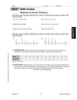


© Copyright 2026