1. business and industrial

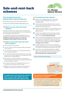
Long-Term Financial Planning and Growth
What is Financial Planning
Firms must plan for both the short term and the long term. Short-term planning rarely looks
further ahead than the next 12 months. It seeks to ensure that the firm has enough cash to pay
its bills and that short-term borrowing and lending is arranged to the best advantage. We
discuss short-term planning in the next chapter.
Here we are concerned with long-term planning, where a typical planning horizon is 5 years,
although some firms look out 10 years or more. For example, it can take at least 10 years for
an electric utility to design, obtain approval for, build, and test a major generating plant.
Long-term financial planning focuses on the firm’s long-term goals, the investment that will be
needed to meet those goals, and the finance that must be raised. However, you cannot think
about these things without also tackling other important issues. For example, you need to
consider possible dividend policies, for the more that is paid out to shareholders, the more the
external financing that will be needed. You also need to think about what is an appropriate debt
ratio for the firm. A conservative capital structure may mean greater reliance on new share
issues. The financial plan is used to enforce consistency in the way that these questions are
answered and to highlight the choices that the firm needs to make. Finally, by establishing a set
of consistent goals, the plan enables subsequent evaluation of the firm’s performance in meeting
those goals.
Financial Planning Focuses on the Big Picture
Many of the firm’s capital expenditures are proposed by plant managers. However, the final
budget must also reflect strategic plans made by senior management. Positive-NPV
opportunities occur in those businesses where the firm has a real competitive advantage.
Strategic plans need to identify such businesses and look to expand them. The plans also seek
to identify businesses to sell or liquidate as well as businesses that should be allowed to run
down.
Strategic planning involves capital budgeting on a grand scale. In this process, financial planners
try to look at the investment by each line of business and avoid getting bogged down in details.
Of course, some individual projects are large enough to have significant individual impact. For
example, the telecom giant Verizon recently announced its intention to spend billions of dollars
to deploy fiber-optic-based broadband technology to its residential customers, and you can bet
that this project was explicitly analyzed as part of its long-range financial plan. Normally,
however, financial planners do not work on a project-by-project basis. Smaller projects are
aggregated into a unit that is treated as a single project.
Long-Term Planning Handout R1.Docx
Page 1
At the beginning of the planning process, the corporate staff might ask each division to submit
three alternative business plans covering the next 5 years:
1: A best-case or aggressive growth plan calling for heavy capital investment and rapid
growth of existing markets.
2: A normal growth plan in which the division grows with its markets but not
significantly at the expense of its competitors.
3: A plan of retrenchment if the firm’s markets contract. This is planning for lean
economic times.
The plan will contain a summary of capital expenditures, working capital requirements, as well
as strategies to raise funds for these investments.
Growth as a Financial Management Goal
Why Build Financial Plans?
Firms spend considerable energy, time, and resources building elaborate financial plans. What
do they get for this investment?
Examining Interactions
Contingency Planning
Planning is not just forecasting. Forecasting concentrates on the most likely outcomes, but
planners need to worry about unlikely events as well as likely ones. If you think ahead about
what could go wrong, then you are less likely to ignore the danger signals and you can respond
faster to trouble.
Companies have developed a number of ways of asking ―what-if‖ questions about both
individual projects and the overall firm. For example, managers often work through the
consequences of their decisions under different scenarios. One scenario might envisage high
interest rates contributing to a slowdown in world economic growth and lower commodity
prices. A second scenario might involve a buoyant domestic economy, high inflation, and a weak
currency.
The idea is to formulate responses to inevitable surprises. What will you do, for example, if
sales in the first year turn out to be 10 percent below forecast? A good financial plan should
help you adapt as events unfold.
Considering Options
Planners need to think whether there are opportunities for the company to exploit its existing
strengths by moving into a wholly new area. Often they may recommend entering a market for
―strategic‖ reasons—that is, not because the immediate investment has a positive net present
value but because it establishes the firm in a new market and creates options for possibly
valuable follow-on investments.
Page 2
Long-Term Planning Handout R1.Docx
For example, Verizon’s costly fiber-optic initiative would never be profitable strictly in terms of
its current uses, for phone or conventional Internet applications. However, the new technology
gives Verizon options to offer services that may be highly valuable in the future, such as the
rapid delivery of an array of home entertainment services. The justification for the huge
investment lies in these potential growth options.
Forcing Consistency & Ensuring Feasibility
Financial plans describe the connections between the firm’s plans for growth and the financing
requirements. For example, a forecast of 25 percent growth might require the firm to issue
securities to pay for necessary capital expenditures, while a 5 percent growth rate might enable
the firm to finance capital expenditures by using only reinvested profits.
Financial plans should help to ensure that the firm’s goals are mutually consistent. For example,
the chief executive might say that she is shooting for a profit margin of 10 percent and sales
growth of 20 percent, but financial planners need to think whether the higher sales growth may
require price cuts that will reduce profit margin.
Moreover, a goal that is stated in terms of accounting ratios is not operational unless it is
translated back into what that means for business decisions. For example, a higher profit margin
can result from higher prices, lower costs, or a move into new, high-margin products. Why
then do managers define objectives in this way? In part, such goals may be a code to
communicate real concerns. For example, a target profit margin may be a way of saying that in
pursuing sales growth, the firm has allowed costs to get out of control.
The danger is that everyone may forget the code and the accounting targets may be seen as
goals in themselves. No one should be surprised when lower-level managers focus on the goals
for which they are rewarded. For example, when Volkswagen set a goal of 6.5 percent profit
margin, some VW groups responded by developing and promoting expensive, high-margin cars.
Less attention was paid to marketing cheaper models, which had lower profit margins but
higher sales volume. In 2002 Volkswagen announced that it would de-emphasize its profit
margin goal and would instead focus on return on investment. It hoped that this would
encourage managers to get the most profit out of every dollar of invested capital.
Avoiding Surprises
Financial Planning has three important uses:
Long-Term Planning Handout R1.Docx
Page 3
The following steps are used to develop a financial forecast:
Financial Planning Models
Financial planners often use a financial planning model to help them explore the consequences
of alternative financial strategies. These models range from simple models, such as the one
presented later in this chapter, to models that incorporate hundreds of equations.
Financial planning models support the financial planning process by making it easier and cheaper
to construct forecast financial statements. The models automate an important part of planning
that would otherwise be boring, time-consuming, and labor-intensive.
Programming these financial planning models used to consume large amounts of computer time
and high-priced talent. Microsoft Excel is regularly used to solve complex financial planning
problems.
Components of a Financial Planning Model
A completed financial plan for a large company is a substantial document. A smaller
corporation’s plan would have the same elements but less detail. For the smallest businesses,
financial plans may be entirely in the financial managers’ heads. The basic elements of the plans
will be similar, however, for firms of any size.
A completed financial plan for a large company is a substantial document. A smaller
corporation’s plan would have the same elements but less detail. For the smallest businesses,
financial plans may be entirely in the financial managers’ heads. The basic elements of the plans
will be similar, however, for firms of any size.
Financial plans include three components: inputs, the planning model, and outputs. Let us look
at them in turn.
Inputs
The inputs to the financial plan consist of the firm’s current financial statements and its
forecasts about the future. Usually, the principal forecast is the likely growth in sales, since
many of the other variables such as labor requirements and inventory levels are tied to sales.
These forecasts are only in part the responsibility of the financial manager. Obviously, the
marketing department will play a key role in forecasting sales. In addition, because sales will
Page 4
Long-Term Planning Handout R1.Docx
depend on the state of the overall economy, large firms will seek forecasting help from firms
that specialize in preparing macroeconomic and industry forecasts.
The Planning Model
The financial planning model calculates the implications of the manager’s forecasts for profits,
new investment, and financing. The model consists of equations relating output variables to
forecasts. For example, the equations can show how a change in sales is likely to affect costs,
working capital, fixed assets, and financing requirements. The financial model could specify that
the total cost of goods produced may increase by 80 cents for every $1 increase in total sales,
that accounts receivable will be a fixed proportion of sales, and that the firm will need to
increase fixed assets by 8 percent for every 10 percent increase in sales.
Outputs
The output of the financial model consists of financial statements such as income statements,
balance sheets, and statements describing sources and uses of cash. These statements are called
pro formas, which means that they are forecasts based on the inputs and the assumptions built
into the plan. Usually the output of financial models also includes many of the financial ratios we
discussed in the last chapter. These ratios indicate whether the firm will be financially fit and
healthy at the end of the planning period.
The Plug Method
Gourmet Coffee Inc.
Balance Sheet
December 31, 2009
Assets
1,000
Total
1,000
Income Statement
For Year Ended December 31, 2009
Debt
400
Revenues
2,000
Equity
600
Costs
1,600
Total
1,000
Net Income
400
Initial Assumptions
Revenues will grow at 15%
All items are tied directly to sales, and the current relationships are optimal
Consequently, all other items will also grow at 15%
Pro Forma Income Statement Year Ended 2010
Revenues
2,300
Costs
1,840
Net Income
460
Long-Term Planning Handout R1.Docx
Page 5
Pro Forma Balance Sheet
Year Ended 2010
Case I
Assets
Debt
Dividends are the plug variable, so equity increases at 15%
Dividends = 460 – 90 = 370 dividends paid
Case II
Total
Assets
Debt is the plug variable and no dividends are paid
Debt = 1,150 – 1060 = 90
Repay 400 – 90 = 310 in debt
Page 6
Equity
Total
Debt
Equity
Total
Total
Long-Term Planning Handout R1.Docx
We will learn about other forecasting techniques using the following example.
Maggie Taylor is the financial manager of Synapse Enzymes (SE), a New Jersey producer of specialized
enzymes for use in cellulosic ethanol production, and must prepare a financial forecast for 2010. SE's
2009 sales were $2 billion, and the marketing department is forecasting a 25 percent increase for 2010.
Eduard Buchner, SE’s CEO has directed Maggie to prepare a forecast assuming the company is at full
capacity and another assuming current production is less than full capacity. The 2009 financial
statements, plus some other data, are shown below.
Table SE-1 2009 Income Statement (in millions)
Sales
$2,000.00
Variable Costs
1,200.00
Fixed Costs
EBIT
700
$100.00
Interest
20
EBT
$80.00
Taxes (40%)
$32.00
Net Income
$48.00
Dividends (40%)
$19.20
Additions to Retained Earnings
$28.80
Table SE-2 2009 Balance Sheet (in millions)
Cash and Securities
$20.00
Accounts Receivable
$240.00
Inventories
$240.00
Total Current Assets
$500.00
Net Fixed Assets
$500.00
Total Assets
$1,000.00
Accounts Payable and Accruals
$100.00
Notes Payable
$100.00
Total Current Liabilities
$200.00
Long Term Debt
$100.00
Common Stock
$500.00
Retained Earnings
$200.00
Total Liabilities and Equity
$1,000.00
Long-Term Planning Handout R1.Docx
Page 7
Table SE-3 Key Ratios (SE & Industry)
2009
Ratio
SE
Industry Formulas
Profit margin
2.40%
4.00%
ROE
6.86%
15.60%
DSO
43.80
32.00
Inventory turnover
8.33
11.00
Fixed asset turnover
4.00
5.00
Debt/Assets
30.00%
36.00%
TIE
5.00
9.40
Current ratio
2.50
3.00
NOPAT
$60.00
EBIT(1-T)
NOWC
$400.00
CA – (A/P & Accruals)
Total Net Operating Capital
$900.00
NOWC + NFA
NOPAT/Sales
3.00%
5.00%
Net Operating Capital / Sales
45.00%
35.00%
Return on Invested Capital (NOPAT/Capital) 6.67%
14.00%
You were recently hired as a Financial Analyst reporting to Ms. Taylor. Your responsibilities
include assisting in the development of the forecast. She asked you to begin by answering the
following set of questions.
Table SE-4 Forecast Inputs
Inputs
Percent growth in sales
Interest rate on debt (LT & ST)
Tax rate
Dividend Payout Ratio
25%
10%
40%
40%
Funds will be generated through:
Notes Payable:
50%
Long-Term Debt:
50%
Page 8
Long-Term Planning Handout R1.Docx
1) Assume that SE was operating at full capacity in 2009 with respect to all assets, therefore
all assets must grow proportionally with sales, accounts payable and accruals will also
grow in proportion to sales, and the 2009 profit margin and dividend payout will be
maintained. Under these conditions, what will the company's financial requirements be
for the coming year? Use the EFN equation to answer this question.
The EFN Equation is:
If EFN is positive, then you must secure additional financing.
If EFN is negative, then you have more financing than is needed.
Pay off debt.
Buy back stock.
Buy short-term investments.
2) How would changes in these items affect the EFN? (Consider each item separately and
hold all other things constant.)
Sales increase
Increases asset requirements, increases EFN
Dividend payout ratio increases
Reduces funds available internally, increases EFN
Profit margin increases
Increases funds available internally, decreases EFN
Capital intensity ratio increases
Increases asset requirements, increases EFN
SE begins paying its suppliers sooner.
Decreases spontaneous liabilities, increases EFN
Long-Term Planning Handout R1.Docx
Page 9
3) Now estimate the 2010 financial requirements using the percent of sales method.
Project sales based on forecasted growth rate in sales
Forecast some items as a percent of the forecasted sales
Table SE-5 2010 Forecast
2009 Income Statement
Percent of Sales
2010 Forecast
(in millions)
Sales
Variable Costs
Fixed Costs
EBIT
$2,000.00
$2,500.00
1,200.00
0.6000
1,500.00
700.00
0.3500
875.00
$100.00
$125.00
20.00
20.00
EBT
$80.00
$105.00
Taxes (40%)
$32.00
$42.00
Net Income
$48.00
$63.00
Dividends (40%)
$19.20
$25.20
Additions to Retained Earnings
$28.80
$37.80
Interest
Page 10
Long-Term Planning Handout R1.Docx
Table SE-5 2010 Forecast (Continued)
Percent
2009 Balance Sheet (in millions)
of Sales
Cash and Securities
$20.00
0.0100
Accounts Receivable
$240.00
0.1200
Inventories
$240.00
0.1200
Total Current Assets
$500.00
Net Fixed Assets
$500.00
Total Assets
$625.00
0.2500
$1,000.00
$1,250.00
Accounts Payable and Accruals
$100.00
Notes Payable
$100.00
$100.00
Total Current Liabilities
$200.00
$225.00
Long Term Debt
$100.00
$100.00
Common Stock
$500.00
$500.00
Retained Earnings
$200.00
$237.80
$1,000.00
$1,062.80
Total Liabilities and Equity
0.0500
Required assets =
$1,250.00
Specified sources of financing =
$1,062.80
External funds needed (EFN) =
$187.20
SE has a choice when considering other items
Long-Term Planning Handout R1.Docx
Page 11
We assumed:
Each type of asset, as well as payables, accruals, and fixed and variable costs, will be the same
percent of sales in 2010 as in 2009
The payout ratio is held constant at 40 percent
External funds needed are financed 50 percent by notes payable and 50 percent by long-term
debt (no new common stock will be issued)
All debt carries an interest rate of 10 percent
Interest expenses should be based on the average of the beginning and ending debt values.
Interest expense is actually based on the daily balance of debt during the
year.
There are three ways to approximate interest expense. Base it on:
Debt at end of year
Debt at beginning of year
Average of beginning and ending debt
Basing Interest Expense on Debt at End of Year
Will over-estimate interest expense if debt is added throughout the year
instead of all on January 1.
Causes circularity called financial feedback: more debt causes more interest,
which reduces net income, which reduces retained earnings, which
causes more debt, etc.
Basing Interest Expense on Debt at the Beginning of Year
Will under-estimate interest expense if debt is added throughout the year
instead of all on December 31.
But doesn’t cause problem of circularity
Basing Interest Expense on Average of Beginning and Ending Debt
Will accurately estimate the interest payments if debt is added smoothly
throughout the year.
But has problem of circularity.
Page 12
Long-Term Planning Handout R1.Docx
Table SE-6 2010 Forecast
Percent
2009 Income Statement
of Sales
(in millions)
From
Table SE-5
Without EFN
Sales
$2,000.00
Variable Costs
2010
2010
Forecast
Feedback
1st Pass
Forecast
Feedback
2nd Pass
$2,500.00
$2,500.00
$2,500.00
1,200.00
0.6000
1,500.00
1,500.00
1,500.00
700.00
0.3500
875.00
875.00
875.00
$100.00
$125.00
$125.00
$125.00
20.00
20.00
29.53
EBT
$80.00
$105.00
$95.47
Taxes (40%)
$32.00
$42.00
$38.19
Net Income
$48.00
$63.00
Dividends (40%)
$19.20
$25.20
Additions to Retained Earnings
$28.80
$37.80
Fixed Costs
EBIT
Interest
2009 Balance Sheet
(in millions)
Cash and Securities
$20.00
0.0100
$25.00
$25.00
$25.00
Accounts Receivable
$240.00
0.1200
$300.00
$300.00
$300.00
Inventories
$240.00
0.1200
$300.00
$300.00
$300.00
$625.00
$625.00
$625.00
$625.00
$625.00
$625.00
$1,250.00
$1,250.00
$1,250.00
$125.00
$125.00
$125.00
Total Current Assets
Net Fixed Assets
$500.00
$500.00
0.2500
Total Assets
$1,000.00
Accounts Payable and Accruals
$100.00
Notes Payable
$100.00
$100.00
$200.00
$225.00
Long Term Debt
$100.00
$100.00
Common Stock
$500.00
$500.00
$500.00
$500.00
Retained Earnings
$200.00
$237.80
$234.43
$234.37
$1,000.00
$1,062.80
$1,246.63
$1,249.94
Required assets =
$1,250.00
$1,250.00
$1,250.00
Specified sources of financing =
$1,062.80
$1,246.63
$1,249.94
External funds needed (EFN) =
$187.20
$3.37
$0.06
Total Current Liabilities
Total Liabilities and Equity
Long-Term Planning Handout R1.Docx
0.0500
$93.60
$193.60
$1.68
$318.60
$93.60
$193.60
$195.28
$320.28
$1.68
$195.28
Page 13
4) Why does the percent of sales approach produce a somewhat different EFN than the
equation approach? Which method provides the more accurate forecast?
Equation method assumes a constant profit margin.
Pro forma method is more flexible. More important, it allows
different items to grow at different rates.
5) Calculate SE's forecasted ratios, and compare them with the company's 2009 ratios and
with the industry averages. Calculate SE’s forecasted free cash flow and return on
invested capital (ROIC).
Table SE-7 2010 Forecast Ratios
2009
2010
Ratio
Formulas
Key Ratios
SE
Industry
2nd Pass
Profit margin
2.40%
4.00%
2.29%
ROE
6.86%
15.60%
7.80%
DSO
43.80
32.00
43.80
Inventory turnover
8.33
11.00
8.33
Fixed asset turnover
4.00
5.00
4.00
Debt/Assets
30.00%
36.00%
41.25%
TIE
5.00
9.40
4.23
Current ratio
2.50
3.00
1.95
NOPAT
$60.00
$75.00
EBIT(1-T)
NOWC
$400.00
$500.00
CA – (A/P & Accruals)
Total Net Operating Capital
$900.00
$1,125.00 NOWC + NFA
NOPAT/Sales
3.00%
5.00%
3.00%
Net Operating Capital / Sales 45.00%
35.00%
45.00%
ROIC (NOPAT/Capital)
14.00%
6.67%
Investment in Capital
Page 14
6.67%
$225.00
Long-Term Planning Handout R1.Docx
Table SE-8 2010 Forecast Free Cash Flows and Other Information
Forecast
Free Cash Flow Calculation
NOPAT
2009
2010
100(1 – 0.40) =
= 125(1 – 0.40)
Net operating working capital
(NOWC)
500 – 100 =
= 625 - 125
Total Operating Capital
400 + 500 =
= 500 + 625
Investment in Capital
= 1,125 - 900
FCF
= 75 - 225
Return on Invested Capital
(NOPAT/Capital)
Industry
14.00%
Remember Cash Flow from Assets for Fin 311
CFA = OCF – Net Capital spending – ∆NWC
Operating cash flow (OCF) = EBIT + Dep – Taxes = EBIT(1 – T) + Dep
Net Capital Spending = NFAEnd – NFABeg + Dep
∆NOWC = NOWCEnd - NOWCBeg
6) Based on comparisons between SE's days sales outstanding (DSO) and inventory turnover
ratios with the industry average figures, does it appear that SE is operating efficiently with
respect to its inventory and accounts receivable? Suppose SE were able to bring these
ratios into line with the industry averages. What effect would this have on its EFN and its
financial ratios? What effect would this have on free cash flow and ROIC?
Long-Term Planning Handout R1.Docx
Page 15
Table SE-9 2010 Forecast with Ratio Improvements
Ratio Improvements
DSO
32.00
Inventory turnover
11.00
2009 Income Statement
Percent
2010
of Sales
Forecast
(in millions)
Without EFN
Feedback
1st Pass
Feedback
2nd Pass
Sales
$2,000.00
$2,500.00
$2,500.00
$2,500.00
Variable Costs
1,200.00
0.6000
1,500.00
1,500.00
1,500.00
Fixed Costs
700.00
0.3500
875.00
875.00
875.00
EBIT
$100.00
$125.00
$125.00
$125.00
Interest
20.00
EBT
$80.00
$105.00
$103.29
Taxes (40%)
$32.00
$42.00
$41.31
Net Income
$48.00
$63.00
$61.97
Dividends (40%)
$19.20
$25.20
$24.79
Additions to Retained Earnings
$28.80
$37.80
$37.18
20.00
2009 Balance Sheet
Percent
(in millions)
of Sales
Cash and Securities
$20.00
Accounts Receivable
25.00
$21.71
21.71
$25.00
$25.00
$240.00
$219.18
$219.18
Inventories
$240.00
$227.27
$227.27
Total Current Assets
$500.00
$471.45
$471.45
Net Fixed Assets
$500.00
$625.00
$625.00
Total Assets
$1,000.00
$1,096.45
$1,096.45
Accounts Payable and Accruals
$100.00
$125.00
$125.00
Notes Payable
$100.00
$100.00
Total Current Liabilities
$200.00
$225.00
Long Term Debt
$100.00
$100.00
Common Stock
$500.00
$500.00
$500.00
Retained Earnings
$200.00
$237.80
$237.18
Total Liabilities and Equity
$1,000.00
$1,062.80
$1,096.44
Required assets =
$1,096.45
$1,096.45
Specified sources of financing =
$1,062.80
$1,096.44
External funds needed (EFN) =
$33.65
$0.01
Page 16
0.0100
$21.68
0.2500
0.0500
$125.00
$16.83
$0.30
$117.13
$242.13
$16.83
$0.30
$117.13
Long-Term Planning Handout R1.Docx
Table SE-10 2010 Key Ratio Forecast
2009
2010
Ratio
Key Ratios
SE
Industry
2nd Pass Formulas
Profit margin
2.40%
4.00%
2.48%
ROE
6.86%
15.60%
8.41%
DSO
43.80
32.00
32.00
Inventory turnover
8.33
11.00
11.00
Fixed asset turnover
4.00
5.00
4.00
Debt/Assets
30.00%
36.00%
32.77%
TIE
5.00
9.40
5.76
Current ratio
2.50
3.00
1.95
NOPAT
$60.00
$75.00
EBIT(1-T)
NOWC
$400.00
$346.45
CA – (A/P & Accruals)
Total Net Operating Capital
$900.00
$971.45
NOWC + NFA
NOPAT/Sales
3.00%
5.00%
3.00%
Net Operating Capital / Sales 45.00%
35.00%
38.86%
ROIC (NOPAT/Capital)
14.00%
7.72%
6.67%
Investment in Capital
Long-Term Planning Handout R1.Docx
$71.45
Page 17
Table SE-11 2010 Free Cash Flow and Other Forecasts
Forecast
Free Cash Flow
NOPAT
2009
100(1 – 0.40) =
2010
= 125(1 – 0.40)
Net operating working capital
(NOWC)
500 – 100 =
= 471.45 - 125
Total Operating Capital
400 + 500 =
= 346.45 + 625
Investment in Capital
= 971.45 - 900
FCF
= 75 – 71.45
Return on Invested Capital
(NOPAT/Capital)
Industry
14.00%
7) In addition to improving the ratios considered above what if SE was able to control Selling
and Admin Cost? Specifically, what if fixed costs were decreased to 33 percent of sales?
What effect would this have on its EFN and its financial ratios? What effect would this
have on free cash flow and ROIC?
Page 18
Long-Term Planning Handout R1.Docx
Table SE-12 2010 Forecast with Ratio Improvements & Cost Reduction
Ratio & Cost Improvements
DSO:
32.00
Inventory turnover:
11.00
Fixed Costs:
33%
Percent
2009 Income Statement
of Sales
(in millions)
2010 Forecast
Without EFN
Feedback
With EFN
Feedback
With EFN
Sales
$2,000.00
$2,500.00
$2,500.00
$2,500.00
Variable Costs
1,200.00
0.6000
1,500.00
1,500.00
1,500.00
Fixed Costs
700.00
0.3300
825.00
825.00
EBIT
$100.00
$175.00
$175.00
Interest
20.00
EBT
$80.00
$154.20
Taxes (40%)
$32.00
$61.68
Net Income
$48.00
$92.52
Dividends (40%)
$19.20
$37.01
Additions to Retained Earnings
$28.80
$55.51
$20.78
$20.80
20.80
Percent
2009 Balance Sheet (in millions)
of Sales
Cash and Securities
$20.00
Accounts Receivable
0.0100
$25.00
$25.00
$25.00
$240.00
$219.18
$219.18
$219.18
Inventories
$240.00
$227.27
$227.27
$227.27
Total Current Assets
$500.00
$471.45
$471.45
$471.45
Net Fixed Assets
$500.00
$625.00
$625.00
$625.00
Total Assets
$1,000.00
$1,096.45
$1,096.45
$1,096.45
Accounts Payable and Accruals
$100.00
$125.00
$125.00
$125.00
Notes Payable
$100.00
$100.00
Total Current Liabilities
$200.00
$225.00
Long Term Debt
$100.00
$100.00
Common Stock
$500.00
$500.00
Retained Earnings
$200.00
Total Liabilities and Equity
$1,000.00
0.2500
0.0500
$7.83
$107.83
$0.14
$232.83
$7.83
$107.83
$500.00
$107.97
$232.97
$0.14
$107.97
$500.00
$255.51
$1,080.80
$1,096.17
$1,096.45
Required assets =
$1,096.45
Specified sources of financing =
$1,096.45
External funds needed (EFN) =
$0.01
Long-Term Planning Handout R1.Docx
Page 19
Table SE-13 2010 Key Ratio Forecast
2009
2010
Ratio
Formulas
Key Ratios
SE
Industry
2nd Pass
Profit margin
2.40%
4.00%
3.70%
ROE
6.86%
15.60%
12.25%
DSO
43.80
32.00
32.00
Inventory turnover
8.33
11.00
11.00
Fixed asset turnover
4.00
5.00
4.00
Debt/Assets
30.00%
36.00%
31.09%
TIE
5.00
9.40
8.41
Current ratio
2.50
3.00
2.02
NOPAT
$60.00
$105.00
EBIT(1-T)
NOWC
$400.00
$346.45
CA – (A/P & Accruals)
Total Net Operating Capital
$900.00
$971.45
NOWC + NFA
NOPAT/Sales
3.00%
5.00%
4.20%
Net Operating Capital / Sales 45.00%
35.00%
38.86%
ROIC (NOPAT/Capital)
14.00%
10.81%
Investment in Capital
Page 20
6.67%
$71.45
Long-Term Planning Handout R1.Docx
Table SE-14 2010 Free Cash Flow and Other Forecasts
Forecast
Free Cash Flow
2009
2010
$60.00
$105.00
= 175(1 – 0.40)
Net operating working capital
(NOWC)
500 – 100 = $400.00
$346.45
= 471.45 - 125
Total Operating Capital
400 + 500 = $900.00
$971.45
= 346.45 + 625
Investment in Capital
$71.45
= 971.45 - 900
FCF
$33.55
= 105 – 71.45
NOPAT
Return on Invested Capital
(NOPAT/Capital)
Long-Term Planning Handout R1.Docx
100(1 – 0.40) =
10.81%
Industry
14.00%
Page 21
8) Suppose you now learn that SE's 2009 receivables and inventories were in line with
required levels, given the firm's credit and inventory policies, but that excess capacity
existed with regard to fixed assets. Specifically, fixed assets were operated at only 75
percent of capacity.
What level of sales could have existed in 2009 with the available fixed assets?
Effect of Excess Capacity
Suppose in 2009 fixed assets had been operated at only 75% of capacity?
Capacity Sales = Actual Sales/% of Capacity
How would the existence of excess capacity in fixed assets affect the additional funds needed
during 2010?
Forecasted sales are less than this, so no new fixed assets are needed.
Table SE-15
Previously forecasted EFN = $187.20 From Table SE-6
Previously forecasted addition to fixed assets = $125.00 From Table SE-6
EFN if there is excess capacity =
$62.20
If Sales went up to $3,000, not $2500, what would the F.A. requirement be?
Target Ratio = Fixed Assets/ Capacity Sales
Target Ratio =
Target Ratio =
Change in FA =
Change in FA =
Change in CA =
Change in CL =
Change in R/E =
EFN =
Page 22
Long-Term Planning Handout R1.Docx
9) The relationship between sales and the various types of assets is important in financial
forecasting. The percent of sales approach, under the assumption that each asset item
grows at the same rate as sales, leads to an EFN forecast that is reasonably close to the
forecast using the EFN equation. Explain how each of the following factors would affect
the accuracy of financial forecasts based on the EFN equation:
Economies of scale in the use of assets
Economies of scale: leads to less-than-proportional asset increases.
Lumpy assets.
Lumpy assets: leads to large periodic EFN requirements, recurring excess capacity.
External Financing and Growth
Table SE-15 shows that at low sales growth rates, SE will have a surplus of cash. When the
growth rate is 6.88 percent, Se requires external funds.
Table SE-15
Sales Growth Increase FA Add R/E
0%
0
28.8
5%
50
30.6
10%
100
32.4
15%
150
34.2
20%
200
36.0
25%
250
37.8
30%
300
39.6
35%
350
41.4
Graph SE-1
400.00
350.00
300.00
250.00
200.00
150.00
100.00
50.00
0.00
0%
5%
10%
15%
Add R/E
Long-Term Planning Handout R1.Docx
20%
25%
30%
35%
Increase FA
Page 23
Internal and Sustainable Growth Rates
The internal growth rate is the maximum growth a firm can be achieved with internally
generated funds. The equation is:
For SE:
Determinants of Growth
Profit Margin
Dividend Policy
Financial Policy
Total Asset Turnover
Page 24
Long-Term Planning Handout R1.Docx