
The Role of Soft Information in Subprime Mortgage Lending
A Theory of Subprime Mortgage Lending
with Appliactions to The Rise and Fall of
the Subprime Conduit Mortgage Market
Jaime Luque
University of Wisconsin - Madison
Timothy Riddioughy
University of Wisconsin - Madison
May 8, 2015
Abstract
We present a general equilibrium model of a subprime economy characterized
by limited recourse mortgages, asymmetric borrower credit quality information, and
mortgage lenders that either own or sell the loans they originate. We identify several components in the equilibrium mortgage rate, including the access to soft credit
information, the foreclosure recovery rate, and the liquidity in the securitized investment market. We show that the equilibrium size of the subprime lending market can
expand and contract depending on the access to liquidity in the securitized investment market and the predictive power of the credit scoring technology. Our theory
rationalizes the emergence of the subprime conduit mortgage market and subsequent
collapse of the traditional lending model, and also the recent rise and fall of the
subprime conduit mortgage market. In addition, the model sheds some light on the
access to and fragmentation of the rental and owner-occupied segments of the housing
market. A number of extensions to the model are considered to assess its robustness.
Key words: subprime lending; soft information; credit scoring technology; portfolio lenders; conduit lenders; originate-to-distribute lending model; equilibrium;
mortgage market collapses.
JEL Classi…cation numbers: R21, R3, R52, D4, D5, D53.
y
[email protected]
[email protected]
1
1
Introduction
1.1
Motivation
The mortgage lending market has experienced a dramatic change during the last couple
of decades. New non-traditional lenders, such as brokers, ventured capitalists and hedge
funds, turned to the subprime market seeking higher returns in a low-rate environment.
Their main lending model was to originate mortgages and distribute them to secondary
market security investors. Such lenders faced far less regulatory scrutiny than traditional
banks did, and heavily relied on the available mortgage credit scoring technology to evaluate
a consumer’s credit risk pro…le. Subprime mortgages were negotiated by phone based on
observable hard credit information, such as credit history and FICO scores. Soft information acquisition was at best limited.1 The result was an unprecedented boom in subprime
mortgage lending that started in the early 2000s and ended up with the collapse of Lehman
Brothers in 2008. This paper attempts to rationalize the emergence of the subprime conduit mortgage market and its dominance over the traditional relationship lending model,
and also the recent rise and fall of subprime mortgage lending.
1.2
Description of the model
Our theory of the subprime mortgage market relies on a general equilibrium model of
a subprime economy characterized by limited recourse mortgages, asymmetric borrower
credit quality information, and mortgage lenders that either own or sell the loans they
originate. We naturally incorporate asymmetric information in the subprime mortgage
market by allowing for unobserved borrower heterogeneity in credit risk and di¤erentiating
between two types of lenders: portfolio and conduit lenders.
Portfolio lenders originate-to-own, and as such are subject to lending capacity constraints. They can further be thought of as traditional relationship lenders with a comparative advantage in their ability to acquire soft credit risk information at low cost. Loan
pricing therefore is risk-based, but the determinants of the loan price are not fully observable to outsiders that only have access to hard credit information. In contrast, conduit
lenders primarily (but not necessarily exclusively) originate-to-distribute, and hence are
transactions-based. These agents generally assess credit risk based on hard information
only, but in doing so recognize that their borrower-lending clientele is lower credit quality
on average. Thus, due to this di¤erent capability to resolve credit information asymmetries
at low cost, portfolio lenders incorporate soft information into the determination of a (borrower speci…c) risk-based subprime loan rate, while conduit lenders instead pool borrowers
and choose the rate based on the use of hard information only.
The conduit mortgage yield contains a negative adverse selection component, captued
by the lack of soft information, but also a positive liquidity component coming from the
1
Soft information may include listening to and analyzing the borrower’s explanation for past di¢ culties
in making credit payments and determining whether the hard numbers for the borrower or property make
sense given what a loan agent can perceive about them. For a discussion of how securitization discourages
lenders from engaging in “soft” mortgage underwriting, see "Comments to the Federal Deposit Insurance
Corporation" by the National Association of Consumer Advocates on February 22, 2010.
2
conduit lender’s access to the securitized investment market. When the distribution rate
of mortgages to investors increases, the negative e¤ect of adverse selection on the mortgage discount price is o¤set moreby the higher valuation that investors assign to conduit
mortgages. This trade-o¤ is one of the key drivers of the rise and fall of subprime conduit
lending market in our model: securitization allows customization, which lowers the cost
of capital in the conduit loan market. When the liquidity in the securitized investment
market is high, the conduit mortgage rate can become smaller than the portfolio loan rate
even when some degree of adverse selection is present in the conduit loans market.
Our model rationalizes the emergence of the subprime conduit mortgage market and
dominance over the traditional lending model. When securitization of subprime mortgages
found a niche in the secondary securties market and new credit scoring technologies, such as
FICO scores and consumer’s credit history, become available, non-traditional lenders, such
as brokers, ventured capitalists and hedge funds, turned to the subprime market seeking
higher returns in a low-rate environment. As our theory shows, when investors’ apetite
for subprime mortgage-backed securities is high, the conduit mortgage rate may decrease
below what the traditional portfolio lenders charge for their mortgages. This happens even
when these non-traditional lenders relied on an imperfect credit scoring technology. The
result is that all higher quality borrowers prefer to migrate to the subprime conduit lending
market leaving portfolio lenders with a smaller market share.
The subprime conduit mortgage market can also collapse in our model. We identify
a regime where both portfolio lenders and conduit lenders actively lend to di¤erent pools
of borrowers at di¤erent mortgage rates. If, however, the quality of the pool of borrowers
in the conduit loan market deteriorates su¢ ciently, the subsidy paid by the higher quality
borrowers to support a pooling loan rate is so high that discourages home ownership. High
credit quality consumers that were not able to borrow from portfolio lenders would then
leave the conduit loan market, resulting in the collapse of this market. Alternatively, the
conduit market can also collapse in our model due to land use regulation that prevents
subprime borrowers with small loans from buying houses with lot size below a minimum
threshold. This result illustrates how housing regulations, in the form of costs associated
with minimum lot and house size constraints, which are often imposed by local land use
regulators, prevent the least well-endowed subprime consumers who cannot a¤ord from
purchasing a house a minimum lot size.
The rise and fall of subprime lending is best described in terms of our model as follows. The rise occurs when hard information has better predictive power, soft information
is easier to acquire, regulation on mortgage securitization is more lax, investors are less
anxious, and foreclosure costs decrease. When one or several factors occur simultaneously
the conduit loan market expands and loan originations increase. This in turn translates
into higher owner-occupied house prices and lower credit spreads for conduit loans. The
fall, on the hand, occurs when lending standards seriously deteriorate (undisciplined conduit lenders have not properly invested in acquiring soft information), investors are more
anxious, liquidity in the secondary securities market drys, and foreclosure costs increase.
In this case, the conduit loan market shrinks. The lower access to credit lowers the demand
for owner-occupied housing and decreases equilibrium house prices.
3
1.3
Relationship with the literature
The literature on collateralized lending with asymmetric information is vast and has expanded rapidly in recent years in light of the subprime mortgage lending and …nancial crisis.
In brief, and at a high level, this paper contributes to the literature that studies how both
information frictions and mortgage securitization possibilities a¤ect debt contract design,
mortgage originations, securitization, and house prices.2
Our equilibrium analysis of the subprime mortgage market also contributes to the recent empirical literature that attempts to identify the pricing determinants of di¤erences
between portfolio loans and conduit loans, and also di¤erences among di¤erent types of
conduit loans themselves (see Keys, Mukherjee, Seru, and Vig (2010) and Krainer and
Laderman (2014))3 . Agarwal, Amromin, Ben-David, Chomsisengphet and Evano (2011)
recognized the lack of a theoretical model. To this extent, our paper provides the …rst theoretical framework that enables to decompose the conduit mortgage spread into a credit
information component, a foreclosure recovery rate component, and a component that captures the access to liquidity in the securitized investment market. We then show how these
di¤erent pricing components can drive the rise and fall of the subprime conduit mortgage
market.
Our pricing results also have some analogies with Sato’s (2015) analysis of transparent versus opaque assets. Sato shows that transparent …rms own transparent assets and
opaque …rms own opaque assets in equilibrium. This is analogous to us showing portfolio
lenders hold only higher quality loans and conduit lenders own a mix. The reasons for
such holdings are di¤erent in the two models, however. In our model, conduit lenders are
intermediaries that transform a mix of assets into very opaque subprime mortgage-backed
securities (MBS). Sato also shows that opaque assets trade at a premium to transparent
assets. This is primarily due to agency distortions in the opaque …rm. For us a premium
in opaque asset prices comes through the investors’demand for subprime MBS.4
Our paper is also related to the literature of shadow banking and subprime lending. As
in Gennaioli, Shleifer, and Vishny (2012), our model shows that investors’wealth drives up
securitization, but in addition our model is able to generate the result that adverse selection
in the loan origination market can be the only reason why the conduit loan market shuts
down, even when there is investors’ appetite for mortgage-backed securities. Our paper
also departs from Mayer, Piskorski, and Tchistyi (2013), Makarov and Plantin (2013),
2
See Ja¤ee and Russell (1976), Stiglitz and Weiss (1981) and Akerlof (1986) for classic papers on the
e¤ects of information frictions on screening, sorting and borrower default. For recent work that focuses
on how di¤erent lenders’information sets a¤ect mortgage loan outcomes, borrowers’default, and market
unraveling, see, e.g., Karlan and Zinman (2009), Adams et al. (2009), Edelberg (2004), Rajan, Seru
and Vig (2010), and Einav et al. (2013). See Miller (2014) for a related analysis of the importance of
information provision to subprime lender screening. More generally, see Stein (2002) for a description of
how private information includes soft information, and how di¢ cult is to communicate soft information
to other agents at a distance. See also Inderst (2008) for a model that suggests a strong complementarity
between competition and the adoption of hard-information lending techniques.
3
See also Adelino, Gerardi and Willen (2013), Agarwal, Chang, and Yavas (2012), Agarwal, Amromin,
Ben-David, Chomsisengphet and Evano (2011), Ambrose, Lacour-Little, and Sanders (2005), Bubb and
Kaufman (2014), and Piskorski, Seru and Vig (2010)).
4
For a similar result in the commercial mortgage market, see An, Deng and Gabriel (2011) who …nd
that conduit loans enjoyed a 34 basis points pricing advantage over portfolio loans in the CMBS market.
4
and Piskorski and Tchistyi (2011) by distinguishing between shadow bank and formal bank
funding models, and relating their change in market share to di¤erent equilibrium subprime
mortgage con…guration regimes that result from changes in the credit scoring technology,
securitization, foreclosure costs, or lenders’capacity constraints.5
Importantly, our model captures the ebbs and ‡ows of shadow bank activity, often
peaking just prior to a downturn. The peak corresponds with poor access to soft information
acquisition by conduit lenders and high liquidity ‡owing from security investors to conduit
lenders (which is their largest if not exclusive source of funds).6 This is consistent with
Purnanandam’s (2010) evidence that lack of screening incentives coupled with leverageinduced risk-taking behavior signi…cantly contributed to the current subprime mortgage
crisis. Our equilibrium mechanism links subprime mortgage lending standards to the runup and eventually collapse in home-prices (endogenously determined in our model), and
thus …lls a gap in the literature that studies mortgage leverage and the foreclosure crisis
(Corbae and Quintin (2015)).7 Our model also di¤ers from Ordonez’s (2014) theory that
crisis appear when mortgage-backed security investors neglect systemic risks by focusing
instead on the information problems that are speci…c to the conduit loan origination market.
Our thoery has its foundations on the general collateral equilibrium model introduced
by Geanakoplos (1997, 2003) and Geanakoplos and Zame (2014). There are several di¤ences for their model and ours though. First, we consider limited recourse mortgages, which
are speci…c to the subprime mortgage market. Under this contract a good type borrower
can credibly commit to pay back the loan even even if the loan repayment is higher than
the house value.8 However, the nature of the contract protects the subprime borrower from
consuming less than a subsistence rent. Because bad type borrowers misrepresent their
type, they are not able to simultaneously honor they loan payment (designed for a good
type borrower) and consume the subsistence rent. Therefore, in our model, the lemons
in the conduit mortgage market end up defaulting and giving all their wealth, including
their housing asset, to the lenders. Hence, the limited recourse mortgage is e¤ectively a
non-recourse mortgage for the bad type borrowers (the lemons). A second aspect is that we
let households make endogenous rent versus own decisions by considering di¤erent housing
contract durations - owner-occupied (two periods contract) versus rental (one period contract) -, and thus we bring the tenure housing decision into a general equilibrium model.
A third di¤erence is that in our model home ownership requires mortgage debt …nancing
originating from two potential sources: portfolio lenders and conduit lenders. We then
5
Recent papers in the literature of shadow banking and subprime lending are Ashcraft and Schuermann
(2008), Bernake (2008), European Central Bank (2008), Keys, Mukherjee, Seru and Vig (2010), Geanakoplos (2010a, 2010b), Mishkin (2008), Purnanandam (2011), Quintin and Corbae (2015), and Keys et al
(2013); see also Calem, Covas, and Wu (2013) and Fuster and Vickery (forthcoming) for evidence of a
collapse of the private label RMBS market during the …nancial crisis.
6
As Ashcraft, Adrian, Boesky and Pozsar (2012) point out, at the eve of the …nancial crisis, the volume
of credit intermediated by the shadow banking system was close to $20 trillion, or nearly twice as large as
the volume of credit intermediated by the traditional banking system at roughly $11 trillion.
7
Other relevant papers that study foreclosure dynamics while taking exogenous house prices are Guler
(2014) and Cambell and Cocco (2014).
8
This occurs because the consumer prefers to consume more (owner-occupied) housing in the …rst period,
and hence borrows against all his disposable wealth of the second period, provided that he consumes the
minimum subsistence rent in the second period.
5
closely examine, together and separately, the e¤ects of conduit lenders’resolved (soft information acquisition) and unresolved (adverse selection) private information on borrower
sorting outcomes. The structural details underlying mortgage contract design and market
organization consequently feed back to a¤ect the rent versus own decision.
Our model also provides a micro-founded approach to soft information acquisition and
its consequences on the subprime mortgage market. Up to our knowledge, we are the …rst
ones to show that conduit lenders do not acquire (enough) soft information in equilibrium.
This result complements Keys, Mukherjee, Seru, and Vig’s (2010) empirical evidence that
existing securitization practices did adversely a¤ect the screening incentives of subprime
lenders.9
1.4
Paper structure
The rest of this paper is as follows. In Section 2 we present the baseline model with
two types of consumers, limited recourse mortgages, two types of lenders (conduit and
portfolio), one state of nature in the second period, and asymmetric information in the
conduit mortgage market. Section 3 presents the equilibrium de…nition, gives the result of
equilibrium existence, and also presents the pricing formulas that characterize the di¤erent
lenders’optimal mortgage rates and corresponding excess premium. Section 4 focuses on
the particular case of household’s tenure choice between owner-occupied housing and rental
housing. We will discuss the main ingredients of this model: house prices, mortgage market
collapses, and the size of the rental market. In Section 5 we discuss the policy implications
of the model, and also explain that the predictions of the baseline model do not change if we
consider instead an stochastic economy or if we consider instead the notion of a separating
equilibrium. Also there, we explain the consequences on the adverse selection problem
of considering instead non-recourse mortgage contracts. The Appendix is devoted to the
proofs.
2
The baseline two-periods model
Our baseline model consists of a two-periods deterministic economy with asymmetric information in the primary mortgage market and the following main ingredients. There are
households (h), portfolio lenders (r), conduit lenders (k), and security investors (i). Households are subprime households, and all have a …rst period subsistence endowment ! SR . In
the second period a fraction of these households experience a positive shock in their secSR
ond period endowment ! +
, e.g., some households …nd a better job while remaining
2 > !
households remain at their current income levels. Individual households possess private
information regarding their type in the …rst period. Mortgage contracts are recourse, but
9
Keys, Mukherjee, Seru, and Vig (2010) …nd that conditional on being securitized, the portfolio with
greater ease of securitization defaults by around 10% to 25% more than a similar risk pro…le group with a
lesser ease of securitization. Their results are con…ned to loans where intermediaries’screening e¤orts may
be relevant and soft information about borrowers determines their creditworthiness. Bubb and Kaufman
(2014), on the other hand, study the e¤ect of the moral hazard of securitization on lenders creening, and
conclude that securitization did not lead to lax screening.
6
subject to some ungarnishable minimum subsistence consumption (! SR ) by the borrower.
Thus, the only source of default is the borrower’s bad income realization. Lenders cannot
perfectly screen the type of borrowers using hard information only; only additional soft
information can identify the type of borrower. In this economy investors rely on the same
credit scoring technology than those lenders without soft information. Thus, we leave aside
the possibility of adverse selection in the secondary market of mortgage backed securities.
We also ignore any agency issues regarding securitization and its implications on distressed
loans.10
We …nd convenient to denote an agent type by a = h; r; k; i, the set of agents of type
a by A(a), and the whole set of all agents in the economy by A. The non-atomic measure
space of agents in this economy is given by (A;A; ), where A is a -algebra of subsets of
the set of agents A, and is the associated Lebesgue measure. The measure of the set of
type t = G; B consumers is set to be equal to 1, i.e., (A(l)) = 1. Also, the measures of
portfolio lenders, conduit lenders and investors are all set to be equal to 1, i.e., (A(l)) = 1
for both l = r; k and (A(i)) = 1.
2.1
Subprime households
Let us consider a two-periods economy with a continuum of consumers that we will call
subprime consumers. These consumers are also called households. The set of households is
denoted by H. Consumption can take two forms: owner-occupied housing and a numeraire
composite good (e.g., food, clothing, shelther, etc.)11 The economy is deterministic and
the only source of uncertainty for the lenders is to identify the consumer type.
In period 1 a household can buy a house of size H1 at price p1 per house size unit or buy
an amount R1 of the numeraire good at per unit price 1. Houses are durable goods that
once purchased can be “consumed”in both periods 1 and 2 (or consumed in period 1 and
sold in period 2). In particular, if the consumer buys a house in period 1, the same house
enters in period 2 budget constraint as an asset endowment evaluated at market price p2 .
The numeraire good, on the other hand, is such that if purchased can only be consumed in
one period.
Once the second period starts, households expect to die at the end of the period. Thus,
we refer to households in period 2 as old households, and households in period 1 as young
households. When households are old, they can also choose to consume owner-occupied
housing H2 and the numeraire good R2 . Household h’s preferences are represented by the
following time separable utility function
uh (R1 ; H1 ; R2 ; H2 ) = u~(R1 ; H1 ) +
h
u~(R2 ; H2 )
(1)
where h < 1 denotes the consumer’s discount factor, and u~( ) denotes a Bernoulli utility
function that is continuous, concave and monotonic.
10
See Cordell, Dynan, Lehnert, Liang, and Mauskopf (2009), Piskorski, Seru, and Vig (2010), Agarwal,
Amromin, Ben-David, Chomsisengphet, and Evano (2011), Ghent (2011), and Adelino, Gerardi, and Willen
(2013) for a discusison of the role of securitization on residential mortgages.
11
The composite good represents what is given up along consumer’s budget constraint to consume more
of the owner-occupied housing good.
7
In our economy all subprime households fall below some subsistence poverty line and
have a subsistence income in period 1 equal to ! SR (in terms of the numeraire good). This
income is fungible in the sense that it can be used to fund a downpayment on a owneroccupied house should the borrower qualify for a sub-prime mortgage. In the second period
some of the subprime consumers experience a positive income shock (e.g., get a better job)
! + > ! SR , while the rest of the pool remains at their current (poverty) income level ! SR .
Label the consumers that experience an increase in their second period endowment as a
G-type and those who don’t as a B-type. Consumers know their type in period 1, but
G-type consumers are unable to veri…ably convey their unrealized increase in income level
to outside parties. This is another important aspect of our model with subprime consumers
- as discussed below, the lenders’credit scoring technology that screens borrower types is
coarse in absence of soft information, and, in general, considerably worse that the credit
scoring technology in the prime lending market. The measures of types G and B households
in the economy are G
(A(G)) and B
(A(B)), respectively.
The owner-occupied housing consumption space is [0; H] where H denotes the aggregate
amount of owner-occupied housing in the economy.12 For simplicity, we set H = 1. In the
baseline model, we take the aggregate supply of owner-occupied housing in the …rst period
and the aggregate demand of owner-occupied housing in the second period as exogenously
given. Later, we will extend this economy to an in…nite overlapping generations economy
where the supply of housing corresponds to the old households’decision to sell their houses
to a younger generation, who endogenously chooce to buy these houses when young.
In period 1 (impatient) households can increase their consumption by borrowing from
a subprime lender. If the consumer quali…es for a loan, he borrows q > 0, where q < 1
denotes the mortgage discount price (which in equilibrium will depend on whether the
lender is a conduit lender or portfolio lender) and
0 is the loan repayment due at the
beginning of the second period. For simplicity, we normalize the loan interest rate to 0.
The budget constraint in period 1 is:
q + ! SR
p 1 H1 + R1
(2)
Notice that the amount of owner-occupied housing that a borrower can buy depends on
how much of the numeraire good he wants to consume. This degree of freedom incorporates
a nice feature into the model: borrowers freely choose their mortgage down payment.
Borrowers are subject to a short sale constraint that prevents them to borrow more
than an exogenous upper bound B (this upper bound will depend on the type of lender, as
we will point out below):
B
(3)
Sub-prime loans are subject to a limited recourse mortgage contract that stipulates
that a borrower is allowed to consume only the subsistence income ! SR if default occurs.13
Accordingly, we write the second period budget constraint as follows:
p 2 H2 + R2
maxf! SR ; ! t2 + p2 H1
12
g
(4)
Below, in Section 4, we will study the impact of introducing a minimum housing consumption H min > 0
resulting from local land use regulation in the form of minimum quality standards for owner occupied houses.
13
Lenders cannot take everything and leave a consumer homeless when he defaults and becomes bankrupt.
In fact, bankruptcy is designed to shield consumers from too much recourse on mortgage loans. See [law...]
8
+
where ! t2 denotes the period 2 endowment of a consumer of type t = G; B (! G
2 = ! and
SR
!B
). The term p2 H1 captures the value of the house purchased in the previous
2 = !
period and is interpreted as a sale at market price p2 . The consumer can then use the
proceeds of this sale to buy a house or the numeraire good, after repaying his mortgage.14
The maximum operator in (4) allows the household to strategically default and consume
at least the minimum subsistence income ! SR .15 There is no default if p2 , H1 ; and are
such that ! SR ! t2 + p2 H1
. In Section 4 we elaborate on the details of limited recourse
mortgage contracts, their implications for adverse selection, and also explain the di¤erences
if we were to consider non-recourse mortgages instead. For now, notice that we are not
requiring borrowers to constitute any particular collateral (e.g., buying a house in the …rst
period). Loan payment is (partially) enforced by the nature of the limited recourse loan.
Households’ optimization problem is as follows: each household maximizes his utility
function (1) subject to constraints (2), (3) and (4).
2.2
Lenders
Households can borrow from either portfolio lenders or conduit lenders. Both types of
lenders originate mortgages in a competitive environment, although they di¤er in the terms
of their contracts. Portfolio lenders (r) originate mortgages to be held in the entity’s asset
portfolio (“originate-for-ownership”) and are able to acquire and analyze non-veri…able soft
information (portfolio lenders know their borrowers and their communities and borrowers
maintain checking and other personal accounts with them). In contrast, conduit lenders
(k) are transactional, specializing only in originating mortgages for sale to a third party
(“originate-for-distribution”). This access to secondary mortgage markets, which can possibly reduce the cost of capital when secondary subprime mortgage markets are liquid and
competitive. Also, conduit lenders can be characterized as technology oriented, generally
working out of a small o¢ ce with computers, coming and going quickly, with no established presence in a community. Conduit lenders generally have access to limited amounts
of capital with which to fund mortgages, and it is their mortgage distribution business what
provides them with enough capital to originate mortgages.
The relationship-transactional distinction goes to the heart of low-cost soft information
acquisition associated with portfolio lenders versus the exclusive reliance on hard information generally associated with conduit lenders. Later in the paper we will show how this
credit scoring technology outcome can be endogenized, and also will allow for heterogenous conduit lenders with di¤erent possibilities credit scoring technologies and ability to
distribute mortgages in the secondary market. For now, we consider a baseline model as
summarized by Table 1
14
A consumer with an owner-occupied house at the beginning of period 2 decides whether to sell it at
market price, or to consume it. The latter is equivalent to the joint transactions of selling the house the
consumer owns at the beginning of period 2 and then buying immediately after a house with same size.
15
Strategic default is simply an optimality condition in which the borrower, subject to the relevant
recourse requirements, decides whether mortgage loan payo¤ to retain ownership of the house or default
with house forfeiture generates greater utility. For a discussion of the default option, see Deng, Quigley,
and Van Order (2000).
9
Portfolio lender (r)
Conduit lender (k)
Soft information Originate-to-distribute
YES
NO
NO
YES
Table 1
There is a mass 1 of each type of lender in our economy. By abuse of notation, we
write l to denote a lender independently of his type (portfolio lender or conduit lender).
We denote the set of lenders by letter L.
Both types of lenders are subject to a lending capacity constraint in the form of a
maximum number of mortgages (consumers) that a bank can serve. Capacity constraints
of portfolio and conduit lenders are denoted by v(r) and v(k), respectively.16 In our model,
the portfolio lender’s capacity constraint plays an important role, as it prevents all G-type
consumers from borrowing from getting portfolio loans. In particular, we assume G > v(r).
2.2.1
The Credit Scoring Technology
Portfolio lenders and conduit lenders have di¤erent credit scoring technologies. Conduit
lenders have accress to hard credit information, which is always accurate, but it does not
necessarily lead to a perfect assessment of consumer type. Portfolio lenders have soft
information as a supplement to the available hard credit information, and by assumption
this is enough to fully reveal the borrower’s type. As such conduit lenders are not capable of
resolving asymmetric information over and above what is available with hard information
and their credit scoring technology.
We denote the probability that a lender l gives a good rating to a G-type type borrower
by Pr l (rating=GjG). Similarly, we denote the probability that a lender l gives a good
rating to a B-type type borrower by Pr l (rating=GjB). We refer to these probabilities as
the lender’s credit scoring technology. By assumption, portfolio lenders always assign a
good signal to G-type consumers, that is Pr l (rating=GjG) = 1. Conduit lenders, however,
have an imperfect credit scoring technology and thus Pr l (rating=GjG) < 1.
Denote the measure of consumers that receive a good rating coincides with the measure of consumers that receive a loan from conduit lenders. This measure is denoted by
k
(rating=G) and is equal to
k
(rating=G) = Pr l (rating=GjG)
k
G
+ (1
Pr l (rating=GjG))
k
B
where kG and kB denote the measure of G-type consumers and B-type consumers that try
to borrow from conduit lenders.
We restrict our analysis to mortgages that are awarded to consumers that receive a
good rating. This is done to simplify the analysis, but observe that the adverse selection
problem in the mortgage market of good ratings between the borrower and the conduit
lender would not disappear if we would also allow for a market of bad ratings, since B-type
consumers would still prefer to misrepresent their type and borrow a large loan amount as
G-type consumers do.
16
Modeling the capacity constraint as the maximum number of mortgages (households) that a bank can
serve is according to common practice where banks announce at the beginning of the year the number of
mortgages that can sell during the year.
10
We can use Bayes’ rule and write the expected probability of lending to G-type consumers given that the conduit lender gives a good rating to the consumers in the pool:
Pr l (rating=GjG)^ l (G)
Pr (Gjrating=G) =
Pr l (rating=GjG)^ l (G) + Pr l (rating=GjB)^ l (B)
l
where ^ k (G) denotes the fundamental proportion of G-type consumers available to the
conduit lender. In the Appendix we show that Pr l (Gjrating=G) can be expressed in a linear
way as follows: Pr(Gjrating=G) = 1 "^ (B), where " denotes the amount of asymmetric
information between the lender and the borrower and ^ k (B) denotes the fundamental
proportion of B-type consumers available to the conduit lender.
To simplify notation, we write l Pr l (Gjrating=G) and interpret it as the proportion
of G-type consumers that receive a conduit loan out or a pool of G-type consumers that try to
borrow from conduit lenders. By assumption, a portfolio lender has r = 1. We also assume
that both conduit lenders and investors only rely on hard credit information, i.e., k = i <
1. This assumption is convenient as it allows us to focus on the adverse selection problem
between borrowers and conduit lenders, leaving aside potential information problems that
may arise between conduit lenders and secondary mortgage investors. To further economize
k
r
on notation, we will write below
= i and
= 1.
2.2.2
The Originate-To-Distribute Constraint
Denote by 'l
0 the total amount of mortgages originated by an l-lender and z l
0 the amount of mortgages that lender l originates to distribute (sell) to the investors
(homogeneous loans are pooled and securitized into one asset). A lender cannot distribute
more than a fraction dl of his originated mortgages. dl is the same for all lenders of the
same type. The originate-to-distribute constraint takes the following form:
zl
dl 'l
(5)
where dl 2 [0; 1] is the maximum fraction of mortgages that a lender of type l can sell to
security investors (a parameter in our model). The remaining part, (1 dl )'l , is kept in
the bank’s portfolio.
By assumption, portfolio lenders keep all their originated mortgages in their portfolio,
i.e., dl = 0. Conduit lenders, on the other hand, distribute some fraction of their mortgages,
i.e., dk > 0. In general, dk is typically close to 1 for conduit lenders. A distribution
rate smaller than 1 can be the result of a regulation or a self-imposed constraint due to
reputational concerns (not modelled here).
2.2.3
Pro…t Function
In our model a subprime borrower defaults when he receives a bad income realization in
the second period. This is the case of B-type consumers in our baseline model (later, when
we introduce a stochastic economy we let both G-type and B-type consumers to default,
although with di¤erent probabilities). Given the nature of the limited recourse mortgage
contract, when there is default, the lender garnishes all borrower’s income above ! SR . This
11
includes repossessing the house and reselling it if the borrower happened to buy one in the
…rst period. However, the foreclosure process is costly for the lender: foreclosure cost and
other indirect costs associated with foreclosure delays result in a loss of (1
)p2 H1 units
of the numeraire good to the lender, where 2 [0; 1] denotes the foreclosure recovery rate.
Because the limit recourse contract allows the borrower to keep ! SR for personal consumption, we have that B-type borrowers will default in the second period, and hence the
lender only recovers the foreclosure value of the house that the borrower purchased in period 1, p2 H1 . Hence, for the B-type borrower, the mortgage is e¤ectively non-recourse in
nature. A key di¤erence with standard non-recourse contracts, however, is that under the
limited recourse contract the borrower is not required to constitute housing as collateral
in the …rst period. Later, in Section 4, we will present a setting where the borrower …nds
optimal to buy owner-occupied housing, and thus the lender recovers a positive amount
from B-type borrowers (i.e., p2 H1 > 0).
The mortgage contract for the G-type borrower is limited recourse, because in the
second period the G-type borrower credibly commits to pay any income (endowment of the
numeraire good) and wealth (housing purchased in the …rst period) he has on top of the
subsistence rent ! SR to the lender (we will see that in equilibrium the G-type borrower
pays 'l = ! + + p2 H1G ! SR )
The lender l’s revenue from mortgage lending in the second period depends on his
credit scoring technology through probability l and has the following expression: l
l l
l
' + (1
) p2 H1G , where the …rst component captures the payment from the fraction
l
of G-type borrowers who honor their promise, while the second component captures
l
the payment from the fraction 1
of B-type borrowers who default.17 Only a fraction
l
1 d of mortgages a¤ect the lender’s pro…t function in the second pro…t, as he distributes
a fraction dl of the mortgage payment proceeds to investors. Accordingly, we write the
lender l’s pro…t function as follows:
l
('l ; z l ) = (! l1
q l 'l + z l ) + l (1
dl )( l 'l + (1
l
) p2 H1G );
(6)
l
where q l and denote the lender l’s mortgage discount price and discount factor, respectively, and denotes the sale price of each mortgage unit in the secondary market. To
simplify the expression (6), we assume that the lender’s second period endowment is equal
to 0 (i.e., ! l2 = 0). The lender’s …rst period endowment is positive, ! l1 > 0. Since h < l ,
lenders care less about period 1 consumption than households do.
The lenders optimization problem is as follows. Each lender l chooses 'l and z l to
maximize his pro…t function l ('l ; z l ) subject to the originate-to-distribute constraint (5).
Lenders are risk-neutral18 , and thus their …rst order conditions determine the competitive
mortgage prices q l , l = r; k. We will elaborate more on this later in a subsenction on
mortgage pricing.
Notice that the interaction between the originate-to-distribute constraint (5) and the
pro…t function (6) determines the two possible loan origination models contemplated here.
17
This interpretation is similar to Chatterjee, Corbae, and Rios-Rull (2001) where the credit scoring
technology is thought as the fraction of people with a given score that can repay.
18
Lenders are risk neutral. The assumption of lender’s risk neutrality is common in the literature. See
e.g. Arslan, Guler, and Taskin (2015), Chatterjee, Corbae and Rios-Rull (2011), Chatterjee and Eyigungor
(2015), and Guler (2015).
12
On the one hand, conduit lenders can distribute a fraction dk > 0 of the originated mortgages, but lack soft information so l < 1. Portfolio lenders, on the other hand, have soft
information ( r = 1) but don’t sell their mortgages (dr = 0).
We refer to the pairs (q ; ' ) and (q k ; 'k ) as the pooling contracts o¤ered by portfolio
lenders and conduit lenders to borrowers, respectively. For the case of conduit loans, q k is
the pooling price that captures the presence of lemons in the conduit loan market.19 The
pair (q ; ' ) represents the optimal contract o¤ered by portfolio lenders, who by de…nition
keep all originated mortgages in their portfolio. Since portfolio lenders have soft information, the mortgage price q can be seen as the risk-free rate in this economy. On the other
hand, the mortgage price q k incorporates the cost (in terms of a lower mortgage payment)
associated with the conduit lenders inability to fully resolve information asymmetries at
the time of loan origination. However, this cost can be o¤set by high relative demand
(liquidity) of originated mortgages by investors in the secondary market, which may raise
the discount price accordingly.
2.3
Investors
We consider a mass 1 of investors that buy securitized subprime loans at market price
. The investor’s endowment in periods 1 and 2 is denoted by ! i1 and ! i2 , respectively.
To economize on notation in the investor’s pro…t function, we assume that ! i2 = 0, and
thus omit this element. First period endowment ! i1 is positive, however. Notice that if
investors’s mortgage purchases were constrained by a low ! i1 , lenders’ conduit mortgage
origination would then be constrained as well. We discuss this possibility below.
Investors assign a smaller weight to period 1 consumption than lenders do, and therefore
we write l < i . As mentioned before, investors rely on the same hard credit information
than conduit lenders, and thus i = k . The optimization problem of an investor i consists
on choosing z i to maximize the following pro…t function:
i
(z i )
! i1
z i + i ( i z i + (1
i
)dl p2 H1G )
(7)
i l
The term i z i + (1
)d p2 H1G captures the investor’s second period revenue from
buying mortgages in the …rst period. The …rst term, i z i , corresponds to the payment
i l
from the fraction i of G-type borrowers. The second term, (1
)d p2 H1G , corresponds
i l
to the income from lending to a fraction (1
)d of B-type borrowers. Notice that dl
here stands for the percentage of total mortgages that investors buys, hence investors are
entitled to that revenue. Also notice that we are assuming that investors have the same
foreclosure cost than lenders do, i.e., is the same for both of them.
19
In subsection “Separating equilibrium” below, we will show that in the baseline setting there is no
separating equilibrium.
13
3
Equilibrium and Mortgage Pricing
3.1
Equilibrium De…nition and the Existence Result
We consider an equilibrium notion where consumers choose the loan type, subject to
the lenders’ capacity constraints and lenders’ ability to screen borrower types, and once
mortgage markets are formed, lenders buy mortagages and sell a fraction dl to the investors. In the de…nition below, we denote the household h’s short position when borrowing from a lender of type l by h;l : The corresponding consumption bundle is denoted by xh;l = (H1h;l ; R1h;l ; H2h;l ; R2h;l ). Similarly, we denote the household’s indirect utility
when borrowing from a lender of type l by V h;l (xh;l ). When the consumer does not get
a loan, we write l = ; and the corresponding indirect utility by V h;; . For our equilibrium existence result we require that, for our large economy, the endowment mapping
(! 1 ; ! 2 ) : a 7! (! 1 (a); ! 2 (a)), with ! 1 (a); ! 2 (a) > 0 for a 2 A, is Ran integrable function,
and also that the aggregate endowment is strictly positive, i.e., A !(a)d > E, where
E > 0.
De…nition 1: Given a distribution of consumers into mortgage markets, an equilibrium for this economy consists of a vector of prices (p1 ; p2 ; q r ; q k ; ) and quantities
((xh ; h )h2A(G)[A(B) ; ('l ; z l )l2A(l);l=r;k ; (z i )i2A(i) ) such that:
1.1 for each possible loan market l = r,k; ;, each household chooses the bubdle (xh;l ;
that maximizes utility (1) subject to constraints (2), (3) and (4), given prices;
1.2 each lender l chooses ('l ; z l ) to maximize his pro…t function
originate-to-distribute constraint (5), given prices;
l
h;l
)
('l ; z l ) subject to his
1.3 each investor i chooses z i to maximizes his pro…t function i (z i ), given prices;
R (r) h;r
R1
R k (rating=G) h;k
R1
R1
1.4 markets clear: 0
dh = 0 'r dr, 0
dh = 0 'k dk, 0 z l dl =
R1 i R
R a
R
R a
R
R
a
a
h
z
di;
R
da
=
!
da,
R
da
=
!
da,
H
dh
=
H2h dh = H:
1
1
2
2
1
0
A
A
A
A
A(h)
A(h)
Theorem 1 (Existence): An equilibrium speci…ed in De…nition 1 exists.
We leave the details of the existence proof and the required speci…c technical assumptions for the Appendix. Our framework with a continuum of consumers allow us to deal
with the non-convexities associated with this model where loans are subject to a limited
de…ciency judgement.
The distribution of consumers into mortgage markets results from consumers’ preferences over the di¤erent loan possibilities (portfolio loan, conduit loan or no loan), constrained by the lenders’ capacity constraints and their credit scoring technologies. Formally, each household h chooses the type of lender (r, k or ;) that maximizes his indirect
utility V h;l given the lenders’ capacity constraints and proportion of G-type and B-type
l
consumers, l and 1
, respectively, dictated by their credit scoring technologies. In the
Appendix we will incorporate the consumers’choice of mortgage market into the de…nition
of equilibrium. Our setup with a continuum of consumers will be useful there to get rid
of the non-convexities associated to the consumer’s choice of a loan type among a discrete
14
set of possible loan types. We leave the explanations of the technical details also for the
Appendix. In Section 4 we will illustrate the di¤erent regimes for which G-type consumers
prefer one type of loan or another, and also the size of consumers of a given type with
access to portfolio loans and conduit loans.
Next, we use the lender and investor’s optimality conditions to derive asset pricing
conditions that any equilibrium in this economy must satisfy.
3.2
Mortgage Discount Prices
The inability of conduit lenders to fully resolve information asymmetries implies that they
will lend to some B-type households, as their hard information-based screening technology
cannot perfectly distinguish B-type from G-type households. Since B-type borrowers will
(endogenously) fail to comply with mortgage payment contract terms and conditions, with
the net post-foreclosure sales proceeds less than the promised payment, the conduit lender
incurs in losses. As a result, based on observables and expectations at the time of mortgage
loan origination, the lender …nds it optimal to tack on a pooling rate premium to the base
loan rate to account for adverse selection risk. However, the loan rate may move indirectly
with the credit risk of the borrower pool in question if the lender’s access to liquidity
in the secondary market is su¢ ciently high. This trade-o¤ is captured by the following
conduit loan pricing equation derived using the the lender and investor’s optimality …rst
order conditions:
qk =
1
(1
(8)
)
where
dl i + (1 dl ) l is the “dl -weighted discount factor” and dl is the lender’s
mortgage distribution rate. Since i > l , a higher distribution rate increases the mortgage
price. As we increase the distribution rate dk , the negative e¤ect of adverse selection on
the mortgage discount price (through < 1 and foreclosure losses) is o¤set more and more
by the higher investor’s valuation of conduit mortgages. This trade-o¤ is one of the key
drivers of the rise and fall of subprime lending market in our model: securitization allows
customization, which lowers the cost of capital (i.e., lowers the mortgage rate 1=q k ) in the
conduit loan market.
Foreclosure costs also a¤ect the optimal pricing of conduit loans. When k > 0, the
term 1 (1
) is interpreted as the “default losses”that a conduit lender incurs when its
pool of borrowers contains an expected fraction 1
of B-type borrowers. In the extreme
case, when k = 0, the mortgage price coincides with the expected dl -weighted discount
factor term : A conduit lender with only “hard information” ( < 1) would set q k <
because < 1.
We can rewrite expression (8) in more intuitive terms as follows:
qk =
hard information
dl -weighted discount factor
default losses
and then loglinearlize it and write instead
log q k = log(hard information) + log(dl -weighted discount factor)
15
log(default losses)
On the other hand, a portfolio lender with dr = 0 but
equal to the lender’s discount factor l , i.e.,
q =
r
= 1 sets the mortgage price
l
(9)
Since r = 1 implies no default, q can be thought as the risk free discount price of this
economy that does not incorporate any liquidity gains from distribution of originated loans
to investors, i.e.,
q = risk free discount price
The discount price that investors pay for subprime mortgage securities is
i
=
1
(1
(10)
)
Comparing pricing conditions (8) and (9) we see that, when the lemons portion converges to zero (1
! 0), the conduit lender’s discount price converges to the portfolio
lender’s fundamental discount price if it is not possible to distribute mortgages to investors
(dk = 0) or if there are no investors that buy subprime mortgage securities (i.e., if ! i1 = 0).
When investors have deep pockets and dk > 0, the conduit lender’s discount price (rate
premium) can be above (below) the portfolio lender’s discount price (rate premium). The
two discount mortgage prices are related as follows:
l
q k < q if
k
<
2
(1
(1
)
:
l
)
Threshold 2 de…ned in the above expression will appear again in a subsection below that
characterizes mortgage market collapses. Interesting, as the distribution rate dk increases,
threshold 2 decreases, and hence more information is needed to sustain an environment
where the conduit mortgage rate is below the risk free rate. Below we will elaborate more
on this.
By excess premium (EP) or credit spread we mean the di¤erence between the the rate
of return of conduit loans and the risk free rate of portfolio loans:
EP
(1=q k )
(1=q )
(11)
Proposition 1: The excess premium increases with default losses and decreases with
the predictive power of hard credit information, a higher distribution rate of mortgages to
investors, and a higher risk free rate.
Figure 1 portraits the excess premium as a function of k . We set l = 0:7, i = 0:9,
= 0:5, v(r) = 1, G = 1:5, and B = 0:5. In this …gure we observe two lines. The …rst one
computes EP when dk = 0:8, and as we can see in the …gure, it changes from positive to
negative at k = 2 0:71. At this point the gains from intermediation exactly o¤set the
default losses, and the EP coincides with the risk-free rate. When k > 0:71 the portfolio
lender’s optimal mortgage rate is higher than the conduit lender’s rate. The second line in
Figure 1 computes EP when conduit lenders do not distribute any mortgages to investors
(dk = 0). We can see that in this case the conduit mortgage rate is always above the
16
risk free rate (EP > 0), but this di¤erence decreases when the credit scoring technology
improves. As explain later, when k is above threshold 2
0:71, G-types consumers
prefer conduit loans to portfolio loans in equilibrium. When that happens, the conduit
lender’s fundamental proportions of G-type consumers, denoted by ^ (G), increases from
0:5 to 0:75, and this jump creates a discontinuity on the EP that can be appreciated in this
…gure at 2 = 0:71. Below we will elaborate more on this discontinuity e¤ect.
EP
3
2
d=0.8
1
d=0
0
0.1
0.2
0.3
0.4
0.5
0.6
0.7
0.8
0.9
1.0
Pr(G|signal=G)
-1
Figure 1
When conduit lenders are heterogeneous, e.g., in terms of the credit scoring technology
through the conditional probability k , distribution rates dk and foreclosure recovery rates
k
, we expect di¤erent excess premiums between conduit lenders.
4
Tenure choice: Owner-occupied v. rental housing
So far we have assumed that consumer preferences were described by a concave utility
function where R was thought as a numeraire composite good (e.g., clothing, shelter, etc.)
Equilibrium for this general model was shown to exists in Section 3. In this section we think
of good R as rental housing and drop the concavity assumption of the utility function to
work with a more analytically tracktable setting where owner-occupied housing and rental
housing are perfect substitutes. In particular, we consider the linear utility function
uh (R1 ; H1 ; R2 ; H2 ) = R1 + H1 +
h
(R2 + H2 );
where > 1 denotes a preference parameter that captures that, all else equal, in the …rst
period young households prefer to consume owner-occupied housing over rental housing.
This can be possibly due to a better access to schools, for example (see Corbae and Quintin
(2015) for a model with also an “ownership premium” in preferences; see Hochguertel
and van Soest (2001) for empirical evidence). When households are old, the utility from
17
consumption of owner-occupied housing H2 and the utility from consumption of rental
housing R2 are the same.
Consumers are subject to the same constraints introduced before, namely, constraints
(2), (3) and (4). Therefore, a rental housing contract expires after the …rst period, while
owner-occupied housing can be “consumed”in both periods. Hence, owner-occupied housing and rental housing can be thought in our model as contracts with di¤erent duration.
To streamline our analysis of the tenure choice decision and get simple closed form
SR
solutions, we …x ! +
= 1=2 and v(r) = 1. In addition, we require that portfolio
2 = 1, !
lenders’capacity constraint v(r) is such that not all G-type borrowers can get a loan from
them - hence, there exists a potential conduit mortage market. For this we need to assume
that G > v(r). So let G = 1:5. We assume that conduit lenders don’t have a capacity
constraint, so that they can lend to any amount of borrowers, provided they receive a good
signal.20
In this section we explicitly give the closed form solution corresponding to an equilibrium where consumers either choose owner-occupied housing or rental housing in each
period (corner solutions). With this simple setting in mind we then illustrate the main
ingredients of this model: (i) house prices, implications of local land regulation constraints
and consumers’access to loans, (ii) mortgage market collapses, and (iii) characterization
of the closed form equilibrium solutions for house purchases, mortgage originations and
securitization, and the size of the owner-occupied housing and rental markets.
4.1
House prices and local land use regulations
This subsection …rst takes a look at the owner-occupied housing price to understand the
implications on the consumer’s housing type choice decision in periods 1 and 2. We then
examine the e¤ect of land use regulation on the exclusion of subprime borrowers from the
mortgage market.
First, recall that the aggregate demand of owner-occupied housing consumption in the
…rst period and the aggregate supply of owner-occupied housing consumption in the second
period are inelastic, with both equal to H = 1 - later we will show that they can be
endogenized by extending the model to an in…nite overlapping generations economy. For
now, notice that a constant stock of owner-occupied housing is convenient to get simple
closed form equilibrium solutions, as we get a constant market clearing housing price p1 =
p2 = p:21 Notice that defaults occur in our model are due to an imperfect credit scoring
technology (no soft information), and not due to house price movements.22
Secondly, the equilibrium owner-occupied house price is such that p > 1. This in turn
implies that old households with a mortgage will sell their house in the second period and
20
Conduit lenders’capacity constraints would rationalize the presence of subprime consumers that don’t
get access to a mortgage when the mass of consumers unserved by portfolio lenders exceeds the conduit
lenders’capacity constraint, i.e., when G + B > v(r) + v(k). We omit this possibility for simplicity.
21
The owner-occupied market clearing equations in periods 1 and 2 and the households’optimal choice
h
H2 = 0 (shown in the Appendix) imply that p1 = p2 = p.
22
For a model where default is triggered by a fall in house prices, see Chatterjee and Eyigungor (2015)
and Arslan, Guler and Taskin (2015) where mortgages are non-recourse.
18
move to rental housing,23 as the bene…ts to owning go away as the younger household
transitions to older age.24 In the …rst period, however, young consumers with a mortgage
will …nd it optimal to buy a house (provided that the credit scoring technology parameter
k
exceeds a certain threshold - see below).
Thirdly, portfolio lenders can in general lend to G-type consumers or to B-type consumers. Recall that portfolio lenders know the borrower’s type, and hence can charge a
risk-based mortgage loan rate. So far we have assumed that portfolio lenders only lend
to G-type consumers (say, because of regulation on formal banks or stigma). Here we explore a di¤erent reason. In particular, G-type consumers may end up crowding out B-type
consumers from the portfolio mortgage market if there is a local policy that requires a
minimum house (lot) size H min equal to25
H min
! SR =p(1
l
)
This policy also implies that those subprime consumers that don’t get a loan have no
other option but to rent in the …rst period as they can only a¤ord buying a house of
size ! SR =p, which is certainly below H min since p > 1. This illustrates how local land
regulations, in the form of a minimum lot size, a¤ects the bottom of the housing market by
excluding subprime borrowers from the mortgage market.26 Local land use regulations can
be embedded in our model by modifying the owner-occupied housing consumption space
as f0g [ [H min ; H].
4.2
Mortgage market collapses
This section identi…es three thresholds, 0 ; 1 and 2 , for l Pr l (Gjrating=G), all functions of the parameters of our economy ( l ; i ; ; dl ; ), that determine di¤erent subprime
mortgage market con…gurations.
1. The presence of land regulation constraints of the type described above might give
rise to a situation where the conduit market collapses when conduit lenders’lending
23
Old households consumption decision of rental housing in the second period is best understood in terms
of independent living, assistance living, and nursing care.
24
In addition, Hochguertel and van Soest (2001) provide empirical evidence that young households buy
a house to accommodate the new family members and possibly to get access to better schools, but when
they are old and the family size decreases, these households sell their houses and move to smaller rental
houses.
25
The porfolio mortgage contract (q B;r ; B;r ) speci…c for B-type consumers must satisfy budget conB;r
straints pH1B;r = ! SR + q B;r B;r and ! SR = ! SR
+ pH1B;r (the latter coming from the limited
B;r
B;r
B;r
= ! SR =(1 q B;r ): Porfolio lender’s optimizarecourse requirement), which implies
= pH1 and
l
B;r
l
B;r
SR
tion implies that q
=
. Thus,
= ! =(1
) and using again equation B;r = pH1B;r we get
B;r
l
l
SR
min
SR
H1 = ! =p(1
). Then, set H
= ! =p(1
).
26
Local land use regulation typically imposes minimum quality standards for owner occupied houses.
This creates a …xed cost that puts a lower bound on house size (in order for the builder’s pro…t margin
to at least pay for the cost of regulation). See Malpezzi and Green (1996) and NAHB Research Center
(2007) for empirical evidence and further explanations, and also the Wharton Housing Regulation Index
for measures of housing regulation.
19
standards, captured by k , deteriorate.27 When k = 0 the G-type consumer’s house
size purchased with a conduit loan is equal to the minimum house size that a B-type
consumer can acquire when revealing his type (H min was identifed in the previous
subsection). In particular, threshold 0 solves the following equation:
H1G;k ( 0 ) = H min
(12)
When k < 0 , conduit loans are so small that borrowers with conduit loans cannot
a¤ord to buy a house with size above H min .28
2. The conduit mortgage market will exist as long as G-type consumers prefer to borrow
from conduit lenders than renting in the …rst period. When k decreases below a
given threshold, say 1 , the implicit interest rate is so high that G-type consumers
that are unable to borrow from portfolio lenders and thus can only borrow from
conduit lenders prefer to rent in both periods (R1 = ! SR and R2 = ! +
2 ). Threshold
,
at
which
indi¤erence
between
buying
a
house
with
a
conduit
loan
and
renting in
1
both periods occurs, solves the following equation
H1G;k ( 1 ) +
h
h
! SR = ! SR +
!+
(13)
The left hand side term in equation (13) represents the G-type consumer’s utility
from buying a house in the …rst period with a conduit loan and then renting, in the
case when both porfolio loan and conduit loan markets are active (hence, the market
clearing house price should be computed accordingly). The right hand side term in
equation (13) represents the G-type consumer’s utility from renting in both periods.
When k < 1 , conduit loans are so small that G-type consumers prefer to rent in
both periods.
Lemma: The conduit lender market collapses when
k
< maxf 0 ;
1 g.
3. Consumers may prefer to borrow from conduit lenders when the conduit loan is larger
than the portfolio loan. If that is the case, the portfolio market might collapse instead.
Formally, there is a threshold 2 at which the G-type consumer is indi¤erent between
a conduit loan and a portfolio loan. This threshold solves the following expression:
H1G;k ( 2 ) +
h
! SR = H1G;r +
h
! SR
(14)
The left hand side term in equation (14) represents the G-type consumer’s utility
from buying a house in the …rst period with a conduit loan and then renting, in
the case when only the conduit loan market is active. The right hand side term in
equation (14) represents the G-type consumer’s utility from buying a house in the
…rst period with a portfolio loan and then renting, in the case when both porfolio
27
Conduit lenders’lending standards are captured by k , which in turn depends on the proportion of G
and B types and the credit scoring technology that classi…es by type, more or less accurately.
28
The housing market clearing price p, which increases in k (as the conduit loan increases), will not
decrease any further when k decreases below 0 .
20
loans and conduit loans markets are active.29 Observe that when k > 2 , consumers
prefer conduit loans even when conduit lenders risk-price the presence of lemons and
their subsequent default into the mortgage discount price, and the retail market of
portfolio loans shrinks. In this case, the conduit lender’s fundamental proportions of
G-type consumers, ^ (G), improves as now conduit loans are the …rst best option for
G-type consumers. Also interestingly, when the mortgage distribution rate increases,
2 decreases, the conduit mortgage market expands.
Lemma: The portfolio lender market shrinks when
k
>
2:
Below we summarize the di¤erent possible market con…gurations in terms of parameter k and indicate the size of the portfolio and conduit mortgage markets for each of
these con…guration. For the sake of presentation, let
Prk (rating=GjG) and
k
Pr (rating=GjB).
Proposition 2 (Mortgage market con…gurations):
If k < maxf 0 ; 1 g, the conduit mortgage market collapses and only a mass v(r) of
G-type consumers can borrow to buy a house. The rest of the consumers, with mass
v(r) + B , rent in both periods.
G
If k > 2 , G-type consumers prefer the conduit mortgage market. A mass
G+
B
of consumers send a good signal and are able to borrow at the conduit loan rate and
buy a house. Those G-type consumers that ended up without a conduit loan, with
mass min[(1
) G ; 1], will borrow from their second best option, the portfolio loan
market. The rest of consumers, with mass (1
) G + (1
) B min[(1
) G ; 1],
will rent in both periods.
When k 2 [maxf 0 ; 1 g; 2 ], portfolio lenders lend to a mass v(r) of G-type consumers, whereas conduit lenders lend to a mass ( G v(r)) + B of consumers.
The rest of consumers (those who sent a bad signal to the conduit lender), with mass
(1
)( G v(r)) + (1
) B , will rent in both periods.
We present the proof of Proposition 2 in the Appendix. Next we provide a graphical
example that depicts the three equilibrium thresholds 0 ; 1 and 2 , along the 45 line, as
a function of the conduit lender’s credit scoring technology parameter k .30
29
At 2 the market clearing house price is the same in both cases because at 2 the conduit loan amount
and the portfolio loan amount coincide.
30
Parameter values for this example are dk = 0:8, h = 0:4, l = 0:7, i = 0:9, = 4, = 0:5, v k = 1,
G = 1:5, and B = 0:5.
21
45-degree-line
1.0
0.9
0.8
alpha_2
0.7
0.6
alpha_1
0.5
0.4
0.3
alpha_0
0.2
0.1
0.0
0.0
0.1
0.2
0.3
0.4
0.5
0.6
0.7
0.8
0.9
1.0
Pr(G|signal=G)
Figure 2
In Figure 2 we see that when k is below 0.15 the local land regulation constraint
H
shuts down the conduit lender market ( k < 0 = 0:15). Then, as we increase k
until 0:50 (0:15 < k < 1 = 0:50), the conduit lender market remains shut down but
now due to the bad loan terms and conditions in the conduit mortgage market with a
high presence of lemons which makes G-type consumers prefer renting in the …rst period
than buying an owner-occupied house with a conduit loan. When k 2 [0:50; 0:71], both
the portfolio and the conduit markets are active. And …nally, when k is above 0.71
( k > 2 = 0:71), the portfolio loan market shrinks as now liquidity from the secondary
mortgage securities market allows conduit lenders to o¤er better mortgage terms than
portfolio lenders. Observe that threshold 2 that solves equation (14) exactly coincides
with the threshold that solves equation q = q k (or equivalently, EP = 0) and also equation
q
= qk k .
Notice that thresholds 0 ; 1 and 2 change when the parameters of our economy vary,
leading to mortgage market expansions and contractions. In particular,
min
When the amount of asymmetric information between borrowers and conduit lenders
increases, the credit scoring technology worsens ( k decreases), and therefore, all else
equal, the conduit market is closer to its collapse (or enters in the collapse region).
When the consumer’s discount factor h increases and the owner-occupied preference
parameter decreases, consumers …nd renting in the …rst period relatively more
attractive than borrowing to own, and thus the conduit loan market shrinks (as 1
increases).
When the investor’s discount factor i and/or the distribution rate dk increase, all else
equal, the conduit loan market expands (as threshold values 0 , 1 and 2 decrease)
because conduit mortgages become more attractive due to the higher investors’liquidity coming from the secondary mortgage market.
22
Higher foreclosure costs expand the region where both porfolio and conduit loan
markets are active, as a lower k decreases the value of thresholds 0 ; 1 and increases
the value of 2 .
4.3
Equilibrium house prices and mortgage origination
Next we characterize the equilibrium house prices and loan amounts. First, given the
mortgage discount price q chosen optimally by portfolio lenders, G-type consumers will
borrow against all their second period revenue, provided that they consume exactly the
subsistence rent ! SR . The equilibrium portfolio loan amount is an increasing function of
the lender’s discount factor. In particular, it is given by the following expression
l
q
=
(15)
l
1
Similarly, a G-type consumer with a conduit loan takes as given the mortgage discount
price q k that the conduit lender optimally chooses, which incorporates a penalty due to
the presence of lemons, and borrows against his future income, provided that he consumes
exactly the subsistence rent ! SR . B-type consumers that receive a good rating by the
conduit lender are lucky to misrepresent their type and will borrow under the same terms
than G-type consumers. The equilibrium conduit loan amount increases with the power
of the credit scoring technology k , the foreclosure recovery rate , and the dl -weighted
discount factor , which in turm increases with the distribution rate dk and the investor’s
discount factor i and decreases with the lender’s discount factor l . In particular, the
equilibrium conduit loan amount is given by the following expression:
qk
k
k
=
1
(
k (1
)+ )
(16)
A conduit lender that sells a fraction dk of his originated mortgages to the investors
and generates an income that is increasing in dk , the measure of consumers k (rating=G)
k
that borrow from conduit lenders, and the foreclosure recovery asset value (1
).
In particular, the equilibrium value of mortgages distributed to investors is given by the
following expression:
dk k (rating=G)
zk =
(17)
k)
1
(1
where k (rating=G) is the endogenous measure of consumers that borrow from conduit
lenders, i.e., k (rating=G) = 0 if k < maxf 0 ; 1 g, k (rating=G) = ( G v(r)) + B if
k
2 [maxf 0 ; 1 g; 2 ], and k (rating=G) = G + B if k > 2 . If investors had limited
wealth, conduit lenders would be constrained by the total amount of credit that can be
securitized, i.e., dk 'k z k = z i where the …rst inequality obeys the originate-to-distribtue
constraint (5) and the second equality follows from market clearing in the mortgage-backed
securities market. One can now see that the equilibrium quantity of mortgages originated
by conduit lenders is constrained by the investor’s wealth because z i ! i1 .
Finally, the equilibrium house price depends on the mass of consumers with access to a
mortgage. It is given by the following expression:
23
p=
8
>
>
>
>
>
>
<
>
>
>
>
>
>
:
v(r) ! SR +
(v(r) +
k
(rating=G))! SR +
k
l
!+
1
l
l
!+
k
+
k
if
l
1
< maxf 0 ;
(rating=G) 1
(rating=G) ! SR +
1
(
!+
k (1
(
!+
k (1
k
)+ )
1g
k
)+ )
if
k
where, as pointed out before, k (rating=G) = 0 if k < maxf 0 ;
( G v(r)) + B if k 2 [maxf 0 ; 1 g; 2 ], and k (rating=G) =
4.3.1
if
k
>
2
1 g,
G+
2 [maxf 0 ;
k
1 g;
(rating=G) =
k
> 2.
B if
Simulations
Next, using the same parameter values than in the example of Figure 2, we illustrate how the
equilibrium house price and loan amounts change as a function of the conduit lender’s credit
scoring technology for the di¤erent regimes identi…ed above. We assume that the credit
scoring is such that Prl (rating=GjG) = Prl (rating=BjB) = l and Prl (rating=BjG) =
l
Prl (rating=BjG) = 1
(thus, here we are making = 1
). If the lender is a portfolio
r
lender (r), we assume
= 1 (there is no unresolved asymmetric information in this model).
On the other hand, a conduit lender (k) cannot perfectly screen the type of borrower when
he lacks access to soft information, and thus k < 1. We refer to l as the power of the
credit scoring technology to screen borrower types. The measure of consumers that receive
good rating is then given by the expression:
l
l l
G
(rating=G) =
l
+ (1
)
l
B
where lG and lB denote the measures of G-type and B-type consumers that attempt
to borrow from lender l (these measures are determined endogenously in equilibrium, as
explained below). We then use measure l (rating=G) to construct the probability that a
lender l lends to a consumer of type G, given that the lender gives a good rating:
l l
Pr l (Gjrating=G) =
l l (rating=G)
(rating=G)
l )( l + l
+ (1
G
B
l (rating=G))
In the Appendix we show that this expression is equivalent to
Pr l (Gjrating=G) =
Pr(rating=GjG)^ k (G)
Pr(rating=GjG)^ k (G) + Pr(rating=GjB)^ k (B)
where ^ k (G) denotes the fundamental proportion of G-type consumers available to the
conduit lender.
As before we let v(r) = 1, G = 1:5, and B = 0:5. This choice of values for v(r), G ,
and B is convenient ast they imply that31
0
31
For example,
B ))
2 g = 0.
2
=
0;
1
solves the following equation
=
1
2
2 (1
24
and
2
2
=
2 )( G
2:
v(r)
B) +
2( B
+2
2( G
v(r)
2]
Figure 3 illustrates the equilibrium owner-occupied housing price p as a function of the
credit scoring technology k . The house price is low and constant when only the portfolio
mortgage market exists (i.e., when k < maxf 0 ; 1 g). The equilibrium house price jumps
when k > 1 because new home buyers with credit coming from the conduit market enter
k
the owner-occupied housing market. Also, within range 1
2 , we observe that p
increases when the credit scoring technology improves because conduit loans increase with
k
. Finally, when k jumps above 2 , all consumers borrow from conduit lenders, so the
conduit lender’s fundamental proportion of G-type consumers ^ k (G) jumps from 0.5 to
0.75, and thus the house price jumps also at 2 because the larger conduit loan amount,
and then it keeps increasing as the credit scoring technology improves.
p
14
12
p with only conduit loans
10
8
6
p with both portfolio and conduit loans
4
2
p with only portfolio loans
0
0.0
0.1
0.2
0.3
0.4
0.5
0.6
0.7
0.8
0.9
1.0
alpha
Figure 3
Figure 4 portraits the portfolio loan, conduit loan and mortgage securitization’equilibrium values (q
, q k k and z k , respectively) as a function of the conduit lender’s credit
scoring technology parameter k . Observe that at 2 the portfolio loan size and the conduit loan size coincides, whereas when k > 2 the conduit loan is larger than the portfolio
loan. Also notice that threshold 2 is the same one as the one we identi…ed in Figure 1
when we compared the conduit loan rate with the portfolio loan rate. At this point, the
conduit lender’s fundamental proportion of G-type consumers ^ k (G) jumps from 0.5 to
0.75, and hence k and q k k jump too. As k keeps increasing above 2 , the conduit loan
also increases. The value of the amount of securitization, captured by expression (17), is a
fraction dk of the quantity 'k of mortgages originated by conduit lenders, i.e., z k = dk 'k .
In Figure 4 we can see how z k also jumps at 2 market clearing in the conduit loan market
requires that 'k = k (rating=G) k , and k jumps when k > 2 .
25
loan
6
5
conduit loan
4
3
portfolio loan
2
conduit loan
1
securitization
0
0.0
0.1
0.2
0.3
0.4
0.5
0.6
0.7
0.8
0.9
1.0
alpha
Figure 4
Figure 5 portraits the equilibrium house sizes for consumers with portfolio loans and
conduit loans (H G;r and H G;k , respectively) as a function of k .32 There we see that the
house size bought with a portfolio loan is constant until 1 = 0:5, and then plummets as
new buyers enter in the housing market when the conduit mortgage market opens at 1 .
The house size continues decreasing as the credit scoring improves and, when k = 2 ,
the equilibrium house size plummets again as conduit loans become larger (hence a bigger
pressure in the housing market) when ^ k (G) jumps from 0.5 to 0.75 due to the G-type
consumers’‡ight to the conduit mortgage market. On the other hand, the equilibrium size
of houses purchased with a conduit loan is increasing in the credit scoring parameter k
in the region k 2 [ 1 ; 2 ], and then from 2 onwards it starts decreasing, as the convex
e¤ect of the house price dominates the concavity of the conduit loan in that region. In
Figure 5 we also see that there is no much of a discontinuity at 2 in the equilibrium size of
houses purchased with conduit loans. This is because the jump of the conduit loan amount
compensates the fall in the equilibrium house price at that point. Finally, notice also that
when k goes beyond 2 , the house size of a conduit borrower becomes larger than the
house size of a portfolio borrower. This illustrates why the portfolio mortgagge market is
not the consumers’…rst option once the credit scoring technology goes beyond 2 .
32
Figures 4 and 5 also use the same parameter values as in the example of Figure 2 and hence equilibrium
threshold values remain the same.
26
H
1.1
H^r when alpha<max{alpha0,alpha1}
1.0
0.9
0.8
0.7
H^r when max{alpha0,alpha1}<alpha<alpha2
H^k when alpha>alpha2
0.6
0.5
H^r when alpha>alpha2
0.4
H^k when max{alpha0,alpha1}<alpha<alpha2
0.3
0.2
0.1
0.0
0.1
0.2
0.3
0.4
0.5
0.6
0.7
0.8
0.9
1.0
alpha
Figure 5
4.4
The rental market
The size of the rental market, given by the measure of consumers that are not able to borrow
from either portfolio or conduit lenders, depends on the conduit lenders’capacity to lend
and their credit scoring technology. Next we illustrate how the sorting of borrowers into
the di¤erent types of mortgage lending markets determines the size of the rental market.
Figure 6 depicts the measure of tenants that rent in both periods for the di¤erent regimes.
First, notice that portfolio lenders exhaust their lending capacity constraint v(r) = 1 by
lending to a mass 1 of G-type borrowers. Hence, when k < 1 = 0:50, there are only
portfolio loans issued, and therefore a mass
G
+
B
(18)
1
of households have no other option but to rent. Second, since conduit lenders can absorb
all excess demand of consumers with a good rating, we have that, when k 2 [ 1 ; 2 ], a
mass k (rating=G) = ( G 1) + (1
) B of consumers are able to get a conduit loan,
whereas the remaining consumers, with mass
(
|
G
1) + B
{z
}
R e m a in in g c o n su m e rs w ith o u t a p o rtfo lio lo a n
( (
|
G
1) + (1
{z
)
(19)
B)
}
M a ss o f c o n su m e rs w ith a c o n d u it lo a n ( k (ra tin g = G )) w h e n
k 2[
1; 2]
have no other option but to rent. Third, when k
2 = 0:71, all consumers attempt to get
k
a conduit loan …rst. However, only a mass (rating=G) = G + (1
) B of consumers
can make it. Those G-type consumers without a conduit loan, with mass (1 ) G , attempt
27
to get a portfolio loan, their second option. The remaining consumers, with mass
G
+
(
|
B
G
+ (1
{z
)
min[(1
)
|
{z
B)
}
M a ss o f c o n su m e rs w ith a c o n d u it lo a n ( k (ra tin g = G )) w h e n
k>
2
G ; 1]
}
(20)
G -ty p e c o n su m e rs w ih a c o n d u it lo a n
have no other option but to rent. In Figure 6 we see equilibrium values (18), (19) and (20)
when G = 1:5 and B = 0:5, plotted against the credit scoring parameter k . The size
of the rental market is the biggest when k < 1 . Above 1 the rental market shrinks as
new consumers get (conduit) loans. Then, we see how the rental market shrinks again at
2 as the conduit mortgage market absorbs a substantial larger fraction of G-type and Btype consumers, while the portfolio mortgage market also absorbs those G-type consumers
without a conduit loan. At k = 2 a mass (1
) B of B-type consumers are able to get
a conduit loan. However, as gets closer to 1, the mass of B-type consumers without a
conduit loan that have no other option than to rent increases and converges to B .
# tenants
2.2
2.0
1.8
1.6
1.4
1.2
only portfolio loans
1.0
0.8
0.6
0.4
0.2
both markets active
only conduit loans
0.0
0.0
0.1
0.2
0.3
0.4
0.5
0.6
0.7
0.8
0.9
1.0
alpha
Figure 6
4.5
The rise and fall of subprime mortgage lending
Consider a world (pre-middle 1990s) in which subprime loan credit scoring technology
was crude and there did not exist powerful summary statistics on consumer credit quality
(FICO score). This meant that it was very di¢ cult for subprime loan originators to reliably distinguish between good and bad credit borrowers based on hard information. If
transaction-based lending were to occur based on hard information only, the high likelihood to confusing good and bad types in underwriting decisions would increase loan rates
substantially due to adverse selection concerns, thus potentially pricing all borrowers out
of the market. But relationship lenders (local depository …nancial institutions) are capable
to soliciting soft information to improve their underwriting decision outcomes. Potentially
based on regulatory requirement (e.g., CRA), localized relationship lenders are the only
28
available source of subprime loans, but are subject to capacity constraints that result in
the rationing of credit (to good types) in subprime neighborhoods.
In addition to adverse selection concerns as related to loan pricing with transactionbased lending, in this world there was also little demand for subprime loans packaged as
securities. There are not strong regulatory or tax reasons to invest in pooled-tranched
securities backed by mortgage or other types of loans. Capital ‡ows into bond markets are
“normal” and are not distorted by factors such as foreign capital ‡ows looking for dollar
denominated low-risk investments. This implies that a private-label subprime MBS market
is non-existent, since the high cost of loan sales is not o¤set by any other bene…ts that
might be associated with subprime loan securitization.
Now consider an evolved world (say from the middle 1990s to early 2000s) in which credit
information is now available to improve credit scoring decisions (FICO is introduced and
provides accurate assessments of borrower credit quality), and where credit scoring models
themselves improve. This creates a foundation where it is now possible to more credibly
distribute subprime loans into a secondary market. Concurrent with this is the introduction
of capital reserve regulation (Basle II) that increases the attractiveness of owning low credit
risk (AAA-rated) securities. There has also been shocks (the Asian and Russian …nancial
crises) that have shifted foreign capital ‡ows towards dollar-denominated U.S. Treasuries
and close substitutes. This shift in demand has decreased yields of riskless and near riskless
bonds, causing …xed-income investors to move further out the credit risk curve in search for
higher yields. The search for higher yields and favorable capital treatment causes demand
for AAA-rated securities to skyrocket. But these securities are not in su¢ cient supply
to meet all of the demand. The subprime mortgage market represents a vast untapped
market, where the pooling of such loans can then be converted (in part, but large part)
into AAA-rated securities in large quantities to help satisfy the demand.
Improved credit scoring technology along with a high demand for manufactured AAArated securities sets the stage for the rise of the subprime mortgage market. A reduction
in the pooling rate on subprime loans due to better (perceived if not actual) sorting of
good and bad types makes it feasible for low-cost transaction-based lenders (brokers and
other conduit lenders) to set up shop to apply automated underwriting based on hard
information only. Initially rates in the conduit lending market exceed rates that can be
gotten from traditional portfolio lenders, so good types migrate to portfolio lenders until
capacity constraints force them into the conduit market. But as demand for manufactured
AAA-rated securities continues to increase, and con…dence in the credit scoring technologies
builds, conduit mortgage loan rates become more competitive when compared with portfolio
mortgage loan rates. Subprime home ownership rates increase to increase the overall rate
of home ownership
By the early to middle 2000s, demand for AAA-rated securities has intensi…ed. With
this intensi…ed demand and increasing con…dence in the basic conduit loan business model,
conduit loans rates decline to the point where the pooled conduit loan rate falls below the
portfolio loan rate, and the traditional portfolio loan market collapses as good subprime
borrower types migrate to the conduit loan market to take advantage of the low rates.
There is a housing market boom.
Finally, starting in 2006, with the start of a sustained decline in house prices and
concerns about the performance of PL subprime MBS, con…dence in the credit scoring
29
based conduit loan business model is shaken. This causes investors to increase the pooling
loan rate as the credit scoring classi…cation system is scrutinized, and a fall-o¤ in demand
for credit-risky MBS occurs. This causes the conduit loan market to collapse as conduit
loan rates spike. Subprime home ownership rates stall and the housing boom ends (badly).
Lastly, as a post-script, imagine it is 2018 and the U.S. economy is now “normalized”.
The “broken” securitized lending business model is declared to be “…xed” as improved
scoring variables are introduced and mechanisms are put into place to improve the quality
of credit model assessments. The percentage of good types in the subprime population
increases due to an improved job outlook and increasing wages at the low end of the labor
market. Demand for highly rated securities has persisted, and once again a PL subprime
mortgage market emerges to provide …nancing for the lower end of the housing market.
5
Further remarks about the model
In the Appendix we make several extensions of the baseline model to demonstrate its
robustness. In particular, we extend the baseline deterministic economy with one state
in the second period to an stochastic economy with uncertainty in the consumer’s second
period endowment realization, and show that the baseline model is in fact a particular case
of the extended model and that the predictions of the model do not change in qualitative
terms. We then identify the separating equilibrium for the extended model and show that
our predictions for the rise and fall of subprime mortgage lending are qualitatively similar
to the described dynamics of the pooling equilibrium of our baseline model. To economize
in space, we leave this discussion and its details for the Appendix.
We move directly to a discussion of the comparison between (limited) recourse mortgages and non-recourse mortgages, and the implications for the adverse selection problem
to consider instead non-recourse mortgage contracts.33 In addition, we make some remarks regarding our treatment of the credit scoring technology and indicate how it di¤ers
from other papers in the literature. We also discuss the characteristics of subprime consumers/households, housing markets, and mortgage markets.
5.1
Recourse v. non-recourse mortgage contracts
In a recourse mortgage the lender can go after the borrower’s other assets or sue to have
his wages garnished. So far we have assumed that mortgage contracts are recourse but
subject to limited liability. This is according to common practice in the US, where in most
US states, subprime mortgage loans are recourse loans - there are some exceptions, such as
purchase money mortgages in California and 1-4 family residences in North Dakota. Some
states also limit de…ciencies if a creditor proceeds through a non-judicial foreclosure.34 It
is in the subprime borrowers group where one expects most limited de…ciencies judgments.
Limited recourse loans are captured in our baseline model by the second period budget
33
See Kobayashi and Osano (2012) for further insights of non-recourse …nancing on securitization.
See Li and Oswald (2014) and also Ghent and Kudlyak’s (2011) table 1 for a summary of di¤erent
state recourse laws.
34
30
constraint (4): p2 H2 + R2 maxf! SR ; ! t2 + p2 H1
g.35 Under this contract the borrower
can credibly commit36 to pay back the loan even if p2 H1 < until the point where paying
the promise would involve consuming below the subsistence rent (i.e., ! t2 +p2 H1
< ! SR ),
which by assumption is protected by the nature of the contract. Adverse selection then
arises for this type of limited recourse contracts because subprime consumers have di¤erent
probabilities of receiving a high endowment in the second period. In the good state both
consumer types honor the promise, and in the bad state both types default. The probability
of occurrence of each state is di¤erent between the two types of consumers though.
In our previous analysis we have characterized the pooling and separating equilibria for
the case of limited recourse mortgages. Next, we claim that if we modify the baseline model
and consider instead non-recourse mortgage contracts, the adverse selection problem would
disappear in both the pooling and the separating equilibria. In a non-recourse mortgage,
if the house does not sell for at least what the borrower owes, the lender must absorb the
di¤erence and walk away.37 Accordingly, the second period budget constraint (4) should be
rewritten as follows: p2 H2 + R2 ! t2 + p2 H1 minfp2 H1 ; g (in the Appendix we indicate
how to rewrite the consumer’s optimization problem when loans are non-recourse).38 In the
pooling equilibrium of our extended economy with two states in period 2, but with nonrecourse loans, when the loan repayment amount (common to both types of consumers)
is above the market house value, the borrower defaults. Since p2 (s) = p > 1 in both states
s = s1 ; s2 of period 2 (as both types of consumers choose to rent and sell their houses in
the second period), enforcing debt repayment requires that
pH1 , where and H1 are
common for both types of borrowers in the pooling equilibrium. Thus, adverse selection is
absent from this setting as both types of consumers can always repay their debt using part
or all of the proceeds from the house sale, and still consume the subsistence rent ! SR .
The same reasoning applies to the separating equilibrium when mortgages are nonrecourse. In particular, in this equilibrium G;k
pH1G;k and B;k
pH1B;k , and, for the
same reason as before, default never occurs and hence adverse selection is absent. Key to
this result is the borrowers’equilibrium choice to rent and sell their houses in the second
period, resulting in p2 (s) = p > 1.
Notice also that in both types of equilibrium the non-recourse contract does not need
to include a limited liability clause, which allows the borrower to consume at least the
subsistence rent in the second period, since when
pH1 , the borrower always have
means to repay the loan by selling his house and, therefore, does not need use his own
endowment to satisfy the mortgage payment.
Finally, observe that a non-recourse contract may prevent the consumer to borrow
against all the second period income that is above ! SR , as the promise cannot be larger
than pH1 in the baseline model. Non-recourse, by eliminating adverse selection, causes the
G-type to delay some consumption until the second period. This is welfare decreasing, since
35
See Poblete-Cazenave and Torres-Martinez’s (2013) for a descriptive analysis of a model with limited
liability mortgage loans.
36
The way bankruptcy/foreclosure law works is that non-payment results in wage garnishment.
37
Notice that in both recourse and non-recourse mortgages, the lender would be able to seize and sell
the house to pay o¤ the loan if the borrower defaults.
38
See Geanakoplos and Zame (2014) for the foundations of a non-recourse collateral economy in general
equilibrium.
31
households prefer to consume more in the …rst period. This is both because the household
is impatient and because the younger household derives more utility from owning a house
than renting.
5.2
Credit scoring technology
Our interpretation of the credit scoring technology is similar to Chatterjee, Corbae, and
Rios-Rull (2011) and Guler (2014) in that the technology dictates the fraction of borrowers
of a given type. However, in their models the credit scoring technology is the same for all
lenders and is interpreted as hard information. We distinguish between hard information
and soft information, and also allow lenders to choose their credit scoring technologies by
acquiring the optimal amounts of soft information. There are other important di¤erences
between their models and ours. First, in their models there is no loan securitization - all
lenders keep their loans in portfolio. Another di¤erence with these two papers is in the
type of mortgage contracts. Chatterjee, Corbae, and Rios-Rull (2011) consider unsecured
consumer loans,39 and Guler (2014) considers non-recourse contracts. We consider instead
limited recourse contracts where a borrower defaults only if his endowment net of the
promised loan repayment is below the subsistence rent - mortgages are collateralized and
in case of default, the lender at least recoups the house value.40 This choice is motivated
by market practice in the US subprime lending market where the majority of US states
adopt recourse contracts. In the Appendix we examine the implications of considering
recourse mortgage contracts instead. There we argue that non-recourse eliminates adverse
selection and causes the good type borrowers to delay housing consumption until the second
period. This is welfare decreasing, since households prefer to consume more housing in the
…rst period. Another di¤erence with Chatterjee, Corbae, and Rios-Rull (2011) is that
they allow consumers to borrow multiple times to study the role of reputation acquisition
where the individual’s type score is updated every period according to some exogenous
rule. These are characteristics of prime borrowers who build some credit reputation over
time by borrowing in multiple occasions. In our paper we study subprime consumers who
can borrow only once. Thus, there is no reputation acquisition in our model, nor a need to
update the individual’s type score.
5.3
Future research
There are several other interesting theoretical extensions that we leave for future work.
First, we think that it would be interesting to examine whether pre-payment penalties and
mortgage re…nancing have any role in implementing a Pareto superior equilibrium when
adverse selection is present. Second, extending our model to an in…nite horizon economy
would give new insights on how asymmetric information and the origination-for-distribution
lending model may generate bubbles and Ponzi schemes. Finally, our model can be enriched
39
See also Arslan, Guler and Taskin (2015), Chatterjee, Corbae, Nakajima and Rios-Rull (2007) and
Chatterjee, Corbae, and Rios-Rull (2008). See Chatterjee and Eyigungor (2012) for a departure from these
models where long-maturity debt is issued against collateral which value may ‡uctuate over time.
40
In the extensions to our model we study the e¤ect of considering instead non-recourse mortgages.
32
by incorporating agency issues regarding securitization and examining its implications on
distressed loans.
Our model and results provide new insights for empirical work. For instance, one would
like to compare the severity of the adverse selection problem in the subprime mortgage
market between non-recourse US states and limited recourse US states. For that, Ghent
and Kudlyak’s (2011) table 1 serves as an excellent summary of the di¤erent state recourse
laws. Also, it would be interesting to examine how the severity of the adverse selection
problem changed during the di¤erent securitization regimes, or when di¤erences along time
in foreclosure costs, banks’lending capacities, or the credit scoring technology are observed.
Last, but not least, it would be interesting to see the economic and statistical signi…cance
of the four components that we identify in the loan yield spread.
References
[1] Acharya, V., P. Schnabl, and G. Suarez (2013), “Securitization without Risk Transfer”,
Journal of Financial Economics 107, 515–536.
[2] Adams, W., Einav, L., and J. Levin, (2009), “Liquidity Constraints and Imperfect
Information in Subprime Lending”, American Economic Review 99, 49–84.
[3] Adelino, M., K. Gerardi, and P. S. Willen (2013), “Why Don’t Lenders Renegotiate More Home Mortgages? Redefaults, Self-Cures and Securitization”, Journal of
Monetary Economics 60, 835-853.
[4] Agarwal, S., G. Amromin, I. Ben-David, S. Chomsisengphet, and D. D. Evano (2011),
“The Role of Securitization in Mortgage Renegotiation”, Journal of Financial Economics 102, 559-578.
[5] Agarwal, S., Y. Chang, and A. Yavas (2012), “Adverse Selection in Mortgage Securitization”, Journal of Financial Economics 105, 640-660.
[6] Akerlof, G. (1986), “The market for ’lemons’: Qualitative Uncertainty and the Market
Mechanism”, Quarterly Journal of Economics 84, 488–500.
[7] Ambrose, B. W., M. Lacour-Little, and A. B. Sanders (2005), “Does Regulatory Capital Arbitrage, Reputation, or Asymmetric Information Drive Securitization?”, Journal
of Financial Services Research 28, 113-133.
[8] An X., Y. Deng, and S. Gabriel (2011), “Asymmetric Information, Adverse Selection,
and the Pricing of CMBS”, Journal of Financial Economics 100, 304–325.
[9] Araujo, A., J. Fajardo, and M. Pascoa (2005), “Endogenous Collateral”, Journal of
Mathematical Economics 41, 439-462.
[10] Arslan, Y., B. Guler and T. Taskin (2015), “Joint Dynamics of House Prices and
Foreclosures”, Journal of Money, Credit and Banking (forthcoming).
33
[11] Ashcraft, A. and A. Tobias (2012), “Shadow Banking Regulation”, Annual Review of
Financial Economics 4, 99-140.
[12] Ashchraft, A., H. Boesky, T. Adrian, and P. Zoltan (2012), “Shadow Banking”, Federal
Reserve Bank of New York, Sta¤ Report No. 458.
[13] Ashcraft, A. and T. Schuermann (2008), “Understanding the Securitization of Subprime Mortgage Credit”, Sta¤ reports, Federal Reserve Bank of New York.
[14] Barlevy, G. and P. Veronesi (2000), “Information Acquisition in Financial Markets”,
Review of Economics Studies 67, 79-90.
[15] Bernanke, B.S. (2008), “Remarks on Mortgage Crisis: Speech Delivered to the National
Community Reinvestment Coalition”, March14.
[16] Bottazzi, J.M., J. Luque, and M. Pascoa (2012), “Securities Market Theory: Possession, Repo and Rehypothecation”, Journal of Economic Theory 147, 477-1500.
[17] Bubb, R., and A. Kaufman (2014), “Securitization and Moral Hazard: Evidence from
Credit Scoring Cuto Rules”, Journal of Monetary Economics 63, 1-18.
[18] Calem, P., F. Covas, and J.Wu (2013), “The Impact of the 2007 Liquidity Shock on
Bank Jumbo Mortgage Lending”, Journal of Money, Credit and Banking 45, 59-91.
[19] Campbell, J. and J. Cocco (2015), “A Model of Mortgage Default”, Journal of Finance
(forthcoming).
[20] Chatterjee, S., D. Corbae, and V. Rios-Rull (2011), “A Theory of Credit Scoring and
Competitive Pricing of Default Risk”, mimeo.
[21] Chatterjee, S., D. Corbae, M. Nakajima and V. Rios-Rull (2007), “A Quantitative
Theory of Unsecured Consumer Credit with Risk of Default”, Econometrica 142, 149177.
[22] Chatterjee, S., D. Corbae and V. Rios-Rull (2008), “A Finite-Life Private-Information
Theory of Unsecured Debt”, Journal of Economic Theory 142, 149-177.
[23] Chatterjee, S. and B. Eyigungor (2014), “A Quantitative Analysis of the U.S. Housing
and Mortgage Markets and the Foreclosure Crisis”, Review of Economic Dynamics
(forthcoming).
[24] Corbae, D. and E. Quintin (2015), “Leverage and the Foreclosure Crisis”, Journal of
Political Economy 123, 1-65.
[25] Cordell, L., K. Dynan, A. Lehnert, N. Liang, and E. Mauskopf (2009), “The Incentives
of Mortgage Servicers: Myths and Realities", Uniform Commercial Code Law Journal
41, 347-74
[26] Deng, Y., J. Quigley, and R. Van Order (2000), “Mortgage Terminations, Heterogeneity, and the Exercise of Mortgage Options”, Econometrica 68, 275-307.
34
[27] Edelberg, W. (2004), “Testing For Adverse Selection and Moral Hazard in Consumer
Loan Markets”, Finance and Economics Discussion Series 2004-9, Board of Governors
of the Federal Reserve System, Washington.
[28] Einav, L., Jenkins, M., and J. Levin (2013), “The Impact of Credit Scoring on Consumer Lending”, RAND Journal of Economics 44, 249–274.
[29] European Central Bank (2008), “The Incentive Structure of the “Originate and Distribute”Model”, Report, European Central Bank, Frankfurt, Germany.
[30] Fuster, A., and J. Vickery (2015), “Securitization and the Fixed-Rate Mortgage”Review of Financial Studies (forthcoming).
[31] Geanakoplos, J. (1997), “Promises, Promises,”In The Economy as an Evolving Complex System II, ed. W. Brian Arthur, Steven N. Durlauf, and David A. Lane, 28–320.
Reading, MA: Addison-Wesley.
[32] Geanakoplos, J. (2003), “Liquidity, Default, and Crashes: Endogenous Contracts in
General Equilibrium,” In Advances in Economics and Econometrics: Theory and
Applications, Eighth World Congress, Vol. 2, ed. Mathias Dewatripont, Lars Peter
Hansen, and Stephen J. Turnovsky, 170–205. Cambridge, UK: Cambridge University
Press.
[33] Geanakoplos, J. (2010a), “The Leverage Cycle,” In NBER Macroeconomics Annual
2009, ed. Daron Acemoglu, Kenneth Rogo¤, and Michael Woodford, 1-65. Chicago:
University of Chicago Press.
[34] Geanakoplos, J. (2010b), “Solving the Present Crisis and Managing the Leverage Cycle,”Federal Reserve Bank of New York Economic Policy Review, 16(1): 101–31.
[35] Geanakoplos, J, and W. Zame (1997), “Collateral Equilibrium,”Unpublished.
[36] Geanakoplos, J, and W. Zame (2011), “Collateralized Security Markets,”Unpublished.
[37] Geanakoplos, J, and W. Zame (2014), “Collateral Equilibrium: A Basic Framework”,
Economic Theory 56, 443-492.
[38] Gennaioli, N., A. Shleifer, and R. Vishny (2013), “A Model of Shadow Banking”,
Journal of Finance 68, 1331-1363.
[39] Ghent, A. C. (2011), “Securitization and Mortgage Renegotiation: Evidence from the
Great Depression", Review of Financial Studies 24, 1814-1847.
[40] Ghent, A. and M. Kudlyak (2011), “Recourse and Residential Mortgage Default: Evidence from US States”, Review of Financial Studies 24, 3139-3186.
[41] Ghent, A. and R. Valkanov (2014), “Comparing Securitized and Balance Sheet Loans:
Size Matters”, mimeo.
35
[42] Green, R. and S. Malpezzi (1996), “What Has Happened to the Bottom of the US
Housing Market?”, Urban Studies 33, 1807-1820.
[43] Gorton, G. and G. Ordonez (2014), “Collateral Crises”, American Economic Review
104, 343-378.
[44] Guler, B. (2014) “Innovations in Information Technology and the Mortgage Market”,
Review of Economic Dynamics (forthcoming).
[45] Hochguertel, S. and A. van Soest (2001), “The Relation between Financial and Housing
Wealth: Evidence from Dutch Households”, Journal of Urban Economics 49, 374-403.
[46] Inderst, R. (2008), “Loan Origination under Soft- and Hard-Information Lending”,
mimeo.
[47] Ja¤ee, D. and T. Russell (1976), “Imperfect Information, Uncertainty, and Credit
Rationing”, Quarterly Journal of Economics 90, 651–666.
[48] Karlan, D. and J. Zinman (2009), “Observing Unobservable: Identifying Information
Asymmetries With a Consumer Credit Field Experiment”, Econometrica 77, 1993–
2008.
[49] Keys, B.J., T. Mukherjee, A. Seru, and V. Vig (2010), “Did Securitization Lead to
Lax Screening? Evidence From Subprime Loans”, Quarterly Journal of Economics
125, 307–362.
[50] Keys, B.J., T. Piskorski, A. Seru, and V. Vig (2013), “Mortgage Financing in the
Housing Boom and Bust”, in Housing and Financial Crisis edited by Edward Glaeser
and Todd Sinai, NBER and University of Chicago Press.
[51] Kobayashi, M. and H. Osano (2012), “Nonrescourse Financing and Securitization”,
Journal of Financial Intermediation 21, 659-693.
[52] Krainer, J., and E. Laderman (2014), “Mortgage Loan Securitization and Relative
Loan Performance”, Journal of Financial Services Research 45, 39-66.
[53] Li, W. and F. Oswald (2014), “Recourse and Residential Mortgage Market: the Case
of Nevada”, mimeo.
[54] Makarov, I. and G. Plantin (2013), “Equilibrium Subprime Lending”, Journal of Finance 68, 849-879.
[55] Mayer, C., A. Tchistyi, T. Piskorski (2013), “The Ine¢ ciency of Re…nancing: Why
Prepayment Penalties are Good for Risky Borrowers”, Journal of Financial Economics
107, 694-714.
[56] Mishkin, F.S. (2008), “Leveraged Losses: Lessons From The Mortgage Meltdown”,
Speech delivered at the US Monetary Policy Forum, New York, February 29.
36
[57] Miller, S. (2014), “Information and Default in Consumer Credit Markets: Evidence
From a Natural Experiment”, Journal of Financial Intermediation, in press.
[58] Muendler, M.-A. (2008), “Risk Neutral Investors Do Not Acquire Information”, Finance Research Letters 5, 156-161.
[59] NAHB Research Center (2007), Study of Subdivision Requirements as a Regulatory
Barrier, prepared for U.S. Department of Housing and Urban Development O¢ ce of
Policy Department and Research.
[60] Ordonez, G. (2014), “Sustainable Shadow Banking”, NBER Working Paper 19022.
[61] Tchistyi, A. and T. Piskorski (2011), “Stochastic House Appreciation and Optimal
Mortgage Lending”, Review of Financial Studies 24, 1407-1446.
[62] Piskorski, T., A. Seru, and V. Vig (2010), “Securitization and Distressed Loan Renegotiation: Evidence from the Subprime Mortgage Crisis”, Journal of Financial Economics 97, 369-397.
[63] Poblete-Cazenave, R. and J.P. Torres-Martinez (2013), “Equilibrium with Limitedrecourse Collateralized Loans”, Economic Theory 53, 181-211.
[64] Purnanandam, A.K. (2011), “Originate-to-distribute Model and The Sub-prime Mortgage Crisis”, Review of Financial Studies 24, 1881-1915.
[65] Rajan, U., A. Seru and V. Vig. (2010), “Statistical Default Models and Inentives”,
American Economic Review, Papers and Proceedings, 100, 506-510.
[66] Sato, Y. (2014), “Opacity in Financial Markets”, Review of Financial Studies, forthcoming doi: 10.1093/rfs/hhu047
[67] Shin, H. S. (2009), “Securitization and Financial Stability.” Economic Journal 119,
309-332.
[68] Stein, J.C. (2002), “Information Production and Capital Allocation: Decentralized
Versus Hierarchical Firms,”Journal of Finance 57, 1891-1921.
[69] Stiglitz, J. and A. Weiss, (1981), “Credit Rationing in Markets with Imperfect Information”, American Economic Review 71, 393–410.
37


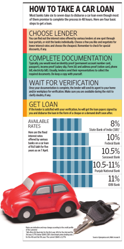

© Copyright 2026