
ESSENTIALS manual. How to effectively detect your (conditional) essential genes... Seq experiment.
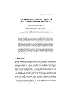
ESSENTIALS manual. How to effectively detect your (conditional) essential genes from a TnSeq experiment.
Summary: We present EssenTials (Essential gene detection by Transposon sequencing), an easy to
use web-interface and an open source software tool for determining conditionally essential genes from
Tn-Seq derived next-generation sequencing data. It features different normalization methods,
statistical tests, genomic location bias correction and visualization options. We successfully applied it
to in-house and published Tn-Seq, INseq, TraDIS and HITS datasets. GSF performs equally well or
better in detecting the conditionally essential genes of literature datasets showing concordance with
previously detected conditionally essential genes and experimental data of gene essentiality.
Availability:
The webinterface of GSF and the example files are freely accessible at:
http://bamics.cmbi.ru.nl/websoftware/essentials/
Contact: [email protected]
1
Table of Contents
Table of Contents .................................................................................................................................... 2 1 Introduction ..................................................................................................................................... 3 2 Part 1. Running the program ........................................................................................................... 4 2.1 Running the software............................................................................................................... 4 2.2 Creating configuration files. .................................................................................................... 5 2.3 Parameter selection.................................................................................................................. 6 3 Run diagnostics ............................................................................................................................. 12 4 Output generated by ESSENTIALS .............................................................................................. 13 4.1 Conditionally essential genes ................................................................................................ 13 4.2 Conditionally essential insertion sites ................................................................................... 18 4.3 Essential genes ...................................................................................................................... 19 5 MINOMICS .................................................................................................................................. 20 5.1 Entering (conditional) gene essentiality data in the database ................................................ 20 5.2 Entering (conditional) insertion site essentiality data in the database. .................................. 22 5.3 Visualizing all data on gene essentiality ............................................................................... 23 2
1
Introduction
Essentials was developed to aid us in our analysis of TN-Seq datasets. Tn-Seq utilizes genome-wide
transposon mutant libraries, of which the presence of each mutant is determined by amplification of
DNA flanking transposon insertions and massively parallel sequencing. Results are mapped on the
genome and summarized for each insertion and gene, generating a measurement of fitness for every
knockout in comparison to the expected values based on the library size and number of insertion sites
per gene.
Similarly, to identify conditionally essential genes, these libraries are exposed to a challenge
condition that will induce lost of mutants of genes essential for survival in these conditions. A
measurement of fitness for every knockout comparison the challenge to the control condition can then
be calculated.
We’ve successfully applied our tool to analyze datasets from Tn-Seq experiments on various
species of S. pneumoniae, H. influenzae and M. catarrhalis in house, but also on literature data sets of
H. influenzae, P. aeruginosa, S. typhi and S. pneumoniae which were generated by Tn-Seq or Tn-seq
like techniques.
Essentials is implemented in Perl and R. Its web-interface is generated by the FG-web framework
(van Hijum et al., unpublished; https://trac.nbic.nl/fgweb/). There are three major sections in the webinterface: (i) configuration file upload and genome selection; (ii) parameter settings; and (iii)
displaying the results. The web tool works with major web browsers such as Internet Explorer,
Firefox, Safari and Opera. It can be tuned to the needs of a researcher by modifying several parameters
controlling the alignments, normalization, statistical tests and visualization.
3
2
Part 1. Running the program
2.1 Running the software
The software is part of the FG-web framework, a bioinformatics work flow system for web based
tools.
Go to http://bamics2.cmbi.ru.nl/websoftware/essentials/essentials_start.php and select your genome of
interest or select your own genbank on your computer.
Select if you want to fill in the sample details manually, or if you want to upload a configuration file
(e.g. from a previous run). Details on editing this file is given in 2.2.
If you want to use the demo reads, just select demo mode and data from our lab on Streptococcus
pneumoniae R6 is used in which a single library was sequenced four times under normal conditions .
The configuration file and the genbank for the demo mode can also be downloaded from this site.
ESSENTIALS has the ability to use premapped reads, either through BAM or SAM files, or through
the use of a tab delimited file, which should look like:
Genomic position<tab>number of reads
Example:
44
809
1279
534
44
211
Figure 1. First page of Essentials webinterface
4
2.2 Creating configuration files.
Although it is possible to fill in the sample characteristics in the website, this can get quite tedious if a
very large number of samples have to be analysed. An alternative is to create the configuration file
manually.
Create a “configuration file” which contains the links to the files containing the samples, the barcodes,
the presence of a transposon sequence, whether they are target or control samples, whether you used
different libraries (for pairwise comparisons), the file format and the compression. The file is tab
delimited. I prefer to use Microsoft Excel (see Figure 1).
•
•
•
•
•
•
•
Create one 1ine per sample. Use the same link to a file if multiple samples are present in the
file.
Barcodes can be of different lengths. If you did not use barcodes, please fill in “N”. This will
assign the entire file to a single sample.
If there is transposon sequence that needs to be removed, please fill in here. Use the sequence
as in the sequence reads, don’t reverse complement etc. If there’s no transposon sequence
present in your reads, fill in “N”.
Sampletype can either be “control”, “target” or “ignore”
If you used a single library, just fill in “lib1” or “library1” etc. If you used multiple libraries
for target and control and you want to do pairwise comparisons, couple the target and control
samples by giving the libraries the same name. Don’t use numbers only for naming the
libraries.
Sampleformat can be “fasta”, “fastq”, “scarf”, “export”, “csfasta” (SOLiD color space fasta),
sam, bam and a custom wiggle tract format “wiggle”.
Compression can be “gz” (gzipped), “bz2” (bzipped) or “zip” (normal zip). Password
protected archives are not supported. Compressed files are expected to contain only one single
file containing the (barcoded) reads.
Save the file as a tab delimited text file.
Figure 2. Configuration file in Microsoft Excel
5
2.3 Parameter selection
Now we’ve arrived at one most important pages in the webinterface, what parameters to select (Fig 3).
Quite some settings can be adapted to suit the experiment. The link “Help, all these settings, what
should I change” gives a concise overview of all the options, but below we will give a more detailed
explanation on the why and how of these settings.
Transposon insertion site options
Selection of librarysize and type of mutagenesis system
Figure 3. Parameter selection
1. Select what kind of integration system was used. Mariner inserts into TA inverted repeat
sequences and upon insertion generates a duplication of the TA site. We can use this to assign
the reads to these specific insertion sites. If you used Tn5 or another method that integrates
randomly, select random. If a new preference site needs to be added for your mutagenesis
system, please contact the authors.
2. The setting library size allows the filtering of spurious reads which could be a common source
of error with Tn-Seq experiments. The insertion sites are sorted according to their number of
reads. When a mutant library of 30k mutants is selected, any data of insertion site 30.0001 and
higher is removed. This filtering is particularly important when no transposon sequence or TA
site is present in your sequence reads, which allows the filtering of actual transposon insertion
reads from spurious reads.
6
Filtering, splitting and alignment options
This section is used to modify the alignments of your read to your reference.
Figure 4. Parameter selection
1. We can select if we want to ignore insertion sites that are not unique. This is recommended,
else insertion sites will be detected and their associated reads will be counted in essential
genes, just because a non-unique piece of DNA was present in the essential gene.
2. The number of mismatches to your barcode can be selected. We use a modified version of the
fastx barcode splitter. The splitter uses Levenshtein (edit) distances instead of hamming
distances to allow for insertions/deletions in barcodes and barcodes of unequal size. Only go
above 2 if you have very large barcodes.
3. Please select how much sequence is left after removal of the barcode and removal of the
transposon sequence.
4. Select on which end the barcode is present. Although commonly on the 5’ end, we cannot rule
out the possibility that someone sequences from the 3’ end but has their barcode on the 5’ end.
5. Select on which end the transposon sequence is (or was!) present. This is quite important,
since this defines what strand was sequenced relative to the transposon cassette. For most TnSeq experiments, the transposon sequence is on the end of the line (3’) which means that you
should also select the reverse strand, instead of the forward strand. For TraDIS for instance,
the transposon sequence is/was present on the 5’ end, resulting in reads on the forward strand
relative to the transposon cassette.
7
6. Select how much sequence triggers a sequence read count in an alignment. The number should
be lower or the same to the number given in step 3.
7. Select what strand to align with. For 5’ (bol) transposon sequence select 0, for 3’ (eol)
transposon sequence select 1 (see 5). If you don’t know (for instance for lit. data), you can
select 2. Settings 5 and 7 determine which side of the read determines the exact insertion site.
8. Select if you want to ignore insertion sites very close to the end of the gene, since these likely
do not cause a loss of functionality. Specifically in the case of mariner which integrates in the
TA insertion and duplicates the TA site. Integration in a TAA stopcodon occurs, the
duplication restores the TAA stopcodon and the transposon insertion, although still detected as
being inside the gene, will not change the gene.
Normalization and statistics options
These settings control several options used in the various R scripts for bias correction, normalization
and statistics.
Figure 5. Parameter selection
1. Presumably, because of genomic replication during growth and the resulting increase in available
DNA close to the origin of replication (ORI), read counts and number of insertions are higher
closer to the ORI, producing a bias in sequencing coverage of insertion sites. We correct for this
bias by using locally weighted scatterplot smoothing (LOESS) on read counts per insertion site to
genomic position. Without this correction, more reads will be found for genes close to the ORI,
potentially causing these to be detected as non-essential when comparing it to the expected
number of reads. This bias can easily cause a 3 fold difference in sequence reads, which could for
8
instance change the ratio between observed and expected read counts from 10 fold to 30 fold.
Consequently, close to the terminus, non-essential genes could be detected as being essential
because of their perceived lower number of reads compared to what is expected.
Reads per insertion site
Reads per gene
X – axis: genomic position
Y – axis log 10 read counts
Figuur 6 A. Bacterial replication. Unlike eukaryotic DNA replication, bacterial replication occurs at one position on
the genome, the origin of replication (ORI) and often multiple replication forks are present in fast dividing cells.
B. Effect of Loess correction. Top: uncorrected, Bottom: corrected. Up 3 fold difference in average read counts can be
seen between insertional positions close to the ORI and close to the terminus.
2. Which normalization to use, TMM, RLE, Quantile or just correction on the total read count per
sample. TMM and RLE are robust methods normally used for RNA-seq data, Quantile is the well
known microarray normalization method from Bolstadt.
3. qCML or CR. The statistical model EdgeR uses is based on the negative binomial distribution.
When a negative binomial model is fitted, we need to estimate the dispersion(s) before we carry
out the analysis. edgeR provides two ways of estimating the dispersion(s), the quantile-adjusted
conditional maximum likelihood (qCML) method and the Cox-Reid profile-adjusted likelyhood
(CR) method. Since the exact test used in the qCML method does not allow the use of
confounders EdgeR uses a Generalized Linear Model to model variances if multiple conditions are
used. In general, we apply the qCML method to experiments with single factor (two conditions,
one single mutant library) and the CR method to experiments with multiple factors (two
conditions, multiple mutant libraries).
4. Common or tagwise dispersion. This parameter controls how the variance is modeled. Common
dispersion means that the same dispersion is used for each gene while moderated tagwise
dispersion allows the use of different dispersion values per gene. Moderated tagwise dispersion
includes the variance in your replicates of each gene per gene, while common only includes the
variance between your replicates between all genes.
5. Prior.n . The value for prior.n determines the amount of smoothing of tagwise dispersions towards
the common dispersion. Quoted from one of the EdgeR developers: “You can think of it as like a
weight for the common value. (It is actually the weight for the common likelihood in the weighted
likelihood equation). The larger the value for prior.n, the more smoothing, i.e. the closer your
tagwise dispersion estimates will be to the common dispersion. If you use a prior.n of 1, then that
gives the common likelihood the weight of one observation”
6. P value adjustment method. The adjustment methods include the Bonferroni correction
(bonferroni) in which the p-values are multiplied by the number of comparisons. Less conservative
corrections are also included by Holm (1979) (holm), Hochberg (1988) (hochberg), Hommel
(1988) (hommel), Benjamini & Hochberg (1995) (BH), and Benjamini & Yekutieli (2001) (BY),
respectively. A pass-through option (none) is also included
9
Minomics visualization option
Figuur 7 Parameter selection
Controls which P value is shown in the info box in the visualization and how many reads will
trigger the generation of the visualization of an insertion site.
Figure 8. Minomics visualization example
10
Other options
Figure 9. Minomics visualization example
Modifies output for debug purposes. At present a zip archive of the results can be generated for quick
download and archival. Additionally an email address can be provided which will be used to report on
the progress of the run.
Press proceed when done.
11
3
Run diagnostics
Steps of the procedure are shown in the running window. This page can be bookmarked and retrieved
at a later stage when the results are ready. Results take between 15 minutes to a couple of hours to
complete. Mostly depends on the speed of download of the sequence files and the size of the genome.
Various statistics are displayed such as the numbers of reads in the file, reads after splitting, reads after
filtering, reads aligned to insertion sites etc.
If there’s a problem with your files, likely it will be shown here. Please contact me
([email protected]) or Sacha van Hijum ([email protected] ) with the link to the failed
analysis on FG-web.
Figure 10. Run diagnostics
12
4
Output generated by ESSENTIALS
Here, we describe the output that can be obtained from an ESSENTIALS run. Various files are
presented to the user, as well as an option to store and visualize the results in MINOMICS, the
genomics visualization tool available in FG-web. Parameters, run log and the original configuration
file containing the download links can also be viewed.
4.1 Conditionally essential genes
If there were target and control samples present, various graphs and a tab delimited table are generated
on gene conditional essentiality. Click on the appropriate links to show them.
Figure 11. Output page
13
PCA plots.
A PCA visualization to discover if the replicates of your datasets are comparable. PCA needs at least
three samples. If only two samples were provided, an x-plot of the samples is produced instead. This
will allow for some comparison between the samples.
Figure 12. Example of a PCA plot with 12 samples. Numbers that are close to each other are samples with similar
data characteristics. In grey the locustags or insertion sites plotted on the same axis.
14
MA plots.
A standard MA plot is produced. The signal is calculated as the log fraction of the number of reads of
a gene divided by the total number of reads. Fold change (y-axis) is the log2 of the number of reads of
the target sample divided by the number of reads of the control sample
Figure 13. Example MA plot. The blue line shows where the log2 2fold change is and genes marked in red are the top
200 significant genes.
Density plot
The log2 transformed ratio of target over control or measured over expected and signal of
(conditionally) essential genes or insertion sites is then used to generate kernel density plots using a
Gaussian model with stepwise increasing bandwidth and 2048 bins until a single (in the case of
essential genes) or four (in the case of conditional essential genes) local minima are found. Local
minima are detected by calculating the first derivative of the density and by locating the position
where it traverses from values below to values above zero. This fold change value corresponds to a
value closest to the minimum between the peaks of essential and non-essential genes and can be used
as a cut-off to determine whether a gene is essential or not.
15
Figure 14. Example density plot. the red dot depics the optimal cutoff point between essential and non-essential genes
Combined table
A table is produced containing the data before between-sample
normalization, after between-sample normalization ,output from
the statistical test and annotation of the genes. This file can be
opened in Microsoft Excel or any other useful utility to read tab
delimited files.
16
Figure 15. Tab delimited conditional gene essentiality output file opened in Microsoft Excel. Column B contains the
locus tags, columns marked with .x contain the data before between-sample normalization. Columns marked with .y
contains data normalized (pseudocounts). The next four columns contain data generated by the statistical test.
logConc: The signal calculated as the log fraction of the number of reads of a gene divided by the total number of
reads, logFC: log2 of the number of reads of the target sample divided by the number of reads of the control sample.
P-value: probability of obtaining a test statistic as the one that was actually observed. Adj. P val: P value adjusted for
multiple testing. The final seven columns contain information about the location, size and annotation of the gene.
Genes marked with NA have less than 10 reads per sample assigned to them either because they are essential, because
they are not hit in the mutant library, or because the gene has no unique insertion sites.
17
4.2 Conditionally essential insertion sites
If there were target and control samples present, various graphs and a tab delimited table are generated
on insertion site conditional essentiality. Click on the appropriate links to show them.
Please see 4.1 for an explanation of the output generated.
Figure 16 Tab delimited conditional insertion site essentiality output file opened in Microsoft Excel. Column C
contains the positions of the insertion sites, columns marked with .x contain the data before between-sample
normalization. Column marked with .y contains data normalized (pseudocounts). The next four columns contain data
generated by the statistical test. logConc: The signal calculated as the log fraction of the number of reads of a gene
divided by the total number of reads, logFC: log2 of the number of reads of the target sample divided by the number
of reads of the control sample. P-value: probability of obtaining a test statistic as the one that was actually observed.
Adj. P val: P value adjusted for multiple testing. The final eight columns contain information about the location, size
and annotation of the gene
18
4.3 Essential genes
Finally, the last section contains information about genes that are always essential. Predictions are
made based on comparison of the expected number of reads of a gene vs the measured number of
reads per gene. The expected number of reads is based on number of (unique) insertion sites in a gene,
the total number of insertion sites in the genome and the number of reads in the sequencing library.
All the outputs are the same as for the conditionally essential genes (see 4.1), except that the final .x
column contains the number of putative insertion sites, the final .y column contains the expected
number of reads.
Figure 1. Tab delimited conditional gene essentiality output file opened in Microsoft Excel. Column B contains the
locus tags, columns marked with .x contain the data before between-sample normalization. The final .x column
contains the number of unique insertion site flanking sequences. Column marked with .y contain data normalized
(pseudocounts). The final .y column contains the expected number of reads. The next four columns contain data
generated by the statistical test. logConc: The signal calculated as the log fraction of the number of reads of a gene
divided by the total number of reads, logFC: log2 of the number of reads of the target sample divided by the number
of reads of the control sample. P-value: probability of obtaining a test statistic as the one that was actually observed.
Adj. P val: P value adjusted for multiple testing. The final seven columns contain information about the location, size
and annotation of the gene. Genes marked with NA have less than 2 reads per sample and less than 2 insertion sites
assigned to them because the gene has no unique insertion sites or because the gene is very small.
19
5
MINOMICS
The data on gene essentiality can be visualized in MINOMICS, a genomics visualization tool
developed by Rutger Brouwer. For more information about MINOMICS, please see
http://bioinformatics.biol.rug.nl/supplementary/minomics/main.php or the journal publication.
MINOMICS relies on count or expression data entered into the Add-2-DB database used in FG-web.
5.1
Entering (conditional) gene essentiality data in the database
To visualize data in MINOMICS, it has to be entered into the database from which the images are
generated. Please follow the steps outlined below
1. Press the purple arrow on the black circle to add data about (conditional) gene essentiality.
If you have not selected an organism for minomics during this session, the organism
selection window will open before data can be added.
2. In the window that opens, select new organism if the organism has not been entered in the
database yet.
20
3. Select the organism of choice and give it a short name. Click proceed. After finishing
close the window.
4. Click on the purple arrow on the black circle again. Now you should be able to add data to
the organism of choice. Select “new” and give the database a description. Press proceed in
the next window
21
5.2 Entering (conditional) insertion site essentiality data in the database.
To visualize insertion site flanking sequences, please follow the steps below:
1. Click on the purple arrow in the black circle in the conditional essential insertion site section
for control insertion sites
2. Add the control insertion sites as regulatory motifs. Use a new database. Name it “control”.
Click proceed, close the next window.
3. Click on the purple arrow in the black circle in the conditional essential insertion site section
for target insertion sites. Add the control insertion sites as regulatory motifs. Use a new
database. Name it “target”. Click proceed, close the next window.
22
5.3 Visualizing all data on gene essentiality
1. Click on Run MINOMICS
2. Click proceed to MINOMICS. We don’t need to upload files since we entered them in the
database already in the previous steps
23
3. Select ratio/P, select the uploaded runs, select operons, motif data, select target and control,
select transcriptional terminators. Click proceed
4. Select if you want to visualize both essential and conditionally essential genes. Click proceed
5. Click proceed in the next window
6. Click proceed in the correlation window. Currently there is nothing to correlate.
24
7. Press genome map in the output window of MINOMICS. A visualization window will open.
The visualization uses SVG and javascript. Please have both enabled. The tool works best in
Firefox. For more information about MINOMICS please visit
http://bioinformatics.biol.rug.nl/supplementary/minomics/main.php
25


© Copyright 2026