How to Strongly Link Data and its Medium:
– the Paper Case –
Philippe Bulens∗, Fran¸cois-Xavier Standaert†,
and Jean-Jacques Quisquater
Universit´e catholique de Louvain, B-1348 Louvain-la-Neuve.
Abstract
Establishing a strong link between the paper medium and the data
represented on it is an interesting alternative to defeat unauthorized copy
and content modification attempts. Many applications would benefit from
it, such as show tickets, contracts, banknotes or medical prescripts. In
this paper, we present a low cost solution that establishes such a link by
combining digital signatures, physically unclonable functions [12, 13] and
fuzzy extractors [7]. The proposed protocol provides two levels of security
that can be used according to the time available for verifying the signature
and the trust in the paper holder. In practice, our solution uses ultraviolet fibers that are poured into the paper mixture. Fuzzy extractors are
then used to build identifiers for each sheet of paper and a digital signature is applied to the combination of these identifiers and the data to be
protected from copy and modification. We additionally provide a careful
statistical analysis of the robustness and amount of randomness reached
by our extractors. We conclude that identifiers of 72 bits can be derived,
which is assumed to be sufficient for the proposed application. However,
more randomness, robustness and unclonability could be obtained at the
cost of a more expensive process, keeping exactly the same methodology.
1
Introduction
Securing documents is an important topic in our everyday life. Bank notes
are probably the most obvious example and it is straightforward to detect, e.g.
micro-printing, ultra-violet inks, . . . that are aimed to make their falsification
difficult. But in fact, many other documents are concerned, e.g. show tickets,
legal papers or medical prescripts. Even the passports that now embed an
RFID chip are still enhanced with such physical protections of which the goal
is to prevent counterfeiting. In other words, they aim to render the effort for
producing good-looking fakes prohibitively high. In general, any field where the
authenticity of a document is important would benefit from a way to prevent
duplication and/or modification. But in practice, the cost of the proposed
solutions also have to be traded with the security level that has to be reached.
∗ Supported
† Associate
by Walloon Region, Belgium / First Europe Program.
researcher of the Belgian Fund for Scientific Research (FNRS - F.R.S.)
1
As a matter of fact, the topic of anti-counterfeiting techniques is very broad.
Even when restricting the concern to paper documents, various contributions
can be found in the scientific literature and in products of companies. For example, Laser Surface Authentication (LSA) extracts a unique fingerprint from almost any document and packaging, based on intrinsically occurring randomness
measured at microscopic level using a laser diode, lenses and photodetectors [3].
The scheme is shown to be highly resistant to manipulation. Moreover, the authors of [8] suggest that the fingerprint could be stored on the document itself
through an encrypted or digitally signed 2D barcode or a smart chip. Another
approach to fingerprint paper is presented in [4]. Using a standard scanner and
by capturing a sheet of paper under 4 different orientations, authors are able to
estimate the shape of the papers’ surface. A unique fingerprint is derived from
those captured physical features which is shown to be secure and robust to harsh
handling. Similarly, printed papers can be authenticated using the inherent nonrepeatable randomness from a printing process [21]. Here, the misplacement of
toner powder gives rise to a print signature that is experimentally shown to be
unique and random. It is then explained how to exploit such a print signature
in order to design a scheme ensuring the authentication of a document.
A similar idea is developed in this paper, i.e. we aim to bind the fingerprint of the medium and the data lying on it. Like in the print signature, this
idea is achieved by performing a digital signature on these information as a
whole. But contrary to [21] where the fingerprint is printed on the paper and
analyzed using shape matching methods (a well-studied problem in computer
vision), we make the fingerprint intrinsic to the paper. For this purpose, we
incorporate ultra-violet fibers during the fabrication process of the paper. The
proposed solution relies on the combination of a Physically Unclonable Function
(PUF) with robust cryptography and randomness extraction schemes. That is,
we use fuzzy extractors to build unique identifiers from the fiber-enhanced papers. Importantly, we mention that using fibers as a PUF was motivated by
low-cost applications (e.g. medical prescriptions, typically). Hence, the actual
unclonability of the proposal is only conjectured for low-cost adversaries. But
increasing the unclonability by considering more complex physical sources of
randomness would be feasible at the cost of a more expensive process (techniques such as presented in [4] could typically be used in this way).
Summarizing, the following results mainly aim to evaluate a coherent application of existing techniques. Additionally to the description of our protocol
for copy or modification detection, we pay a particular attention to the careful
statistical analysis of the robustness and amount of randomness that are extracted from the papers. We believe that such an analysis is interesting since
most published works on PUFs (e.g. based on microelectronic devices [14]) are
limited in the number of samples they use for their estimations.
Note that from a theoretical point of view, such a Sign(content, container)
scheme could be applied to any object. To make it practical only requires a way
to robustly measure the intrinsic features of a medium and to embed a digital
signature. But such an adaptation should also be considered with care since each
ingredient of the protocol could be tuned in function of the target application.
In other words, the solution we propose is general, but finding the best tradeoff
between cost and security for a given application is out of our scope.
2
The rest of the paper is organized as follows. Section 2 gives a global overview
of the proposed method and points out its requirements. The ingredients of our
protocol are described in Section 3. The main contribution of the paper is
then presented in Section 4 in which the paper case study is investigated and
evaluated. Eventually, conclusions are given in Section 5.
2
Overview
In this section, a general overview of the process that we propose for paper
authentication is sketched. The components of the scheme will be discussed
afterwards. First, the signature of a document works as follows.
1. Some additional agent is poured into the paper paste to make secure sheets
(Fig. 1). For example, we use ultra-violet fibers in our application.
2. The physical features of the paper are then extracted, encoded into a tag
T 1, and printed on the paper to authenticate (Fig. 2).
3. Some actual content is printed on the paper (Fig. 3).
4. Eventually, this content is concatenated to the physical information and
signed. The digital signature is encoded in a second tag, T 2 (Fig. 4).
Figure 1: Making paper.
Figure 2: Extracting physical features.
Figure 3: Adding content.
Figure 4: Signing container + content.
3
Second, in order to check if the document is a genuine one, two levels of
security can be considered. These two level are neither mandatory nor exclusive.
Whether one of them or both should be used is driven by the application. For
example, in the context of medical prescription, the pharmacist may decide to
apply the first level of security for his usual customers and the second level for
a person he has never seen before. The verification works as follows.
Level 1. The verifier trusts the second step of the previous procedure and only
performs the verification of the digital signature using T 1, T 2 and the
content of the document (Fig. 5). Interestingly, this process does not
necessarily requires the use of optical character recognition since the paper
content might have been summarized in T 2. Of course, this implies that
the paper content fits into the tag size constraints.
Level 2. A full verification is performed (Fig 6).
1. The physical features of the medium are extracted and encoded in a
new tag T ∗ . This tag T ∗ is then compared with T 1 and the document
is rejected if the two tags do not match.
2. If both tags do match, then the verification proceeds like before.
Using T ∗ or T 1 makes no difference at this stage.
Figure 5: Verification when the owner
of the document is trusted.
3
Figure 6: Full verification with extraction of the medium’s physical features.
Ingredients
To be implemented in practice, the previous authentication process requires different ingredients, namely a digital signature algorithm, a tag encoder/decoder,
a physical unclonable function (PUF) and an extraction scheme. Proposals for
each of those ingredients are discussed in the present section. We mention that
these choices are not expected to be optimal but to provide a solution that
reasonably fits to the low cost requirements of our target applications. Hence,
they could be improved or tuned for other applications.
4
3.1
Signature
Digital signature is a well studied field in cryptography and a variety of solutions
are available for different applications. When devising a real application, using
a standard is a natural way to go. For this reason, the Elliptic Curve Digital
Signature Algorithm (ECDSA [1]) was chosen. Because it provides relatively
short signatures, this lets space for possible addition of content to the tag.
3.2
Tag En-/De- coding
As for digital signature, a large number of visual codes exist, from the old bar
code to more complex 2-dimensional codes. A list of commonly used 2D bar
codes is available on the web [16]. The Datamatrix [9] was chosen for its high
density within a small area (up 1500 bytes in a single symbol whose size can
reduce to a bit more than a 1-inch square with a 600 dpi printer, see Fig. 7).
Figure 7: A datamatrix encodes large amount of data in small areas.
3.3
PUF: Physical Unclonable Function
PUF or equivalently physical one-way functions were introduced by Pappu [12,
13] in 2001. A PUF is an object whose function can easily be computed but is
hard to invert. For a more in-depth view of PUF and their use in cryptography,
we refer to Pim Tuyls et al.’s book [15]. As it will be used in this paper, every
challenge sent to a PUF (i.e. each time a given sheet of paper is scanned)
should be answered by almost the same response (i.e. picture). It should then
be ensured that the size of the response set is large enough to prevent collisions
(i.e. different sheets of paper should not output the same response). Also,
the protected papers should be hard enough to clone. With this respect, PUF
generally rely on some theoretical arguments borrowed from physics.
In our case and as mentioned in the introduction of this paper, we consider
a weaker type of PUF that is just expected to be hard to clone by a low-cost
adversary. According to the papermaker [2], systematically generating twins of
fiber-enhanced papers is an expensive process. But there is still the option for an
attacker to scan the sheet of paper under ultra-violet illumination and attempt
to carefully reproduce the fibers on a clear sheet of paper. This is exactly what
we assumed to be hard enough to be considered as a real threat in our context.
We mention again that the focus of this paper is not in finding the best PUF
but in devising a complete solution for preventing paper modification and copy
and evaluating its reliability in terms of randomness and robustness.
5
3.4
Physical Extraction
The major problem when extracting fingerprints from physical objects is that
they are usually not usable for cryptographic purposes. This difficulty arises
from the fact that (1) the extracted fingerprint may not be perfectly reproduced,
due to small variations in the measurement setup or in the physical source and
(2) the extracted fingerprints from a set of similar objects may not produce the
uniform distributions required by cryptography. Hopefully, turning noisy physical information into cryptographic keys can be achieved using fuzzy extractors.
3.4.1
Theory
The idea of fuzzy extractors arose from the need to deal with noisy data. Therefore, the building parts were somehow spread throughout the literature until
Dodis et al. [7] gathered them all into a general and unified theory. Instead
of devising with fuzzy extractors immediately, the notion of secure sketches is
introduced. A secure sketch is a pair of functionalities: sketch and recover.
First, upon input t, sketch outputs a string s. Then, when recover receives
input t0 and the sketch-computed s, it outputs t provided t0 is close enough
to t. The required property that t remains largely unknown even though s is
available ensures the security of the sketch. The main result of [7] is to prove
that (and show how) fuzzy extractors can be built from secure sketches using
strong randomness extractors. The fuzzy extractor builds upon secure sketches
as depicted in Fig. 8. In an enrollment phase, the input to the sketch procedure
is also sent to a strong extractor, together with randomness u, which generates
output R. The pair (u, s) is stored as data helper, W . Then, in a reconstruction
phase, the data helper is used to regenerate the output R from a new input t0
through recover and extract. In practice, the construction of secure sketches
requires a metric to quantify closeness, e.g. hamming distance, set difference or
edit distance. An example using the hamming distance metric is discussed next.
Enrollment
r
t
u
sketch
extract
Reconstruction
u
u
s }W {s
t’
recover
extract
R
t
R
Figure 8: Turning a secure sketch into a fuzzy extractor.
3.4.2
Practice
In this section, an overview of the practical appraoch developed by Tuyls et
al. [14] is given. The same approach will be used for the paper case. Their
article deals with proof-read hardware, i.e. a piece of hardware within which the
key is not stored but is regenerated when needed. In order to achieve this, two
additional layers are placed on the top of an integrated circuit. The first one is a
grid of capacitive sensors and the second one is an opaque coating containing two
kinds of dielectric particles. The capacitances of this coating are characterized
both across the set of built chips and within a set of measures for the same
6
chip in order to approximate their inter- and intra-class distributions (that are
generally assumed to be Gaussian). Comparing the standard deviations of these
distributions (as in Fig. 9) already gives an intuitive insight on the feasibility
to discriminate different chips. The fuzzy extractor then works as theoretically
described in the previous section: an enrollment is performed once to compute
the extracted fingerprint and its data helper; then reconstruction is performed
any time the key is needed. The global scheme is depicted in Fig. 11.
0.5
0.45
µ2
0.4
Ck
0.35
W
0.3
σ2
0.25
Ck0
X
0.2
Y
0.15
µ1
0.1
σ1
0.05
0
−10
−5
0
5
10
15
20
Figure 9: Comparing the capacitance
inter- and intra-class distributions.
Figure 10: Using the data helper W to
recover a key from a measurement.
During the enrollment phase (left part of Fig. 11), all sensors on a chip
measure the local capacitance of the coating. A first part of the data helper,
denoted as w*, is built as the shift to center the measures in the interval they
lie in. Those intervals are also used to convert each measured value to a short
sequences of bits. The concatenation of those short sequences, the fingerprint
X is used together with the codeword CK (hiding the key K) to generate the
second part of the data helper, denoted as W = X ⊕ CK .
Enrollment
Reconstruction
w*
Object
measure
w*
center data
binarize
data helpers
X
binarize
Success Rate
of the identifiers
CK
Object
Y
encode
K
measure
store
Entropy
of the fingerprints
RNG
correct data
W
W
C’K
decode
K’
Figure 11: Global view of the scheme: Enrollment and Reconstruction phases.
When reconstructing the key (right part of Fig. 11), each output value of
the sensors is corrected with the first part of the helper data and then mapped
to a short sequence of bits whose concatenation is denoted Y . Provided that
Y is not too far away from X (in the sense of hamming distance), CK can be
recovered by decoding Y ⊕W . As the map between the key K and the codeword
CK is uniquely defined, K is immediately identified by CK (see the right part
of Fig. 10). Hence, K can be regenerated at will without worrying about the
7
measurement variations. But if the measures are too far from the ones used
during the enrollment, K won’t be recovered. And this is exactly the expected
behavior: if the measures are too different, the chips assumed to be attacked
and hence should prevent access to the key. We refer to [14] for more details.
4
The Paper Case
To avoid confusion, it is worth clarifying that in this work, fingerprint denotes
the X or Y bit string built from the physics (during enrollment or reconstruction), whereas identifier stand for the K bit string generated from a random
source. In Tuyls et al., K is a key that could be used for encryption. In our case,
K is an identifier that can be recovered. This difference will be reminded later.
From the description of previous section, there are three main steps in the
extraction of a fingerprint from random physical measurements, namely the
measurement of the physical feature, the characterization of its probability distribution and the generation of the bit sequences (X or Y ). For the paper case,
the obvious measurement tool is the one mimicking the human eye. The approach that we chose was to slightly modify a scanner by replacing its white tube
by a fluorescent lamp. The measurement that is performed is thus a uv-scan of
the paper sheet outputting a 24-bit color picture. Using image processing techniques, a list of fibers is then established, each of which is described as tuple
containing position, orientation, surface and color (YUV-components). Given
this as input, the characterization of the probability distributions depends on
mainly three parameters that we detail in the rest of this section.
Number of sensors. As described in Fig. 12, a sheet of paper can be divided in different equal-area sub-sheets. By analogy with the previous coating
PUF example, we denote each of those sub-sheets as a sensor. Quite naturally,
one may decide to extract (a lot of) information from a single sensor or (less)
information from several sensors considered separately.
Number of features per sensor. Given one sensor, we can try to measure
different features from its fibers. For example, we could measure the amount of
fibers N , their orientation O, their luminance L or their overall surface S. In
the following, we will consider those four exemplary features.
Number of bins per sensor. Eventually, one has to determine how much
information we try to extract from each sensor and feature, i.e. the number
of bins used to partition the inter-class distributions. It generally results in a
tradeoff between information and robustness. For example, Fig. 13 depicts an
(imaginary) inter-class distribution. This distribution is sliced in 4 in its bottom
part and in 8 in its upper part. These 4-bin and 8-bin strategies will result to
a maximum entropy of 2 or 3 bits of information per sensor and feature. Note
that the short bit sequences attached to each of the bins are the binary strings
of a Gray code (the same way as in [14]), which allow improving the robustness
of the extraction: if one of the sensor is slightly deviating from its enrollment
value, moving the measure from one bin to its neighbor will result in a string
Y that only differs in 1 bit position from the enrollment string X. Hence, such
an error will be easily corrected when decoding.
8
0.1
1
0
0
0
0.09
0 0 0 1 1 1
0 1 1 1 1 0
1 1 0 0 1 1
1
0
0
0.08
1
0.07
2
0.06
0.05
1
3
2
4
1
2
0.04
3
4
0.03
5
6
0.02
7
X Y
0
0
0
1
1
1
1
0
0.01
8
0
Figure 12: Splitting fiber-enhanced
paper in two, four and eight sensors.
−10
−5
0
5
10
15
20
Figure 13: Characterizing the interclass distribution and Gray codes.
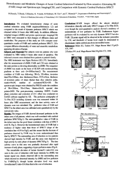
In order to characterize the paper, the whole set of available sheets has been
scanned (1000 different sheets) as well as 16 randomly chosen sheets that were
scanned 100 times. The Lilliefors test was applied to all the samples to check
whether the measurements match a normal distribution, which was actually the
case. As an illustration, the intra- and inter-class distributions of two features
(amount of fibers N and orientation O) are provided in Appendix. Note that
we performed measurements with and without rulers in order to additionally
evaluate the impact of two slightly different setups. A small but noticeable
improvement when using rulers can be seen between the two columns on the
left and the two on the right of the appendix figures (with the exception of the
bottom right picture that represents the inter-class distribution).
4.1
Evaluation Criteria
To evaluate the protocol, two different aspects need to be evaluated: the robustness of the process and the entropy provided by the sheets of secure paper.
Robustness. We first need to ensure that a correctly scanned paper will be
recognized immediately (without requiring additional scan of the same sheet). It
is estimated through the success rate (SR). This later one is simply computed as
the ratio between the amount of correct measures and the amount of measures.
Entropy. We then need to measure the amount of information that can be
extracted from the secure paper. Entropy estimations will be used to evaluate
the number of different fingerprints that we can expect from the process.
4.2
4.2.1
Analysis
Robustness
We first evaluated the success rate, i.e. the robustness, at the output of the
scheme, see Fig. 11. This was done using the 16 sheets that were scanned 100
times. For each of those 16 sheets, the enrollment phase is performed with one of
the scan to build both parts of the data helper. Then, the reconstruction phase
is carried out for the remaining 99 scans. Each time the identifier generated
9
during the enrollment is correctly recovered, it increases the success rate. The
result for the N feature is shown in Fig.14 without error-correcting codes (ECC)
and in Fig. 15 when a BCH(7, 4, 1) code is applied to improve the robustness.
100.00
100.00
100.00
99.37
70.64
95.83
100.00
30.87
54.23
3.22
6.63
0.5
0.06
0.00
3.28
8
0
8
0
17.42
0.57
2.59
2
16
16
0.06
2.71
4
32
32
0.00
8
0.00
8
64
16
4.23
11.30
0.00
0.00
4
44.44
0.5
0.00
0.00
0.00
2
30.49
98.55
1
83.59
Success Rate
Success Rate
1
# sensors
64
16
# bin
# sensors
# bin
Figure 14: Success rate without errorcorrecting codes (N feature).
Figure 15: Success rate with errorcorrecting codes (N feature).
When multiple features and multiple sensors are taken into account, the
fingerprint is built as the concatenation over the sensors of the concatenation
over the features of the Gray codes, namely:
X =kS (kF GC(F, S)) = N
{z } k N
| OLS
{z } k · · · k N
| OLS
{z }
| OLS
S0
S1
SS
The resulting success rate is pictured Fig. 16 and 17, without and with BCH code.
100.00
99.87
99.18
97.10
96.97
89.96
30.81
9.66
1
69.13
Success Rate
Success Rate
1
0.06
1.26
0.5
0.00
0.00
0.06
8
0
16
8
16
0.00
0.00
32
16
32
0.00
8
64
0.00
0.00
0.00
4
0.00
8
0.25
0.25
5.68
0
2
0.00
0.00
4
5.24
11.81
0.00
0.00
0.00
2
83.96
0.5
# sensors
16
# bin
64
# sensors
# bin
Figure 16: Success rate without errorcorrecting codes (4 features).
Figure 17: Success rate with errorcorrecting codes (4 features).
10
Increasing either the number of sensors or the number of bins decreases the
success rate. However, it is also clear that increasing the number of sensors is a
better approach than increasing the number of bins with respect to robustness.
Other parameters for the error-correcting code can be plugged in. For example, Fig. 18 and Fig. 19 use BCH codes able to correct up to 2 and 3 errors,
respectively. In the case of 64 sensors, 2 bins and BCH(31, 16, 3), this improves
the success rate up to 95%, a reasonable target value for real applications.
100.00
100.00
100.00
100.00
48.93
99.43
91.41
1
30.93
10.48
Success Rate
Success Rate
1
0.5
12.88
1.01
2.59
8
0
12.31
0.5
22.03
8
11.05
0.00
0.69
2
16
16
0.00
0.00
4
32
32
0.00
8
0.00
8
64
16
0.82
3.79
0
0.00
0.00
4
36.11
95.52
0.00
0.63
6.57
2
52.90
99.94
# sensors
64
16
# bin
# sensors
# bin
Figure 18: Success rate with ECC:
BCH(15, 7, 2) (4 features).
Figure 19: Success rate with ECC:
BCH(31, 16, 3) (4 features).
Finally, we also evaluated the impact of embedding a ruler in the scanner
to ensure proper positioning of the sheet before scanning. Out of the 16 sheets
scanned 100 times, 6 were scanned after the ruler was setup.
100.00
100.00
100.00
98.69
57.58
100.00
95.15
14.75
100.00
1
74.34
Success Rate
Success Rate
1
0.71
1.62
0.5
0.00
0.00
0.51
8
0
14.31
16
8
16
0.00
0.00
32
16
32
0.00
8
64
0.00
0.00
0.00
4
0.00
8
0.67
0.67
0
2
0.00
0.00
4
12.79
0.5
0.00
0.00
0.00
2
28.79
# sensors
16
# bin
64
# sensors
# bin
Figure 20: Success rate without ruler
(4 features, 10 sheets, BCH(7, 4, 1)).
Figure 21: Success rate with a ruler (4
features, 6 sheets, BCH(7, 4, 1)).
11
The difference already mentioned in the appendix is now easily observed in
Fig. 20 and 21 that have to be compared with Fig.17 where all the sheets have
been evaluated without distinguishing the use (or not) of the ruler.
4.2.2
Entropy
In order to estimate the entropy of the physical source, we used 1000 fingerprints generated as pictured in Fig. 11. We started with a simple sensor-based
approach in which we evaluated the entropy using histograms. We note that
computing the entropy per sensor is meaningful as long as these sensors can be
considered independent. This seems a reasonable physical assumption in our
context. By contrast, it is obviously not a good solution to evaluate the entropy
when exploiting different features that are most likely correlated. Anyway, the
histogram-based approach was just applied for intuition purposes and combined
with the more advanced evaluations described in the end of this section.
0.1
0.1
0.09
0.09
0.08
0.08
0.07
0.07
0.06
0.06
0.05
0.05
0.04
0.04
0.03
0.03
0.02
0.02
0.01
0
0.01
−10
−5
0
5
10
15
0
20
Figure 22: One set to estimate the
distribution and build the bins.
−10
−5
0
5
10
15
20
Figure 23: Each sheet of the second
set is placed in its corresponding bin.
In practice, let us assume a single sensor per sheet and 4 bins per sensor.
We first used 500 scans to determine the positions of the bins as in Fig. 22.
Then, we used the second set of 500 scans to evaluate the probabilities of the
previously determined bins as in Fig. 23. Eventually,
we estimated the entropy
P
per sensor using the classical formula: H = − i pi log pi where the pi are the
bin probabilities. Such a naive method gives the results shown in Fig. 24.
Note that for some choices of parameters, the entropy was stuck to zero.
This is simply because the number of samples was not sufficient to fill all the
bins in those cases. Indeed, given the size of the sample set, one can determine
the amount of bins that should not be crossed to keep meaningful results, e.g.
using Sturges rule1 : d1 + log2 M e, with M the size of the set. In our example, it
states that there should be no more than 10 bins. The entropies stuck to ground
in Fig. 24 can be seen as the limits for the given sample size. Quite naturally,
we see that the informativeness of an extractor increases with the number of
sensors and bins, contrary to its robustness in the previous section.
1 Scott’s
formula gives a similar result:
3.5σ
M 1/3
12
=
3.5·23
5001/3
= 10.146 . . .
124.31
Entropy
150
100
63.62
62.74
46.35
50
30.72
0
31.47
31.16
64
23.04
16
15.56
15.29
32
8
16
7.61
4
8
2
# sensors
# bin
Figure 24: Sensor-based entropy estimation using histograms for the N feature.
In order to confirm these first estimations, we then ran more complex test
suites, in particular: ent [17], Maurer’s test including Coron’s modification [11,
6, 5] and the Context Tree Weighting (CTW) method [18, 19, 20]. The main
idea behind these entropy estimation tools is to compare the length of an input
sequence and its corresponding compressed output. For the details about how
they actually process the data, we refer to the previous links.
These final results achieved are given in table 1, where X(F, S, B) denotes
the fingerprint built upon features F when cutting the paper in S sensors sliced
in B bins. As previously explained, when multiple features and multiple sensors
are involved, the fingerprint is built as the concatenation over the sensors of
the concatenation over the features of the Gray codes, X =kS (kF GC(F, S)).
The first column where fingerprints are only built from the amount of fibers
(N) shows that almost 32 bits of entropy can be extracted from the 32-bit
strings which essentially confirms that different sensors are indeed independent.
By contrast, when using 4 different features as in the right part of the table,
we clearly see that the entropy extracted per bit of fingerprint is reduced, i.e.
the features (amount of fibers, orientation, luminance and surface) are actually
correlated. Most importantly, we see that overall the proposed solution allows
to generate fingerprints with slightly more than 96 bits of entropy while ensuring
a good robustness. In other words, this solutions largely fulfills the goal of a
low-cost authentication process that we target in this paper.
Ent
Maurer*
CTW
X(N, 32, 2)
1 · 32 · 0.99 = 31.68
1 · 32 · 0.99 = 31.68
1 · 32 · 0.99 = 31.68
X(N OLS, 32, 2)
4 · 32 · 0.99 = 126.72
4 · 32 · 0.63 = 80.64
4 · 32 · 0.75 = 96.53
Table 1: Entropy estimations in entropy bits per fingerprint X.
Note finally that our use of fuzzy extractors significantly differs from the one
of Tuyls et al.. We use physical features to build unique (but public) identifiers
while [14] aims to generate cryptographic keys. Therefore, we do not have to
13
evaluate the secrecy of our identifiers but only their randomness. This is because
in our protocol, the overall security comes from the digital signature that is
applied both to the identifiers and to the content printed on a paper. An attack
against our scheme would require to find a sheet of paper that gives the same
identifier to perform a copy/paste attack. This is supposed to be hard enough
in view of the 96 bits of entropy that the physical features assumably provide.
5
Conclusion
In this paper, a proposal to secure documents is presented that combines previously introduced robust cryptographic mechanisms and information extractors
with a source of physical randomness. It has the interesting feature to provide
two levels of verification, trading rapidity for trust. The scheme is quite generic
and could be tuned for different application needs. Our case study was developed
for low-cost standard desktop equipment. But the robustness, randomness and
(mainly) unclonability of our proposal could be improved at the cost of a more
expensive infrastructure. We also provide a detailed and motivated statistical
analysis of the information extraction scheme. In the studied case, embedded
ultra-violet fibers allows extracting 128-bit strings that correspond to an entropy of approximately 96 bits while providing 72-bit identifiers when applying
an error correcting code. The resulting identifiers can be extracted with high
robustness. This is considered to provide a sufficient security since an adversary
would have to scan a prohibitive amount of secure paper to find a collision.
Acknowledgment
The authors would like to thank Nicolas Veyrat-Charvillon for his help while
developing all the tools required during this work and to Fran¸cois Koeune as
well as Giacomo de Meulenaer for the fruitful discussions.
References
[1] American National Standards Institute – ANSI. Public key cryptography
for the financial services industry, the Elliptic Curve Digital Signature Algorithm (ECDSA). ANSI X9.62:2005, 2005.
[2] Arjo Wiggins: Security Division. http://www.security.arjowiggins.com/.
[3] J. D. R. Buchanan, R. P. Cowburn, A.-V. Jausovec, D. Petit, P. Seem,
G. Xiong, D. Atkinson, K. Fenton, D. A. Allwood, and M. T. Bryan. Fingerprinting documents and packages. Nature, 436:475, 2005.
[4] W. Clarkson, T. Weyrich, A. Finkelstein, N. Heninger, J. A. Halderman,
and E. W. Felten. Fingerprinting blank paper using commodity scanners.
Porc. of IEEE Symposium on Security and Privacy, May 2009.
[5] J.-S. Coron. On the security of random sources. Public Key Cryptography
— PKC’99, Lecture Notes in Computer Science 1560:29–42, 1999.
14
[6] J.-S. Coron and D. Naccache. An accurate evaluation of maurer’s universal
test. Selected Areas in Cryptography — SAC’98, Lecture Notes in Computer
Science 1556:57–71, 1998.
[7] Y. Dodis, R. ostrovsky, L. Reyzin, and A. Smith. Fuzzy extractors: How to
generate strong keys from biometrics and other noisy data. SIAM Journal
on Computing, 38(1):97–139, 2008.
[8] Ingenia Technology Ltd. http://www.ingeniatechnology.com.
[9] International Organization for Standardization – ISO. Information technology — International symbology representation — Datamatrix. ISO/IEC
16022:2000(E), 2000.
[10] A. Juels and M. Wattenberg. A fuzzy commitment scheme. Conference on
Computer and Communications Security — CCS’99, Proceedings of the 6th
ACM conference on Computer and communications security:28–36, 1999.
[11] A. J. Menezes, P. C. van Oorschot, and S. A. Vanstone. Handbook of
Applied Cryptography. CRC Press, 2001.
[12] R. Pappu. Physical one-way functions. Ph. D. dissertation, 2001.
[13] R. Pappu, B. Recht, J. Taylor, and N. Gershenfeld. Physical one-way
functions. Science, 297:2026–2030, 2002.
ˇ
[14] P. Tuyls, G. J. Schrijen, B. Skori´
c, J. van Geloven, N. Verhaegh, and
R. Wolters. Read-proof hardware from protective coatings. Cryptographic
Hardware and Embedded Systems — CHES’06, Lecture Notes in Computer
Science 4249:369–383, 2006.
ˇ
[15] P. Tuyls, B. Skori´
c, and T. Kevenaar. Security with Noisy Data: Private
Biometrics, Secure Key Storage and Anti-Counterfeiting. Springer-Verlag
New York, Inc., 2007.
[16] Unibar Inc. Bar code page. http://www.adams1.com/stack.html.
[17] J. Walker. Ent: A pseudorandom number sequence test program.
http://www.fourmilab.ch/random/.
[18] F. Willems. The context-tree weighting method: Extensions. IEEE Transactions on Information Theory, 44:792–798, 1994.
[19] F. Willems, Y. Shtarkov, and T. Tjalkens. Reflections on ”the context-tree
weighting method: Basic properties”.
[20] F. Willems, Y. Shtarkov, and T. Tjalkens. The context-tree weighting
method: Basic properties. IEEE Transactions on Information Theory,
41:653–664, 1995.
[21] B. Zhu, J. Wu, and M. S. Kankanhalli. Print signatures for document
authentication. Conference on Computer and Communications Security,
Proceedings of the 10th ACM conference on Computer and communications
security:145–153, 2003.
15
16
300
320
360
380
400
420
420
300
320
300
320
340
360
380
400
420
340
360
380
400
420
340
360
N − 159
380
400
420
300
320
300
320
340
360
N − 243
300
320
380
400
420
0
280
2
4
6
8
300
320
µ = 407.99
σ = 4.61
10 σ / σ = 4.99
e
a
12
0
280
2
4
6
µ = 374.40
σ = 5.33
8 σe / σa = 4.32
10
0
280
360
340
360
N − 672
340
380
380
400
400
420
420
340
360
N − 796
380
400
420
Figure 25: Intra- and inter-class distributions for the amount of fibers N .
0
280
320
1
2
3
4
5
6
µ = 363.44
8 σ = 7.18
σe / σa = 3.20
7
9
0
280
300
N − 216
1
2
3
4
5
µ = 402.58
7 σ = 8.24
σe / σa = 2.79
6
8
0
280
2
4
6
µ = 349.87
σ = 6.60
8 σe / σa = 3.49
10
0
280
2
N − 566
300
320
4
6
8
10
320
0
280
10
20
30
40
300
320
µ = 355.12
σ = 23.01
50 σ / E(σ ) = 3.53
e
a
60
300
µ = 410.93
12 σ = 5.36
σe / σa = 4.29
14
0
280
1
2
3
4
5
6
µ = 390.03
8 σ = 5.39
σe / σa = 4.27
7
9
0
280
340
400
1
2
4
6
4
3
8
10
µ = 388.42
12 σ = 4.73
σe / σa = 4.87
14
2
320
380
N − 049
5
6
µ = 388.13
8 σ = 7.22
σe / σa = 3.19
7
9
0
280
300
360
N − 138
340
N − 023
1
2
3
4
5
µ = 369.22
6 σ = 8.42
σe / σa = 2.73
7
0
280
2
4
6
µ = 385.51
σ = 8.62
8 σe / σa = 2.67
10
360
360
340
360
N − Inter
340
N − 750
340
N − 612
380
380
380
400
400
400
420
420
420
17
450
600
650
650
700
700
2
3
4
5
6
500
500
500
550
O − 243
550
O − 159
550
O − 049
600
600
600
650
650
650
700
700
700
450
450
0
400
1
2
3
4
450
µ = 652.55
σ = 7.82
5 σ / σ = 5.07
e
a
6
0
400
1
2
3
4
5
µ = 584.10
7 σ = 8.75
σe / σa = 4.53
6
8
0
400
2
4
6
µ = 612.59
σ = 8.21
8 σe / σa = 4.83
10
500
500
500
550
O − 796
550
O − 672
550
O − 566
600
600
600
650
650
650
700
700
700
450
450
500
500
0
400
10
20
30
40
50
450
500
µ = 557.92
60 σ = 39.61
σe / E(σa) = 3.57
70
0
400
1
2
3
4
5
µ = 643.59
7 σ = 9.05
σe / σa = 4.38
6
8
0
400
1
2
3
4
µ = 604.71
σ = 8.20
5 σ / σ = 4.83
e
a
6
Figure 26: Intra- and inter-class distributions for the orientation of the fibers O.
450
0
400
0
400
700
1
1
650
2
2
600
3
3
550
4
4
450
5
5
7
µ = 556.14
6 σ = 12.34
σe / σa = 3.21
500
O − 216
450
µ = 648.83
6 σ = 14.55
σe / σa = 2.72
7
450
µ = 550.82
8 σ = 11.76
σ / σ = 3.37
7 e a
9
0
400
0
400
550
600
0
400
500
O − 138
550
2
4
6
µ = 610.22
σ = 12.66
8 σe / σa = 3.13
10
1
450
500
O − 023
1
2
3
4
5
µ = 577.65
7 σ = 14.17
σe / σa = 2.80
6
8
0
400
1
2
3
4
5
µ = 608.45
7 σ = 14.65
σe / σa = 2.70
6
8
550
O − Inter
550
O − 750
550
O − 612
600
600
600
650
650
650
700
700
700