How to apply SAT-solving for
the equivalence test of monotone normal forms?
Martin Mundhenk and Robert Zeranski
Friedrich-Schiller-Universit¨
at Jena, Germany
{martin.mundhenk, robert.zeranski}@uni-jena.de
Abstract. The equivalence problem for monotone formulae in normal
form Monet is in coNP, is probably not coNP-complete [1], and is solvable in quasi-polynomial time no(log n) [2].
We show that the straightforward reduction from Monet to UnSat
yields instances, on which actual Sat-solvers (SAT4J) are slower than
current implementations of Monet-algorithms [3]. We then improve these
implementations of Monet-algorithms notably, and we investigate which
techniques from Sat-solving are useful for Monet. Finally, we give an advanced reduction from Monet to UnSat that yields instances, on which
the Sat-solvers reach running times, that seem to be magnitudes better
than what is reachable with the current implementations of Monetalgorithms.
1
Introduction
The equivalence problem for Boolean formulae is one of the classical coNP-complete problems. It remains coNP-complete also if the formulae are given in normal
form. For monotone formulae—i.e. formulae with conjunctions and disjunctions,
but without negations—the equivalence problem is coNP-complete, too [4], but
its complexity drops, if the formulae are in conjunctive or disjunctive normal
form. The reason is that for every monotone formula, the minimal equivalent formula in the considered normal form is unique, and the minimal equivalent normal
form formula is efficiently computable from the non-minimal normal form formula. Therefore, checking whether two monotone formulae in conjunctive normal
form (resp. two monotone formulae in disjunctive normal form) are equivalent,
can be done in polynomial time. The remaining case is the equivalence problem
for monotone formulae, where one formula is in conjunctive normal form and the
other is in disjunctive normal form. This is the problem Monet, i.e. Mo(notone)
n(ormal form) e(quivalence) t(est). This problem is strongly related to dualization of monotone conjunctive normal forms and transversal hypergraph generation [5]. This means that an algorithm for Monet solves many fundamental
problems in a wide range of fields, including artificial intelligence and logic, computational biology, database theory, data mining and machine learning, mobile
communication systems, distributed systems, and graph theory (see [3] for an
?
This work was supported by the DFG under grant MU 1226/8-1 (SPP 1307/2).
overview). The currently best Monet algorithms have quasi-polynomial running
time no(log n) , or polynomial time using O(log2 n) nondeterministic bits [6,2,1].
Thus, on the one hand, Monet is probably not coNP-complete, but on the other
hand a polynomial time algorithm is not yet known. This situation turns Monet
into one of the very few problems “between” P and NP- resp. coNP-hard. The
exact complexity of the general problem Monet is a long standing famous open
question [7].
As for evaluating the practical performance, in [8,9,10,11,12,13,14] one can
find several experimental studies on known algorithms for Monet or equivalent
problems. Over all, the algorithms by Fredman and Khachiyan [2], that are the
Monet algorithms with the best worst-case upper-bounds, turn out to be strong
practical performers [3].
In this paper, we mainly address the following two questions.
Can the performance of the algorithms by Fredman and Khachiyan be improved
by using techniques from Sat-solving? The two algorithms by Fredman and
Khachiyan basically use a technique similar to the DPLL-algorithm for Sat [15].
Both algorithms leave—more or less—open which variable to choose as the splitting variable. We added unit propagation and tried several strategies known from
Sat-solving like MOMs [16], BOHM [17], and clause reduction heuristic [18]. In
our experimental study we show that unit propagation and the mentioned strategies notably improve our implementations of the algorithm.
Are Sat-solvers good for Monet? Since Monet reduces to the complement of
Sat, it is straightforward to use a reduction and a Sat-solver to solve Monet.
Eventually, it turned out not to be that straightforward. We give a reduction
from Monet to the complement of Sat that does not increase the size of the
instances. Using this reduction function and a Sat-solvers reaches computation
times that are very much better than what is currently possible with Monet
solvers.
This paper is organized as follows. In Section 2 we introduce the basic notation and review the FK-algorithms [2]. Section 3 shows how unit propagation
and strategies for choosing a splitting variable can be used in the FK-algorithms.
Section 4 considers how Monet can be reduced UnSat. Our experimental results are discussed in Section 5, and conclusions are drawn in Section 6.
2
Preliminaries
Monotone formulae and equivalence A Boolean formula ϕ is called monotone if ϕ has only ∧ and ∨ as connectives–no negations are allowed. Let Vϕ denote
the set of variables of ϕ. An assignment is denoted as a set A ⊆ Vϕ of variables,
where x is assigned true iff x ∈ A. Otherwise x is assigned false. A term is a set
of variables that is either interpreted as a conjunction or as a disjunction of the
variables. We call a term a monomial if it is a conjunction and we call it a clause
if it is a disjunction. In this paper m always denotes a monomial and c always
denotes a clause. A monotone Boolean formula is a DNF (disjunctive normal
form) if it is a disjunction of monomials, and it is a CNF (conjunctive normal
form) if it is a conjunction of clauses. Throughout the whole paper we regard
a CNF (resp. DNF) as a set of clauses (resp. monomials). A monotone DNF or
CNF is called irredundant if it contains no two terms such that one contains the
other. It is important, that every monotone Boolean formula has a unique irredundant monotone CNF and DNF [19]—and for a given monotone CNF (resp.
DNF) the irredundant CNF (resp. DNF) can be obtained in quadratic time by
deleting all supersets of terms. Two monotone Boolean formulae are equivalent
if and only if they have the same irredundant monotone CNF. This paper deals
with the equivalence test of monotone formulae in different normal forms.
Monet:
Instance: irredundant, monotone DNF D and CNF C
Question: are D and C equivalent?
In this paper D always denotes a monotone DNF and C always denotes a
monotone CNF. The length of a term is the number of variables in this term,
and the length of a normal form D (resp. C) is the number of terms in it.
The algorithms of Fredman and Khachyian
The algorithms with the best known worst-case upper bound for solving Monet
are by Fredman and Khachiyan [2]. Both these algorithms search for a witness
of non-equivalence by a depth-first search in the tree of all assignments—we call
such a witness conflict assignment. Note that this technique is very similar to the
DPLL-algorithm for Sat [15]. The FK-algorithms work as follows. In the first
step the input formulae are modified to irredundant normal forms.1 Unless the
formulae are small enough to check them by brute force, the algorithm chooses
a variable, sets the value of this variable to false and modifies the formulae due
to this assignment—we call the variable chosen the splitting variable. Next, the
equivalence of the new formulae will be tested recursively. If the recursive call
does not yield a conflict assignment, the splitting variable is set to true and the
accordingly modified formulae are tested recursively. If this second recursive call
does not yield a conflict assignment, then the formulae must be equivalent.
The modifications of the formulae are as follows. If a variable is set to true
in a DNF, then this variable can be deleted in each monomial. And if it is set to
false, then all terms which contain this variable can be deleted. For the CNF it is
dual. Let φ be a DNF or CNF, and let x be a splitting variable. Then φx0 denotes
the formula that consists of terms of φ from which x is removed. Analogously,
φx1 denotes the formula that consists of all terms of φ that do not contain x.
φx0 = {t − {x} : t ∈ φ and x ∈ t}
φx1 = {t : t ∈ φ and x 6∈ t}
Thus, if x is set to true in D and C, we obtain D0x ∨ D1x and C1x . If it is set to
false, we obtain D1x and C0x ∧ C1x .
Fredman and Khachiyan [2] provide necessary conditions for equivalence,
that are also checked during the depth-first search, as follows.
1
This step is necessary because the formulae will be modified in further steps and the
algorithms are recursive.
(1) m ∩ c 6= ∅ for every monomial m ∈ D and every clause c ∈ C.
(2) D and C must contain exactly the same variables, i.e. VD = VC .
(3) max{|m| : m ∈ D} ≤ |C| and max{|c| : c ∈ C} ≤ |D|.
FK-algorithm A [2] The central question is about the choice of the splitting
variable. Fredman and Khachiyan provide an additional necessary condition for
the FK-algorithm A which ensures the existence of a frequent variable.
X
m∈D
2|VD |−|m| +
X
2|VC |−|c| ≥ 2|VD | .
(4)
c∈C
If this condition is violated the formulae are not equivalent and a conflict
assignment can be computed in linear time. As splitting variable FK-algorithm
A chooses a variable with frequency ≥ 1/ log(|D| + |C|) in either D or C.
Theorem 1. [2] FK-algorithm A has running time nO(log
where n = |D| + |C|.
2
n)
on input (D, C),
Algorithm 1 shows a pseudo-code listing of FK-algorithm A. It is shown in an
experimental study in [10] that FK-algorithm A performs well in practice.
There is also a version presented in [20] which works in space polynomial in
|D|.
FK-algorithm B [2] What happens if the first recursive call FK-A(D1x , C0x ∧
C1x ) of FK-algorithm A does not yield a witness for non-equivalence? In this
case we gain the information that D1x is equivalent to C0x ∧ C1x . FK-algorithm A
does not use the fact that the second recursive call is performed only if the first
recursive call does not yield a witness for non-equivalence. But FK-algorithm B
makes use of this. The main conclusion is a restriction for the search tree when
the value of the splitting variable is set to true. It then suffices to find a conflict
assignment A for the formulae D0x and C1x with the restriction that A(C0x ) = 0
(cf. [2,3]). Hence, one has to check all maximal assignments not satisfying C0x
only. Note that there are exactly |C0x | assignments, one for every clause c ∈ C0x
(the resp. assignment is VC0x − c).
Thus, if the first recursive call does not yield a conflict assignment it suffices
to perform a recursive call for every clause c ∈ C0x on the pair (D0c,x , C1c,x ), where
D0c,x and C1c,x denote the formulae we obtain if we set all variables in c to false.
We receive a similar result if we swap the chronological order of the first and
the second recursive call, cf. [2,3]. If the recursive call on the pair (D0x ∨ D1x , C1x )
does not yield a witness for non-equivalence it suffices to perform a recursive call
for every monomial m ∈ D0x on the pair (D1m,x , C0m,x ), where D1m,x and C0m,x
denote the formulae we obtain if we set all variables in m to true (if we found a
conflict, the resp. assignment is m).
One of the main differences to FK-algorithm A is the choice of the variable and the advanced branching. The choice of the splitting variable does not
matter in [2] for the theoretical upper bound, because FK-algorithm B chooses
Algorithm 1 The FK-algorithm A (FK-A)
Input: irredundant, monotone DNF D and CNF C
Output: ∅ in case of equivalence; otherwise, assignment A with A(D) 6= A(C)
1: make D and C irredundant
2: if one of conditions (1)–(4) is violated then
3:
return conflict assignment
4: if |D| · |C| ≤ 1 then
5:
return appropriate assignment found by a trivial check
6: else
7:
choose a splitting variable x with frequency ≥ 1/ log(|D| + |C|) in D or C
8:
A ← FK-A(D1x , C0x ∧ C1x )
// recursive call for x set to false
9:
if A = ∅ then
10:
A ← FK-A(D0x ∨ D1x , C1x )
// recursive call for x set to true
11:
if A 6= ∅ then return A ∪ {x}
12: return A
Algorithm 2 The FK-algorithm B (FK-B)
Input: irredundant, monotone DNF D and CNF C
Output: ∅ in case of equivalence; otherwise, assignment A with A(D) 6= A(C)
1: make D and C irredundant
2: if one of conditions (1)–(3) is violated then return conflict assignment
3: if min{|D|, |C|} ≤ 2 then
4:
return appropriate assignment found by a trivial check
5: else
6:
choose a splitting variable x from the formulae
7:
if x is at most µ-frequent in D then
8:
A ← FK-B(D1x , C0x ∧ C1x )
// recursive call for x set to false
9:
if A 6= ∅ then return A
10:
for all clauses c ∈ C0x do
11:
A ← FK-B(D0c,x , C1c,x )
// see h1i
12:
if A =
6 ∅ then return A ∪ {x}
13:
else if x is at most µ-frequent in C then
14:
A ← FK-B(D0x ∨ D1x , C1x )
// recursive call for x set to true
15:
if A 6= ∅ then return A ∪ {x}
16:
for all monomials m ∈ D0x do
17:
A ← FK-B(D1m,x , C0m,x )
// see h2i
18:
if A =
6 ∅ then return A ∪ m
19:
else
20:
A ← FK-B(D1x , C0x ∧ C1x )
// recursive call for x set to false
21:
if A = ∅ then
22:
A ← FK-B(D0x ∨ D1x , C1x )
// recursive call for x set to true
23:
if A =
6 ∅ then return A ∪ {x}
24: return A
h1i: D1x ≡ C0x ∧ C1x : recursive call for all maximal non-satisfying assignments of
C0x for x set to true
h2i: D0x ∨ D1x ≡ C1x : recursive call for all minimal satisfying assignments of D0x for
x set to false
an appropriate branching with respect to the frequency of the splitting variable. Therefore, the algorithm uses a frequeny-threshold µ(n) with the property µ(n)µ(n) = n. Note, that µ(n) ∼ log n/ log log n. Thus, µ(n) ∈ o(log n). A
pseudo-code listing of FK-algorithm B is given in Algorithm 2. There, a variable x is called at most µ-frequent in D (resp. C) if its frequency is at most
1/µ(|D| · |C|), i.e. |{m ∈ D : x ∈ m}|/|D| ≤ 1/µ(|D| · |C|).
Theorem 2. [2] FK-algorithm B has running time no(log n) on input (D, C),
where n = |D| + |C|.
3
Unit propagation and decision strategies
As mentioned before, the choice of the splitting variable is free in FK-algorithm
B, and it is almost free in FK-algorithm A. In the old implementations in [3],
the first variable in the formula is taken as splitting variable for FK-algorithm
B, and the first variable that satisfies the frequency condition is taken as splitting variable in FK-algorithm A. In our new implementations, we replaced this
by running unit propagation and choosing a splitting variable according to a
somewhat more involved strategy.
Unit propagation for Monet Unit propagation (UP), or also called oneliteral rule, is a technique for simplifying a set of clauses in an automated theorem
proving system. This technique is also used for the DPLL-algorithm [15]. A
clause (resp. monomial) is a unit clause (resp. unit monomial ) if it consists of
one variable only. How can the FK-algorithms gain from considering unit clauses
or unit monomials? There are two cases.
Case (a): There is a unit clause in C. Let {x} ∈ C, and let D and C satisfy
condition (1). Then C0x –i.e. the set of clauses obtained from CNF C by setting x
to false–is unsatisfiable, and D1x –i.e. the set of monomials obtained from DNF D
by setting x to false–is unsatisfiable, too, because x is contained in all monomials
of D (cf. condition (1)). Thus, the recursive call for setting the splitting variable
x to false will yield no conflict assignment and can be left out.
Lemma 1. Let {x} ∈ C. Then D ≡ C if and only if D1x = ∅ and D0x ≡ C1x .
According to Lemma 1, if C contains a unit clause {x} then it suffices to check
condition (1) on (D0x , C1x ) and to do the recursive call FK-A(D0x , C1x ).
Case (b): There is a unit monomial in D. This case is dual to case (a).
Lemma 2. Let {x} ∈ D. Then D ≡ C if and only if C1x = ∅ and D1x ≡ C0x .
Note, that for formulae D and C satisfying condition (1) it is impossible that
D and C contain the same unit term (excepted D = C = {{x}}). Thus, one
can search for all unit clauses and unit monomials in the formulae and setting
the variables to the resp. values. Because both formulae are irredundant we only
have to delete the unit terms in the resp. formula. If there is no unit term left in
D and C we can choose a splitting variable. It is also possible to avoid checking
condition (1). Thus, if we find a unit term {x} in D (resp. C) we have to check
that x is contained in all terms of C (resp D).
Decision strategies for the splitting variable A main difference between
FK-algorithm A and FK-algorithm B is the choice of the splitting variable.
FK-algorithm A chooses a variable that is at least log(|D| + |C|)-frequent in
either D or C—one can also simply choose the most frequent variable. (If D is
equivalent to C, then there exists a log(|D|+|C|)-frequent variable [2]). However,
FK-algorithm B is free to choose any variable as splitting variable. In general,
a random choice is not a good strategy (see experiments with FKB(rMin) in
Section 5). Thus, it is interesting to investigate whether strategies for choosing
the splitting variable improve FK-algorithm B. We tried the following strategies.
(i)
(ii)
(iii)
(iv)
(v)
(vi)
4
Choose the first free variable [3]—it is related to a random choice.
Choose the most frequent variable.
Choose the most frequent variable in the smallest terms (MOMs [16]).
Choose a variable randomly in the smallest terms.
Choose the variable with maximal occurence in small terms (BOHM [17]).
Clause reduction heuristic (CRH [18]).
Solving Monet using SAT-solvers
Since Monet is in coNP, it is polynomial-time reducible to UnSat. Therefore, a
straightforward approach to solve Monet is to use this reduction and a common
SAT-solver. Clearly, (D, C) is in Monet if and only if ¬(D → C) 6∈ Sat and
¬(C → D) 6∈ Sat.
Since D is a DNF and C is a CNF, the formula ¬(C → D) is represented by
the CNF C∪D¬ , where D¬ is the set of monomials in D, in which all appearances
of variables are negated.2 Similarly, the other part ¬(D → C) can be seen as a
conjunction of two DNFs and can be brought into conjunctive normal form using
the standard translation by Tseitin [21] that results in an equisatisfiable formula
in CNF. Even though this translation enlarges the formula only linearly, our
experiments with SAT-solvers on the translated formulae yielded computation
times that were worse than that of the FK-algorithms (see Section 5, Table 2).
Let us consider the formula ¬(D → C) more precisely. It is satisfied by
assignments that satisfy a monomial in the DNF D and falsify all clauses in the
CNF C. This happens if and only if there is a monomial m ∈ D and a clause
c ∈ C such that m ∩ c = ∅. This condition can be checked in time O(|D| · |C| · n),
where n denotes the number of variables. Therefore, this test can be used in the
polynomial time function f that reduces Monet to UnSat as follows.
(
C ∪ D¬ , if m ∩ c 6= ∅ for all m ∈ D and all c ∈ C
f (D, C) =
true,
otherwise
2
Remind that C ∪ D¬ represents C ∧ D¬ .
where true denotes a formula that is satisfied by every assignment.
Lemma 3. The above function f is a polynomial-time function that reduces
Monet to UnSat.
This reduction function can be seen as a generalization of reduction used in [5,22].
Note that the property of non-empty intersection of every clause and monomial
is condition (1) from the necessary conditions for equivalence, and this is also
checked in the FK-algorithms. Nevertheless, this check is not necessary for the
correctness of the algorithms, but needed in the proof of the upper bound for
the running time [2]. In our implementations we avoid to check condition (1),
because in our experiments it seems to waste time only.
5
Experiments
We experimentally compare the following implementations of algorithms for
Monet in Java. All experiments were conducted on an Intel i7-860, 2.8 GHz, 8
GB RAM running Ubuntu 10.04.
(1) The old implementations used by [3] for the FK-algorithms A and B. We
call these implementations FKA(HHM) and FKB(HHM). The strategy of
FKA(HHM) for choosing the splitting variable is to choose the firstly found
log-frequent variable. The strategy of FKB(HHM) is to take the first variable.
(2) Our new implementations of the FK-algorithms A and B. They distinguish
in the strategy how the splitting variable is chosen.
– FKA(mf) and FKB(mf) are the FK-algorithm A and B with the strategy
of choosing the most frequent variable.
– FKA(th) is FK-algorithm A that chooses the firstly found log-frequent
(threshold) variable. This is a new implementation of FKA(HHM).
– FKB(BOHM) (resp. CRH and MOMs) denotes FK-algorithm B with
BOHM (resp. CRH and MOMs) heuristic.
– FKB(rMin) is FK-algorithm B that chooses randomly a variable in a
term of minimal length.
(3) The implementation that uses our reduction to the complement of Sat and
Sat4j [23] as Sat-solver. For simplicity, we call this reduction to Sat .
We run tests on test data that are equivalent formulae, and on those that
are not equivalent. For equivalent formulae, the runtimes strongly depend on
the structure of the test data. For non-equivalent formulae, this is not the case.
Therefore we consider both these cases separately. We use test data M(k), TH(k),
and SDTH(k) that was used also in previous studies [10,3] and that are articifially
produced Monet instances. Additionally we have test data from the UC Irvine
Machine Learning Repository [24,9] and from the Frequent Itemset Mining Implementations Repository (FIMI) [25]. Notice that an instance (A, B) ∈ Monet
if and only if (B, A) ∈ Monet, where on the left hand side the set of terms A
is read as a DNF and on the right hand side it is read as a CNF (B similarly).
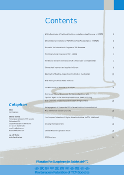
runtime in seconds (up to 3000)
SAT
103
102
101
FKA(HHM)
100
FKA(mf)
FKA(th)
FKB(HHM,rMin)
10−1
FKB(mf et al.)
reduction to SAT
20
24
28
32
reduction
36
number k of variables
Fig. 1. Runtimes and reduction ratio on M(k)
Matching M(k). The formula Mk of k variables (k even) consists of the terms
e k equivalent
{{xi , xi+1 } : 1 ≤ i < k, i is even}. Thus, |Mk | = k/2. The formula M
to Mk consists of the 2k/2 terms obtained by choosing one variable from every
e k ). Notice that the size of M(k)
term of Mk . The instance M(k) is the pair (Mk , M
is exponential in k. Simply said, the matching instances are pairs of equivalent
formulae, where one formula is exponentially larger than the other.
Figure 1 shows the runtimes for the matching instances. It shows that the
FKB-implementations are the slowest, the FKA-implementations are intermediate and the reduction to Sat is the fastest. For the reduction to Sat, the
reduction ratio shows how much of the runtime was used by the reduction function and by the Sat-solver. One can see that the new FKA-implementation is
better than the old one.
Threshold TH(k). The formula Tk of k variables is the set of terms {{xi , xj } :
e k equivalent to Tk
1 ≤ i < j ≤ k, j is even}. Thus, |Tk | = k 2 /4. The formula T
e
is Tk = {{1, . . . , 2t − 1} ∪ {2t + 2, 2t + 4, . . . , k} : 1 ≤ t ≤ k/2} ∪ {{2, 4, . . . , k}}.
e k | = k/2+1. The instance TH(k) is (Tk , T
e k ) and has size in O(k 2 ).
This yields |T
Simply said, the threshold instances are pairs of equivalent formulae, where one
formula is quadratic in the size of the other.
Figure 2 shows the runtimes for the threshold instances. It shows that the
old FKA-implementation is the slowest, and the old FKB-implementation and
the new FKB(rMin) are the fastest among the FK-implementations. The reason
is that the choice of the variable does not really matter on these instances, and
using a strategy wastes time. Again, the reduction to Sat is the fastest and
seems to have the slowest slope.
Self Dual Threshold SDTH(k). The formula STk of k variables (k even) is
e k−2 }.
the set of terms {{xk−1 , xk }}∪{{xk }∪m : m ∈ Tk−2 }∪{{xk−1 }∪m : m ∈ T
Note that STk read as DNF is equivalent to STk read as CNF. The instance
runtime in seconds (up to 100)
102
SAT
FKA(HHM)
101
FKA(mf),FKB(MOMs)
FKA(th)
FKB(HHM,rMin)
FKB(BOHM)
FKB(CRH)
100
reduction to SAT
10−1
reduction
200
400
600
800
1,000
number k of variables
Fig. 2. Runtimes and reduction ratio on TH(k)
runtime in seconds (up to 150)
SDTH(k) is (STk , STk ) and has size O(k 2 ). Simply said, the self dual threshold
instances are pairs of equivalent formulae of the same size.
Figure 3 shows the runtimes for the self-dual-threshold instances. It shows
that the old FKA-implementation is the slowest, but the new FKB(rMin)—that
was quite fast on the threshold instances—is very slow, too. The other new
FKB-implementations are the fastest among the FK-implementations. Again,
the reduction to Sat is the fastest.
SAT
102
101
FKA(HHM)
FKA(mf)
FKA(th)
100
FKB(HHM)
FKB(rMin)
FKB(BOHM)
FKB(MOMs)
FKB(CRH)
10−1
reduction to SAT
100
200
300
400
500
600
700
800
reduction
900 1,000
number k of variables
Fig. 3. Runtimes and reduction ratio on SDTH(k)
Connect-4 L(r) and W(r). “Connect-4” is a board game. Each row of the
dataset corresponds to a minimal winning (W) or losing (L) stage of the first
player, and is represented as a term. A term of an equivalent formula of a set
of winning stages (represented as a formula in DNF or CNF) is a minimal way
SAT
102
101
FKA(mf)
100
FKB(HHM)
FKB(rMin)
FKB(MOMs)
FKB(CRH)
10−1
W(1600)
W(800)
W(400)
W(200)
W(100)
L(800)
L(400)
L(200)
L(100)
reduction to SAT
L(1600)
runtime in seconds (up to 250)
to disturb winning/losing moves of the first player. To form a dataset, we take
the first r rows of the minimal winning stage (called Wr ) and the first r rows of
the minimal losing stage (called Lr ) [9,26]. To compute the equivalent formula
e r and W
f r we used the DL-algorithm [9]. Thus, we have L(r) = (Lr , L
e r ) and
L
f
W(r) = (Wr , Wr ) as instances. The set of testdata are from the UC Irvine
Machine Learning Repository [24]. It is used to compare algorithms that compute
equivalent normal forms. The smallest formula L(100) consists of 2,441 terms
with 77 variables, and L(1600) is the largest and has 214,361 terms with 81
variables. W(100) has a size of 387 terms with 76 variables, and W(3200) has
462,702 terms with 82 variables. Figure 4 shows the runtimes for the Connect-4
red.
L(k)
W(k)
Fig. 4. Runtimes and reduction ratio on L(r) and W(r)
instances. Only few instances were solvable within the given time bound. All FKimplementations behave similar, and for sake of clarity we left some of them out
in Figure 4. The new FKB(CRH) is the fastest among the FK-implementations.
As before, the reduction to Sat is the fastest.
BMS-WebView-2 BMS(s) and accidents AC(s). This testdata is generated by enumerating all maximal frequent sets from datasets “BMS-WebView-2”
and “accidents”. For a dataset and a support threshold s, an itemset is called
frequent if it is included in at least s members, and infrequent otherwise. A
frequent itemset included in no other frequent itemset is called a maximal frequent itemset, and an infrequent pattern including no other infrequent itemset
is called a minimal infrequent itemset. A minimal infrequent itemset is included
in no maximal frequent itemset, and any subset of it is included in at least
one maximal frequent itemset. Thus, the dual of the set of the complements of
maximal frequent itemsets is the set of minimal infrequent itemsets [26]. Note,
if we want to check the correctness of enumerating all maximal frequent sets
we can use Monet, because it is equivalent to this problem [2]. The problem
instances are generated by enumerating all maximal frequent sets from datasets
runtime in seconds (up to 700)
103
SAT
102
101
FKA(HHM)
FKA(mf)
10
0
FKA(th)
FKB(HHM)
FKB(rMin)
FKB(BOHM)
10−1
FKB(MOMs)
FKB(CRH)
red.
AC(k) BMS(k)
BMS(30)
BMS(50)
BMS(100)
BMS(400)
BMS(200)
BMS(500)
BMS(800)
AC(50k)
AC(70k)
AC(90k)
AC(110k)
AC(130k)
AC(150k)
AC(200k)
reduction to SAT
Fig. 5. Runtimes and reduction ratio on AC(s) and BMS(s)
BMS-WebView-2 BMS(s) and accidents AC(s) with threshold s, taken from
Frequent Itemset Mining Implementations Repository (FIMI) [25]. The smallest
formula AC(150k) has a size of 1,486 terms with 64 variables, and the largest is
AC(30k) with 320,657 terms and 442 variables. BMS(500) has a size of 17,143
terms with 3340 variables, and BMS(30) has 2,314,875 terms with 3340 variables. Figure 5 shows the runtimes for the AC and BMS instances. The BMS
instances show impressively, how good the reduction to Sat works.
The experiments described up to now used instances that consist of equivalent
formulae. To produce non-equivalent instances, we randomly delete variables
and terms in the above formulae. If we delete few variables or terms, we obtain
few conflict assignments. We compare some experiments on 236 non-equivalent
instances with thresholds of 60 and 360 seconds, where mf(¬UP) denotes the
mf-strategy without UP (see Table 1). The reduction to Sat solves all instances
within a time limit of 360 seconds, whereas our best implementation only solves
223 of 236 instances with this time. Furthermore, the experiments show that unit
propagation (UP) helps to solve more non-equivalence instances, since without
unit propagation less instances are solved. The runtimes do not depend on the
classes of test data introduced above.
seconds
60
360
FKA
FKB
reduction
mf(¬UP) mf HHM mf(¬UP) mf MOMs BOHM CRH HHM to Sat
194
209
201 166
223 196
162
201
181
213
182
216
148
186
143
188
161
189
221
236
Table 1. Non-equivalent instances (of 236) solved within 60 and 360 seconds
Finally, we show that in order to solve Monet using reduction to Sat with
a Sat-solver, it is much better to use the reduction function f (see Section 4)
than the usual Tseitin-translation [21]. Table 2 shows that using the Tseitintranslation the runtimes are worse than using the FK-algorithms.
reduction
using f
using Tseitin-translation
max. of FK-algorithms
22
M(k)
24
250
0.1
94
0.2
453
0.1
44
1.9
5.1
FKB(HHM)
8
TH(k)
500
700
0.2
854
0.3
3604
SDTH(k)
250
400
0.3
539
0.7
4974
136
563
20.5
FKA(HHM)3
211
Table 2. Comparison of runtimes of different reductions to Sat in seconds
6
Conclusion
The main finding is that a good reduction function and a Sat-solver provides
a more effective way for Monet than any current implementation of the FKalgorithms. It is a little surprising that it does not help to use the Tseitin translation only. Essentially, our reduction solves one direction of the equivalence test,
and the Sat-solver solves the other direction. Eventually, it is not that surprising
that the Sat-solvers are better than the implementations of the FK-algorithms.
On the other hand, we could improve the old implementations of the FKalgorithms [3] by using better data structures and unit propagation. Among
the strategies for finding a splitting variable, it seems that MOMs is a good
choice. This is not that surprising because MOMs is similar to choosing the
most frequent variable, and the latter is a straightforward strategy intended in
the formulation of FK-algorithm A [2].
Our next steps will be to figure out which strategies of Sat-solvers are responsible for the fast solution of reduced Monet instances and to see whether
they can be integrated into the FK-algorithms. For example, clause learning
seems to be useless for the FK-algorithms. Does the Sat-solver use it however
for solving Monet instances? Moreover, the clauses obtained from the reduction
function are easy in the sense that they are not needed for the NP-hardness of
Sat—otherwise Monet would be coNP-complete. Therefore, one can assume
that the “full power” of Sat-solvers is not necessary in order to solve reduced
Monet instances fast. Another question is whether it makes the equivalence test
easier if one checks both implication directions separately. The combination of
reduction and Sat-solver works this way, whereas the FK-algorithms recursively
make equivalence tests on decreasing formulae.
Acknowledgements The authors thank Sebastian Kuhs for some implementations, and Markus Chimani and Stephan Kottler for helpful comments.
References
1. Kavvadias, D.J., Stavropoulos, E.C.: Checking monotone Boolean duality with
limited nondeterminism. Technical Report TR2003/07/02, Univ. of Patras (2003)
2. Fredman, M.L., Khachiyan, L.: On the complexity of dualization of monotone
disjunctive normal forms. Journal of Algorithms 21(3) (1996) 618–628
3
Note that FKB(HHM) does not finish on SDTH(400).
3. Hagen, M., Horatschek, P., Mundhenk, M.: Experimental comparison of the two
Fredman-Khachiyan-algorithms. In: Proc. ALENEX. (2009) 154–161
4. Reith, S.: On the complexity of some equivalence problems for propositional calculi.
In: Proc. MFCS. (2003) 632–641
5. Eiter, T., Gottlob, G.: Hypergraph transversal computation and related problems
in logic and AI. In: Proc. JELIA 2002. Volume 2424 of LNCS. Springer (2002)
549–564
6. Eiter, T., Gottlob, G., Makino, K.: New results on monotone dualization and
generating hypergraph transversals. SIAM J. on Computing 32(2) (2003) 514–537
7. Papadimitriou, C.H.: NP-completeness: A retrospective. In: Proc. ICALP. (1997)
2–6
8. Bailey, J., Manoukian, T., Ramamohanarao, K.: A fast algorithm for computing
hypergraph transversals and its application in mining emerging patterns. In: Proc.
of the 3rd IEEE Intl. Conference on Data Mining (ICDM 2003). (2003) 485–488
9. Dong, G., Li, J.: Mining border descriptions of emerging patterns from dataset
pairs. Knowledge and Information Systems 8(2) (2005) 178–202
10. Khachiyan, L., Boros, E., Elbassioni, K.M., Gurvich, V.: An efficient implementation of a quasi-polynomial algorithm for generating hypergraph transversals. Discrete Applied Mathematics 154(16) (2006) 2350–2372
11. Kavvadias, D.J., Stavropoulos, E.C.: An efficient algorithm for the transversal
hypergraph generation. J. of Graph Algorithms and Applications 9(2) (2005) 239–
264
12. Lin, L., Jiang, Y.: The computation of hitting sets: Review and new algorithms.
Information Processing Letters 86(4) (2003) 177–184
13. Torvik, V.I., Triantaphyllou, E.: Minimizing the average query complexity of learning monotone Boolean functions. INFORMS Journal on Computing 14(2) (2002)
144–174
14. Uno, T., Satoh, K.: Detailed description of an algorithm for enumeration of maximal frequent sets with irredundant dualization. In: Proc. FIMI. (2003)
15. Davis, M., Logemann, G., Loveland, D.W.: A machine program for theoremproving. Commun. ACM 5 5(7) (1962) 394–397
16. Pretolani, D.: Efficiency and stability of hypergraph sat algorithms. In: Proc.
DIMACS Challenge II Workshop. (1993)
17. Buro, M., B¨
uning, H.K.: Report on a SAT competition (1992)
18. Kullmann, O.: Investigating the behaviour of a sat solver on random formulas.
Technical Report CSR 23-2002, University of Wales (2002)
19. Quine, W.: Two theorems about truth functions. Boletin de la Sociedad
Matem´
atica Mexicana 10 (1953) 64–70
20. Tamaki, H.: Space-efficient enumeration of minimal transversals of a hypergraph.
In: Proc. SIGAL. (2000) 29–36
21. Tseitin, G.S.: On the complexity of derivation in propositional calculus. In Slisenko,
A., ed.: Studies in constructive mathematics and mathematical logics, Part II.
(1968) 115–125
22. Galesi, N., Kullmann, O.: Polynomial time SAT decision, hypergraph transversals
and the hermitian rank. In: Proc. SAT 2004. (2004)
23. Le Berre, D., Parrain, A.: The Sat4j library, release 2.2. Journal on Satisfiability,
Boolean Modeling and Computation 7 (2010) 59–64
24. Repository, UCI: http://archive.ics.uci.edu/ml/ (2010)
25. Repository, FIMI: http://fimi.ua.ac.be/ (2010)
26. Murakami, K.: Personal communication (2010)