
How To Use iSubpathwayMiner Contents Chunquan Li July 8, 2012
How To Use iSubpathwayMiner
Chunquan Li
July 8, 2012
Contents
1 Overview
2
2 The methods of graph-based reconstruction of pathways
2.1 Convert KGML files of KEGG pathways to a list in R . . . . . . . . . . . . . . . . . . .
2.2 Convert metabolic pathways to graphs . . . . . . . . . . . . . . . . . . . . . . . . . . . .
2.2.1 The method to convert metabolic pathways to graphs . . . . . . . . . . . . . . .
2.2.2 Some simple examples of operating pathway graphs . . . . . . . . . . . . . . . .
2.3 Convert non-metabolic pathways to graphs . . . . . . . . . . . . . . . . . . . . . . . . .
2.3.1 The default method to convert non-metabolic pathways to graphs . . . . . . . .
2.3.2 The alternative method to convert non-metabolic pathways to graphs . . . . . .
2.4 Convert pathway graphs to other derivative graphs . . . . . . . . . . . . . . . . . . . . .
2.4.1 Convert pathway graphs to undirected graphs . . . . . . . . . . . . . . . . . . . .
2.4.2 Map current organism-specific gene identifiers to nodes in pathway graphs . . . .
2.4.3 Filter nodes of pathway graphs . . . . . . . . . . . . . . . . . . . . . . . . . . . .
2.4.4 Simplify pathway graphs as graphs with only gene products (or only compounds)
as nodes . . . . . . . . . . . . . . . . . . . . . . . . . . . . . . . . . . . . . . . . .
2.4.5 Expand nodes of pathway graphs . . . . . . . . . . . . . . . . . . . . . . . . . . .
2.4.6 Get simple pathway graphs . . . . . . . . . . . . . . . . . . . . . . . . . . . . . .
2.4.7 Merge nodes with the same names . . . . . . . . . . . . . . . . . . . . . . . . . .
2.5 The integrated application of pathway reconstruction methods . . . . . . . . . . . . . .
2.5.1 Example 1: enzyme-compound (KO-compound) pathway graphs . . . . . . . . .
2.5.2 Example 2: enzyme-enzyme (KO-KO) pathway graphs . . . . . . . . . . . . . . .
2.5.3 Example 3: compound-compound pathway graphs . . . . . . . . . . . . . . . . .
2.5.4 Example 4: organism-specific gene-gene pathway graphs . . . . . . . . . . . . . .
3 Topology-based analysis of pathways
3.1 The basic analyses for pathway graphs . . . . . . . . . . . . . . . . . . . . . . . . . . . .
3.1.1 Node methods: degree, betweenness, local clustering coefficient, etc. . . . . . . .
3.1.2 Edge method: shortest paths . . . . . . . . . . . . . . . . . . . . . . . . . . . . .
3.1.3 Graph method: degree distribution, diameter, global clustering coefficient, density, etc. . . . . . . . . . . . . . . . . . . . . . . . . . . . . . . . . . . . . . . . . .
3.2 Topology-based pathway analysis of molecule sets . . . . . . . . . . . . . . . . . . . . . .
3.2.1 Topology-based pathway analysis of gene sets . . . . . . . . . . . . . . . . . . . .
1
2
3
4
4
7
8
8
9
9
11
11
12
13
14
14
14
15
15
17
17
18
18
18
18
20
21
22
22
4 Annotation and identification of pathways
4.1 Annotate molecule sets and identify entire pathways . . . . . . . . . .
4.1.1 Annotate gene sets and identify entire pathways . . . . . . . .
4.1.2 Annotate compound sets and identify enire pathways . . . . .
4.1.3 Annotate gene and compound sets and identify entire pathways
4.1.4 Other examples . . . . . . . . . . . . . . . . . . . . . . . . . . .
4.2 The k-cliques method to identify subpathways based on gene sets . . .
4.3 The Subpathway-GM method to identify metabolic subpathways . . .
.
.
.
.
.
.
.
.
.
.
.
.
.
.
.
.
.
.
.
.
.
.
.
.
.
.
.
.
.
.
.
.
.
.
.
.
.
.
.
.
.
.
.
.
.
.
.
.
.
.
.
.
.
.
.
.
.
.
.
.
.
.
.
.
.
.
.
.
.
.
25
25
25
27
29
29
31
31
5 Visualize a pathway graph
5.1 Change node label of the pathway graph . . . . . . . . . . . . .
5.2 The basic commands to visualize a pathway graph with custom
5.3 The layout style of a pathway graph in R . . . . . . . . . . . .
5.4 Visualize the result graph of pathway analyses . . . . . . . . .
5.5 Export a pathway graph . . . . . . . . . . . . . . . . . . . . . .
.
.
.
.
.
.
.
.
.
.
.
.
.
.
.
.
.
.
.
.
.
.
.
.
.
.
.
.
.
.
.
.
.
.
.
.
.
.
.
.
.
.
.
.
.
.
.
.
.
.
35
35
37
38
39
43
6 Data management
6.1 Set or update the current organism and the type of gene identifier . . . . . . . . . . . .
6.2 Update pathway data . . . . . . . . . . . . . . . . . . . . . . . . . . . . . . . . . . . . .
6.3 Load and save the environment variable of the system . . . . . . . . . . . . . . . . . . .
43
43
44
44
7 Session Info
45
1
. . .
style
. . .
. . .
. . .
.
.
.
.
.
Overview
This vignette demonstrates how to easily use the iSubpathwayMiner package. This package can implement the graph-based reconstruction and analysis of the KEGG pathways. (1) Our system provides
many strategies of converting pathways to graph models (see the section 2). Ten functions related to
conversion from pathways to graphs are developed. Furthermore, the combinations of these functions
can get many combined conversion strategies of pathway graphs (> 20). The system can also support
topology-based pathway analysis of molecule sets (see the section 3.2). (2) The iSubpathwayMiner can
support the annotation and identification of entire pathways based on molecule (gene and/or metabolite) sets (see the section 4.1). (3) The iSubpathwayMiner provides the k-clique method for identification
of metabolic subpathways based on gene sets (see the section 4.2). (4) The iSubpathwayMiner provides
the Subpathway-GM method for identification of metabolic subpathways based on gene and metabolite
sets (see the section 4.3 new!).
2
The methods of graph-based reconstruction of pathways
The section introduces many strategies for converting pathways to different types of graphs. We
firstly need to use the function getPathway to convert KGML files (KEGG Markup Language, http:
//www.genome.jp/kegg/xml/) of KEGG pathways to a list variable in R, which is used to store pathway data in the iSubpathwayMiner system (see the section 2.1). We can then use the function getMetabolicGraph or getNonMetabolicGraph to convert metabolic pathways or non-metabolic pathways
to graphs (Figure 1 and 2). The function getMetabolicGraph constructs graphs based on reaction
information of KGML files of pathways (see the section 2.2). The function getNonMetabolicGraph
constructs graphs based on relation information (see the section 2.3). After using the function getMetabolicGraph or getNonMetabolicGraph to convert pathways to graphs, users can change these pathway
graphs to other derivative graphs. We develop the function getUGraph, mapNode, filterNode, simplifyGraph, mergeNode, getSimpleGraph, and expandNode (see the section 2.4). Through these functions,
2
many graph-based reconstruction strategies of pathways can be done such as constructing undirected
graphs, organism-specific and idType-specific graphs, the metabolic graphs with enzymes (compounds)
as nodes and compounds (enzymes) as edges, etc. Furthermore, the combination of these functions
can also get more useful pathway graphs (see the section 2.5). For example, we can construct the directed/undirected pathway graphs of enzyme-compound (see the section 2.5.1), enzyme-enzyme (see the
section 2.5.2), KO-KO (see the section 2.5.2), compound-compound (see the section 2.5.3), organismspecific gene-gene (see the section 2.5.4), etc. Most of these conversions represent current major applications [Smart et al., 2008, Schreiber et al., 2002, Klukas and Schreiber, 2007, Kanehisa et al., 2006,
Goffard and Weiller, 2007, Koyuturk et al., 2004, Hung et al., 2010, Xia and Wishart, 2010, Jeong et al., 2000,
Antonov et al., 2008, Guimera and Nunes Amaral, 2005, Draghici et al., 2007, Li et al., 2009, Ogata et al., 2000,
Hung et al., 2010, Barabasi and Oltvai, 2004]. The following sections will detailedly introduce the usage
of the functions relative to graph-based conversion of pathways.
2.1
Convert KGML files of KEGG pathways to a list in R
The KEGG Markup Language (KGML) is an exchange format of KEGG pathway data. In a KGML
file (.xml), the pathway element is a root element. The entry element stores information about nodes
of the pathway, including the attribute information (id, name, type, link, and reaction), the ”graphics”
subelement, the ”molecule” subelement. The relation element stores information about relationship
between gene products (or between gene products and compounds). It includes the attribute information
(entry1, entry2, and type), and the ”subtype” subelement that specifies more detailed information about
the interaction. The reaction element stores chemical reaction between a substrate and a product. It
includes the attribute information (id, name, and type), the ”substrate” subelement, and the ”product”
subelement. Detailed information is provided in http://www.genome.jp/kegg/xml/docs/.
In KEGG, there are two fundamental controlled vocabularies for matching genes to pathways. Enzyme commission (EC) numbers are traditionally used as an effective vocabulary for annotating genes
to metabolic pathways. With the rapid development of KEGG, more and more non-metabolic pathways
including genetic information processing, environmental information processing and cellular processes
have been added to KEGG PATHWAY database. KEGG Orthology (KO) identifiers, which overcome limitations of enzyme nomenclature and integrate the pathway and genome information, have
become a better controlled vocabulary for annotating genes to both metabolic and regulatory pathways [Kanehisa et al., 2006]. Therefore, KEGG has provided the KGML files of reference metabolic
pathways linked to EC identifiers, reference metabolic pathways linked to KO identifiers, and reference
non-metabolic pathways linked to KO identifiers. They can be obtained from KEGG ftp site.
The function getPathway can convert the above KGML files to a list variable in R, which is used as
pathway data in our system. The conversion only changes data structure in order to efficiently operate
data in R environment. After conversion, most of original information about pathways are not ignored
although data structure changed. The list that stores pathway information will be used as the input
of other functions such as getMetabolicGraph and getNonMetabolicGraph. The following commands can
convert KGML files of metabolic pathways to a list in R.
>
>
+
>
>
#get path of the KGML files
path<-paste(system.file(package="iSubpathwayMiner"),
"/localdata/kgml/metabolic/ec/",sep="")
#convert pathways to a list in R
p<-getPathway(path,c("ec00010.xml","ec00020.xml"))
3
2.2
2.2.1
Convert metabolic pathways to graphs
The method to convert metabolic pathways to graphs
The function getMetabolicGraph can convert metabolic pathways to graphs. A result graph mainly
contains three types of nodes: compounds, gene products (enzymes, KOs, or genes encoding them),
and maps that represent pathways linked with the current pathway. Edges are mainly constructed
from reactions. Specially, if a compound participates in a reaction as a substrate or product, a directed edge connects the compound node to the reaction node (enzymes, KOs, or genes). That is,
substrates of a reaction are connected to the reaction node (enzymes, KOs, or genes) and the reaction
node is connected to products. For substrates, they are directed toward the reaction node. For products, the reaction node is directed toward them. Reversible reactions have twice edges of irreversible
reactions. The conversion strategy of pathway graphs has the advantage that graph algorithms and
standard graph drawing techniques can be used. More importantly, almost all information can be efficiently stored in the kind of graph model. The similar strategy is also adopt by many study groups
[Smart et al., 2008, Klukas and Schreiber, 2007, Goffard and Weiller, 2007, Goffard and Weiller, 2007,
Koyuturk et al., 2004].
In addition, a compound and a linked map will be connected by an edge if they have relationships get
from relation element of the KGML file. Other information such as node attribute, pathway attribute
(e.g., pathway name), etc. are converted to attribute of graph.
The following commands can convert metabolic pathways to graphs.
>
>
+
>
>
>
>
#get path of the KGML files
path<-paste(system.file(package="iSubpathwayMiner"),
"/localdata/kgml/metabolic/ec/",sep="")
#convert pathways to a list in R
p<-getPathway(path,c("ec00010.xml"))
#convert metabolic pathways to graphs
gm<-getMetabolicGraph(p)
The following commands can visualize the graph of the Glycolysis / Gluconeogenesis pathway. Figure
1 shows the result graph. In the figure, the blue rectangle nodes represent enzymes. The circle nodes
represent compounds. The white rectangle nodes represent maps.
> #name of graph gm[[1]]
> gm[[1]]$title
[1] "Glycolysis / Gluconeogenesis"
> #visualize
> plotGraph(gm[[1]])
For a pathway graph, the function summary can print the number of nodes and edges, names of node
and edge attributes, etc. as follows:
> summary(gm[[1]])
IGRAPH DN-B 94 183 -- path:ec00010
attr: name (g/c), number (g/c), org (g/c), title (g/c), image (g/c),
link (g/c), name (v/c), id (v/c), names (v/c), type (v/c), reaction
(v/c), link (v/c), graphics_name (v/c), graphics_fgcolor (v/c),
graphics_bgcolor (v/c), graphics_type (v/c), graphics_x (v/c),
graphics_y (v/c), graphics_width (v/c), graphics_height (v/c),
graphics_coords (v/c)
4
TITLE:Glycolysis / Gluconeogenesis
Starch and sucrose metabolism
●
2.7.1.41
3.1.3.10
C00103
5.4.2.2
3.1.3.9
●
●
C00267
5.1.3.3
C00221
●
●
C06186 2.7.1.69
C01451 2.7.1.69
●
●
●
●
●
●
●
●
●
2.7.1.69 C00031
2.7.1.1 2.7.1.63
C00668
2.7.1.2 2.7.1.147
5.1.3.15 5.3.1.9
5.3.1.9
2.7.1.1 2.7.1.63
C01172
5.3.1.9
C05345
2.7.1.2 2.7.1.147
3.1.3.11 2.7.1.11 2.7.1.146
C06187 3.2.1.86
C05378
C06188 3.2.1.86
4.1.2.13
●
●
●
●
C00111
Pentose phosphate pathway
C00118
5.3.1.1
1.2.1.12 1.2.1.59
●
5.4.2.4 C00236
2.7.2.3
C01159
Carbon fixation in photosynthetic organisms
1.2.7.5 1.2.7.6
1.2.1.9
3.1.3.13 C00197
5.4.2.1
C00631
4.2.1.11
●
C00036
4.1.1.32
4.1.1.49
C00074
Pyruvate metabolism
1.2.7.1
Citrate cycle (TCA cycle)
●
●
2.7.1.40
C00068
6.2.1.1
C00024
●
2.3.1.12
C16255
6.2.1.13
C15973
●
1.8.1.4
●
C00033
●
1.2.4.1
C05125
●
4.1.1.1
C15972
1.2.1.3
1.2.1.5
●
C00084
1.2.4.1
4.1.1.1
●
C00022
1.1.1.27
Propanoate metabolism
1.1.1.1
1.1.2.7
1.1.2.8
1.1.1.2
●
C00469
Figure 1: The Glycolysis / Gluconeogenesis pathway graph.
5
●
C00186
The function str can display the information similar to the function summary. In addition, the
function also displays edges, graph attributes, node attributes, and edge attributes. The following
command prints all information of a pathway graph:
> str(gm[["00010"]],v=TRUE,e=TRUE,g=TRUE)
Because the pathway graph is usually too large, here we only display its subgraph with five nodes in
order to save page space.
> #display a subgraph with 5 nodes.
> sgm<-induced.subgraph(gm[[1]],V(gm[[1]])[1:5])
> str(sgm,g=TRUE,v=TRUE,e=TRUE)
IGRAPH DN-B 5 5 -- path:ec00010
+ attr: name (g/c), number (g/c), org (g/c), title (g/c), image (g/c),
link (g/c), name (v/c), id (v/c), names (v/c), type (v/c), reaction
(v/c), link (v/c), graphics_name (v/c), graphics_fgcolor (v/c),
graphics_bgcolor (v/c), graphics_type (v/c), graphics_x (v/c),
graphics_y (v/c), graphics_width (v/c), graphics_height (v/c),
graphics_coords (v/c)
+ graph attributes:
[[name]]
[1] "path:ec00010"
[[number]]
[1] "00010"
[[org]]
[1] "ec"
[[title]]
[1] "Glycolysis / Gluconeogenesis"
[[image]]
[1] "http://www.genome.jp/kegg/pathway/ec/ec00010.png"
[[link]]
[1] "http://www.genome.jp/kegg-bin/show_pathway?ec00010"
+ vertex attributes:
name id
names
type reaction
[1]
13 13 ec:4.1.2.13
enzyme rn:R01070
[2]
37 37 ec:1.2.1.3
enzyme rn:R00710
[3]
38 38 ec:6.2.1.13
enzyme rn:R00229
[4]
39 39 ec:1.2.1.5
enzyme rn:R00711
[5]
40 40 cpd:C00033 compound
unknow
link graphics_name
[1] http://www.kegg.jp/dbget-bin/www_bget?4.1.2.13
4.1.2.13
[2] http://www.kegg.jp/dbget-bin/www_bget?1.2.1.3
1.2.1.3
[3] http://www.kegg.jp/dbget-bin/www_bget?6.2.1.13
6.2.1.13
[4] http://www.kegg.jp/dbget-bin/www_bget?1.2.1.5
1.2.1.5
[5]
http://www.kegg.jp/dbget-bin/www_bget?C00033
C00033
graphics_fgcolor graphics_bgcolor graphics_type graphics_x graphics_y
[1]
#000000
#BFBFFF
rectangle
483
404
[2]
#000000
#BFBFFF
rectangle
289
943
[3]
#000000
#BFBFFF
rectangle
146
911
[4]
#000000
#BFBFFF
rectangle
289
964
[5]
#000000
#FFFFFF
circle
146
953
6
graphics_width graphics_height graphics_coords
[1]
46
17
unknow
[2]
46
17
unknow
[3]
46
17
unknow
[4]
46
17
unknow
[5]
8
8
unknow
+ edges (vertex names):
[1] 37->40 38->40 39->40 40->37 40->39
2.2.2
Some simple examples of operating pathway graphs
Since pathways can be converted to graphs, many analyses based on graph model are available by using
the functions provided in the igraph package. For example, we can get subgraph, degree, shortest path,
etc. Detailed information will be introduced in the section 3. Here, we only give some examples of
operating graphs, which are very important for effectively interpreting and operating pathway graphs.
We can get the name and number of one pathway, as follows:
> gm[[1]]$title
[1] "Glycolysis / Gluconeogenesis"
> gm[[1]]$number
[1] "00010"
We can get the attribute value of a node. In all attributes, the ”names” attribute is the most important.
It makes us able to identify the molecules the node includes. Its values are usually the identifiers of
compound, enzyme, gene, or KO, etc. The following commands can get ”names” attribute of the second
node:
> V(gm[[1]])[2]$names
[1] "ec:1.2.1.3"
The result shows that the second node is the enzyme identifier. We can also use another method to get
”names” attribute of the node
> get.vertex.attribute(gm[[1]],"names",2)
[1] "ec:1.2.1.3"
We can get other attributes. For example, the following command gets the ”type” attribute of the
second node:
> V(gm[[1]])[2]$type
[1] "enzyme"
The result shows that the second node is the enzyme.
An important application is to identify some nodes that meet the certain conditions. For example,
one is likely to want to find the enzyme ”ec:4.1.2.13” and ”ec:1.2.1.59” in pathway graph ”00010”, and
then calculate the shortest path between them in the graph. One may also want to identify the enzyme
”ec:4.1.2.3”, and then calculate its betweenness, which represents the importance of the node.
In order to do these, one firstly needs to get indexes of interesting nodes. Node indexes are used
as input of most of functions in igraph package. We then use functions in the igraph package (e.g.,
get.shortest.paths, betweenness, etc.) to get the analysis results. The following commands get indexes
of nodes with ”names”=”ec:4.1.2.13” and ”ec:1.2.1.59” in graph ”00010”, then calculate shortest path of
them.
7
>
>
>
>
>
>
>
#get indexes of nodes
index1<-V(gm[[1]])[V(gm[[1]])$names=="ec:4.1.2.13"]
index2<-V(gm[[1]])[V(gm[[1]])$names=="ec:1.2.1.59"]
#get shortest path
shortest.path<-get.shortest.paths(gm[[1]],index1,index2)
#display shortest path
shortest.path
[[1]]
[1] 1 89 81
> #convert indexes to names
> V(gm[[1]])[shortest.path[[1]]]$names
[1] "ec:4.1.2.13" "cpd:C00118"
"ec:1.2.1.59"
Calculate betweenness of the enzyme ”ec:4.1.2.3”.
> index1<-V(gm[[1]])[V(gm[[1]])$names=="ec:4.1.2.13"]
> betweenness(gm[[1]],index1)
13
1756.746
Note that we should see node index value using the function as.integer. The direct display is not
real node index value, but the value of the ”id” attribute of nodes.
> #node index value
> as.integer(index1)
[1] 1
> #direct display is not real node index value.
> index1
Vertex sequence:
[1] "13"
> #it is equal to the value of the "id" attribute.
> index1$id
[1] "13"
2.3
2.3.1
Convert non-metabolic pathways to graphs
The default method to convert non-metabolic pathways to graphs
The function getNonMetabolicGraph can convert non-metabolic pathways to directed graphs. An result
graph mainly contains two types of nodes: gene products (KOs) and maps that represent pathways
linked with the pathway graph. Sometimes, there are several compounds in pathways such as IP3,
DAG, cAMP, ca+, etc. Edges are obtained from relations. In particular, two nodes are connected by an
edge if they have relationships get from relation element of the KGML file. The relation element specifies
relationships between nodes. For example, the attribute PPrel represents protein-protein interaction
such as binding and modification. Other information such as node attribute, pathway attribute, etc.
is converted to attribute of graphs. The following commands can convert non-metabolic pathways to
graphs. The result graph of the MAPK signaling pathway is shown in Figure 2.
8
>
>
+
>
>
>
>
>
#get path
pathn<-paste(system.file(package="iSubpathwayMiner"),
"/localdata/kgml/non-metabolic/ko/",sep="")
pn<-getPathway(pathn,c("ko04010.xml","ko04020.xml"))
#Convert pathways to graphs
gn1<-getNonMetabolicGraph(pn)
#name of the first pathway
gn1[[1]]$title
[1] "MAPK signaling pathway"
> #visualize
> plotGraph(gn1[[1]])
2.3.2
The alternative method to convert non-metabolic pathways to graphs
In non-metabolic pathways, there are usually many different types of edges between nodes. There
are four fundamental types of edges including ECrel (enzyme-enzyme relation), PPrel (protein-protein
interaction), GErel (gene expression interaction) and PCrel (protein-compound interaction). Each fundamental type usually contains many subtypes such as compound, hidden compound, activation, inhibition, expression, repression, indirect effect, state change, binding/assoction, dissociation, and missing
interaction. Detailed information is provided in http://www.genome.jp/kegg/xml/docs/.
According to these substypes, we can obtain edge direction. For example, ”activation” means that
protein A activates B (A–>B). However, not all types of edges have definite direction. For example,
”binding/association” means that there is the binding or association relation between protein A and
protein B but we don’t know A–>B or B–>A. In addition, an edge is also likely to have no subtype and
thus we can’t know its direction. The argument ambiguousEdgeDirection can define direction of ambiguous edges according to subtype of edges. Users firstly define which subtype of edges are considered
as ambiguous edges by setting the argument ambiguousEdgeList. The default ambiguous edges include
”compound”, ”hidden compound”, ”state change”, ”binding/association”, ”dissociation”, and ”unknow”.
Then users can define their direction through setting the value of the argument ambiguousEdgeDirection
as one of ”single”, ”bi-directed” or ”delete”, which means to convert ambiguous edges to ”–>”, ”<–>”,
or to delete these ambiguous edges. The default value is ”bi-directed”.
The following commands convert pathways to graphs with ambiguous edges deleted. Compared with
Figure 2, some edges are deleted such as edges related with the compound ”C00076” because the default
ambiguous edges include ”compound”.
> #Convert pathways to graphs with ambiguous edges as deleted
> gn2<-getNonMetabolicGraph(pn,ambiguousEdgeDirection="delete")
2.4
Convert pathway graphs to other derivative graphs
After using the function getMetabolicGraph or getNonMetabolicGraph to convert pathways to graphs,
users can change these pathway graphs to other derivative graphs. The following section will detailedly
introduce the usage of the related functions.
We firstly construct metabolic pathway graphs (gm) and non-metabolic pathway graphs (gn) as
examples of input data. The commands are as follows:
>
>
>
+
##get metabolic pathway graphs
#get path of KGML files
path<-paste(system.file(package="iSubpathwayMiner"),
"/localdata/kgml/metabolic/ec/",sep="")
9
TITLE:MAPK signaling pathway
Phosphatidylinositol signaling system
●●●
K04466 ..>
C00575
K02580...
C01245 C00165
K04467... ..>
−−>
−−>
K04345
K04380
K04344... C00076
−−>
K04381
+p
−−>
K01047
K04353...
+p
K02582
K08018
+p
−−>
+p
K04349...
+p
−−>
K04355
K03176...
+p
+p
−−>
+p
K04350... K02677 −−>
K04372
+p +p
K04356...
−−−
K04374
+p
+p
−−>+p
−−>
−−−
−−−
K04373
K04370
K04365
−−>
−−>
−−−
K04361
K04357
−−−
+p
−−−−−− +p +p K04375
−−>
−−−
−−−
K04368
−−−
−−−
+p
+p
−e−>
−−−
−−−
−−−
−−−
−−|
−e−>
−−>
−−>
−−> K04366 +p
K03099
K04379
K02833...
K04378
K04362...
K04364
K04358
+pK04371
−−−
−−−
−e−>
+p K04376
−−−
−−−
+pK04369
−−>
+p−−|−−|
+p
−−>
K04359
K04363...
−−| −−|
−p
−p
K04367
+p
K04377
K08052
+p
+p
−−>
K04459
K04346...
K08053 K04352
K04458
+p
+p
K04348...
●
−−>
K03156
K03158
−−>
K04383...
K04386...
−−>
K04389
K04390
−−>
K04388...
K13375...
●
−−>
K04391
C00338
−−>
−−>
−−>
−−>
−−>
..>
..>
K04437
K04436
K03283
−−−
−−−
−−−
−−−−−−K04462
K04439
K04438
K04406 K04415−−−
−−−
−−−
−−−
+p
−−−
−−−
−−−
−−−
−−−
−−−
−−− −−− −−−
−−|
+pK04416 +p
K04407
K04430+p −−|
+p K04448
−−−
−−>
−−−
+p K04449
+pK04440
+pK04431
K04408
−−− −−−
−−−
−−−
−−−
−−>+pK04419
−−|
−p
+p
K04434...
−−|
+p
−−|
−p
−−>
+p
−−| −p −−| −p
+p
−−>
K04392...
K−−>
04409...
K04420...+p
+p
+p
K04450
K04422 K04457 K04459
K04375
p53 signaling pathway
K02187−−>
K04411... K04423
K04456 K04458
K04451
+p +p
+p
K04424
−−| −p
K03173−−>
K04414
−−|−p−p
−−| +p −−| −p −−|
K04376
K04425
+p
+p
−−>
+pK04432+p
+p K04452
+p
..>
−−> K04426
K02308
K04441
..>
+p
+p
−−| −p +p
+p
K04453
+pK04433
+p +p
K04403 +p
..>
K04454
+pK04427
+p
−−| −p K04460
K04404
K04442
−−−
−−−
+p
+p
K03175
K04455
−−−
K04461
+p
−−−
+p
K04443...
K04405
+p
+p
+p
−−> K04428
K04402
K04445
K04374
K05866
K04429
K04468
K04463+pK04464
Cell cycle
Apoptosis
Wnt signaling pathway
+p K04465
Figure 2: The MAPK signaling pathway graph with ambiguous edges as bi-directed.
10
>
>
>
>
#convert metabolic pathways to graphs
gm<-getMetabolicGraph(getPathway(path,c("ec00010.xml")))
#show title of pathway graphs
sapply(gm,function(x) x$title)
00010
"Glycolysis / Gluconeogenesis"
>
>
>
+
>
>
+
>
>
##get non-metabolic pathway graphs
#get path
path1<-paste(system.file(package="iSubpathwayMiner"),
"/localdata/kgml/non-metabolic/ko/",sep="")
#convert non-metabolic pathways to graphs
gn<-getNonMetabolicGraph(getPathway(path1,c("ko04010.xml")),
ambiguousEdgeDirection="bi-directed")
#show title of pathway graphs
sapply(gn,function(x) x$title)
04010
"MAPK signaling pathway"
Note that the variable gm is a list of metabolic pathway graphs. The variable gn is a list of non-metabolic
pathway graphs.
2.4.1
Convert pathway graphs to undirected graphs
The function getUGraph can convert directed graphs to undirected graphs. The following commands can
get the undirected simple pathway graph.
> #get undirected pathway graphs
> g1<-getUGraph(gm,simpleGraph=TRUE)
2.4.2
Map current organism-specific gene identifiers to nodes in pathway graphs
The function mapNode can map current organism-specific gene identifiers to nodes of graphs. We can
use the function getOrgAndIdType to know the type of organism and identifier in the current study:
> getOrgAndIdType()
[1] "hsa"
"ncbi-geneid"
The result means that the type of organism and identifier in the current study are Homo sapiens (hsa)
and Entrez gene identifiers (NCBI-geneid), which is the default value of the system (see the section 6).
The following commands use the function mapNode to map human gene identifiers (NCBI-geneid) to
nodes in pathway graphs. We can see the value of names attribute of some nodes revised.
> #see the names attribute of nodes.
> V(gm[[1]])[1:10]$names
[1] "ec:4.1.2.13" "ec:1.2.1.3"
"ec:6.2.1.13"
[6] "path:ec00030" "path:ec00500" "ec:4.1.1.1"
11
"ec:1.2.1.5"
"ec:1.1.1.2"
"cpd:C00033"
"ec:1.1.1.1"
>
>
>
>
>
#get the organism-specific and idType-specific graph
g1<-mapNode(gm)
#see the names attribute of nodes in the new graph.
#some node names are revised as NCBI-gene IDs
V(g1[[1]])[1:10]$names
[1]
[3]
[5]
[7]
[9]
"226 229 230"
"ec:6.2.1.13"
"cpd:C00033"
"path:ec00500"
"10327"
2.4.3
"217 219 223 224 501"
"218 220 221 222"
"path:ec00030"
"ec:4.1.1.1"
"124 125 126 127 128 130 131"
Filter nodes of pathway graphs
The function filterNode is used to filter ”not interesting” nodes. For example, it may be necessary to
ignore nodes with type=”map” when focusing on molecules such as compounds and gene products. The
function will delete nodes according to the argument nodeType and thus related edges are also deleted.
The following commands can delete nodes whose types are ”map”.
> #We display them before nodes are filtered
> V(gn[[1]])$type
[1]
[7]
[13]
[19]
[25]
[31]
[37]
[43]
[49]
[55]
[61]
[67]
[73]
[79]
[85]
[91]
[97]
[103]
[109]
[115]
[121]
[127]
[133]
>
>
>
>
"compound"
"compound"
"ortholog"
"ortholog"
"ortholog"
"ortholog"
"ortholog"
"ortholog"
"map"
"ortholog"
"ortholog"
"ortholog"
"ortholog"
"ortholog"
"ortholog"
"ortholog"
"ortholog"
"ortholog"
"ortholog"
"ortholog"
"ortholog"
"ortholog"
"ortholog"
"ortholog"
"compound"
"ortholog"
"ortholog"
"ortholog"
"ortholog"
"ortholog"
"ortholog"
"map"
"ortholog"
"ortholog"
"ortholog"
"ortholog"
"ortholog"
"ortholog"
"ortholog"
"ortholog"
"ortholog"
"ortholog"
"ortholog"
"ortholog"
"ortholog"
"ortholog"
"compound"
"ortholog"
"ortholog"
"ortholog"
"ortholog"
"ortholog"
"ortholog"
"map"
"ortholog"
"ortholog"
"ortholog"
"ortholog"
"ortholog"
"ortholog"
"ortholog"
"ortholog"
"ortholog"
"ortholog"
"ortholog"
"ortholog"
"ortholog"
"ortholog"
"compound"
"ortholog"
"ortholog"
"ortholog"
"ortholog"
"ortholog"
"ortholog"
"map"
"ortholog"
"ortholog"
"ortholog"
"ortholog"
"ortholog"
"ortholog"
"ortholog"
"ortholog"
"ortholog"
"ortholog"
"ortholog"
"ortholog"
"ortholog"
"ortholog"
"ortholog"
"ortholog"
"ortholog"
"ortholog"
"ortholog"
"ortholog"
"ortholog"
"map"
"ortholog"
"ortholog"
"ortholog"
"ortholog"
"ortholog"
"ortholog"
"ortholog"
"ortholog"
"ortholog"
"ortholog"
"ortholog"
"ortholog"
"ortholog"
"ortholog"
"ortholog"
"ortholog"
"ortholog"
"ortholog"
"ortholog"
"ortholog"
"map"
"ortholog"
"ortholog"
"ortholog"
"ortholog"
"ortholog"
"ortholog"
"ortholog"
"ortholog"
"ortholog"
"ortholog"
"ortholog"
"ortholog"
"ortholog"
"ortholog"
#delete nodes with type="map"
g1<-filterNode(gn,nodeType=c("map"))
#The "map" nodes are deleted in the new graph.
V(g1[[1]])$type
[1] "compound" "ortholog" "ortholog" "ortholog" "ortholog" "ortholog"
[7] "compound" "compound" "compound" "compound" "ortholog" "ortholog"
12
[13]
[19]
[25]
[31]
[37]
[43]
[49]
[55]
[61]
[67]
[73]
[79]
[85]
[91]
[97]
[103]
[109]
[115]
[121]
[127]
2.4.4
"ortholog"
"ortholog"
"ortholog"
"ortholog"
"ortholog"
"ortholog"
"ortholog"
"ortholog"
"ortholog"
"ortholog"
"ortholog"
"ortholog"
"ortholog"
"ortholog"
"ortholog"
"ortholog"
"ortholog"
"ortholog"
"ortholog"
"ortholog"
"ortholog"
"ortholog"
"ortholog"
"ortholog"
"ortholog"
"ortholog"
"ortholog"
"ortholog"
"ortholog"
"ortholog"
"ortholog"
"ortholog"
"ortholog"
"ortholog"
"ortholog"
"ortholog"
"ortholog"
"ortholog"
"ortholog"
"ortholog"
"ortholog"
"ortholog"
"ortholog"
"ortholog"
"ortholog"
"ortholog"
"ortholog"
"ortholog"
"ortholog"
"ortholog"
"ortholog"
"ortholog"
"ortholog"
"ortholog"
"ortholog"
"ortholog"
"ortholog"
"ortholog"
"ortholog"
"ortholog"
"ortholog"
"ortholog"
"ortholog"
"ortholog"
"ortholog"
"ortholog"
"ortholog"
"ortholog"
"ortholog"
"ortholog"
"ortholog"
"ortholog"
"ortholog"
"ortholog"
"ortholog"
"ortholog"
"ortholog"
"ortholog"
"ortholog"
"ortholog"
"ortholog"
"ortholog"
"ortholog"
"ortholog"
"ortholog"
"ortholog"
"ortholog"
"ortholog"
"ortholog"
"ortholog"
"ortholog"
"ortholog"
"ortholog"
"ortholog"
"ortholog"
"ortholog"
"ortholog"
"ortholog"
"ortholog"
"ortholog"
"ortholog"
"ortholog"
"ortholog"
"ortholog"
"ortholog"
"ortholog"
"ortholog"
"ortholog"
"ortholog"
"ortholog"
"ortholog"
"ortholog"
"ortholog"
"ortholog"
"ortholog"
Simplify pathway graphs as graphs with only gene products (or only compounds)
as nodes
When we focus on gene products, compounds may be not important. Similarly, gene products may
be not important when focusing on metabolites (compounds). For metabolic pathway graphs, a useful
approach is to get graphs with gene products (or compounds) as nodes and compounds (gene products)
as edges.
The function simplifyGraph can convert pathways to graphs with gene products (or compounds)
as nodes and compounds (or gene products) as edges. We take an example of constructing metabolic
pathway graphs with enzymes as nodes and compounds as edges. Firstly, all enzymes in a pathway
graph are used as nodes. For undirected, two nodes are then connected by an edge if their corresponding
reactions have a common compound. For directed, two nodes are connected by an edge if their corresponding reactions have a common compound and two nodes are reachable through the compound.
Finally, compound information is added into edge attribute of new graphs. Similarly, a metabolic pathway graph can be converted to a graph with compounds as nodes. Two nodes are connected by an edge
if they belong to the same reaction. Enzyme information is added into edge attribute of new graphs.
The following commands construct pathway graphs with enzymes as nodes and compounds as edges.
>
>
>
>
#get graphs with enzymes as nodes and compounds as edges
g1<-simplifyGraph(gm,nodeType="geneProduct")
#see the names attribute of three edges
E(g1[[1]])[1:3]$names
[1] "cpd:C00111;cpd:C00118" "cpd:C05378"
"cpd:C00118"
The following commands construct graphs with compounds as nodes and enzymes as edges.
>
>
>
>
#get graphs with compounds as nodes and enzymes as edges
g2<-simplifyGraph(gm,nodeType="compound")
#see the names attribute of three edges
E(g2[[1]])[1:3]$names
[1] "ec:1.2.1.3;ec:1.2.1.5" "ec:6.2.1.1"
"ec:2.7.1.69"
13
2.4.5
Expand nodes of pathway graphs
In pathways, some nodes may have multiple molecules, which are considered as molecules of ”paralogues”. For example, node PDE, which is the enzyme node in Purine metabolism (ec00230), maps
to two enzymes: PDE (ec:3.1.4.17) and cGMP-PDE (ec:3.1.4.35). The function expandNode is just used
to expand those nodes with multiple molecules. Users can select which types of nodes are expanded
using the argument nodeType. The default values represent that all nodes are expanded. The following
commands expand nodes of non-metabolic pathway graphs:
> #We firstly display node number before nodes are expanded
> vcount(gn[[1]])
[1] 133
>
>
>
>
>
##expand nodes in Graphs
g1<-expandNode(gn)
#We can see change of node number in the new graph:
#node number after nodes are expanded
vcount(g1[[1]])
[1] 197
The argument nodeType can determine which types of nodes should be expanded. Expanding nodes
with certain node types is also available. The following commands only expand nodes that belong to
gene products.
> #only expand nodes with type="enzyme" or "ortholog" in graphs
> g2<-expandNode(gn,nodeType=c("ortholog","enzyme"))
2.4.6
Get simple pathway graphs
If a graph is simple, it does not contain loop or/and multiple edges. A loop edge is an edge where the
two endpoints have the same node (vertex). Two edges are multiple edges if they have exactly the same
two endpoints. If graphs are not simple, some graph-based algorithms may be not applied. We can use
the function getSimpleGraph to get a simple graph. Note that information of multiple edges is kept in
edge attribute using ”;” as separator.
The function is.simple can check whether a graph is simple as follows:
> all(sapply(gm,is.simple))
[1] TRUE
2.4.7
Merge nodes with the same names
A pathway usually includes some nodes with the same names. For example, an enzyme may appear
repeatedly in a pathway. As shown in Figure 1, the Glycolysis / Gluconeogenesis pathway contain
enzymes that appear repeatedly such as 2.7.1.69, 4.1.1.1, etc. The function mergeNode can merge those
nodes with the same names. Therefore, each node in the result graph will has unique name. The edges
of the merged nodes are obtained from edges of original nodes. After nodes are merged, multiple edges
or loops may appear. The argument simpleGraph can delete them, which will return simple graphs (see
the section 2.4.6). The following commands can get the graph in which nodes with the same names are
merged.
> #get node number before merge
> vcount(gm[[1]])
14
[1] 94
>
>
>
>
#merge nodes
g1<-mergeNode(gm,simple=FALSE)
#get node number after merge
vcount(g1[[1]])
[1] 83
2.5
The integrated application of pathway reconstruction methods
In the section, we have provided some examples for converting pathways to graphs using the combination
of graph conversion functions. Through the combination of these functions, many conversion strategies
of pathway graphs can be implemented.
The section introduces some examples of pathway graphs. They include enzyme-compound (KOcompound) pathway graphs, enzyme-enzyme (KO-KO) pathway graphs, compound-compound pathway graphs, organism-specific gene-gene pathway graphs, etc. More detailed information is provided
in help of the package. These examples represent current major applications [Smart et al., 2008,
Schreiber et al., 2002, Klukas and Schreiber, 2007, Kanehisa et al., 2006, Goffard and Weiller, 2007, Koyuturk et al., 2004,
Hung et al., 2010, Xia and Wishart, 2010, Jeong et al., 2000, Antonov et al., 2008, Guimera and Nunes Amaral, 2005,
Draghici et al., 2007, Li et al., 2009, Ogata et al., 2000, Hung et al., 2010, Barabasi and Oltvai, 2004].
2.5.1
Example 1: enzyme-compound (KO-compound) pathway graphs
For metabolic pathways, the following commands can get pathway graphs with enzymes and compounds
as nodes.
>
>
>
>
#get graphs with enzymes and compounds as nodes
g1<-filterNode(gm,nodeType=c("map"))
#visualize
plotGraph(g1[[1]])
Figure 3 shows the result graph of the Glycolysis / Gluconeogenesis pathway. Compared with original
pathway graph (Figure 1), the ”map” nodes disappear in the new graph.
If we apply the above method to all metabolic pathways, we can get all metabolic pathway graphs
with enzymes and compounds as nodes. To do it easily, we have developed the function getMetabolicECCOGraph. The following command can use the function to get all metabolic pathway graphs with
enzymes and compounds as nodes.
> #get all metabolic pathway graphs with enzymes and compounds as nodes
> graphList<-getMetabolicECCOGraph()
The result of the function are equal to the result of the following commands:
> #get all metabolic pathway data
> metabolicEC<-get("metabolicEC",envir=k2ri)
> graphList<-filterNode(getMetabolicGraph(metabolicEC),nodeType=c("map"))
The variable metabolicEC stores all metabolic pathway data (see the section 6). The variable graphList
stores all metabolic pathway graphs with enzymes and compounds as nodes.
The following commands can get the corresponding undirected graphs, that is, the undirected graphs
with enzymes and compounds as nodes. The function getMetabolicECCOUGraph can get all results.
> #get the undirected graphs with enzymes and compounds as nodes
> g2<-filterNode(getUGraph(gm),nodeType=c("map"))
15
●
2.7.1.41
3.1.3.10
C00103
5.4.2.2
3.1.3.9
●
C00267
2.7.1.1
2.7.1.2
2.7.1.63
2.7.1.147
5.1.3.15
5.1.3.3
●
C00221
●
●
2.7.1.1
2.7.1.2
●
5.3.1.9
C01172
5.3.1.9
●
5.3.1.9
C05345
3.1.3.11
C06186
2.7.1.69
C06187
3.2.1.86
C01451
2.7.1.69
C06188
3.2.1.86
●
C00031
C00668
●
2.7.1.63
2.7.1.147
●
●
2.7.1.69
2.7.1.11
2.7.1.146
●
C05378
4.1.2.13
●
C00111
●
C00118
5.3.1.1
1.2.1.12
5.4.2.4
●
1.2.1.59
●
C00236
2.7.2.3
C01159
3.1.3.13
1.2.7.6
1.2.7.5
1.2.1.9
●
C00197
5.4.2.1
●
C00631
4.2.1.11
●
C00036
●
4.1.1.32
4.1.1.49
C00074
2.7.1.40
1.2.7.1
●
●
C00068
6.2.1.1
C00024
●
2.3.1.12
6.2.1.13
C15973
●
C00033
●
●
C16255
1.8.1.4
1.2.4.1
C05125
●
4.1.1.1
C15972
1.2.1.3
1.2.1.5
●
C00084
1.2.4.1
4.1.1.1
1.1.1.1
1.1.2.7
1.1.2.8
●
C00022
1.1.1.2
1.1.1.27
●
C00186
●
C00469
Figure 3: The Glycolysis / Gluconeogenesis pathway graph with enzymes and compounds as nodes.
Compared with original pathway graph (Figure 1), the ”map” nodes disappear in the new graph.
16
The following commands can get graphs with enzymes and compounds as nodes, in which each node
only contains one enzyme/compound and each enzyme/compound only appears once. The function
getMetabolicECCOEMGraph can get all results.
>
>
>
>
#get graphs with enzymes and compounds as nodes
#And, each node only contains one enzyme/compound and
#each enzyme/compound only appears once in the graph.
g3<-mergeNode(expandNode(filterNode(gm,nodeType=c("map"))))
The following commands can get the corresponding undirected graphs. The function getMetabol-
icECCOUEMGraph can get all results.
>
>
>
>
#get the undirected graphs with enzymes and compounds as nodes
#And, each node only contains one enzyme/compound and
#each enzyme/compound only appears once in the graph.
g4<-mergeNode(expandNode(filterNode(getUGraph(gm),nodeType=c("map"))))
2.5.2
Example 2: enzyme-enzyme (KO-KO) pathway graphs
For metabolic pathways, the following commands can get graphs with enzymes as nodes and compounds
as edges. The function getMetabolicECECGraph can get the results of all metabolic pathway graphs with
enzymes as nodes and compounds as edges.
> #get graphs with enzymes as nodes and compounds as edges
> g1<-simplifyGraph(filterNode(gm,nodeType=c("map")),nodeType="geneProduct")
The following commands can get the corresponding undirected graphs. The function getMetabolicECECUGraph can get all results.
> #get undirected graphs with enzymes as nodes and compounds as edges.
> g2<-simplifyGraph(filterNode(getUGraph(gm),nodeType=c("map")),nodeType="geneProduct")
The following commands can get graphs with enzymes as nodes and compounds as edges. And,
each node contains only one enzyme and each enzyme only appears once in the graph. The function
getMetabolicECECEMGraph can get all results.
>
>
>
+
#get graphs with enzymes as nodes and compounds as edges
#And, each node contains only one enzyme and each enzyme only appears once.
g3<-mergeNode(expandNode(simplifyGraph(filterNode(gm,
nodeType=c("map")),nodeType="geneProduct")))
The following commands can get the corresponding undirected graphs. The function getMetabol-
icECECUEMGraph can get all results.
>
>
>
+
#get undirected graphs with enzymes as nodes and compounds as edges.
#And, each node contains only one enzyme and each enzyme only appears once.
g4<-mergeNode(expandNode(simplifyGraph(filterNode(getUGraph(gm),
nodeType=c("map")),nodeType="geneProduct")))
2.5.3
Example 3: compound-compound pathway graphs
For metabolic pathways, the following commands can get graphs with compounds as nodes and enzymes
as edges. The function getMetabolicCOCOGraph with setting the argument type as ”EC” can get all
metabolic pathway graphs with compounds as nodes and enzymes as edges.
> #The graph with compounds as nodes and enzymes as edges
> g1<-simplifyGraph(filterNode(gm,nodeType=c("map")),nodeType="compound")
17
2.5.4
Example 4: organism-specific gene-gene pathway graphs
For metabolic pathways, the following commands can get graphs with organism-specific genes as nodes
and compounds as edges. And, each node contains only a gene and each gene only appears once in
the graph. The function getMetabolicGEGEEMGraph with setting the argument type as ”EC” can get all
metabolic pathway graphs with organism-specific genes as nodes and compounds as edges.
> #get graphs with organism-specific genes as nodes and compounds as edges
> g1<-mergeNode(expandNode(simplifyGraph(filterNode(mapNode(gm),
+ nodeType=c("map","enzyme")),nodeType="geneProduct")))
For non-metabolic pathways, the following commands can get graphs with organism-specific genes as
nodes and compounds as edges. Moreover, each node contains only a gene and each gene only appears
once in the graph. The function getNonMetabolicGEGEEMGraph can get all results.
> #get graphs with organism-specific genes as nodes
> g3<-mergeNode(expandNode(simplifyGraph(filterNode(mapNode(gn),
+ nodeType=c("map","ortholog")),nodeType="geneProduct")))
3
Topology-based analysis of pathways
3.1
The basic analyses for pathway graphs
Since pathways are able to be converted to different types of graphs, many analyses based on graph model
are available by using the functions provided in the igraph package. For example, we can get subgraph,
degree, shortest path, etc [Csardi and Nepusz, 2006]. Here, we will give some detailed examples of
operating graphs, nodes, edges, attributes. To do these, we firstly construct pathway graphs as the
example graphs of the basic analyses based on graph model. The commands are as follows:
We can get metabolic pathway graphs as follows:
>
>
+
>
>
>
>
#get path of KGML files
path<-paste(system.file(package="iSubpathwayMiner"),
"/localdata/kgml/metabolic/ec/",sep="")
#convert metabolic pathways to graphs with "map" node deleted
gmf<-filterNode(getMetabolicGraph(getPathway(path,c("ec00010.xml"))))
#show title of pathway graphs
sapply(gmf,function(x) x$title)
00010
"Glycolysis / Gluconeogenesis"
> #convert metablic pathways to graphs with enzymes as nodes and compounds as edges
> gmfs<-simplifyGraph(gmf,nodeType="geneProduct")
Figure 4 displays gmfs[[1]]. It is the Glycolysis / Gluconeogenesis pathway graph with enzymes as
nodes and compounds as edges. The ”map” nodes are deleted.
3.1.1
Node methods: degree, betweenness, local clustering coefficient, etc.
Degree (or connectivity) of a node is defined as the number of its adjacent edges [Csardi and Nepusz, 2006,
Barabasi and Oltvai, 2004, Huber et al., 2007]. It is a local quantitative measure of a node relative to
other nodes. The following commands can get the degree of the first node in the graph.
18
2.7.1.41
3.1.3.10
5.4.2.2
3.1.3.9
2.7.1.1
2.7.1.2
2.7.1.63
2.7.1.147
5.1.3.15
2.7.1.1
2.7.1.2
2.7.1.63
2.7.1.147
5.1.3.3
2.7.1.69
5.3.1.9
5.3.1.9
5.3.1.9
3.1.3.11
2.7.1.69
3.2.1.86
2.7.1.69
3.2.1.86
2.7.1.11
2.7.1.146
4.1.2.13
5.3.1.1
1.2.1.12
1.2.1.59
5.4.2.4
2.7.2.3
1.2.7.6
1.2.7.5
1.2.1.9
3.1.3.13
5.4.2.1
4.2.1.11
4.1.1.32
4.1.1.49
2.7.1.40
1.2.7.1
2.3.1.12
6.2.1.1
6.2.1.13
1.2.4.1
4.1.1.1
1.2.4.1
1.8.1.4
1.1.1.27
4.1.1.1
1.1.1.1
1.1.2.7
1.1.2.8
1.2.1.3
1.2.1.5
1.1.1.2
Figure 4: The Glycolysis / Gluconeogenesis pathway graph with enzymes as nodes and compounds as
edges. The ”map” nodes are deleted. The graph is stored in the variable gmfs[[1]].
19
> #get degree of nodes
> igraph::degree(gmfs[[1]],1)
13
12
We can see names of the first node as follows:
> #see name of the first node
> V(gmfs[[1]])[1]$names
[1] "ec:4.1.2.13"
The first node is the enzyme ”ec:4.1.2.13” and is at the right-top part of Figure 4.
We can identify enzyme ”ec:4.1.2.13” and get degree of a node with given names as follows:
>
>
>
>
#get indexes of nodes
index1<-V(gmfs[[1]])[V(gmfs[[1]])$names=="ec:4.1.2.13"]
#get degree of node
igraph::degree(gmfs[[1]],index1)
13
12
We may also want to calculate its betweeness, which is (roughly) defined by the number of shortest
paths going through a node [Csardi and Nepusz, 2006, Barabasi and Oltvai, 2004, Huber et al., 2007].
> #Calculate betweenness of enzyme "ec:4.1.2.13".
> betweenness(gmfs[[1]],index1)
13
960
The local clustering coefficient measures the probability that the adjacent nodes of a node are
connected.
> #Calculate the clustering coefficient of enzyme "ec:4.1.2.13".
> igraph::transitivity(gmfs[[1]],type="local",vids=index1)
[1] 0.3888889
3.1.2
Edge method: shortest paths
The following commands can get the shortest path between the first node and the second node [Csardi and Nepusz, 2006,
Barabasi and Oltvai, 2004, Huber et al., 2007].
> #get the shortest path
> shortest.path<-get.shortest.paths(gmf[[1]],1,2,mode="out")
We can see name of nodes as follows:
> #see name of the first and second nodes
> V(gmf[[1]])[1:2]$names
[1] "ec:4.1.2.13" "ec:1.2.1.3"
20
> #see name of nodes in the shortest path
> V(gmf[[1]])[shortest.path[[1]]]$names
[1] "ec:4.1.2.13" "cpd:C00118" "ec:1.2.7.6"
[6] "cpd:C00631" "ec:4.2.1.11" "cpd:C00074"
[11] "ec:4.1.1.1" "cpd:C05125" "ec:4.1.1.1"
"cpd:C00197" "ec:5.4.2.1"
"ec:2.7.1.40" "cpd:C00022"
"cpd:C00084" "ec:1.2.1.3"
We sometimes may want to get the shortest path between two enzymes in a pathway, i.e., the shortest
path between enzyme ”ec:4.1.2.13” and ”ec:1.2.1.3” in the Glycolysis / Gluconeogenesis pathway. To do
this, we need to get indexes of interesting nodes and then use the function get.shortest.paths to get
the result. The above strategy is usually necessary because in the igraph package, node indexes is used
as input of most of functions. The following commands can calculate the shortest path between enzyme
”ec:4.1.2.13” and ”ec:1.2.1.3” in the Glycolysis / Gluconeogenesis pathway.
>
>
>
>
>
>
>
#get indexes of nodes
index1<-V(gmf[[1]])[V(gmf[[1]])$names=="ec:4.1.2.13"]
index2<-V(gmf[[1]])[V(gmf[[1]])$names=="ec:1.2.1.3"]
#get shortest path
shortest.path<-get.shortest.paths(gmf[[1]],index1,index2)
#display shortest path
shortest.path
[[1]]
[1] 1 82 75 53 16 45 15 52 14 58
9 59
6 61
2
> #convert indexs to names
> V(gmf[[1]])[shortest.path[[1]]]$names
[1] "ec:4.1.2.13" "cpd:C00118" "ec:1.2.7.6"
[6] "cpd:C00631" "ec:4.2.1.11" "cpd:C00074"
[11] "ec:4.1.1.1" "cpd:C05125" "ec:4.1.1.1"
3.1.3
"cpd:C00197" "ec:5.4.2.1"
"ec:2.7.1.40" "cpd:C00022"
"cpd:C00084" "ec:1.2.1.3"
Graph method: degree distribution, diameter, global clustering coefficient, density,
etc.
The following command can get degree distribution of a pathway graph [Csardi and Nepusz, 2006,
Barabasi and Oltvai, 2004, Huber et al., 2007].
> #degree distribution.
> degree.distribution<-degree.distribution(gmfs[[1]])
The diameter of a pathway graph is the length of the longest geodesic [Csardi and Nepusz, 2006].
> #get diameter
> diameter(gmfs[[1]])
[1] 11
The following command can get the global clustering coefficient [Csardi and Nepusz, 2006].
> #Calculate the clustering coefficient.
> igraph::transitivity(gmfs[[1]])
[1] 0.5209302
21
The following command can get density of a pathway graph. The density of a graph is the ratio of
the number of edges and the number of possible edges [Csardi and Nepusz, 2006].
> #Calculate the density.
> graph.density(gmfs[[1]])
[1] 0.0788961
3.2
Topology-based pathway analysis of molecule sets
The section mainly introduces topology-based pathway analysis of molecule sets. Currently, our system
can support input of three kinds of molecule sets: gene sets, compound (metabolite) sets, and gene
and compound sets at the same time. For example, if users input a set of interesting genes, the set
can be mapped onto pathways. The topological property values can then be calculated. The topological significance of pathways can be evaluated. The available topological properties contain degree,
clustering coefficient, betweenness, and closeness [Csardi and Nepusz, 2006, Barabasi and Oltvai, 2004,
Huber et al., 2007]. Degree of a node is the number of its adjacent edges. Local clustering coefficient
quantifies the probability that the neighbours of a node are connected. Node betweenness can be calculated based on the number of shortest path passing through a given node. Closeness measures how
many steps is required to access every other nodes from a given node.
3.2.1
Topology-based pathway analysis of gene sets
The function identifyTopo in the iSubpathwayMiner package facilitates topology-based pathway analysis
of gene sets. We need to set the value of the argument type of the function as ”gene”. Moreover, we
need to set the argument propertyName as a specific property (e.g., ”degree”).
To do topology-based pathway analysis of gene sets, we firstly construct a list of pathway graphs. We
secondly input the interesting gene set and the list of pathway graphs to the function identifyTopo. The
function can map interesting gene sets onto each pathway. For the mapped genes in a pathway, their
topological property values can be calculated. These values can be compared with property values of
all genes in the pathway. Finally, the statistical significance can be calculated using wilcoxon rank sum
test. The function identifyTopo is flexible. Users can change pathway graphs for different topological
analyses.
The return value of the function identifyTopo is a list. Each element of the list is another list.
It includes following elements: ’pathwayId’, ’pathwayName’, ’annMoleculeList’, ’annMoleculeNumber’,
’annBgMoleculeList’, ’annBgNumber’, ’moleculeNumber’, ’bgNumber’, ’propertyName’, ’annMoleculePropertyValueList’, ’propertyValue’, ’annBgMoleculePropertyValueList’, ’bgPropertyValue’, ’pvalue’, and
’fdr’. They correspond to pathway identifier, pathway name, the submitted molecules annotated to a
pathway, numbers of submitted Molecules annotated to a pathway, the background molecules annotated to a pathway, numbers of background Molecules annotated to a pathway, numbers of submitted
molecules, numbers of background molecules, topological property name (e.g., ’degree’), topological
property values of submitted molecules annotated to a pathway, average topological property values of submitted Molecules annotated to a pathway, topological property values of the background
Molecules annotated to a pathway, average topological property values of the background molecules
annotated to a pathway, p-value of wilcoxon rank sum test for ’annMoleculePropertyValueList’ and
’annBgMoleculePropertyValueList’, and Benjamini-Hochberg fdr values. The list of results returned
from the function identifyTopo can also be converted to data.frame using the function printTopo.
The following commands can perform topology-based pathway analysis of gene sets. The list of pathway graphs is obtained from the function getMetabolicECECGraph, which can get all directed metabolic
pathway graphs with enzymes as nodes and compounds as edges (see the section 2.5.2).
> #get pathway graphs with enzymes as nodes.
> graphList<-getMetabolicECECGraph()
22
>
>
>
>
>
>
>
1
2
3
4
5
1
2
3
4
5
#get a set of genes
geneList<-getExample(geneNumber=1000,compoundNumber=0)
#topology-based pathway analysis
ann<-identifyTopo(geneList,graphList,type="gene",propertyName="degree")
result<-printTopo(ann)
#print a part of the result
result[1:5,]
pathwayId
pathwayName annMoleculeRatio annBgRatio
path:00982 Drug metabolism - cytochrome P450
29/1000
82/21796
path:00380
Tryptophan metabolism
28/1000
65/21796
path:00562
Inositol phosphate metabolism
3/1000
55/21796
path:00670
One carbon pool by folate
7/1000
18/21796
path:00591
Linoleic acid metabolism
21/1000
42/21796
propertyName propertyValue bgPropertyValue
pvalue
fdr
degree
0.5923372
0.5089431 0.006771113 0.5755446
degree
1.3511905
1.9128205 0.022801872 0.8365032
degree
6.6666667
4.2242424 0.041951602 0.8365032
degree
16.3809524
22.1388889 0.054268216 0.8365032
degree
2.6666667
4.6190476 0.054602392 0.8365032
The each row of the result (data.frame) is a pathway. Columns include pathwayId, pathwayName,
annMoleculeRatio, annBgRatio, propertyName, propertyValue, bgPropertyValue, pvalue, and fdr. The
annMoleculeRatio is the ratio of the annotated molecules. For example, 30/1000 means that 30 molecules
in 1000 molecules are annotated. The propertyValue is average topological property value of submitted
molecules annotated to a pathway. The bgPropertyValue is average topological property value of the
background molecules annotated to a pathway. When many correlated pathways are considered, a false
positive discovery rate is likely to result. Because the result is a data.frame, we are able to use the
function write.table to export the result to a tab delimited file. If setting the argument detail as
TRUE, we can also get more detailed result. For example, the topological property values of submitted
genes annotated to a pathway can be exported using ”;” as separator.
>
>
>
>
>
>
>
##write the results to tab delimited file.
write.table(result,file="result.txt",row.names=FALSE,sep="\t")
#detailed information is also outputed
result1<-printTopo(ann,detail=TRUE)
##write the results to tab delimited file.
write.table(result1,file="result1.txt",row.names=FALSE,sep="\t")
The result of topology-based anlysis shows that the degrees of the interesting genes in the inositol phosphate metabolism graph (path:00562) are significantly high. This suggests that these genes
may play a more important role in the pathway. We can visualize the pathway using the function
plotAnnGraph.
> #visualize
> plotAnnGraph("path:00562",graphList,ann)
The result pathway graph is shown in Figure 5. The mapped nodes, which correspond to the interesting
genes, are colored red. From the figure, we can also see that degrees of these nodes are higher than the
average degrees in the pathway.
23
2.7.1.149
3.1.3.67
2.7.1.150
3.1.4.11
2.7.1.153
3.1.3.66
3.1.3.362.7.1.68
2.7.1.1373.1.3.64
2.7.1.154
2.7.1.127
3.1.3.56
3.1.3.57
2.7.1.67
3.1.3.25
3.1.3.62
2.7.8.11
3.1.3.56
3.1.3.57
3.1.3.66
3.1.3.25
3.1.4.3
2.7.1.64
4.6.1.13
3.1.3.25
2.7.1.151
2.7.1.159
2.7.1.159
2.7.1.140
5.5.1.4
1.1.1.18
3.1.3.64
2.1.1.39
4.2.1.44
2.7.1.151
3.7.1.−
2.7.1.158 2.7.1.134
5.3.1.−
2.7.1.92
2.1.1.40
4.1.2.29
1.2.1.27
1.13.99.1
3.1.3.26 3.1.3.8
1.2.1.18
5.3.1.1
Figure 5: The inositol phosphate metabolism (path:00562) graph with enzymes as nodes and compounds
as edges. The mapped nodes are colored red. We can see that degrees of these nodes are higher than
the average degrees in the pathway.
24
4
Annotation and identification of pathways
4.1
4.1.1
Annotate molecule sets and identify entire pathways
Annotate gene sets and identify entire pathways
The function identifyGraph in the iSubpathwayMiner package facilitates the annotation and identification
of entire pathways. Firstly, we need to construct a list of pathway graphs. We then input the interesting
gene set and the list of pathway graphs to the function identifyGraph. Through performing the function,
the interesting gene set can be annotated to pathway graphs. Finally, the enrichment significance of
pathways can be evaluated using hypergeometric test.
The return value of the function identifyGraph is a list of the annotated information. Each element of the list is another list. It includes the following elements: ’pathwayId’, ’pathwayName’, ’annMoleculeList’, ’annMoleculeNumber’, ’annBgMoleculeList’, ’annBgNumber’, ’moleculeNumber’, ’bgNumber’, ’pvalue’, and ’fdr’. They correspond to pathway identifier, pathway name, the submitted molecules
annotated to a pathway, numbers of submitted molecules annotated to a pathway, the background
molecules annotated to a pathway, numbers of background molecules annotated to a pathway, numbers of submitted molecules, numbers of background molecules, p-value of the hypergeometric test, and
Benjamini-Hochberg fdr values. The list of results returned from the function identifyGraph can also
be converted to data.frame using the function printGraph.
The following commands annotate a gene set to metabolic pathways and identify significantly enriched metabolic pathways.
> ##Convert all metabolic pathways to graphs.
> metabolicEC<-get("metabolicEC",envir=k2ri)
> graphList<-getMetabolicGraph(metabolicEC)
>
>
>
>
>
>
>
>
>
##get a set of genes
geneList<-getExample(geneNumber=1000)
#annotate gene sets to pathway graphs
#and identify significant pathway graphs
ann<-identifyGraph(geneList,graphList)
#convert ann to data.frame
result<-printGraph(ann)
#print a part of the results to screen
result[1:10,]
1
2
3
4
5
6
7
8
9
10
1
2
3
4
pathwayId
path:00071
path:00140
path:00232
path:00380
path:00591
path:00830
path:00980
path:00982
path:00983
path:00564
annBgRatio
67/21796
73/21796
27/21796
65/21796
pathwayName annMoleculeRatio
Fatty acid metabolism
36/1000
Steroid hormone biosynthesis
31/1000
Caffeine metabolism
20/1000
Tryptophan metabolism
28/1000
Linoleic acid metabolism
21/1000
Retinol metabolism
30/1000
Metabolism of xenobiotics by cytochrome P450
32/1000
Drug metabolism - cytochrome P450
29/1000
Drug metabolism - other enzymes
27/1000
Glycerophospholipid metabolism
24/1000
pvalue
fdr
0.000000e+00 0.000000e+00
0.000000e+00 0.000000e+00
0.000000e+00 0.000000e+00
0.000000e+00 0.000000e+00
25
5
6
7
8
9
10
42/21796
61/21796
80/21796
82/21796
70/21796
76/21796
0.000000e+00
0.000000e+00
0.000000e+00
0.000000e+00
0.000000e+00
2.220446e-14
0.000000e+00
0.000000e+00
0.000000e+00
0.000000e+00
0.000000e+00
1.887379e-13
Each row of the result (data.frame) is a pathway. Its columns include pathwayId, pathwayName,
annMoleculeRatio, annBgRatio, pvalue, and fdr. The annMoleculeRatio is the ratio of the annotated
molecules. For example, 30/1000 means that 30 molecules in 1000 molecules are annotated to the
pathway. When many correlated pathways are considered, a false positive discovery rate is likely to
result. Because the result is a data.frame, it is able to use the function write.table to export the result
to a tab delimited file. If setting the argument detail as TRUE, we can also get more detailed result.
For example, the annotated molecules and the annotated background molecules can be exported using
”;” as separator.
>
>
>
>
>
>
>
##write the annotation results to tab delimited file.
write.table(result,file="result.txt",row.names=FALSE,sep="\t")
#detailed information is also outputed
result1<-printGraph(ann,detail=TRUE)
##write the annotation results to tab delimited file.
write.table(result1,file="result1.txt",row.names=FALSE,sep="\t")
The following command displays a part of the return result of the function identifyGraph.
> #list of the result
> ann[1]
[[1]]
[[1]]$pathwayId
[1] "path:00071"
[[1]]$pathwayName
[1] "Fatty acid metabolism"
[[1]]$annMoleculeList
[1] "10449" "10455"
[9] "128"
"130"
[17] "1545"
"1548"
[25] "1559"
"1562"
[33] "1579"
"1588"
"11001"
"131"
"1549"
"1565"
"1632"
"124"
"1374"
"1551"
"1571"
"1892"
"125"
"1375"
"1553"
"1572"
"126"
"1376"
"1555"
"1573"
"126129"
"1543"
"1557"
"1576"
"127"
"1544"
"1558"
"1577"
"124"
"1374"
"1551"
"1571"
"1632"
"125"
"1375"
"1553"
"1572"
"1892"
"126"
"1376"
"1555"
"1573"
"1962"
"126129"
"1543"
"1557"
"1576"
"199974"
"127"
"1544"
"1558"
"1577"
"217"
[[1]]$annMoleculeNumber
[1] 36
[[1]]$annBgMoleculeList
[1] "10449" "10455" "11001"
[9] "128"
"130"
"131"
[17] "1545"
"1548"
"1549"
[25] "1559"
"1562"
"1565"
[33] "1579"
"1580"
"1588"
26
[41]
[49]
[57]
[65]
"2180"
"2639"
"3295"
"51703"
"2181"
"284541"
"33"
"64816"
"2182"
"29785"
"34"
"8310"
"219"
"30"
"35"
"223"
"3028"
"38"
"224"
"3030"
"39"
"23305"
"3032"
"501"
"260293"
"3033"
"51"
[[1]]$annBgNumber
[1] 67
[[1]]$moleculeNumber
[1] 1000
[[1]]$bgNumber
[1] 21796
[[1]]$pvalue
[1] 0
[[1]]$fdr
[1] 0
The result is a list. It includes the following elements: ’pathwayId’, ’pathwayName’, ’annMoleculeList’,
’annMoleculeNumber’, ’annBgMoleculeList’, ’annBgNumber’, ’MoleculeNumber’, ’bgNumber’, ’pvalue’,
and ’fdr’.
The Glycolysis / Gluconeogenesis pathway (path:00010) is significant in the analysis result of pathway. We can see the identified result of the pathway as follows:
> result[result[,1] %in% "path:00010",]
pathwayId
pathwayName annMoleculeRatio annBgRatio
20 path:00010 Glycolysis / Gluconeogenesis
12/1000
64/21796
pvalue
fdr
20 2.942795e-05 0.0001250688
This means that the submitted interesting genes are significantly enriched to the Glycolysis / Gluconeogenesis pathway. If these genes is disease-related genes (e.g., risk genes associated with lung cancer),
the Glycolysis / Gluconeogenesis pathway may be highly associted with the disease.
We can visualize the annotated pathways using the function plotAnnGraph. The following command displays the Glycolysis / Gluconeogenesis pathway (path:00010). The enzymes identified in the
submitted genes are colored red.
> #visualize
> plotAnnGraph("path:00010",graphList,ann)
The result graph is shown in Figure 6. The red nodes in the result graph represent the enzymes which
include the submitted genes.
4.1.2
Annotate compound sets and identify enire pathways
Our system can provide the annotation and identification of pathways based on compound sets. Users
only need to set the value of the argument type of the function identifyGraph as ”compound”. We still
use the above pathway graphs. We then input the interesting compound set and the list of pathway
graphs to the function identifyGraph. Through performing the function identifyGraph, the interesting
gene set can be annotated to pathway graphs. Finally, the enrichment significance of pathways can
27
TITLE:Glycolysis / Gluconeogenesis
Starch and sucrose metabolism
●
2.7.1.41
3.1.3.10
C00103
5.4.2.2
3.1.3.9
●
●
C00267
5.1.3.3
C00221
●
●
C06186 2.7.1.69
C01451 2.7.1.69
●
●
●
●
●
●
●
●
●
2.7.1.69 C00031
2.7.1.1 2.7.1.63
C00668
2.7.1.2 2.7.1.147
5.1.3.15 5.3.1.9
5.3.1.9
2.7.1.1 2.7.1.63
C01172
5.3.1.9
C05345
2.7.1.2 2.7.1.147
3.1.3.11 2.7.1.11 2.7.1.146
C06187 3.2.1.86
C05378
C06188 3.2.1.86
4.1.2.13
●
●
●
●
C00111
Pentose phosphate pathway
C00118
5.3.1.1
1.2.1.12 1.2.1.59
●
5.4.2.4 C00236
2.7.2.3
C01159
Carbon fixation in photosynthetic organisms
1.2.7.5 1.2.7.6
1.2.1.9
3.1.3.13 C00197
5.4.2.1
C00631
4.2.1.11
●
C00036
4.1.1.32
4.1.1.49
C00074
Pyruvate metabolism
1.2.7.1
Citrate cycle (TCA cycle)
●
●
2.7.1.40
C00068
6.2.1.1
C00024
●
2.3.1.12
C16255
6.2.1.13
C15973
●
1.8.1.4
●
C00033
●
1.2.4.1
C05125
●
4.1.1.1
C15972
1.2.1.3
1.2.1.5
●
C00084
1.2.4.1
4.1.1.1
●
C00022
1.1.1.27
●
C00186
Propanoate metabolism
1.1.1.1
1.1.2.7
1.1.2.8
1.1.1.2
●
C00469
Figure 6: The Glycolysis / Gluconeogenesis pathway (path:00010). The enzymes identified in the
submitted genes are colored red.
28
be evaluated using hypergeometric test. The following commands can annotate a compound set and
identify statistically significantly enriched metabolic pathways.
>
>
>
>
>
>
>
#get a set of compounds
compoundList<-getExample(geneNumber=0,compoundNumber=100)
#annotate compound sets and identify significant pathways
ann<-identifyGraph(compoundList,graphList,type="compound")
result<-printGraph(ann)
#display a part of the result
result[1:5,c(1,3:6)]
1
2
3
4
5
pathwayId annMoleculeRatio annBgRatio
pvalue
fdr
path:00190
11/100
16/14931 0.000000e+00 0.000000e+00
path:00230
17/100
92/14931 0.000000e+00 0.000000e+00
path:00970
14/100
53/14931 0.000000e+00 0.000000e+00
path:00250
9/100
24/14931 2.253753e-14 4.789225e-13
path:00270
11/100
56/14931 8.026912e-14 1.364575e-12
4.1.3
Annotate gene and compound sets and identify entire pathways
If users have not only interesting gene sets but also interesting compound sets, then users can annotate them at the same time and identify significant entire pathways. To do this, we need to set the
argument type of the function identifyGraph as ”gene compound”. We input the interesting compound
set and the list of pathway graphs to the function identifyGraph. Through performing the function
identifyGraph, the interesting gene and compound set can be annotated to pathway graphs. Finally,
the enrichment significance of pathways can be evaluated using hypergeometric test. The following
commands can annotate a combined set of genes and compounds and identify statistically significantly
enriched metabolic pathways.
>
>
>
>
>
>
>
>
#get a set of compounds and genes
moleculeList<-getExample(geneNumber=1000,compoundNumber=100)
#annotate gene and compound sets to metabolic graphs
#and identify significant graphs
ann<-identifyGraph(moleculeList,graphList,type="gene_compound")
result<-printGraph(ann)
#display a part of results
result[1:5,c(1,3:6)]
1
2
3
4
5
pathwayId annMoleculeRatio annBgRatio pvalue fdr
path:00071
39/1100 117/36727
0
0
path:00190
32/1100 146/36727
0
0
path:00230
44/1100 243/36727
0
0
path:00232
21/1100
48/36727
0
0
path:00240
32/1100 153/36727
0
0
4.1.4
Other examples
The function identifyGraph is flexible in input of pathway data. We can change pathway data for
different analyses. For example, we can use reference pathways linked to KO identifiers to support the
identification of not only metabolic pathways but also non-metabolic pathways. The following commands annotate a gene set and identify significantly enriched metabolic and non-metabolic pathways:
29
>
>
>
>
>
>
>
>
>
>
>
>
>
>
##Convert all metabolic pathways to graphs.
metabolicKO<-get("metabolicKO",envir=k2ri)
gm<-getMetabolicGraph(metabolicKO)
##Convert all non-metabolic pathways to graphs,
nonMetabolicKO<-get("nonMetabolicKO",envir=k2ri)
gn<-getNonMetabolicGraph(nonMetabolicKO)
graphList<-c(gm,gn)
##get a set of genes
geneList<-getExample(geneNumber=1000,compoundNumber=0)
#annotate gene sets and identify significant pathways
ann<-identifyGraph(geneList,graphList,type="gene")
result<-printGraph(ann)
#display part of results
result[1:5,c(1,3,4,5,6)]
1
2
3
4
5
pathwayId annMoleculeRatio annBgRatio pvalue fdr
path:00830
29/1000
65/21796
0
0
path:00980
26/1000
71/21796
0
0
path:04080
66/1000 272/21796
0
0
path:04142
35/1000 117/21796
0
0
path:04740
76/1000 384/21796
0
0
The result includes both metabolic pathways and non-metabolic pathways.
Note that for metabolic pathways, the results of pathway analyses based on KO may be slightly
different from that based on EC. We suggest users to use reference pathways linked to KO identifiers to
analyze metabolic pathways because KEGG uses KO to annotate genes to pathways. In this vignette,
many examples of pathway analyses use reference pathways linked to EC identifiers because enzymes
may be more easily understood by users. The following commands can annotate a gene set and identify
significantly enriched metabolic pathways by using KO metabolic pathways:
>
>
>
>
>
>
>
>
>
>
##Convert all metabolic pathways to graphs.
metabolicKO<-get("metabolicKO",envir=k2ri)
graphList<-getMetabolicGraph(metabolicKO)
##get a set of genes
geneList<-getExample(geneNumber=1000,compoundNumber=0)
#annotate gene sets and identify significant pathways
ann<-identifyGraph(geneList,graphList)
result<-printGraph(ann)
#display part of results
result[1:10,c(1,3,4,5,6)]
1
2
3
4
5
6
7
8
9
10
pathwayId annMoleculeRatio annBgRatio
pvalue
fdr
path:00830
29/1000
65/21796 0.000000e+00 0.000000e+00
path:00980
26/1000
71/21796 0.000000e+00 0.000000e+00
path:00982
24/1000
73/21796 7.993606e-15 2.264855e-13
path:00564
24/1000
79/21796 5.873080e-14 1.248029e-12
path:00071
16/1000
42/21796 1.851408e-11 3.147393e-10
path:00140
18/1000
56/21796 2.838807e-11 4.021643e-10
path:00561
16/1000
49/21796 2.749426e-10 3.338589e-09
path:00240
22/1000
99/21796 5.635397e-10 5.987609e-09
path:00190
25/1000 132/21796 1.388163e-09 1.311043e-08
path:00591
12/1000
29/21796 2.051083e-09 1.743421e-08
30
4.2
The k-cliques method to identify subpathways based on gene sets
We developed the k-cliques subpathway identification method [Li et al., 2009] according to pathway
structure data provided by KEGG. Users can annotate the interesting gene sets and identify significantly enriched subpathways. Firstly, we need to construct a list of the undirected pathway graphs with
enzymes as nodes. Enzymes in a graph are connected by an edge if their corresponding reactions have
a common compound. Secondly, we use the function getKcSubiGraph to mine subpathways with the
parameter k. We then input the interesting gene set and the list of subpathways to the function identifyGraph. Through performing the function, the interesting gene set can be annotated to subpathways.
Finally, the enrichment significance of pathways can be evaluated using hypergeometric test.
The following commands can annotate gene sets and identify statistically significantly enriched
metabolic subpathways based on the k-cliques method. The list of pathway graphs is obtained from the
function getMetabolicECECUGraph, which can get all undirected metabolic pathway graphs with enzymes
as nodes and compounds as edges (see the section 2.5.2).
>
>
>
>
>
>
>
>
>
>
>
>
>
##identify metabolic subpathways based on gene sets
#get the enzyme-enzyme pathway graphs
graphList<-getMetabolicECECUGraph()
#get all 4-clique subgraphs
subGraphList<-getKcSubiGraph(k=4,graphList)
#get a set of genes
geneList<-getExample(geneNumber=1000,compoundNumber=0)
#annotate gene sets to subpathways
#and identify significant graphs
ann<-identifyGraph(geneList,subGraphList,type="gene")
result<-printGraph(ann)
#display a part of results
result[1:15,c(1,3,4,5,6)]
1
2
3
4
5
6
7
8
9
10
11
12
13
14
15
pathwayId annMoleculeRatio annBgRatio pvalue fdr
path:00071_8
27/1000
38/21796
0
0
path:00140_5
25/1000
36/21796
0
0
path:00140_6
25/1000
43/21796
0
0
path:00140_7
25/1000
43/21796
0
0
path:00140_8
24/1000
41/21796
0
0
path:00140_9
25/1000
43/21796
0
0
path:00140_10
28/1000
64/21796
0
0
path:00140_19
27/1000
63/21796
0
0
path:00140_20
27/1000
63/21796
0
0
path:00140_21
27/1000
63/21796
0
0
path:00232_1
20/1000
27/21796
0
0
path:00232_2
20/1000
27/21796
0
0
path:00380_5
24/1000
40/21796
0
0
path:00591_1
21/1000
42/21796
0
0
path:00830_1
30/1000
61/21796
0
0
4.3
The Subpathway-GM method to identify metabolic subpathways
The method first annotates interesting molecules (genes and metabolites) to the enzyme and metabolite
nodes (signature nodes) within pathways. We then depend on lenient distance similarity of signature
nodes within pathway structure to locate each potential metabolic subpathway region through considering intermediate nodes in which each has close distance with at least one signature node in the
31
subpathway. Finally, hypergeometric test is used to evaluate enrichment significance of these potential
subpathway regions.
The following commands can use the function SubpathwayGM to identify metabolic subpathways.
>
>
>
>
>
>
>
>
#get a set of interesting genes and metabolites
moleculeList<-getExample(geneNumber=1000,compoundNumber=100)
#identify subpathways
reGM<-SubpathwayGM(moleculeList,n=5,s=5)
#convert ann to data.frame
result<-printGraph(reGM$ann)
#print the results
result[1:10,]
pathwayId
pathwayName annMoleculeRatio
path:00830_1
Retinol metabolism
29/1100
path:00564_1
Glycerophospholipid metabolism
27/1100
path:00230_3
Purine metabolism
35/1100
path:00270_1
Cysteine and methionine metabolism
18/1100
path:00240_2
Pyrimidine metabolism
30/1100
path:00010_1
Glycolysis / Gluconeogenesis
18/1100
path:00260_1 Glycine, serine and threonine metabolism
16/1100
path:00330_1
Arginine and proline metabolism
18/1100
path:00561_1
Glycerolipid metabolism
18/1100
path:00620_1
Pyruvate metabolism
14/1100
annBgRatio
pvalue
fdr
1
67/25051 0.000000e+00 0.000000e+00
2
92/25051 1.443290e-15 5.412337e-14
3
165/25051 6.106227e-15 1.526557e-13
4
39/25051 8.326673e-15 1.561251e-13
5
126/25051 2.020606e-14 2.973812e-13
6
41/25051 2.486900e-14 2.973812e-13
7
31/25051 2.775558e-14 2.973812e-13
8
49/25051 1.020295e-12 9.565265e-12
9
56/25051 1.400491e-11 1.167076e-10
10
38/25051 3.287803e-10 2.465853e-09
1
2
3
4
5
6
7
8
9
10
Each row of the result (data.frame) is a subpathway. Its columns include pathwayId, pathwayName,
annMoleculeRatio, annBgRatio, pvalue, and fdr. They correspond to subpathway identifier, pathway
name, the ratio of the annotated interesting molecules, the ratio of the annotated background, p-value
of the hypergeometric test, and Benjamini-Hochberg fdr values. For annMoleculeRatio, 29/1100 means
that 29 molecules in 1100 interesting molecules are annotated to the subpathway. For annBgRatio,
67/25051 means that 67 molecules in 25051 background molecules are annotated to the subpathway.
The following commands can display a subpathway of the Glycolysis / Gluconeogenesis pathway.
> plotAnnGraph("path:00010_1",reGM$subGraphList,reGM$ann,displayInR=TRUE,gotoKEGG=FALSE)
The subpathway is shown in Figure 7. The nodes that interesting genes and metabolites are annotated
to are colored red.
We can also use the function plotAnnGraph to visualize the corresponding pathway not only in R but
also in KEGG web site.
> #visualize
> plotAnnGraph("path:00010_1",reGM$subGraphList,reGM$ann,displayInR=TRUE,gotoKEGG=TRUE)
32
K01596
●
●
C00074
C00036
K00873...
K00169...
●
C00068
●
C00024
K00627
●
C16255
K00163...
●
●
C00022
C05125
K00016
K01568
●
C15973
K01895
K01905
K00382
●
C15972
K01568
K13951...
K00128...
K00002
●
●
C00033
C00084
●
C00469
Figure 7: A significant subpathway of the Glycolysis / Gluconeogenesis pathway. The signature nodes
that interesting genes and metabolites are annotated to are colored red.
33
The following commands use SubpathwayGM to identify metabolic subpathways associated with
colorectal cancer.
>
>
>
>
>
>
>
>
>
>
>
>
#read differential genes and metabolites in colorectal cancer from files
path1<-paste(system.file(package="iSubpathwayMiner"),"/localdata/crc_diff_gene.txt",sep="")
geneList<-as.character(read.table(path1,sep="\t")[[1]])
path2<-paste(system.file(package="iSubpathwayMiner"),"/localdata/crc_diff_metabolite.txt",sep="")
metaboliteList<-as.character(read.table(path2,sep="\t")[[1]])
moleculeList<-c(geneList,metaboliteList)
#identify metabolic subpathways
reGM<-SubpathwayGM(moleculeList,n=5,s=5)
#convert ann to data.frame
result<-printGraph(reGM$ann)
#print the significant subpathways to screen
result[which(result[,"pvalue"]<0.01),]
pathwayId
pathwayName
1
path:00330_1
Arginine and proline metabolism
2
path:00260_1
Glycine, serine and threonine metabolism
3
path:00360_1
Phenylalanine metabolism
4
path:00250_1
Alanine, aspartate and glutamate metabolism
5
path:00230_1
Purine metabolism
6
path:00052_1
Galactose metabolism
7
path:00380_3
Tryptophan metabolism
8
path:00350_1
Tyrosine metabolism
9
path:00410_1
beta-Alanine metabolism
10 path:00620_1
Pyruvate metabolism
11 path:00830_1
Retinol metabolism
12 path:00910_1
Nitrogen metabolism
13 path:00601_1 Glycosphingolipid biosynthesis - lacto and neolacto series
14 path:00010_1
Glycolysis / Gluconeogenesis
15 path:00562_1
Inositol phosphate metabolism
16 path:00430_1
Taurine and hypotaurine metabolism
17 path:00630_2
Glyoxylate and dicarboxylate metabolism
18 path:00340_1
Histidine metabolism
19 path:00590_1
Arachidonic acid metabolism
20 path:00561_1
Glycerolipid metabolism
21 path:00250_2
Alanine, aspartate and glutamate metabolism
22 path:00982_18
Drug metabolism - cytochrome P450
23 path:00500_1
Starch and sucrose metabolism
24 path:00020_1
Citrate cycle (TCA cycle)
25 path:00270_2
Cysteine and methionine metabolism
26 path:00983_2
Drug metabolism - other enzymes
annMoleculeRatio annBgRatio
pvalue
fdr
1
21/2143
62/25051 2.017030e-08 1.129537e-06
2
12/2143
24/25051 1.516836e-07 4.247142e-06
3
8/2143
17/25051 3.399775e-05 5.019862e-04
4
7/2143
13/25051 3.585616e-05 5.019862e-04
5
23/2143 120/25051 1.926291e-04 2.157446e-03
6
7/2143
17/25051 2.989214e-04 2.789933e-03
7
9/2143
28/25051 3.709103e-04 2.967282e-03
8
10/2143
36/25051 6.566986e-04 4.135866e-03
34
9
10
11
12
13
14
15
16
17
18
19
20
21
22
23
24
25
26
7/2143
10/2143
12/2143
5/2143
4/2143
9/2143
9/2143
4/2143
6/2143
6/2143
10/2143
11/2143
5/2143
4/2143
10/2143
7/2143
7/2143
4/2143
19/25051
37/25051
50/25051
11/25051
7/25051
34/25051
35/25051
8/25051
18/25051
19/25051
45/25051
53/25051
14/25051
9/25051
46/25051
26/25051
26/25051
10/25051
6.646927e-04
8.316425e-04
8.359667e-04
1.357010e-03
1.512986e-03
1.762355e-03
2.194734e-03
2.821144e-03
2.931452e-03
3.977648e-03
4.063121e-03
4.618773e-03
4.729745e-03
4.735422e-03
4.801351e-03
5.101157e-03
5.101157e-03
7.361572e-03
4.135866e-03
4.255831e-03
4.255831e-03
6.332713e-03
6.517480e-03
7.049419e-03
8.193673e-03
9.656547e-03
9.656547e-03
1.142659e-02
1.142659e-02
1.142659e-02
1.142659e-02
1.142659e-02
1.142659e-02
1.142659e-02
1.142659e-02
1.585569e-02
Write the identification result of subpathways to tab delimited file.
> result1<-printGraph(reGM$ann,detail=TRUE)
> write.table(result1,file="result1.txt",row.names=FALSE,sep="\t")
5
Visualize a pathway graph
We provide the function plotGraph for visualization of a pathway graph. The function can display a
pathway graph using varieties of layout styles. The default is the KEGG style. We implement it by using
detailed information about pathway map obtained from KGML files, which are converted to attributes
of the corresponding graph, including graphics x, graphics y, graphics name, graphics type, names,
type, etc. The function is developed based on the function plot.igraph in the igraph and the function
plot. Therefore, most of functions in plot.igraph and plot are also available for the plotGraph. We
will detailedly describe how to efficiently use the function. The following command is a simple usage
for the function to visualize pathway graphs with the KEGG style.
We firstly generate a pathway graph.
> path<-paste(system.file(package="iSubpathwayMiner"),
+ "/localdata/kgml/metabolic/ec/",sep="")
> gm<-getMetabolicGraph(getPathway(path,c("ec00010.xml")))
We can use plotGraph to visualize the pathway graph as follows:
> #visualize
> plotGraph(gm[[1]])
The result graph is shown in Figure 8. The default layout style of the function is the KEGG style.
5.1
Change node label of the pathway graph
We can change node labels into the gene identifiers of the current organism as follows:
> plotGraph(gm[[1]],vertex.label=getNodeLabel(gm[[1]],
+ type="currentId",displayNumber=1))
35
TITLE:Glycolysis / Gluconeogenesis
Starch and sucrose metabolism
●
2.7.1.41
3.1.3.10
C00103
5.4.2.2
3.1.3.9
●
●
C00267
5.1.3.3
C00221
●
●
C06186 2.7.1.69
C01451 2.7.1.69
●
●
●
●
●
●
●
●
●
2.7.1.69 C00031
2.7.1.1 2.7.1.63
C00668
2.7.1.2 2.7.1.147
5.1.3.15 5.3.1.9
5.3.1.9
2.7.1.1 2.7.1.63
C01172
5.3.1.9
C05345
2.7.1.2 2.7.1.147
3.1.3.11 2.7.1.11 2.7.1.146
C06187 3.2.1.86
C05378
C06188 3.2.1.86
4.1.2.13
●
●
●
●
C00111
Pentose phosphate pathway
C00118
5.3.1.1
1.2.1.12 1.2.1.59
●
5.4.2.4 C00236
2.7.2.3
C01159
Carbon fixation in photosynthetic organisms
1.2.7.5 1.2.7.6
1.2.1.9
3.1.3.13 C00197
5.4.2.1
C00631
4.2.1.11
●
C00036
4.1.1.32
4.1.1.49
C00074
Pyruvate metabolism
1.2.7.1
Citrate cycle (TCA cycle)
●
●
2.7.1.40
C00068
6.2.1.1
C00024
●
2.3.1.12
C16255
6.2.1.13
C15973
●
1.8.1.4
●
C00033
●
1.2.4.1
C05125
●
4.1.1.1
C15972
1.2.1.3
1.2.1.5
●
C00084
1.2.4.1
4.1.1.1
●
C00022
1.1.1.27
●
C00186
Propanoate metabolism
1.1.1.1
1.1.2.7
1.1.2.8
1.1.1.2
●
C00469
Figure 8: The Glycolysis / Gluconeogenesis pathway graph with the KEGG style
36
5.2
The basic commands to visualize a pathway graph with custom style
We can display a pathway graph with different styles by using some basic commands. For example, we
can set a color vector and then use it to change color of each node frame. The commands are as follows:
> #add red frame to the enzyme "ec:4.1.2.13"
> vertex.frame.color<-ifelse(V(gm[[1]])$names=="ec:4.1.2.13","red","dimgray")
> vertex.frame.color
[1]
[8]
[15]
[22]
[29]
[36]
[43]
[50]
[57]
[64]
[71]
[78]
[85]
[92]
"red"
"dimgray"
"dimgray"
"dimgray"
"dimgray"
"dimgray"
"dimgray"
"dimgray"
"dimgray"
"dimgray"
"dimgray"
"dimgray"
"dimgray"
"dimgray"
"dimgray"
"dimgray"
"dimgray"
"dimgray"
"dimgray"
"dimgray"
"dimgray"
"dimgray"
"dimgray"
"dimgray"
"dimgray"
"dimgray"
"dimgray"
"dimgray"
"dimgray"
"dimgray"
"dimgray"
"dimgray"
"dimgray"
"dimgray"
"dimgray"
"dimgray"
"dimgray"
"dimgray"
"dimgray"
"dimgray"
"dimgray"
"dimgray"
"dimgray"
"dimgray"
"dimgray"
"dimgray"
"dimgray"
"dimgray"
"dimgray"
"dimgray"
"dimgray"
"dimgray"
"dimgray"
"dimgray"
"dimgray"
"dimgray"
"dimgray"
"dimgray"
"dimgray"
"dimgray"
"dimgray"
"dimgray"
"dimgray"
"dimgray"
"dimgray"
"dimgray"
"dimgray"
"dimgray"
"dimgray"
"dimgray"
"dimgray"
"dimgray"
"dimgray"
"dimgray"
"dimgray"
"dimgray"
"dimgray"
"dimgray"
"dimgray"
"dimgray"
"dimgray"
"dimgray"
"dimgray"
"dimgray"
"dimgray"
"dimgray"
"dimgray"
"dimgray"
"dimgray"
"dimgray"
"dimgray"
"dimgray"
"dimgray"
"dimgray"
> #display new graph
> plotGraph(gm[[1]],vertex.frame.color=vertex.frame.color)
Operations to change other settings are similar to the example. In order to change styles of a graph,
we only need to get and change the value of vectors related to styles and then transfer them to the
function plotGraph. Detailed information can be provided in the help of the function plot.igraph in the
igraph package and the function plot in the graphics package. Here, we only provide some examples of
setting some styles for interpreting the usages of the function plotGraph. For instance, we can change
node color, size, label font, x-y coordinates, etc. Figure 9 shows the results and the corresponding
commands as follows:
>
>
>
>
+
>
>
>
>
>
>
>
>
>
>
>
>
>
#add green label to the comound "cpd:C00111"
vertex.label.color<-ifelse(V(gm[[1]])$names=="cpd:C00111","green","dimgray")
#change node color
vertex.color<-sapply(V(gm[[1]])$type,function(x) if(x=="enzyme"){"pink"}
else if(x=="compound"){"yellow"} else{"white"})
#change node size
size<-ifelse(V(gm[[1]])$graphics_name=="Starch and sucrose metabolism",20,8)
#change a compound label
#font size
vertex.label.cex<-ifelse(V(gm[[1]])$names=="cpd:C00036",1.0,0.6)
#italic
vertex.label.font<-ifelse(V(gm[[1]])$names=="cpd:C00036",3,1)
#change y coordinate of an enzyme
layout<-getLayout(gm[[1]])
index<-V(gm[[1]])[V(gm[[1]])$names=="ec:4.1.1.32"]
layout[index+1,2]<-layout[index+1,2]+50
#display the new graph
plotGraph(gm[[1]],vertex.frame.color=vertex.frame.color,
37
+ vertex.label.color=vertex.label.color,vertex.color=vertex.color,
+ vertex.size=size,vertex.size2=size,vertex.label.cex=vertex.label.cex,
+ vertex.label.font=vertex.label.font,layout=layout)
TITLE:Glycolysis / Gluconeogenesis
Starch and sucrose metabolism
●
2.7.1.41
3.1.3.10
C00103
5.4.2.2
3.1.3.9
●
●
C00267
5.1.3.3
C00221
●
●
C06186 2.7.1.69
C01451 2.7.1.69
●
●
●
●
●
●
●
●
●
2.7.1.69 C00031
2.7.1.1 2.7.1.63
C00668
2.7.1.2 2.7.1.147
5.1.3.15 5.3.1.9
5.3.1.9
2.7.1.1 2.7.1.63
C01172 5.3.1.9
C05345
2.7.1.2 2.7.1.147
3.1.3.11 2.7.1.11 2.7.1.146
C06187 3.2.1.86
C05378
C06188 3.2.1.86
4.1.2.13
●
●
●
●
C00111
Pentose phosphate pathway
C00118
5.3.1.1
1.2.1.12 1.2.1.59
●
C01159
5.4.2.4 C00236 1.2.7.5 1.2.7.6
1.2.1.9
2.7.2.3
3.1.3.13 C00197
Carbon fixation in photosynthetic organisms
5.4.2.1
C00631
C00036
●
4.2.1.11
4.1.1.32
4.1.1.49
C00074
Pyruvate metabolism
1.2.7.1
Citrate cycle (TCA cycle)
●
●
2.7.1.40
C00068
●
●
C00024
2.3.1.12
C16255
6.2.1.1 6.2.1.13
C15973
●
1.8.1.4
●
C00033
1.2.4.1
C05125
●
4.1.1.1
C15972
1.2.1.3
1.2.1.5
●
C00084
1.2.4.1
4.1.1.1
●
C00022
1.1.1.27
●
C00186
Propanoate metabolism
1.1.1.1
1.1.2.7
1.1.2.8
1.1.1.2
●
C00469
Figure 9: The new graph after changing some setting of visualization
5.3
The layout style of a pathway graph in R
The argument layout of the function plotGraph is used to determine the placement of the nodes for
drawing a graph. There are mainly two methods to determine the placement of the nodes for drawing a
38
pathway graph: the KEGG layout style and layout provided in the function plot.igraph of the igraph
package. The default layout is the KEGG layout style, for which the coordinates of nodes in KEGG
pathway maps is used to determine the placement of the nodes for drawing a graph. Therefore, the
returned figure by the function can be very similar to the KEGG pathway graph. Figure 8 displays a
pathway graph with the KEGG layout style.
The layout styles provided in igraph include layout.random, layout.circle, layout.sphere, layout.sphere, layout.fruchterman.reingold, layout.kamada.kawai, layout.spring, layout.lgl, layout.fruchterman.reingold.g
layout.graphopt, layout.mds, layout.svd, layout.norm, layout.drl, and layout.reingold.tilford. For
example, as shown in Figure 10, the layout.random places the nodes randomly. The layout.circle (e.g.,
Figure 11) places the nodes on an unit circle.
The following command displays a pathway graph using layout.random style.
> plotGraph(gm[[1]],layout=layout.random)
The result is shown in Figure 10.
The following command displays a pathway graph using layout.circle style.
> plotGraph(gm[[1]],layout=layout.circle)
The result is shown in Figure 11.
5.4
Visualize the result graph of pathway analyses
We can use the function plotAnnGraph to visualize the result graph of a pathway analysis (e.g., most
of result graphs in the section 3). We take an example of visualizing a metabolic pathway, which is
obtained from the annotation and identification method of entire pathways based on gene sets.
The following commands annotate a gene set to metabolic pathways and identify significantly enriched metabolic pathways.
>
>
>
>
>
>
>
>
##Convert all metabolic pathways to graphs.
metabolicEC<-get("metabolicEC",envir=k2ri)
graphList<-getMetabolicGraph(metabolicEC)
##get a set of genes
geneList<-getExample(geneNumber=1000)
#annotate gene sets to pathway graphs
#and identify significant pathway graphs
ann<-identifyGraph(geneList,graphList)
The following command displays the Glycolysis / Gluconeogenesis pathway (path:00010). Users need
to input pathway identifier, a list of pathway graphs, and the result variable ann of pathway analysis.
> #visualize
> plotAnnGraph("path:00010",graphList,ann)
The result graph is shown in Figure 12. The red nodes in the result graph represent the enzymes which
include the submitted genes. In fact, the function plotAnnGraph can obtain the annotated genes from
the variable ann , match the genes to the given pathway, and display the pathway with the annotated
genes colored red.
We can also use the function plotAnnGraph to visualize pathways not only in R but also in KEGG
web site. The annotated genes are also colored red in KEGG maps.
> #visualize
> plotAnnGraph("path:00010",graphList,ann,gotoKEGG=TRUE)
39
●
●
1.2.1.5
1.1.1.2
2.7.1.63
C16255
1.1.2.8
●
2.7.1.147
C00022
●
●
C00033
C00111
1.1.1.1
3.1.3.13
C15972
4.1.1.32
Citrate cycle (TCA cycle)
3.2.1.86
2.7.1.11
●
●
● ●
C00084
2.7.1.1
3.1.3.9
C00103
C00236
3.1.3.10
5.1.3.15
2.7.1.40
1.2.4.1
5.3.1.1 1.2.7.1
1.8.1.4 5.3.1.9
C06188
●
1.2.1.12
2.7.1.41
●
●
4.2.1.11
1.1.1.27
C00197
Pyruvate metabolism
C00068
C00118
C00631
●
1.2.4.1
1.2.7.6
1.2.7.5
3.2.1.86
5.1.3.3
2.7.1.146
●
C05345
6.2.1.1
●
C00186
2.7.1.69
●
C05378
Pentose phosphate pathway
5.4.2.1
●
1.2.1.3
C00031
Carbon fixation in photosynthetic organisms
2.7.1.2
●
C00036
2.7.1.63
5.3.1.9
2.7.1.2
2.7.1.69
6.2.1.13
●
●
●● ●
C00024
C01172
●
C00668
C06187
4.1.2.13
Starch
and sucrose metabolism
5.3.1.9
C00267
●
1.2.1.59
C00221
● ●
2.7.1.147 C01451
C01159
1.2.1.9
●
●
C06186
2.7.1.1 2.3.1.12
4.1.1.49
1.1.2.7
5.4.2.2
3.1.3.11
C00074
●
TITLE:Glycolysis / Gluconeogenesis
C00469
5.4.2.4
C15973
2.7.2.3
2.7.1.69
●
C05125
Propanoate metabolism
4.1.1.1 4.1.1.1
Figure 10: The pathway graph with the layout.random style
40
3.1.3.11
2.7.1.11
2.7.1.69
5.3.1.1
Carbon
fixation
in photosynthetic
organisms
5.3.1.9
1.2.1.12
5.4.2.2
5.3.1.9
5.4.2.1
2.7.1.1
4.2.1.11
Citrate cycle (TCA cycle)
2.7.1.2
2.7.1.40
5.3.1.9
Pyruvate metabolism
5.1.3.15
1.1.1.27
5.1.3.3
2.3.1.12
2.7.1.2
2.7.1.1
1.2.4.1
3.1.3.9
1.2.4.1
3.1.3.10
4.1.1.1
2.7.1.41
1.1.1.1
TITLE:Glycolysis / Gluconeogenesis
1.1.1.2
1.8.1.4
4.1.1.1
2.7.2.3
Starch and sucrose metabolism
Pentose phosphate pathway
2.7.1.63
●
C00033
2.7.1.63
2.7.1.69
1.2.1.5
2.7.1.69
6.2.1.13
3.2.1.86
1.2.1.3
3.2.1.86
4.1.2.13
●
●
●
●
●
●
●
●
●●
●●
●●
●●
●●●
●●●●●●●● ●
C00031
1.1.2.8
C00103
2.7.1.147
2.7.1.147
C00631
C00267
2.7.1.146
C00221
C00111
6.2.1.1
●
C00118
C01172
5.4.2.4
3.1.3.13
C00668
C01159
C05345
C00074
1.2.7.5
C00197
1.2.7.1
1.2.1.9
C00236
C00186
1.2.7.6
C15972
1.2.1.59
Propanoate metabolism
C00469
4.1.1.49
C00022
1.1.2.7
C05125
C00024
C00036
C00084
4.1.1.32
C00068
C16255
C15973
C01451
C06188
C05378
C06186
C06187
Figure 11: The pathway graph with the layout.circle style
41
●
TITLE:Glycolysis / Gluconeogenesis
Starch and sucrose metabolism
●
2.7.1.41
3.1.3.10
C00103
5.4.2.2
3.1.3.9
●
●
C00267
5.1.3.3
C00221
●
●
C06186 2.7.1.69
C01451 2.7.1.69
●
●
●
●
●
●
●
●
●
2.7.1.69 C00031
2.7.1.1 2.7.1.63
C00668
2.7.1.2 2.7.1.147
5.1.3.15 5.3.1.9
5.3.1.9
2.7.1.1 2.7.1.63
C01172
5.3.1.9
C05345
2.7.1.2 2.7.1.147
3.1.3.11 2.7.1.11 2.7.1.146
C06187 3.2.1.86
C05378
C06188 3.2.1.86
4.1.2.13
●
●
●
●
C00111
Pentose phosphate pathway
C00118
5.3.1.1
1.2.1.12 1.2.1.59
●
5.4.2.4 C00236
2.7.2.3
C01159
Carbon fixation in photosynthetic organisms
1.2.7.5 1.2.7.6
1.2.1.9
3.1.3.13 C00197
5.4.2.1
C00631
4.2.1.11
●
C00036
4.1.1.32
4.1.1.49
C00074
Pyruvate metabolism
1.2.7.1
Citrate cycle (TCA cycle)
●
●
2.7.1.40
C00068
6.2.1.1
C00024
●
2.3.1.12
C16255
6.2.1.13
C15973
●
1.8.1.4
●
C00033
●
1.2.4.1
C05125
●
4.1.1.1
C15972
1.2.1.3
1.2.1.5
●
C00084
1.2.4.1
4.1.1.1
●
C00022
1.1.1.27
●
C00186
Propanoate metabolism
1.1.1.1
1.1.2.7
1.1.2.8
1.1.1.2
●
C00469
Figure 12: The Glycolysis / Gluconeogenesis pathway (path:00010). The enzymes identified in the
submitted genes are colored red.
42
5.5
Export a pathway graph
The function write.graph can export a pathway graph to foreign file formats. The following command
exports a metabolic pathway graph to the GML format http://www.infosun.fim.uni-passau.de/
Graphlet/GML/. The format is supported by Cytoscape software [Shannon et al., 2003] that provides
more advanced visualization facilities http://www.cytoscape.org.
> write.graph(gm[[1]], "ec00010.txt", "gml")
6
Data management
The environment variable k2ri, which is used as the database of the system, stores many data relative
to pathway analyses. We can use the function ls to see the environment variable and use ls(k2ri)
to see data in it. These data include gene2ec, gene2ko, metabolicEC, metabolicKO, nonMetabolicKO, etc.
For example, the variable gene2ec stores relation betweeen genes and enzymes in the current organism
(e.g., relation between human genes and enzymes). The variable metabolicEC stores reference metabolic
pathways linked to EC identifiers. The variable metabolicKO stores reference metabolic pathways linked
to KO identifiers. The variable nonMetabolicKO stores reference non-metabolic pathways linked to KO
identifiers.
> ##data in environment variable k2ri
> ls(k2ri)
[1]
[5]
[9]
[13]
"compbackground" "compound"
"gene2path"
"gene2symbol"
"metabolicEC"
"metabolicKO"
"taxonomy"
"gene2ec"
"gene2ko"
"genebackground" "keggGene2gene"
"nonMetabolicKO" "orgAndIdType"
We can obtain these data in the environment variable k2ri using the function get. The following
command gets reference metabolic pathways linked to EC identifiers in the variable metabolicEC in R.
> #get all metabolic pathway data
> metabolicEC<-get("metabolicEC",envir=k2ri)
The section will introduce the functions relative to the data management of the environment variable
k2ri.
6.1
Set or update the current organism and the type of gene identifier
When using the pathway analysis functions of iSubpathwayMiner, users need to know the type of
organism and identifier in the current study. Users can check the type of organism and identifier in the
current study through the function getOrgAndIdType:
> getOrgAndIdType()
[1] "hsa"
"ncbi-geneid"
The result means that the type of organism and identifier in the current study are Homo sapiens and
Entrez gene identifiers, which is the default value of the system. Users should ensure that the organism
and gene identifiers in the expected study accord with the return value of the function getOrgAndIdType.
If the result is different from the type of your genes, you need to change them through some functions,
e.g., updateOrgAndIdType and loadK2ri.
The function updateOrgAndIdType can download data relative to organism and gene identifiers, and
then treat and store them in the environment variable k2ri. The following command can set the
type of organism and identifier in the current study as Saccharomyces cerevisiae and sgd identifier in
Saccharomyces Genome Database.
43
> path<-paste(system.file(package="iSubpathwayMiner"),"/localdata",sep="")
> updateOrgAndIdType("sce","sgd-sce",path)
The function updateCompound is able to update the variable compound in the environment variable k2ri.
The function updateTaxonomy is able to update the variable taxonomy in the environment variable k2ri.
The variable stores information about organism name and the three- or four-letter KEGG organism
code.
Through these functions, iSubpathwayMiner can support multiple species in KEGG and different
gene identifiers (KEGG compound, Entrez Gene IDs, gene official symbol, NCBI-gi IDs, UniProt IDs,
PDB IDs, etc.). It can also provide the most up-to-date pathway analysis results for users.
6.2
Update pathway data
The function updatePathway can update pathways in the environment variable k2ri from KEGG ftp
site. The function importPathway can construct the pathway variable metabolicEC, metabolicKO, and
nonMetabolicKO from local system. Firstly, users need to download KGML pathway files from KEGG
ftp site.
6.3
Load and save the environment variable of the system
Through the above functions, data in the environment variable of the system can be updated. The
system provides two functions (saveK2ri and loadK2ri) to easily save and load the new environment
variable. The following command is used to save the environment variable of Saccharomyces cerevisiae.
> saveK2ri("sce_sgd-sce.rda")
When one needs to use the environment variables of Saccharomyces cerevisiae next time, one can
use the function loadK2ri to load the last environment variable. The following command is used to load
the environment variables of Saccharomyces cerevisiae.
> loadK2ri("sce_sgd-sce.rda")
44
7
Session Info
The script runs within the following session:
R version 2.15.1 (2012-06-22)
Platform: i386-pc-mingw32/i386 (32-bit)
locale:
[1] LC_COLLATE=C
[2] LC_CTYPE=Chinese_People's Republic of China.936
[3] LC_MONETARY=Chinese_People's Republic of China.936
[4] LC_NUMERIC=C
[5] LC_TIME=Chinese_People's Republic of China.936
attached base packages:
[1] stats
graphics grDevices utils
datasets
other attached packages:
[1] iSubpathwayMiner_3.0 XML_3.4-0.2
[4] RBGL_1.32.1
graph_1.34.0
methods
base
igraph_0.6-2
loaded via a namespace (and not attached):
[1] BiocGenerics_0.2.0 tools_2.15.1
References
[Antonov et al., 2008] Antonov, A.V., et al. (2008) Kegg Spider: Interpretation of Genomics Data in
the Context of the Global Gene Metabolic Network. Genome Biol, 9, R179.
[Barabasi and Oltvai, 2004] Barabasi, A.L. and Oltvai, Z.N. (2004) Network Biology: Understanding
the Cell’s Functional Organization. Nat Rev Genet, 5, 101-113.
[Csardi and Nepusz, 2006] Csardi, G. and Nepusz, T. (2006) The igraph software package for complex
network research. InterJournal, Complex Systems, 1695.
[Draghici et al., 2007] Draghici, S., et al. (2007) A Systems Biology Approach for Pathway Level Analysis. Genome Res, 17, 1537-1545.
[Gentleman et al., 2004] Gentleman, R.C., et al. (2004) Bioconductor: Open Software Development for
Computational Biology and Bioinformatics. Genome Biol, 5, R80.
[Goffard and Weiller, 2007] Goffard, N. and Weiller, G. (2007) Pathexpress: A Web-Based Tool to
Identify Relevant Pathways in Gene Expression Data. Nucleic Acids Res, 35, W176-181.
[Guimera and Nunes Amaral, 2005] Guimera, R. and Nunes Amaral, L.A. (2005) Functional Cartography of Complex Metabolic Networks. Nature, 433, 895-900.
[Huber et al., 2007] Huber, W., et al. (2007) Graphs in Molecular Biology. BMC Bioinformatics, 8 Suppl
6, S8.
[Hung et al., 2010] Hung, J.H., et al. (2010) Identification of Functional Modules That Correlate with
Phenotypic Difference: The Influence of Network Topology. Genome Biol, 11, R23.
[Jeong et al., 2000] Jeong, H., et al. (2000) The Large-Scale Organization of Metabolic Networks. Nature, 407, 651-654.
45
[Kanehisa et al., 2006] Kanehisa, M., et al. (2006) From Genomics to Chemical Genomics: New Developments in Kegg. Nucleic Acids Res, 34, D354-357.
[Klukas and Schreiber, 2007] Klukas, C. and Schreiber, F. (2007) Dynamic Exploration and Editing of
Kegg Pathway Diagrams. Bioinformatics, 23, 344-350.
[Koyuturk et al., 2004] Koyuturk, M., et al. (2004) An Efficient Algorithm for Detecting Frequent Subgraphs in Biological Networks. Bioinformatics, 20 Suppl 1, i200-207.
[Li et al., 2009] Li, C., et al. (2009) Subpathwayminer: A Software Package for Flexible Identification
of Pathways. Nucleic Acids Res, 37, e131.
[Ogata et al., 2000] Ogata, H., et al. (2000) A Heuristic Graph Comparison Algorithm and Its Application to Detect Functionally Related Enzyme Clusters. Nucleic Acids Res, 28, 4021-4028.
[Schreiber et al., 2002] Schreiber, F. (2002) High Quality Visualization of Biochemical Pathways in
Biopath. In Silico Biol, 2, 59-73.
[Shannon et al., 2003] Shannon, P., et al. (2003) Cytoscape: A Software Environment for Integrated
Models of Biomolecular Interaction Networks. Genome Res, 13, 2498-2504.
[Smart et al., 2008] Smart, A.G., et al. (2008) Cascading Failure and Robustness in Metabolic Networks.
Proc Natl Acad Sci U S A, 105, 13223-13228.
[Strimmer, 2008] Strimmer, K. (2008) fdrtool: a versatile R package for estimating local and tail areabased false discovery rates. Bioinformatics, 24, 1461-1462.
[Team , 2004] Team, R.D.C. (2008) R: A Language and Environment for Statistical Computing. R
Foundation Statistical Computing.
[Xia and Wishart, 2010] Xia, J. and Wishart, D.S. (2010) Metpa: A Web-Based Metabolomics Tool for
Pathway Analysis and Visualization. Bioinformatics, 26, 2342-2344.
[Zhang and Wiemann, 2009] Zhang, J.D. and Wiemann, S. (2009) Kegggraph: A Graph Approach to
Kegg Pathway in R and Bioconductor. Bioinformatics, 25, 1470-1471.
46


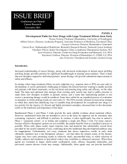
© Copyright 2026