1. sports
2. skating
3. figure skating

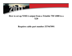
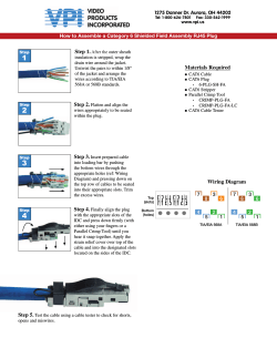
How to convert dBμV/m test results into Effective Isotropic
Radiated Power (EIRP)
How to use a CCC01 to measure cable shielding effectiveness
Test results for the radiated signal performance of
York EMC Services’ reference signal generators are
supplied in terms of the electric field strength, the
units of which are dBμV/m, as this is the common
measurement used for EMC emissions tests.
being transmitted in all directions, the EIRP is much higher
than the actual input power, which in turn leads to the gain
characteristic of the antenna. As such, the EIRP calculated
for a non-isotropic antenna is valid only for the particular
relationship between transmit and receive antennas used
to make the measurement.
The CCC01 is based on the design described in
IEC 96-1 Amendment 2:1993, also used in IEC
62153-4-6:2006 and mandated for the line injection
method in EN 50289-1-6.
In some cases, for example antenna link calculations, it can
be useful to know what the effective isotropic radiated power
(EIRP) is. This is a measurement of the power radiated
from the source and it can be derived, given a couple of
assumptions, from the value given for the electric field
strength.
So, making the assumption that the source is transmitting
equally in all directions, the power reaching any point on
the sphere described by the measurement distance is;
4
r
2
Where P is measured in watts and r
Procedure
The first assumption relates to the measurement
environment, namely that it is occurring in free space.
Reflections from nearby objects, or the attenuation of the
signal by anything other than distance, are not accounted
for. A good Fully Anechoic Room (FAR) gives this kind
of environment, an Open Area Test Site (OATS) less so
because of complications like ground-plane reflections.
With this in mind, the basic situation is shown in Figure 1.
3m in this case.
The power density is also defined by the field strength E and
the free-space impedance Z0;
E2
Z0
Pd
where E is measured in V/m and Z0
3771.
120 or approximately
Combining these two gives;
r
4
E2
120
2
E2
4
120
E2
which rearranged to;
simplifying to;
2
0.3
E2
10 log E2
20 log E
Description of the line injection
method
0.3
A schematic diagram of the line injection method is shown
in Figure 2. This is the simplest method of achieving the
theoretical arrangement described above.
1012
0.3
10 log
30
E
High quality microwave cables with N-type connectors
are needed to connect the network analyser to the CCC01.
Unwanted coupling through the screens of low quality
coaxial cables may affect the measurement. Similarly,
good quality 501 loads are needed.
The measurement of a 501 coaxial cable is described here.
Cables with different characteristic impedances can be
measured, but require special consideration.
fmax
Lmax
ഖr2
ഖr1
where;
tഖr1 is the relative permittivity of the dielectric of the
injection circuit;
tഖr2 is the relative permittivity of the cable dielectric;
t refers to near/far end measurement (+near, -far);
t is the velocity of light, 3 ×108 m/s;
1012
t fmax is the highest frequency to be measured in Hz;
E
E
The measurement of Z T is most easily achieved by using
a Network Analyser. For example an Agilent 8753ES 30kHz
to 6GHz model gives a dynamic range ~100dB (allowing
~100dB of shielding to be measured without using additional
amplifiers) and high immunity to external noise sources.
The optional time domain upgrade also allows the reflection
factor of the CCC01 “launchers” to be measured easily.
Figure 1. Theoretical arrangement for measuring ZT
0.3
1012
P
10 log
Required test instrumentation
The CCC01 can be configured to provide a coupling length
of either 0.5m or 0.3m. The standards provide a formula
for calculating the maximum cable length for a given
frequency, based on the assumption that the sample must
be electrically short at the frequency of interest. For IEC
62153-4-6:2006 the formula is:
32
E
This highlights the second assumption made, namely that
the source is isotropic, radiating equally in all directions.
This is not the case for a CNE or CGE using their respective
standard monopole and monocone antennas, as they
produce a “doughnut”-like radiation pattern. Other antennas
exhibit their own non-isotropic radiation patterns. For
example, a horn antenna has a highly focussed beamwidth
which, in the case of a transmitting antenna, concentrates
the power entering it over a small fraction of the total area
of the theoretical sphere illustrated above. In this case,
because it would be assumed that the same power is
VL (longitudinal voltage) is the voltage between points 1 and
2 on the inner conductor (Figure 1). I SH is the shield current
and L is the coupled length. As it is impractical to measure
VL directly the voltage measurement is made across the
load impedance as indicated. Normally values of Z T are
given in W/m.
0.3
E
106
Figure 1. Basic relationship between radiated power
and field strength Where P power (W), E electric
field strength (V/m) and Pd power density (W/m2)
EN 50289-1-6:2002 states “The transfer impedance Z T of an
electrically short uniform cable is defined as the quotient of
longitudinal voltage induced in the outer circuit due to the
current in the inner circuit or vice versa, related to unit length”.
York EMC Services Ltd has historically measured Z T
“vice versa”, and this method will be described here.
The transfer impedance definition can be summarised as:
To ensure both inner and outer circuits of the line injection
arrangement are matched, the transmission line comprising
the outer injection wire and the screen under test must have
a characteristic impedance (Z0) of Z OUTER. Similarly, Z 0 for the
transmission line of the screen under test and the inner pick
up conductor should equal Z INNER.
tLmax is the maximum coupled length in m.
125.2
For example assuming a relative permittivity of the cable
jacket (ഖr1) of 2.7 (pure PVC) and a relative permittivity of the
cable inner dielectric (ഖr1) of 3.8 (pure Nylon), the results of
the calculation are summarised in Table 1.
1
95.2
Theoretical fmax
In summary, bearing in mind the assumptions being made,
the Effective Isotropic Radiated Power can be derived from
the 3m field strength test measurements supplied with the
CNE and CGE reference sources by subtracting 95.2 from
the numerical value given in dBμV/m. By following the same
process for the case of 10m test measurements, 84.8 should
be subtracted instead.
www.yorkemc.co.uk
Lmax = 0.3m
Lmax = 0.5m
Near end measurements
88.6MHz
53.2MHz
Far end measurements
1.04GHz
623.7MHz
Figure 2. Schematic diagram of line injection method
Table 1. fmax vs Lmax, from IEC 62153-4-6:2006
www.yorkemc.co.uk
In practice one of the features of the jig is that samples can
be electrically long, with little standing wave disturbance for
far end measurements, so calculated values of electrical
length are not as important as suggested by the standards.
Slightly improved return loss on the injection circuit might
be obtained for a 0.3m sample, whereas a 0.5m sample
gives increased coupling. For well screened cables the
latter makes the measurement dynamic range requirements
slightly less onerous. In this example a coupled length of
0.5m is used, requiring a 1m test cable terminated with
N-type connectors.
The preparation of the test cable is covered in detail in the
CCC01 Operation Manual. Once the test cable is fitted into
the CCC01, the injection circuit must be added and this is
most easily implemented by attaching adhesive copper
foil to the test cable jacket.
Example measurements
According to IEC 62153-4-6:2006 the injection circuit should
be matched to give a return loss of better than 20dB (i.e. a
reflection factor at each launcher <0.1). This is achievable for
frequencies up to a few hundred MHz, but by 1GHz this is not
possible. Figure 5 shows typical return loss measurements
on the outer injection and the inner circuits. If available on
the network analyser, the time transform option can be used
to locate the regions where mismatch is the greatest and if
appropriate, improvements can made by altering the copper
tape width or height.
IEC 62153-4-6:2006 requires that both near and far end
measurements are made. However, as shown in Figure
7 and discussed later, for high frequency measurements
(above 50MHz) it is likely that near end measurements will
have too much resonant structure to be valid. In such cases
it is reasonable to measure Z T above 50MHz using far end
measurements only.
ZTE from S21 in accordance with
IEC 62153-4-6:2006
Equation (17) of IEC 62153-4-6:2006 states:
2R2
Lc km
20 log10
For IEC 62153-4-6:2006 at least four measurements should
be made, with the test cable rotated in the clamp each time
(i.e. 0°, 90°, 180°, 270°). This is to identify any seams in the
shield, as would occur with a foil shield.
Figure 3. Prepared test sample with injection strip
377
ഖ Z0
2
This gives a strip width of 2.5mm for ‫ڞ‬r = 2.7 (PVC) and
Z 0 = 501. It should be noted that the text book value of ‫ڞ‬r
given for PVC is unlikely to be correct due to variations in
manufacturing processes and polymer “recipes”.
R2
LC
km
The network analyser measurements of S21 can be used to
derive Z TE (Equivalent Transfer Impedance).
Measurements of coupling can be made at the “near” end
or far “end”. Figure 6 shows the CCC01 configured for a
near end measurement. Figure 7 shows the raw results for
near and far end coupling measurements. As can be seen,
the far end measurements are generally greater than those
at the near end, and furthermore are generally free from
major disturbance from standing wave effects.
Z T is a measurement of inductive coupling. If the shield is
loosely braided then some capacitive coupling will also be
measured. The inductive and capacitive parts of the coupling
cannot be separated so the standards define the parameter
Z TE that comprises both inductive and capacitive coupling
(should it be present). IEC 62153-4-6:2006 requires that
results give Z TE in units of ohms per unit length.
Urec
501 (load resistance)
0.5m (the coupled length)
1 (matching network voltage gain
in our example so km 1)
nonexistent
Expressing Equation (17) in dB for our example:
S21
Treatment of Results
Measurements of coupling
Ugen
Ugen is shown on Figure 2 and Urec corresponds to VOUTFAR
or VOUTNEAR on that diagram.
Figure 5. Injection (outer) and inner circuit return loss
Once the width of the injection strip is decided it should be
fitted and soldered to the wires protruding from the launchers
as shown in Figure 4.
Figure 4. Injection strip fitted
to Cable Under Test (CUT)
20
where for our example 501 coaxial cable
Figure 7. Typical coupling measurement results using
log frequency scale as per IEC 62153-4-6:2006
The characteristic impedance of the injection circuit is
adjusted by altering the foil strip width. For guidance, the
following formula derived from Kraus is useful, where
W = width of strip and H = height above shield, normally
~1mm for a typical cable jacket):
10
Urec
Ugen
Due to the definition of S21:
S21
Thus:
Urec
Ugen
S21
46
So to express Z TE in line with IEC 62153-4-6:2006 for the
example 0.5m long 501 coaxial cable, add 46dB to the
S21 measurement.
Figure 6. CCC01 configured for a “near”
end coupling measurement
www.yorkemc.co.uk
www.yorkemc.co.uk
53