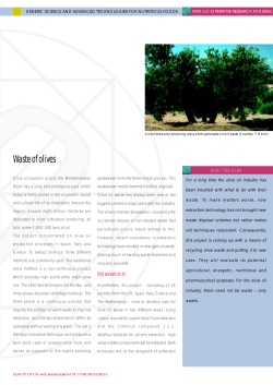
UMN TH 1427/96
astro-ph/9605068
May 1996
WHY DO WE NEED NON-BARYONIC DARK MATTER?
1
Keith A. Olive
School of Physics and Astronomy, University of Minnesota,
Minneapolis, MN 55455, USA
Abstract
Observational evidence along with theoretical arguments which call for non-baryonic dark matter are reviewed. A brief summary of the dark matter session is included.
There is increasing evidence that relative to the visible matter in the Universe, which is
in the form of baryons, there is considerably more matter in the Universe that we don’t see
[1]. Here, I will review some of the motivations for dark matter in the Universe. The best
observational evidence is found on the scale of galactic halos and comes from the observed flat
rotation curves of galaxies. There is also mounting evidence for dark matter in elliptical galaxies
as well as clusters of galaxies coming from X-ray observations of these objects. Also, direct
evidence has been obtained through the study of gravitational lenses. In theory, we believe there
is much more matter because 1) inflation tells us so (and there is at present no good alternative
to inflation) and 2) our current understanding of galaxy formation only makes sense if there is
more matter than we see. One can also make a strong case for the existence of non-baryonic
dark matter in particular. The recurrent problem with baryonic dark matter is that not only
is it very difficult to hide baryons, but the standard model of primordial nucleosynthesis would
have to discarded if all of the dark matter is baryonic. Fortunately, as will be covered at length
in these proceedings, there are several attractive alternatives to baryonic dark matter.
Before embarking on the subject of dark matter, it will be useful to review the relevant
quantities from the standard big bang model. In a Friedmann-Robertson-Walker Universe, the
expansion rate of the Universe (the Hubble parameter) is related to the energy density ρ and
curvature constant k by
!2
R˙
8πG
k
2
=
ρ− 2
(1)
H =
R
3
R
1
To be published in the proceedings of the XXXIst Recontres de Moriond, Les Arcs, France, January 20-27
1996.
1
assuming no cosmological constant, where k ±1, 0 for a closed, open or spatially flat Universe,
and R is the cosmological scale factor. When k = 0, the energy density takes its “critical” value,
ρ = ρc = 3H 2 /8πG = 1.88 × 10−29 h2o g cm−3 where ho = Ho /100 km s−1 Mpc−1 is the scaled
present value of the Hubble parameter. The cosmological density parameter is defined by
Ω = ρ/ρc and by rewriting eq. (1) we can relate k to Ω and H by
k
= (Ω − 1)H 2
R2
(2)
so that k = +1, −1, 0 corresponds to Ω > 1, < 1, = 1.
In very broad terms, observational limits on the cosmological parameters are: 0.2 <
∼Ω<
∼2
and 0.4 <
∼ 1.0 [2]. The cosmological density is however sensitive to the particular scale
∼ ho <
being observed (at least on small scales). Accountably visible matter contributes in total only
a small fraction to the overall density, giving ΩV ∼ .003 − .01. In the bright central parts of
galaxies, the density is larger Ω ∼ 0.02− 0.1. On larger scales, that of binaries and small groups
of galaxies, Ω ' 0.05 − 0.3. On even larger scales the density may be large enough to support
Ω ' 1.0. Though there are no astronomical observations to support Ω > 1, limits based on the
deceleration of the Universe only indicate [2] that Ω <
∼ 2.
The age of the Universe is also very sensitive to these parameters. Again, in the absence
of a cosmological constant we have,
Z
Ho tU =
0
1
(1 − Ω + Ω/x)−1/2 dx
(3)
For tU > 13 Gyr, Ωh2o < 0.25 if ho > 0.5 and Ωh2o < 0.45 if ho > 0.4. While for tU > 10 Gyr,
Ωh2o < 0.8 if ho > 0.5 and Ωh2o < 1.1 if ho > 0.4.
There is, in fact, good evidence for dark matter on the scale of galaxies (and their halos).
Assuming that galaxies are in virial equilibrium, one expects that by Newton’s Laws one can
relate the mass at a given distance r, from the center of a galaxy to its rotational velocity
M(r) ∝ v 2r/GN
(4)
The rotational velocity, v, is measured [3, 4, 5] by observing 21 cm emission lines in HI regions
(neutral hydrogen) beyond the point where most of the light in the galaxy ceases. A compilation
of nearly 1000 rotation curves of spiral galaxies have been plotted in [6] as a function of r for
varying brightnesses. If the bulk of the mass is associated with light, then beyond the point
where most of the light stops M would be constant and v 2 ∝ 1/r. This is not the case, as
the rotation curves appear to be flat, i.e., v ∼ constant outside the core of the galaxy. This
implies that M ∝ r beyond the point where the light stops. This is one of the strongest pieces
of evidence for the existence of dark matter. Velocity measurements indicate dark matter in
elliptical galaxies as well [7].
Galactic rotation curves are not the only observational indication for the existence of
dark matter. X-ray emitting hot gas in elliptical galaxies also provides an important piece
of evidence for dark matter. As an example, consider the large elliptical M87. The detailed
profiles of the temperature and density of the hot X-ray emitting gas have been mapped out
[8]. By assuming hydrostatic equilibrium, these measurements allow one to determine the
overall mass distribution in the galaxy necessary to bind the hot gas. Based on an isothermal
model with temperature kT = 3keV (which leads to a conservative estimate of the total mass),
2
Fabricant and Gorenstein [8] predicted that the total mass out to a radial distance of 392 Kpc,
is 5.7 × 1013 M whereas the mass in the hot gas is only 2.8 × 1012 M or only 5% of the total.
The visible mass is expected to contribute only 1% of the total. The inferred value of Ω based
on M87 would be ∼ 0.2.
M87 is not the only example of an elliptical galaxy in which X-ray emitting hot gas is
observed to indicate the presence of dark matter. At this meeting, Foreman [9], showed several
examples of ellipiticals with large mass to light ratios. For example in the case of N4472, while
the optical observations go out to 25 kpc, the X-ray gas is seen out to 75 kpc, indicating M/L’s
of about 60 at 70 kpc and up to 90 at 100 kpc. Similar inferences regarding the existence of
dark matter can be made from the X-ray emission from small groups of galaxies [10, 11].
On very large scales, it is possible to get an estimate of Ω from the distribution of peculiar
velocities. On scales, λ, where perturbations, δ, are still small, peculiar velocities can be
expressed [12] as v ∼ HλδΩ0.6 . On these scales, measurements of the peculiar velocity field
from the IRAS galaxy catalogue indicate that indeed Ω is close to unity [13]. Another piece
of evidence on large scales, is available from gravitational lensing [14]. The systematic lensing
of the roughly 150,000 galaxies per deg2 at redshifts between z = 1 − 3 into arcs and arclets
allow one to trace the matter distribution in a foreground cluster. Van Waerbeke discussed
recent results of weak gravitational lensing looking at systems, which if virialized, have mass
to light ratios in the range 400–1000 and correspond to values of Ω between 0.25 and 0.6 [15].
Unfortunately, none of these observations reveal the identity of the dark matter.
Theoretically, there is no lack of support for the dark matter hypothesis. The standard
big bang model including inflation almost requires that Ω = 1 [16]. The simple and unfortunate
fact that at present we do not even know whether Ω is larger or smaller than one indicates that
we do not know the sign of the curvature term, further implying that it is subdominant in Eq.
(1)
k
8πG
<
ρ
(5)
2
R
3
In an adiabatically expanding Universe, R ∼ T −1 where T is the temperature of the thermal
photon background. Therefore the quantity
kˆ =
k
8πG
<
< 2 × 10−58
R2 T 2
3To2
(6)
is dimensionless and constant in the standard model. The smallness of kˆ is known as the
curvature problem and can be resolved by a period of inflation. Before inflation, let us write
R = Ri , T = Ti and R ∼ T −1. During inflation, R ∼ T −1 ∼ eHt, where H is constant. After
inflation, R = Rf Ri but T = Tf = TR <
∼ Ti where TR is the temperature to which the
−1
ˆ
Universe reheats. Thus R 6∼ T and k → 0 is not constant. But from Eqs. (2) and (6) if
kˆ → 0 then Ω → 1, and since typical inflationary models contain much more expansion than is
necessary, Ω becomes exponentially close to one.
If this is the case and Ω = 1, then we know two things: Dark matter exists, since we don’t
see Ω = 1 in luminous objects, and most (at least 90%) of the dark matter is not baryonic.
The latter conclusion is a result from big bang nucleosynthesis [17, 18], which constrains the
baryon-to-photon ratio η = nB /nγ to
1.4 × 10−10 < η < 3.8 × 10−10
3
(7)
which corresponds to a limit on ΩB
0.005 < ΩB < 0.09
(8)
for 0.4 <
∼ 1.0. Thus 1 − ΩB is not only dark but also non-baryonic. I will return to big
∼ ho <
bang nucleosynthesis below.
Another important piece of theoretical evidence for dark matter comes from the simple
fact that we are here living in a galaxy. The type of perturbations produced by inflation [19]
are, in most models, adiabatic perturbations (δρ/ρ ∝ δT /T ), and I will restrict my attention
to these. Indeed, the perturbations produced by inflation also have the very nearly scale-free
spectrum described by Harrison and Zeldovich [20]. When produced, scale-free perturbations
fall off as δρ
∝ l−2 (increase as the square of the wave number). At early times δρ/ρ grows
ρ
as t until the time when the horizon scale (which is proportional to the age of the Universe)
is comparable to l. At later times, the growth halts (the mass contained within the volume
l3 has become smaller than the Jean’s mass) and δρ
= δ (roughly) independent of the scale l.
ρ
When the Universe becomes matter dominated, the Jean’s mass drops dramatically and growth
∝ R ∼ 1/T . For an overview of the evolution of density perturbations and the
continues as δρ
ρ
resulting observable spectrum see [21]. The transition to matter dominance is determined by
setting the energy densities in radiation (photons and any massless neutrinos) equal to the
energy density in matter (baryons and any dark matter). For three massless neutrinos and
baryons (no dark matter), matter dominance begins at
Tm = 0.22mB η
(9)
and for η < 3.8 × 10−10 , this corresponds to Tm < 0.08 eV.
The subsequent non-linear growth in δρ/ρ was discussed in these sessions in some detail at
this meeting. In particular, there was a considerable discussion of the effects of the non-linear
regime on the power spectrum and the appearance of non-Gaussian features such as skewness
and kurtosis [22]. Colombi [23] discussed the 2- and 3-point correlation functions. Numerous
simulations were presented to reflect the hydrodynamics of galaxy formation [24] and the origin
of the large scale bias [25].
Because we are considering adiabatic perturbations, there will be anisotropies produced
in the microwave background radiation on the order of δT /T ∼ δ. The value of δ, the amplitude
of the density fluctuations at horizon crossing, has now been determined by COBE [26], δ =
(5.7 ± 0.4) × 10−6 . Without the existence of dark matter, δρ/ρ in baryons could then achieve
−3
−4
a maximum value of only δρ/ρ ∼ Aλδ(Tm/To ) <
∼ 2 × 10 Aλ, where To = 2.35 × 10 eV is the
present temperature of the microwave background and Aλ ∼ 1 − 10 is a scale dependent growth
factor. The overall growth in δρ/ρ is too small to argue that growth has entered a nonlinear
regime needed to explain the large value (105 ) of δρ/ρ in galaxies.
Dark matter easily remedies this dilemma in the following way. The transition to matter dominance is determined by setting equal to each other the energy densities in radiation
(photons and any massless neutrinos) and matter (baryons and any dark matter). While if we
suppose that there exists dark matter with an abundance Yχ = nχ /nγ (the ratio of the number
density of χ’s to photons) then
(10)
Tm = 0.22mχ Yχ
Since we can write mχ Yχ /GeV = Ωχ h2 /(4 × 107 ), we have Tm /To = 2.4 × 104 Ωχ h2 which is
to be compared with 350 in the case of baryons alone. The baryons, although still bound
4
to the radiation until decoupling, now see deep potential wells formed by the dark matter
perturbations to fall into and are no longer required to grow at the rate δρ/ρ ∝ R.
With regard to dark matter and galaxy formation, all forms of dark matter are not equal.
They can be distinguished by their relative temperature at Tm [27]. Particles which are still
largely relativistic at Tm (like neutrinos or other particles with mχ < 100 eV) have the property
[28] that (due to free streaming) they erase perturbations out to very large scales given by the
Jean’s mass
M
MJ = 3 × 1018 2
(11)
mν (eV )
Thus, very large scale structures form first and galaxies are expected to fragment out later.
Particles with this property are termed hot dark matter particles. Cold particles (mχ > 1
MeV) have the opposite behavior. Small scale structure forms first aggregating to form larger
structures later. Neither candidate is completely satisfactory when the resulting structure is
compared to the observations. For more details, I refer the reader to reviews in refs. [1].
The most promising possibility we have for unscrambling the various possible scenarios
for structure formation is the careful analysis of the observed power spectrum. Rewriting the
density contrast in Fourier space,
δ(k) ∝
Z
d3 x
δρ
(x)eik·x
ρ
(12)
the power spectrum is just
P (k) = h|δ(k)|2i
(13)
which is often written in term of a transfer function and a power law, P ∼ T (k)k n . (The flat
spectrum produced by inflation has n = 1.) The data contributing to P (k) include observations
of galaxy distributions, velocity distributions and of course the CMB [29]. However to make a
comparison with our theoretical expectations, we rely on n-body simulations and a deconvolution of the theory from the observations. Overall, there is actually a considerable amount of
concordance with our expectations. The velocity distributions indicate that 0.3 < Ω < 1 and
the power spectrum is roughly consistent with an Ω = 1, and n = 1, cold dark matter Universe.
Future surveys [30, 31] will however, most certainly dramatically improve our understanding of the detailed features of the power spectrum and their theoretical interpretations. We
should in principle be able to distinguish between a mixed dark matter and a cold dark matter
Ω = 1 Universe, whether or not Ω < 1, with CDM, the presence of a cosmological constant,
or a tilt in the spectrum. Zurek [32], stressed the importance of numerical simulations in this
context. Future probes of the small scale anisotropy [31, 33] should in addition be able to
determine the values of not only Ω, but also ΩB and ho to a high degree of accuracy through a
careful analysis of the Doppler peak in the power spectrum.
Accepting the dark matter hypothesis, the first choice for a candidate should be something
we know to exist, baryons. Though baryonic dark matter can not be the whole story if Ω = 1,
the identity of the dark matter in galactic halos, which appear to contribute at the level of
Ω ∼ 0.05, remains an important question needing to be resolved. A baryon density of this
magnitude is not excluded by nucleosynthesis. Indeed we know some of the baryons are dark
since Ω <
∼ 0.01 in the disk of the galaxy.
It is quite difficult, however, to hide large amounts of baryonic matter [34]. Sites for halo
baryons that have been discussed include snowballs, which tend to sublimate, cold hydrogen
5
gas, which must be supported against collapse, and hot gas, which can be excluded by the
X-ray background. Stellar objects (collectively called MACHOs for macroscopic compact halo
objects) must either be so small ( M < 0.08 M) so as not to have begun nuclear burning or
so massive so as to have undergone total gravitational collapse without the ejection of heavy
elements. Intermediate mass stars are generally quite problematic because either they are
expected to still reside on the main-sequence today and hence would be visible, or they would
have produced an excess of heavy elements.
On the other hand, MACHOs are a candidate which are testable by the gravitational
microlensing of stars in a neighboring galaxy such as the LMC [35]. By observing millions
of stars and examining their intensity as a function of time, it may be possible to determine
the presence of dark objects in our halo. It is expected that during
q a lensing event, a star’s
intensity will rise in an achromatic fashion over a period δt ∼ 3 M/.001M days. Indeed,
microlensing candidates have been found [36]. For low mass objects, those with M < 0.1M ,
it appears however that the halo fraction of Machos is small, ≈ 0.19+.16
−.10 [37]. There have been
some recent reports of events with longer duration [38] leading to the speculation of a white
dwarf population in the halo. Though it is too early to determine the implications of these
observations, they are very encouraging in that perhaps this issue can and will be decided.
The degree to which baryons can contribute to dark matter depends ultimately on the
overall baryon contribution to Ω which is constrained by nucleosynthesis. Because of its importance regarding the issue of dark matter and in particular non-baryonic dark matter, I want to
review the status of big bang nucleosynthesis.
Conditions for the synthesis of the light elements were attained in the early Universe at
temperatures T <
∼ 1 MeV, corresponding to an age of about 1 second. Given a single input
parameter, the baryon-to-photon ratio, η, the theory is capable of predicting the primordial
abundances of D/H, 3 He/H, 4 He/H and 7Li/H. The comparison of these predictions with the
observational determination of the abundances of the light elements not only tests the theory
but also fixes the value of η.
The dominant product of big bang nucleosynthesis is 4 He resulting in an abundance of
close to 25 % by mass. In the standard model, the 4 He mass fraction depends only weakly on
η. When we go beyond the standard model, the 4He abundance is very sensitive to changes
in the expansion rate which can be related to the effective number of neutrino flavors. Lesser
amounts of the other light elements are produced: D and 3 He at the level of about 10−5 by
number, and 7 Li at the level of 10−10 by number.
There is now a good collection of abundance information on the 4 He mass fraction, Y ,
O/H, and N/H in over 50 extragalactic HII (ionized hydrogen) regions [39, 40, 41]. The observation of the heavy elements is important as the helium mass fraction observed in these HII
regions has been augmented by some stellar processing, the degree to which is given by the
oxygen and nitrogen abundances. In an extensive study based on the data in [39, 40], it was
found [42] that the data is well represented by a linear correlation for Y vs. O/H and Y vs.
N/H. It is then expected that the primordial abundance of 4 He can be determined from the
intercept of that relation. The overall result of that analysis indicated a primordial mass fraction, Yp = 0.232 ± 0.003. In [43], the stability of this fit was verified by a Monte-Carlo analysis
showing that the fits were not overly sensitive to any particular HII region. In addition, the
data from [41] was also included, yielding a 4He mass fraction [43]
Yp = 0.234 ± 0.003 ± 0.005
6
(14)
The second uncertainty is an estimate of the systematic uncertainty in the abundance determi
nation.
The 7 Li abundance is also reasonably well known. In old, hot, population-II stars, 7Li
is found to have a very nearly uniform abundance. For stars with a surface temperature
T > 5500 K and a metallicity less than about 1/20th solar (so that effects such as stellar
convection may not be important), the abundances show little or no dispersion beyond that
which is consistent with the errors of individual measurements. Indeed, as detailed in [44], much
of the work concerning 7 Li has to do with the presence or absence of dispersion and whether
or not there is in fact some tiny slope to a [Li] = log 7Li/H + 12 vs. T or [Li] vs. [Fe/H]
relationship. There is 7 Li data from nearly 100 halo stars, from a variety of sources. I will
use the value given in [45] as the best estimate for the mean 7 Li abundance and its statistical
uncertainty in halo stars
+1.6
−10
Li/H = (1.6 ± 0.1+0.4
(15)
−0.3 −0.5 ) × 10
The first error is statistical, and the second is a systematic uncertainty that covers the range
of abundances derived by various methods. The third set of errors in Eq. (15) accounts for
the possibility that as much as half of the primordial 7 Li has been destroyed in stars, and that
as much as 30% of the observed 7Li may have been produced in cosmic ray collisions rather
than in the Big Bang. Observations of 6 Li, Be, and B help constrain the degree to which these
effects play a role [46]. For 7 Li, the uncertainties are clearly dominated by systematic effects.
Turning to D/H, we have three basic types of abundance information: 1) ISM data,
2) solar system information, and perhaps 3) a primordial abundance from quasar absorption
systems. The best measurement for ISM D/H is [47]
−5
(D/H)ISM = 1.60 ± 0.09+0.05
−0.10 × 10
(16)
This value may not be universal (or galactic as the case may be) since there may be some real
dispersion of D/H in the ISM [48]. The solar abundance of D/H is inferred from two distinct
measurements of 3 He. The solar wind measurements of 3 He as well as the low temperature
components of step-wise heating measurements of 3 He in meteorites yield the presolar (D +
3
He)/H ratio, as D was efficiently burned to 3He in the Sun’s pre-main-sequence phase. These
measurements indicate that [49, 50]
D + 3 He
H
!
= (4.1 ± 0.6 ± 1.4) × 10−5
(17)
The high temperature components in meteorites are believed to yield the true solar 3 He/H ratio
of [49, 50]
!
3
He
= (1.5 ± 0.2 ± 0.3) × 10−5
(18)
H The difference between these two abundances reveals the presolar D/H ratio, giving,
(D/H) ≈ (2.6 ± 0.6 ± 1.4) × 10−5
(19)
Finally, there have been several recent reported measurements of D/H is high redshift quasar
absorption systems. Such measurements are in principle capable of determining the primordial
value for D/H and hence η, because of the strong and monotonic dependence of D/H on η.
However, at present, detections of D/H using quasar absorption systems indicate both a high
7
and low value of D/H. As such, we caution that these values may not turn out to represent
the true primordial value. The first of these measurements [51] indicated a rather high D/H
ratio, D/H ≈ 1.9 – 2.5 ×10−4 . A recent re-observation of the high D/H absorption system has
been resolved into two components, both yielding high values with an average value of D/H =
−4
1.9+0.4
[52] as well as an additional system with a similar high value [53]. Other high
−0.3 × 10
D/H ratios were reported in [54]. However, there are reported low values of D/H in other such
systems [55] with values D/H ' 2.5 × 10−5 , significantly lower than the ones quoted above. It
is probably premature to use this value as the primordial D/H abundance in an analysis of big
bang nucleosynthesis, but it is certainly encouraging that future observations may soon yield
a firm value for D/H. It is however important to note that there does seem to be a trend that
over the history of the Galaxy, the D/H ratio is decreasing, something we expect from galactic
chemical evolution. Of course the total amount of deuterium astration that has occurred is still
uncertain, and model dependent.
There are also several types of 3 He measurements. As noted above, meteoritic extractions
yield a presolar value for 3 He/H as given in Eq. (18). In addition, there are several ISM
measurements of 3 He in galactic HII regions [56] which also show a wide dispersion
3
He
H
!
' 1 − 5 × 10−5
(20)
HII
There is also a recent ISM measurement of 3 He [57] with
3
He
H
!
−5
= 2.1+.9
−.8 × 10
(21)
ISM
Finally there are observations of 3He in planetary nebulae [58] which show a very high 3 He
abundance of 3 He/H ∼ 10−3 .
Each of the light element isotopes can be made consistent with theory for a specific range
in η. Overall consistency of course requires that the range in η agree among all four light
elements. 3He (together with D) has stood out in its importance for BBN, because it provided
a (relatively large) lower limit for the baryon-to-photon ratio [59], η10 > 2.8. This limit for
a long time was seen to be essential because it provided the only means for bounding η from
below and in effect allows one to set an upper limit on the number of neutrino flavors [60],
Nν , as well as other constraints on particle physics properties. That is, the upper bound to
Nν is strongly dependent on the lower bound to η. This is easy to see: for lower η, the 4 He
abundance drops, allowing for a larger Nν , which would raise the 4 He abundance. However,
for η < 4 × 10−11 , corresponding to Ωh2 ∼ .001 − .002, which is not too different from galactic
mass densities, there is no bound whatsoever on Nν [61]. Of course, with the improved data
on 7 Li, we do have lower bounds on η which exceed 10−10 .
In [59], it was argued that since stars (even massive stars) do not destroy 3He in its
entirety, we can obtain a bound on η from an upper bound to the solar D and 3He abundances.
One can in fact limit [59, 62] the sum of primordial D and 3 He by applying the expression below
at t = !
!
D + 3He
D
1 3He
≤
+
(22)
H
H t g3 H t
p
In (22), g3 is the fraction of a star’s initial D and 3He which survives as 3 He. For g3 > 0.25 as
suggested by stellar models, and using the solar data on D/H and 3 He/H, one finds η10 > 2.8.
8
The limit η10 > 2.8 derived using (22) is really a one shot approximation. Namely, it
is assumed that material passes through a star no more than once. To determine whether
or not the solar (and present) values of D/H and 3 He/H can be matched it is necessary to
consider models of galactic chemical evolution [63]. In the absence of stellar 3He production,
particularly by low mass stars, it was shown [64] that there are indeed suitable choices for a star
formation rate and an initial mass function to: 1) match the D/H evolution from a primordial
value (D/H)p = 7.5 × 10−5 , corresponding to η10 = 3, through the solar and ISM abundances,
while 2) at the same time keeping the 3He/H evolution relatively flat so as not to overproduce
3
He at the solar and present epochs. This was achieved for g3 > 0.3. Even for g3 ∼ 0.7, the
present 3 He/H could be matched, though the solar value was found to be a factor of 2 too high.
For (D/H)p ' 2 × 10−4 , corresponding to η10 ' 1.7, models could be found which destroy D
sufficiently; however, overproduction of 3 He occurred unless g3 was tuned down to about 0.1.
In the context of models of galactic chemical evolution, there is, however, little justification
a priori for neglecting the production of 3 He in low mass stars. Indeed, stellar models predict
that considerable amounts of 3 He are produced in stars between 1 and 3 M. For M < 8M ,
Iben and Truran [65] calculate
−4
( He/H)f = 1.8 × 10
3
M
M
2
h
i
+ 0.7 (D + 3 He)/H
i
(23)
so that at η10 = 3, and ((D + 3 He)/H)i = 9 × 10−5 , g3 (1M) = 2.7! It should be emphasized
that this prediction is in fact consistent with the observation of high 3 He/H in planetary nebulae
[58].
Generally, implementation of the 3 He yield in Eq. (23) in chemical evolution models
leads to an overproduction of 3 He/H particularly at the solar epoch [66, 67]. In Figure 1, the
evolution of D/H and 3 He/H is shown as a function of time from [49, 66]. The solid curves
show the evolution in a simple model of galactic chemical evolution with a star formation rate
proportional to the gas density and a power law IMF (see [66]) for details). The model was
chosen to fit the observed deuterium abundances. However, as one can plainly see, 3 He is grossly
overproduced (the deuterium data is represented by squares and 3He by circles). Depending
on the particular model chosen, it may be possible to come close to at least the upper end of
the range of the 3 He/H observed in galactic HII regions [56], although the solar value is missed
by many standard deviations.
The overproduction of 3 He relative to the solar meteoritic value seems to be a generic
feature of chemical evolution models when 3 He production in low mass stars is included. In
[49], a more extreme model of galactic chemical evolution was tested. There, it was assumed
that the initial mass function was time dependent in such a way so as to favor massive stars early
on (during the first two Gyr of the galaxy). Massive stars are preferential from the point of view
of destroying 3He. However, massive stars are also proficient producers of heavy elements and
in order to keep the metallicity of the disk down to acceptable levels, supernovae driven outflow
was also included. The degree of outflow was limited roughly by the observed metallicity in
the intergalactic gas in clusters of galaxies. One further assumption was necessary; we allowed
the massive stars to lose their 3 He depleted hydrogen envelopes prior to explosion. Thus
only the heavier elements were expulsed from the galaxy. With all of these (semi-defensible)
assumptions, 3 He was still overproduced at the solar epoch, as shown by the dashed curve in
Figure 1. Though there certainly is an improvement in the evolution of 3He without reducing
the yields of low mass stars, it is hard to envision much further reduction in the solar 3 He
9
10
8
6
4
2
0
0
5
10
15
Figure 1: The evolution of D and 3 He with time.
predicted by these models. The only conclusion that we can make at this point is that there is
clearly something wrong with our understanding of 3 He in terms of either chemical evolution,
stellar evolution or perhaps even the observational data.
Given the magnitude of the problems concerning 3 He, it would seem unwise to make any
strong conclusion regarding big bang nucleosynthesis which is based on 3 He. Perhaps as well
some caution is deserved with regard to the recent D/H measurements, although if the present
trend continues and is verified in several different quasar absorption systems, then D/H will
certainly become our best measure for the baryon-to-photon ratio. Given the current situation
however, it makes sense to take a step back and perform an analysis of big bang nucleosynthesis
in terms of the element isotopes that are best understood, namely 4 He and 7Li.
Monte Carlo techniques are proving to be a useful form of analysis for big bang nucleosynthesis [68, 69]. In [18], we performed just such an analysis using only 4 He and 7 Li. It
should be noted that in principle, two elements should be sufficient for constraining the one
parameter (η) theory of BBN. We begin by establishing likelihood functions for the theory and
observations. For example, for 4 He, the theoretical likelihood function takes the form
LBBN (Y, YBBN) = e−(Y −YBBN (η))
2
/2σ12
(24)
where YBBN (η) is the central value for the 4He mass fraction produced in the big bang as
predicted by the theory at a given value of η, and σ1 is the uncertainty in that value derived
from the Monte Carlo calculations [69] and is a measure of the theoretical uncertainty in
the big bang calculation. Similarly one can write down an expression for the observational
likelihood function. In this case we have two sources of errors, as discussed above, a statistical
uncertainty, σ2 and a systematic uncertainty, σsys. Here, I will assume that the systematic error
is described by a top hat distribution [69, 70]. The convolution of the top hat distribution and
the Gaussian (to describe the statistical errors in the observations) results in the difference of
10
0.9
0.8
0.7
0.6
0.5
0.4
0.3
0.2
0.1
0.0
0.00
2.00
4.00
6.00
8.00
10.00
η10
Figure 2: Likelihood distribution for each of 4 He and 7Li, shown as a function of η. The
one-peak structure of the 4He curve corresponds to its monotonic increase with η, while the
two-peaks for 7 Li arise from its passing through a minimum.
two error functions
Y − YO + σsys
√
LO (Y, YO) = erf
2σ2
!
Y − YO − σsys
√
− erf
2σ2
!
(25)
where in this case, YO is the observed (or observationally determined) value for the 4 He mass
fraction. (Had I used a Gaussian to describe the systematic uncertainty, the convolution of
two Gaussians leads to a Gaussian, and the likelihood function (25) would have taken a form
similar to that in (24).
A total likelihood function for each value of η10 is derived by convolving the theoretical
and observational distributions, which for 4 He is given by
4 He
L
Z
total(η) =
dY LBBN (Y, YBBN (η)) LO(Y, YO )
(26)
An analogous calculation is performed [18] for 7 Li. The resulting likelihood functions from the
observed abundances given in Eqs. (14) and (15) is shown in Figure 2. As one can see there is
very good agreement between 4 He and 7Li in the vicinity of η10 ' 1.8.
The combined likelihood, for fitting both elements simultaneously, is given by the product
of the two functions in Figure 2 and is shown in Figure 3. From Figure 2 it is clear that
4
He overlaps the lower (in η) 7 Li peak, and so one expects that there will be concordance
in an allowed range of η given by the overlap region. This is what one finds in Figure 3,
which does show concordance and gives a preferred value for η, η10 = 1.8+1
−.2 corresponding to
+.004
2
ΩB h = .006−.001 .
Thus, we can conclude that the abundances of 4 He and 7Li are consistent, and select
an η10 range which overlaps with (at the 95% CL) the longstanding favorite range around
η10 = 3. Furthermore, by finding concordance using only 4He and 7Li, we deduce that if there
11
0.400
0.300
0.200
0.100
0.000
0.00
2.00
4.00
6.00
8.00
10.00
η10
Figure 3: Combined likelihood for simultaneously fitting 4He and 7Li, as a function of η.
is problem with BBN, it must arise from D and 3He and is thus tied to chemical evolution or the
stellar evolution of 3 He. The most model-independent conclusion is that standard BBN with
Nν = 3 is not in jeopardy, but there may be problems with our detailed understanding of D and
particularly 3 He chemical evolution. It is interesting to note that the central (and strongly)
peaked value of η10 determined from the combined 4 He and7 Li likelihoods is at η10 = 1.8.
The corresponding value of D/H is 1.8 ×10−4 , very close to the high value of D/H in quasar
absorbers [51, 52, 54]. Since D and 3 He are monotonic functions of η, a prediction for η, based
on 4 He and 7Li, can be turned into a prediction for D and 3He. The corresponding 95% CL
ranges are D/H = (5.5 − 27) × 10−5 and and 3He/H = (1.4 − 2.7) × 10−5 .
If we did have full confidence in the measured value of D/H in quasar absorption systems,
then we could perform the same statistical analysis using 4 He, 7 Li, and D. To include D/H,
one would proceed in much the same way as with the other two light elements. We compute
likelihood functions for the BBN predictions as in Eq. (24) and the likelihood function for the
observations using D/H = (1.9 ± 0.4) × 10−4 . We are using only the high value of D/H here.
These are then convolved as in Eq. (26). In figure 4, the resulting normalized distribution,
LD
total (η) is super-imposed on distributions appearing in figure 2. It is indeed startling how the
three peaks, for D, 4 He and 7 Li are literally on top of each other. In figure 5, the combined
distribution is shown. We now have a very clean distribution and prediction for η, η10 = 1.75+.3
−.1
+.001
2
corresponding to ΩB h = .006−.0004, with the peak of the distribution at η10 = 1.75. The
absence of any overlap with the high-η peak of the 7 Li distribution has considerably lowered
the upper limit to η. Overall, the concordance limits in this case are dominated by the deuterium
likelihood function.
To summarize on the subject of big bang nucleosynthesis, I would assert that one can
conclude that the present data on the abundances of the light element isotopes are consistent
with the standard model of big bang nucleosynthesis. Using the the isotopes with the best
data, 4 He and 7Li, it is possible to constrain the theory and obtain a best value for the baryon12
1.6
1.4
1.2
1.0
0.8
0.6
0.4
0.2
0.0
0.00
2.00
4.00
6.00
8.00
10.00
η10
Figure 4: As in Figure 2, with the addition of the likelihood distribution for D/H.
0.500
0.400
0.300
0.200
0.100
0.000
0.00
2.00
4.00
6.00
8.00
10.00
η10
Figure 5: Combined likelihood for simultaneously fitting 4 He and 7Li, and D as a function of η.
13
to photon ratio of η10
1.8, a corresponding value ΩB
1.4
< η10
< 3.8
.005 < ΩB h2 < .014
.0065 and
95%CL
95%CL
(27)
For 0.4 < h < 1, we have a range .005 < ΩB < .09. This is a rather low value for the baryon
density and would suggest that much of the galactic dark matter is non-baryonic [71]. These
predictions are in addition consistent with recent observations of D/H in quasar absorption
systems which show a high value. Difficulty remains however, in matching the solar 3 He abundance, suggesting a problem with our current understanding of galactic chemical evolution or
the stellar evolution of low mass stars as they pertain to 3 He.
If we now take as given that non-baryonic dark matter is required, we are faced with the
problem of its identity. Light neutrinos (m ≤ 30eV ) are a long-time standard when it comes
to non-baryonic dark matter [72]. Light neutrinos produce structure on large scales and the
natural (minimal) scale for structure clustering is given in Eq. (11). Hence neutrinos offer the
natural possibility for large scale structures [73, 74] including filaments and voids. It seemed,
however, that neutrinos were ruled out because they tend to produce too much large scale
structure [75]. Because the smallest non-linear structures have mass scale MJ and the typical
galactic mass scale is ' 1012 M , galaxies must fragment out of the larger pancake-like objects.
The problem is that in such a scenario, galaxies form late [74, 76] (z ≤ 1) whereas quasars and
galaxies are seen out to redshifts z >
∼ 4. Recently, neutrinos are seeing somewhat of a revival
in popularity in mixed dark matter models.
In the standard model, the absence of a right-handed neutrino state precludes the existence
of a neutrino mass. By adding√a right-handed state νR , it is possible to generate a Dirac mass
for the neutrino, mν = hν v/ 2, as for the charged lepton masses, where hν is the neutrino
Yukawa coupling constant, and v is the Higgs expectation value. It is also possible to generate
a Majorana mass for the neutrino when in addition to the Dirac mass term, mν ν¯R νL , a term
MνR νR is included. In what is known as the see-saw mechanism, the two mass eigenstates are
given by mν1 ∼ m2ν /M which is very light, and mν2 ∼ M which is heavy. The state ν1 is our
hot dark matter candidate as ν2 is in general not stable.
The cosmological constraint on the mass of a light neutrino is derived from the overall
mass density of the Universe. In general, the mass density of a light particle χ can be expressed
as
ρχ = mχ Yχ nγ ≤ ρc = 1.06 × 10−5 ho 2 GeV/cm3
(28)
where Yχ = nχ /nγ is the density of χ’s relative to the density of photons, for Ωho 2 < 1. For
neutrinos Yν = 3/11, and one finds [77]
X
(
ν
gν
)mν < 93eV(Ωho 2 )
2
(29)
where the sum runs over neutrino flavors. All particles with abundances Y similar to neutrinos
will have a mass limit given in Eq. (29).
It was possible that neutrinos (though not any of the known flavors) could have had large
masses, mν > 1 MeV. In that case their abundance Y is controlled by ν, ν¯ annihilations [78],
for example, ν ν¯ → f f¯ via Z exchange. When the annihilations freeze-out (the annihilation
rate becomes slower than the expansion rate of the Universe), Y becomes fixed. Roughly,
Y ∼ (mσA)−1 and ρ ∼ σA −1 where σA is the annihilation cross-section. For neutrinos, we
14
expect σA
mν /mZ so that ρν
1/mν and we can derive a lower bound [79, 80] on the
neutrino mass, mν >
3
−
7
GeV,
depending
on whether it is a Dirac or Majorana neutrino.
∼
Indeed, any particle with roughly a weak scale cross-sections will tend to give an interesting
value of Ωh2 ∼ 1 [81].
Due primarily to the limits from LEP [82], the heavy massive neutrino has become simply
an example and is no longer a dark matter candidate. LEP excludes neutrinos (with standard
weak interactions) with masses mν <
∼ 40 GeV. Lab constraints for Dirac neutrinos are available
[83], excluding neutrinos with masses between 10 GeV and 4.7 TeV. This is significant, since
it precludes the possibility of neutrino dark matter based on an asymmetry between ν and ν¯
[84]. Majorana neutrinos are excluded as dark matter since Ων ho 2 < 0.001 for mν > 40 GeV
and are thus cosmologically uninteresting.
Supersymmetric theories introduce several possible candidates. If R-parity, which distinguishes between “normal” matter and the supersymmetric partners and can be defined in terms
of baryon, lepton and spin as R = (−1)3B+L+2S , is unbroken, there is at least one supersymmetric particle which must be stable. I will assume R-parity conservation, which is common
in the MSSM. R-parity is generally assumed in order to justify the absence of superpotential
terms can be responsible for rampid proton decay. The stable particle (usually called the LSP)
is most probably some linear combination of the only R = −1 neutral fermions, the neutralinos
˜ 3, the partner of the 3rd component of the SU(2)L gauge boson; the bino,
[85]: the wino W
˜ 1 and H
˜ 2 . Gluinos
˜ the partner of the U(1)Y gauge boson; and the two neutral Higgsinos, H
B,
are expected to be heavier -mg˜ = ( αα3 ) sin2 θW M2 , where M2 is the supersymmetry breaking
SU(2) gaugino mass- and they do not mix with the other states. The sneutrino [86] is also a
possibility but has been excluded as a dark matter candidate by direct [83] searches, indirect
[87] and accelerator[82] searches. For more on the motivations for supersymmetry and the
supersymmetric parameter space, see the contribution of Jungman [81].
The identity of the LSP is effectively determined by three parameter in the MSSM, the
gaugino mass, M2 , the Higgs mixing mass µ, and the ratio of the Higgs vacuum expectation
values, tan β. In Figure 6 [89], regions in the M2 , µ plane with tan β = 2 are shown in which
˜ a symmetric
the LSP is one of several nearly pure states, the photino, γ˜, the U(1) gaugino, B,
1
˜ (12) = √ (H
˜ 1 +H
˜ 2 ), or the Higgsino S˜ = H
˜ 1 cos β+H
˜ 2 sin β. The
combination of the Higgsinos, H
2
dashed lines show the LSP mass contours. The cross hatched regions correspond to parameters
˜ ±, H
˜ ±) state with mass mχ˜ ≤ 45GeV and as such are excluded by LEP[90].
giving a chargino (W
This constraint has been extended by LEP1.5, [91, 92] and is shown by the light shaded region
and corresponds to regions where the chargino mass is <
∼ 67 GeV. The dark shaded region
corresponds to a limit on M2 from the limit[93] on the gluino mass mg˜ ≤ 70 GeV or M2 ≤ 22
˜ or H
˜ 12 pure states and that the
GeV. Notice that the parameter space is dominated by the B
photino (most often quoted as the LSP) only occupies a small fraction of the parameter space,
as does the Higgsino combination S˜0.
As described in [81], the relic abundance of LSP’s is determined by solving the Boltzmann
equation for the LSP number density in an expanding Universe. The technique[80] used is
similar to that for computing the relic abundance of massive neutrinos[78]. For binos, as was
the case for photinos [88], it is possible to adjust the sfermion masses mf˜ to obtain closure
density. Adjusting the sfermion mixing parameters [95] or CP violating phases [96] allows even
greater freedom. In Figure 7 [97], the relic abundance (Ωh2 ) is shown in the M2 − µ plane with
tan β = 2, the Higgs pseudoscalar mass m0 = 50 GeV, mt = 100 GeV, and mf˜ = 200 GeV.
Clearly the MSSM offers sufficient room to solve the dark matter problem. Similar results have
15
−µ
Figure 6: The M2 -µ plane in the MSSM for tan β = 2.
˜ 12 marked off by
been found by other groups [98, 99, 100]. In Figure 7, in the higgsino sector H
˜ (12) and the next lightest neutralino (also
the dashed line, co-annihilations [101, 99] between H
a Higgsino) were not included. These tend to lower significantly the relic abundance in much
of this sector.
Though I have concentrated on the LSP in the MSSM as a cold dark matter candidate,
there are many other possibilities when one goes beyond the standard model. Axions were
discussed at length by Jungman [81] and Lu [102]. A host of other possibilities were discussed
by Khlopov [103].
The final subject that I will cover in this introduction/summary is the question of detection. Dark matter detection can be separated into two basic methods, direct [104] and indirect
[105]. Direct detection relies on the ability to detect the elastic scattering of a dark matter
candidate off a nucleus in a detector. The experimental signatures for direct detection were
covered by Cabrera [106] and several individual experiments were described [107].
The detection rate, will depend on the density of dark matter in the solar neighborhood,
ρ ∼ 0.3 GeV/cm3, the velocity, v ∼ 300 km/s, and the elastic cross section, σ. Spin independent interactions are the most promising for detection. Dirac neutrinos have spin-independent
interactions, but as noted above, these have already been excluded as dark matter by direct
detection experiments [83]. In the MSSM, it is possible for the LSP to also have spin independent interactions which are mediated by Higgs exchange. These scatterings are only important
when the LSP is a mixed (gaugino/Higgsino) state as in the central regions of Figures 6 and 7.
Generally, these regions have low values of Ωh2 (since the annihilation cross sections are also
enhanced) and the parameter space in which the elastic cross section and relic density are large
16
10000
1/
4
1
1/4
1
3000
1
1/
4
1000
1/
16
300
−µ
1/
64
1
No DM
100
1/
16
1/
4
1
No DM
30
1/
4
10
10
1/
16
30
100
300
1000
3000
10000
M2 (GeV)
Figure 7: Relic density contours (Ωh2 ) in the M2 - µ plane.
is rather limited. Furthermore, a significant detection rate in this case relies on a low mass for
the Higgs scalar [108, 109].
More typical of the SUSY parameter space is a LSP with spin dependent interactions.
Elastic scatterings are primarily spin dependent whenever the LSP is mostly either gaugino or
˜ (12)
Higgsino. For Higgsino dark matter, Higgsinos with scatterings mediated by Z 0 avoid the H
regions of Figures 6 and 7, and as such are now largely excluded (the S 0 region does grow at
low tan β [85, 89]. Higgsino scatterings mediated by sfermion exchange depend on couplings
proportional to the light quark masses and will have cross sections which are suppressed by
(mp /mW )4 , where mp is the proton mass. These rates are generally very low [109]. Binos, on
the other hand, will have elastic cross sections which go as m2 /mf˜4, where m is the reduced
mass of the bino and nucleus. These rates are typically higher (reaching up to almost 0.1 events
per kg-day [109, 110, 111].
Indirect methods also offer the possibility for the detection of dark matter. Three methods
for indirect detection were discussed [105]. 1) γ-rays from dark matter annihilations in the
galactic halo are a possible signature [112]. In the case of the MSSM, unless the mass of the LSP
is larger than mW , the rates are probably too small to be detectable over background [105]. 2)
Dark matter will be trapped gradually in the sun, and annihilations within the sun will produce
high energy neutrinos which may be detected [113]; similarly, annihilations within the earth may
provide a detectable neutrino signal [114]. Edsjo [115] discussed possibilities for determining
the mass the dark matter candidate from the angular distribution of neutrinos. This method
hold considerable promise, as there will be a number of very large neutrino detectors coming
on line in the future. Finally, 3) there is the possibility that halo annihilations into positrons
17
and antiprotons in sufficient numbers to distinguish them from cosmic ray backgrounds [112,
116, 117].
Acknowledgments
I would like to thank T. Falk for his help in proof reading this manuscript. This work was
supported in part by DOE grant DE–FG02–94ER–40823.
References
[1] see: J.R. Primack in Enrico Fermi. Course 92, ed. N. Cabibbo (North Holland, Amsterdam, 1987), p. 137; V. Trimble, Ann. Rev. Astron. Astrophys. 25 (1987) 425; J. Primack,
D. Seckel, and B. Sadulet, Ann. Rev. Nucl. Part. Sci. 38 (1988) 751; Dark Matter, ed. M.
Srednicki (North-Holland, Amsterdam,1989).
[2] J.L.Tonry, in Relativistic Astrophysics and Particle Cosmology ed. C.W. Akerlof and M.
Srednicki (New York Academy of Sciences, New York, 1993), p.113.
[3] S.M. Faber and J.J. Gallagher, Ann. Rev. Astron. Astrophys. 17 (1979) 135.
[4] A. Bosma,Ap.J. 86 (1981) 1825.
[5] V.C. Rubin, W.K. Ford and N. Thonnard, Ap.J. 238 (1980) 471; V.C. Rubin, D. Burstein,
W.K. Ford and N. Thonnard, Ap.J. 289 (1985) 81; T.S. Van Albada and R. Sancisi, Phil.
Trans. R. Soc. Land. A320 (1986) 447.
[6] M. Persic and P. Salucci, ApJ Supp 99 (1995) 501; M. Persic, P. Salucci, and F. Stel, to
be published in Dark Matter Proc. of the 5th Annual October Conference in Maryland
(1995).
[7] R.P. Saglia et al., Ap.J. 403 (1993) 567; C.M. Carollo et al., Ap.J. 411 (1995) 25;
[8] D. Fabricant and P. Gorenstein, Ap.J. 267 (1983) 535; G.C. Stewart, C.R. Canizares, A.C.
Fabian and P.E.J. Nilsen, Ap.J. 278 (1984) 53 and references therein.
[9] W. Foreman, these proceedings.
[10] R. Mushotzky, in Relativistic Astrophysics and Particle Cosmology ed. C.W. Akerlof and
M. Srednicki (New York Academy of Sciences, New York, 1993), p. 184; J.S. Mulchaey,
D.S. Davis, R.F. Mushotzky, and D. Burstein, ApJ 404 (1993) L9; M.J. Henriksen and
G.A. Mamon, Ap.J. 421 (1994) L63.
[11] L.P David, C. Jones, and W. Foreman, Ap.J. 445 (1995) 578.
[12] P.J.E. Peebles, The Large Scale Structure of the Universe, (Princeton University Press,
Princeton, 1980).
[13] A. Dressler, D. Lynden-Bell D. Burstein, R. Davies, S. Faber, R. Terlevich, and G. Wegner,
Ap.J. 313 (1987) L37; A. Deckel, E. Bertschinger, A. Yahil, M.A. Strauss, M. Davis, and
J.P. Huchra, Ap.J. 412 (1993) 1.
[14] J.A. Tyson, F. Valdes, and R.A. Wenk, Ap.J. 349 (1990) L1.
18
[15] L. Van Waerbeke, these proceedings.
[16] for a review see: K.A. Olive, Phys. Rep. 190 (1990) 181.
[17] T.P. Walker, G. Steigman, D.N. Schramm, K.A. Olive and K. Kang, Ap.J. 376 (1991) 51.
[18] B.D. Fields and K.A. Olive, Phys. Lett. B368 (1996) 103; B.D. Fields, K. Kainulainen, D.
Thomas, and K.A. Olive, astro-ph/9603009, New Astronomy (1996) in press.
[19] W.H. Press, Phys. Scr. 21 (1980) 702; V.F. Mukhanov and G.V. Chibisov, JETP Lett. 33
(1981) 532; S.W. Hawking, Phys. Lett. 115B (1982) 295; A.A. Starobinsky, , Phys. Lett.
117B (1982) 175; A.H. Guth and S.Y. Pi, Phys. Rev. Lett. 49 (1982) 1110; J.M. Bardeen,
P.J. Steinhardt and M.S. Turner, Phys. Rev. D28 (1983) 679.
[20] E.R. Harrison, Phys. Rev. D1 (1979) 2726; Ya.B. Zeldovich, M.N.R.A.S. 160 (1972) 1P.
[21] M. Lachieze-Rey, these proceedings.
[22] F. Bernardeau, these proceedings.
[23] S. Colombi, these proceedings.
[24] G. Tormen, astro-ph/9604081, these proceedings.
[25] G. Kauffmann, these proceedings.
[26] E.L. Wright et al. Ap.J. 396 (1992) L13; G. Hinshaw et al., astro-ph/9601058 (1996).
[27] J.R. Bond and A.S. Szalay, Ap.J. 274 (1983) 443.
[28] J.R. Bond, G. Efstathiou and J. Silk, Phys. Lett. 45 (1980) 1980; Ya.B. Zeldovich and
R.A.Sunyaev, Sov. Ast. Lett. 6 (1980) 457.
[29] M. Vogeley, these proceedings.
[30] J. Loveday, astro-ph/9605028, these proceedings; G. Mamon, these proceedings.
[31] R. Mandelosi, these proceedings.
[32] W. Zurek, these proceedings.
[33] J. Delabrouille, these proceedings.
[34] Hegyi, D.J. and Olive, K.A., Phys. Lett. 126B (1983) 28; Ap. J. 303 (1986) 56.
[35] B. Paczynski, Ap.J. 304 (1986) 1.
[36] C. Alcock et al., Nature 365 (1983) 621; E. Aubourg et al. Nature 365 (1983) 623.
[37] C. Alcock et al., Phys. Rev. Lett. 74 (1995) 2867; astro-ph/9506113 (1995); E. Aubourg
et al., A.A. 301 (1995) 1.
[38] D.P. Bennett et al., astro-ph/9510104 (1995).
[39] B.E.J. Pagel, E.A. Simonson, R.J. Terlevich and M. Edmunds, MNRAS 255 (1992) 325.
[40] E. Skillman et al., Ap.J. Lett. (in preparation) 1995.
[41] Y.I. Izatov, T.X. Thuan, and V.A. Lipovetsky, Ap.J. 435 (1994) 647.
[42] K.A. Olive and G. Steigman, Ap.J. Supp. 97 (1995) 49.
19
[43] K.A. Olive and S.T. Scully, IJMPA 11 (1995) 409.
[44] M. Spite, P. Francois, P.E. Nissen, and F. Spite, A.A. 307 (1996) 172; F. Spite, to be
published in the Proceedings of the IInd Rencontres du Vietnam: The Sun and Beyond,
ed. J. Tran Thanh Van, 1996.
[45] P. Molaro, F. Primas, and P. Bonifacio, A.A. 295 (1995) L47.
[46] T.P. Walker, G. Steigman, D.N. Schramm, K.A. Olive and B. Fields, Ap.J. 413 (1993)
562; K.A. Olive, and D.N. Schramm, Nature 360 (1993) 439; G. Steigman, B. Fields, K.A.
Olive, D.N. Schramm, and T.P. Walker, Ap.J. 415 (1993) L35.
[47] J.L. Linsky, et al., Ap.J. 402 (1993) 694; J.L. Linsky, et al.,Ap.J. 451 (1995) 335.
[48] R. Ferlet, to be published in the Proceedings of the IInd Rencontres du Vietnam: The Sun
and Beyond, ed. J. Tran Thanh Van, 1996.
[49] S.T. Scully, M. Cass´e, K.A. Olive, D.N. Schramm, J.W. Truran, and E. Vangioni-Flam,
astro-ph/0508086, Ap.J. 462 (1996) 960.
[50] J. Geiss, in Origin and Evolution of the Elements, eds. N. Prantzos, E. Vangioni-Flam,
and M. Cass´e (Cambridge: Cambridge University Press, 1993), p. 89
[51] R.F. Carswell, M. Rauch, R.J. Weymann, A.J. Cooke, and J.K. Webb, MNRAS 268 (1994)
L1; A. Songaila, L.L. Cowie, C. Hogan, and M. Rugers, Nature 368 (1994) 599.
[52] M. Rugers and C.J. Hogan, Ap.J. 459 (1996) L1.
[53] M. Rugers and C.J. Hogan, astro-ph/9603084 (1996).
[54] R.F. Carswell, et al. MNRAS 278 (1996) 518; E.J. Wampler, et al. astro-ph/9512084, A.A.
(1996) in press.
[55] D. Tytler, X.-M. Fan, and S. Burles, astro-ph/9603069 (1996); S. Burles and D. Tytler,
astro-ph/9603070 (1996).
[56] D.S. Balser, T.M. Bania, C.J. Brockway, R.T. Rood, and T.L. Wilson, Ap.J. 430 (1994)
667.
[57] G. Gloeckler, and J. Geiss, Nature (1996) submitted.
[58] R.T. Rood, T.M. Bania, and T.L. Wilson, Nature 355 (1992) 618; R.T. Rood, T.M. Bania,
T.L. Wilson, and D.S. Balser, 1995, in the Light Element Abundances, Proceedings of the
ESO/EIPC Workshop, ed. P. Crane, (Berlin:Springer), p. 201.
[59] J. Yang, M.S. Turner, G. Steigman, D.N. Schramm, and K.A. Olive, Ap.J. 281 (1984)
493.
[60] G. Steigman, D.N. Schramm, and J. Gunn, Phys. Lett. B66 (1977) 202.
[61] K.A. Olive, D.N. Schramm, G. Steigman, M.S. Turner, and J. Yang, Ap.J. 246 (1981)
557.
[62] D. Black, Nature Physical Sci., 24 (1971) 148.
[63] B.M. Tinsley, Fund Cosm Phys 5 (1980) 287.
[64] E. Vangioni-Flam, K.A. Olive, and N. Prantzos, Ap.J. 427 (1994) 618.
[65] I. Iben, and J.W. Truran, Ap.J. 220 (1978) 980.
20
[66] K.A. Olive, R.T. Rood, D.N. Schramm, J.W. Truran, and E. Vangioni Flam, Ap.J. 444
(1995) 680.
[67] D. Galli, F. Palla, F. Ferrini, and U. Penco, Ap.J. 443 (1995) 536; D. Dearborn, G.
Steigman, and M. Tosi, Ap.J. 465 (1996) in press.
[68] L.M. Krauss and P. Romanelli, Ap.J. 358 (1990) 47; P.J. Kernan and L.M. Krauss, Phys.
Rev. Lett. 72 (1994) 3309; L.M. Krauss and P.J. Kernan, Phys. Lett. B347 (1995) 347;
M. Smith, L. Kawano, and R.A. Malaney, Ap.J. Supp. 85 (1993) 219.
[69] N. Hata, R.J. Scherrer, G. Steigman, D. Thomas, and T.P. Walker, Ap.J. 458 (1996) 637.
[70] K.A. Olive and G. Steigman, Phys. Lett. B354 (1995) 357.
[71] E. Vangioni-Flam and M. Cass´e, Ap.J. 441 (1995) 471.
[72] D.N. Schramm and G. Steigman, Ap. J. 243 (1981) 1.
[73] P.J.E. Peebles, Ap. J. 258 (1982) 415; A. Melott, M.N.R.A.S. 202 (1983) 595; A.A.
Klypin, S.F. Shandarin, M.N.R.A.S. 204 (1983) 891.
[74] C.S. Frenk, S.D.M. White and M.Davis, Ap. J. 271 (1983) 417.
[75] S.D.M. White, C.S. Frenk and M. Davis, Ap. J. 274 (1983) 61.
[76] J.R. Bond, J. Centrella, A.S. Szalay and J. Wilson, in Formation and Evolution of Galaxies
and Large Structures in the Universe, ed. J. Andouze and J. Tran Thanh Van, (DordrechtReidel 1983) p. 87.
[77] R. Cowsik and J. McClelland, Phys. Rev. Lett. 29 (1972) 669; A.S. Szalay, G. Marx,
Astron. Astrophys. 49 (1976) 437.
[78] P. Hut, Phys. Lett. 69B (1977) 85; B.W. Lee and S. Weinberg, Phys. Rev. Lett. 39 (1977)
165.
[79] E.W. Kolb and K.A. Olive, Phys. Rev. D33 (1986) 1202; E: 34 (1986) 2531; L.M. Krauss,
Phys. Lett. 128B (1983) 37.
[80] R. Watkins, M. Srednicki and K.A. Olive, Nucl. Phys. B310 (1988) 693.
[81] G. Jungman, these proceedings.
[82] see e.g. B. Adeva, et. al., Phys. Lett. B231 (1989) 509; D. Decamp, et. al., Phys. Lett.
B231 (1989) 519; M.Z. Akrawy, et. al., Phys. Lett. B231 (1989) 530; P. Aarnio, Phys.
Lett. B231 (1989) 539.
[83] S. Ahlen, et. al., Phys. Lett. B195 (1987) 603; D.D. Caldwell, et. al., Phys. Rev. Lett. 61
(1988) 510; M. Beck et al., Phys. Lett. B336 (1994) 141.
[84] P. Hut and K.A. Olive, Phys. Lett. B87 (1979) 144.
[85] J.Ellis, J. Hagelin, D.V. Nanopoulos, K.A.Olive and M. Srednicki, Nucl. Phys. B238 (1984)
453.
[86] L.E. Ibanez, Phys. Lett. 137B (1984) 160; J. Hagelin, G.L. Kane, and S. Raby, Nucl.,
Phys. B241 (1984) 638; T. Falk, K.A. Olive, and M. Srednicki, Phys. Lett. B339 (1994)
248.
[87] see e.g. K.A. Olive and M. Srednicki, Phys. Lett. 205B (1988) 553.
21
[88] H. Golberg, Phys. Rev. Lett. 50 (1983) 1419; L.M. Krauss, Nucl. Phys. bf B227 (1983)
556.
[89] K.A. Olive and M. Srednicki, Phys. Lett. B230 (1989) 78; Nucl. Phys. B355 (1991) 208.
[90] ALEPH collaboration,D. Decamp et al., Phys. Rep. 216 (1992) 253.
[91] ALEPH collaboration, D. Buskulic et al., CERN-PPE/96-10 (1996).
[92] J. Ellis, T. Falk, K.A. Olive, M. Schmitt, in preparation (1996).
[93] J. Alitti et al., Phys. Lett. B235 (1990) 363.
[94] J. Ellis, G. Ridolfi and F. Zwirner, Phys. Lett. B237 (1991) 423.
[95] T. Falk, R. Madden, K.A. Olive, and M. Srednicki, Phys. Lett. B318 (1993) 354.
[96] T. Falk, K.A. Olive, and M. Srednicki, Phys. Lett. B354 (1995) 99; T. Falk and K.A.
Olive, Phys. Lett. B in press, hep-ph/9602299 (1996).
[97] J. McDonald, K. A. Olive and M. Srednicki, Phys. Lett. B283 (1992) 80.
[98] K. Greist, M. Kamionkowski, and M.S. Turner, Phys. Rev. D41 (1990) 3565.
[99] M. Drees and M.M. Nojiri, Phys. Rev. D47 (1993) 376.
[100] J. Lopez, D.V. Nanopoulos, and K. Yuan, Nucl. Phys. B370 (1992) 445.
[101] K. Greist and D. Seckel, Phys. Rev. D43 (1991) 3191; S. Mizuta and M. Yamaguchi,
Phys. Lett. B298 (1993) 120.
[102] J. Lu, these proceedings.
[103] M. Khlopov, these proceedings.
[104] P. Gondolo, these proceedings.
[105] L. Bergstrom, these proceedings.
[106] B. Cabrera, these proceedings.
[107] L. Mosca, J. Ramachers, V. Chazal, L. Zerle, T. Shutt, M. Pavan, K.I. Fushini, T. Ali,
D. Snowden-Ifft, B. Lanou, these proceedings.
[108] R. Barbieri, M. Frigeni, and G.F. Guidice, Nucl. Phys. B313 (1989) 725.
[109] R. Flores, K.A. Olive and M. Srednicki, Phys. Lett. B237 (1990) 72.
[110] J. Ellis and R. Flores, Nucl. Phys. 307 (1988) 883; Phys. Lett. B263 (1991) 259.
[111] L. Bergstom and P. Gondolo, hep-ph/9510252 (1995).
[112] J. Silk and M. Srednicki, Phys. Rev. Lett. 53 (1984) 624.
[113] J. Silk, K.A. Olive, and M. Srednicki, Phys. Rev. Lett. 55 (1985) 257.
[114] L. Krauss, M. Srednicki, and F. Wilczek, Phys. Rev. D33 (1986) 2079; K. Freese, Phys.
Lett. B167 (1986) 295.
[115] J. Edsjo, these proceedings.
[116] A. DeRujula, these proceedings.
[117] G. Tarle, these proceedings.
22