1. No category

1/24
EC501 Econometric Methods and Applications
4. Large Sample Methods
Marcus Chambers
Department of Economics
University of Essex
31 October 2013
EC501 Econometric Methods and Applications
4. Large Sample Methods
2/24
Outline
1
Review
2
Large sample concepts
3
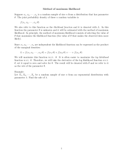
The method of maximum likelihood
4
Large sample hypothesis tests
Reference: Greene, chapter 14 and Appendix D.
EC501 Econometric Methods and Applications
4. Large Sample Methods
Review
3/24
CLRM: y = Xβ + .
The OLS estimator, b = (X 0 X)−1 X 0 y, is BLUE.
Hypothesis tests: t- and F-statistics.
Exact t- and F-distributions rely on assumption of normality.
We shall attempt to see what happens when we relax the
assumption of normality in due course.
To do this we shall use large sample (asymptotic) methods.
EC501 Econometric Methods and Applications
4. Large Sample Methods
Large sample concepts
4/24
If we wish to relax some of the assumptions of the CLRM
then exact finite sample results are typically not available.
For example, if we relax the normality assumption,
t-statistics no longer have t-distributions, F-statistics no
longer have F-distributions etc.
Hence the critical values from these distributions are not
correct, and incorrect inferences may be drawn from the
tests.
We therefore use large sample methods to find out the
properties of estimators and test statistics as n → ∞.
For large enough n we treat the asymptotic results as
holding approximately.
EC501 Econometric Methods and Applications
4. Large Sample Methods
Large sample concepts
5/24
Consider a sequence of numbers indexed by n e.g.
1
1 1 1
−n
,
,
,..., n,... .
{xn = e } =
e e2 e3
e
We can define the limit of this sequence as n → ∞:
lim xn = lim e−n = 0.
n→∞
n→∞
The sequence {xn } is said to converge to zero.
EC501 Econometric Methods and Applications
4. Large Sample Methods
Large sample concepts
6/24
What happens if the elements are random variables?
The sequence of random variables {xn } is said to
converge in probability to a constant c if
lim Pr (|xn − c| > ) = 0 for some > 0.
n→∞
This is written
p
xn → c or plim xn = c.
In words: there exists a positive number such that, as n
gets larger and larger, the probability that the distance
between xn and c is larger than , converges to zero.
EC501 Econometric Methods and Applications
4. Large Sample Methods
Large sample concepts
7/24
If plim b = β then b is a consistent estimator of β.
Consistency is a large sample version of unbiasedness.
A useful property of the plim operator is:
Slutsky’s Theorem
Slutsky’s Theorem: If g(·) is a continuous function and
plim xn = c, then
plim g(xn ) = g(plim xn ) = g(c)
(see D-12 on p.1113 of Greene).
This is not a property shared by the expectations operator
– in general, E[g(x)] 6= g[E(x)] for a random variable x.
EC501 Econometric Methods and Applications
4. Large Sample Methods
Large sample concepts
8/24
Another useful result is:
Chebychev’s Lemma
If xn is a random sequence such that
lim E(xn ) = c and
n→∞
lim var(xn ) = 0,
n→∞
then plim xn = c (see D-1 on p.1107 of Greene).
This enables us to establish consistency by examining the
limiting properties of the expectation and variance.
EC501 Econometric Methods and Applications
4. Large Sample Methods
Large sample concepts
9/24
Convergence to a constant θ is illustrated above by the
variance of the distribution becoming smaller as n
increases.
EC501 Econometric Methods and Applications
4. Large Sample Methods
Large sample concepts
10/24
We are also interested in the distribution of random
variables.
Suppose Fn (·), the distribution function of xn , converges to
a distribution function F(·) as n → ∞.
Then F(·) is the limiting distribution of xn , and if x is a
random variable having distribution function F(·), then xn is
said to converge in distribution to x.
For example, if x ∼ N(0, σ 2 ) and xn converges in
distribution to x, then we write
d
d
xn → x ∼ N(0, σ 2 ) or xn → N(0, σ 2 ).
EC501 Econometric Methods and Applications
4. Large Sample Methods
Large sample concepts
11/24
A useful result concerning convergence in distribution is:
Cramer’s Theorem
If An is a matrix sequence such that plim An = A, and bn is a
d
vector sequence such that bn → b ∼ N(0, Q), then
d
An bn → Ab ∼ N(0, AQA0 ).
This is useful in studying the limiting distribution of the OLS
estimator.
EC501 Econometric Methods and Applications
4. Large Sample Methods
The method of maximum likelihood
12/24
Consider the classical model
yi = xi0 β + i , i = 1, . . . , n; xi nonrandom; i ∼ NID(0, σ 2 ).
(1)
NB: ‘NID(0, σ 2 )’ means ‘normally and independently
distributed with mean zero and variance σ 2 ’.
The normality assumption means the pdf for i is
1
2i
f (i ) = √ exp − 2 , −∞ < i < ∞.
2σ
σ 2π
The independence of the i means the joint pdf for the
n × 1 vector is:
n
Pn 2 n
Y
1
√
f () =
f (i ) =
exp − i=12 i .
2σ
σ 2π
i=1
EC501 Econometric Methods and Applications
4. Large Sample Methods
(2)
(3)
The method of maximum likelihood
13/24
Because y = Xβ + and
obtain the joint pdf for y:
f (y) =
1
2πσ 2
n/2
P
2i = 0 = (y − Xβ)0 (y − Xβ) we
(y − Xβ)0 (y − Xβ)
exp −
2σ 2
.
(4)
This is a function of y for given β and σ 2 .
But in econometrics we need to estimate β and σ 2 for
given y.
The method of maximum likelihood takes the probability
density in (4) and chooses the values of β and σ 2 which
are most likely to have given the observed y.
EC501 Econometric Methods and Applications
4. Large Sample Methods
The method of maximum likelihood
14/24
When regarded as a function of β and σ 2 for given y the
function in (4) is called the likelihood function L(β, σ 2 ; y):
(y − Xβ)0 (y − Xβ)
2
2 −n/2
L(β, σ ; y) = 2πσ
exp −
(5)
2σ 2
We need to maximise (5) with respect to β and σ 2 .
It is easiest to take logs:
n
n
S(β)
ln L = − ln 2π − ln σ 2 −
,
2
2
2σ 2
where S(β) = (y − Xβ)0 (y − Xβ) is the familiar sum of
squares function.
EC501 Econometric Methods and Applications
4. Large Sample Methods
(6)
The method of maximum likelihood
15/24
The first-order conditions for the maximisation are:
∂ ln L
∂β
= −
∂S(β) 1
∂S(βˆML )
· 2 =0 ⇒
= 0;
∂β
2σ
∂β
∂ ln L
∂σ 2
= −
n
S(β)
S(βˆML )
2
+
=
0
⇒
σ
ˆ
=
. (8)
ML
2σ 2
2σ 4
n
(7)
Clearly, from (7), βˆML = b, the OLS estimator:
βˆML = (X 0 X)−1 X 0 y,
2
σ
ˆML
=
(9)
(y − X βˆML )0 (y − X βˆML )
6= s2 .
n
EC501 Econometric Methods and Applications
4. Large Sample Methods
(10)
The method of maximum likelihood
16/24
Consider a general estimation problem where we want to
estimate an m × 1 parameter vector θ whose true value is
θ0 .
Let
g(θ) =
∂ ln L(θ)
(m × 1),
∂θ
H(θ) =
∂ 2 ln L(θ)
(m × m).
∂θ∂θ0
Note that the maximum likelihood estimator (MLE) θˆ
ˆ = 0.
satisfies g(θ)
EC501 Econometric Methods and Applications
4. Large Sample Methods
The method of maximum likelihood
17/24
The MLE θˆ has the following properties:
1
2
3
Consistency: plim θˆ = θ0 .
a
Asymptotic normality: θˆ ∼ N θ0 , I(θ0 )−1 , where
I(θ) = −E[H(θ)] is the information matrix.
Asymptotic efficiency: θˆ achieves the Cramer-Rao lower
bound for consistent estimators, meaning that
ˆ = I(θ0 )−1
var(θ)
˜ var(θ)
˜ ≥ I(θ0 )−1 ).
(in general, for an estimator θ,
Although we have concentrated on the CLRM, maximum
likelihood can be applied in a wide variety of problems,
provided we can write down the density function!
EC501 Econometric Methods and Applications
4. Large Sample Methods
Large sample hypothesis tests
18/24
Sometimes we want to test hypotheses involving
nonlinear restrictions of the form
H0 : c(θ) = 0 against H1 : c(θ) 6= 0
(11)
where θ is an m × 1 vector of parameters and the function
c : Rm → RJ (J ≤ m) i.e. c(θ) is J × 1.
Linear restrictions are a special case: c(θ) = Rθ − q.
Let θˆ be the unrestricted MLE and θˆR be the restricted
MLE:
θˆ = arg max L(θ); θˆR = arg max L(θ) s.t. c(θ) = 0,
θ
θ
where L(θ) is the likelihood function.
There are three large sample tests based on L(θ):
EC501 Econometric Methods and Applications
4. Large Sample Methods
Large sample hypothesis tests
19/24
ˆ
Wald Test: Based on unrestricted estimator θ:
h
i−1
d
ˆ 0 C(θ)I(
ˆ θ)
ˆ −1 C(θ)
ˆ0
ˆ →
W = c(θ)
c(θ)
χ2J
(12)
under H0 as n → ∞, where
C(θ) =
∂c(θ)
(J × m).
∂θ0
and I(θ) denotes the information matrix
2
∂ ln L(θ)
I(θ) = −E
(m × m).
∂θ∂θ0
Easy to use when restrictions are difficult to impose on the
model.
EC501 Econometric Methods and Applications
4. Large Sample Methods
Large sample hypothesis tests
20/24
Likelihood Ratio Test: Based on both θˆ and θˆR .
Let
λ=
L(θˆR )
.
ˆ
L(θ)
Then LR = −2 ln λ i.e.
h
i
d
ˆ − ln L(θˆR ) →
χ2J
LR = 2 ln L(θ)
under H0 as n → ∞.
It can be of interest to compare θˆ and θˆR .
EC501 Econometric Methods and Applications
4. Large Sample Methods
(13)
Large sample hypothesis tests
21/24
Lagrange Multiplier Test: Based on θˆR :
h
i−1
d
LM = g(θˆR )0 I(θˆR )
g(θˆR ) → χ2J
(14)
under H0 as n → ∞, where
g(θ) =
∂ ln L(θ)
.
∂θ
Easy to use when it is difficult to estimate the unrestricted
model.
EC501 Econometric Methods and Applications
4. Large Sample Methods
Large sample hypothesis tests
22/24
The three tests are depicted above.
EC501 Econometric Methods and Applications
4. Large Sample Methods
Large sample hypothesis tests
23/24
Which test should be used, and when?
A key consideration is how easy it is to estimate under H0
and H1 .
The tests are, however, asymptotically equivalent under
the null hypothesis.
But note that different inferences can be drawn from testing
the same hypothesis with the different tests.
In the CLRM, for example, it can be shown that
LM ≤ LR ≤ W.
In such circumstances, if LM rejects H0 , then so will LR and
W, while if W does not reject H0 , then neither will LM or LR.
EC501 Econometric Methods and Applications
4. Large Sample Methods
Summary
24/24
Summary
large sample convergence concepts
maximum likelihood estimation
large sample hypothesis tests
Next week:
OLS in large samples
instrumental variables estimation
EC501 Econometric Methods and Applications
4. Large Sample Methods