1. science
2. mathematics
3. geometry

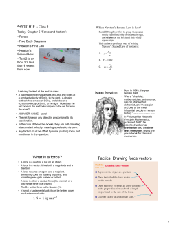
HSC Mathematics Ext. 1 (3 Unit)
SAMPLE LECTURE SLIDES
HSC Exam Preparation Programs
22-26 September, 2014
c 2014 Sci SchoolTM . All rights reserved.
Overview
1. Further
Trigonometry
1. Further Trigonometry
2. Circle Geometry
2. Circle Geometry
3. Parametric
Equations
3. Parametric Equations
4. Mathematical
Induction
4. Mathematical Induction
5. Polynomials
6. Binomial Theorem
7. Further Probability
8. Integration
Methods
9. Inverse
Trigonometric
Functions
10. Rates of Change
11. Rectilinear
Motion
12. Projectile Motion
13. Simple Harmonic
Motion
5. Polynomials
6. Binomial Theorem
7. Further Probability
8. Integration Methods
9. Inverse Trigonometric Functions
10. Rates of Change
11. Rectilinear Motion
12. Projectile Motion
13. Simple Harmonic Motion
© 2014 Sci School
1. Further
Trigonometry
2. Circle Geometry
3. Parametric
Equations
4. Mathematical
Induction
5. Polynomials
6. Binomial Theorem
7. Further Probability
10. Rates of Change
8. Integration
Methods
9. Inverse
Trigonometric
Functions
10. Rates of Change
10.1 Chain Rule
Applications
10.2 Newton’s Law of
Cooling
10.3 HSC-Adapted
Questions
11. Rectilinear
Motion
12. Projectile Motion
13. Simple Harmonic
Motion
© 2014 Sci School
10.1 Chain Rule Applications
1. Further
Trigonometry
2. Circle Geometry
3. Parametric
Equations
4. Mathematical
Induction
5. Polynomials
In the 2 Unit course, we learned that ‘the rate of change’ of a function, Q(t),
means ‘the derivative with respect to time’, i.e. dQ
dt .
In the 3 Unit course, Q may not be explicitly known as a function of t but of
another variable, u, instead. Hence, dQ
dt must be found using the Chain Rule.
6. Binomial Theorem
dQ(u) du
dQ
=
·
dt
du
dt
7. Further Probability
8. Integration
Methods
9. Inverse
Trigonometric
Functions
10. Rates of Change
10.1 Chain Rule
Applications
10.2 Newton’s Law of
Cooling
10.3 HSC-Adapted
Questions
11. Rectilinear
Motion
12. Projectile Motion
13. Simple Harmonic
Motion
•
dQ
Step 1: Write down the known ( du
)
&
unknown
(
dt
dt ) time-derivatives.
•
Step 2: Find the connection between Q and u. We need it explicitly as
Q(u), with no other variables in the expression.
•
Step 3: Differentiate Q(u) to get
dQ
du .
•
Step 4: Substitute your values for
solve for dQ
dt .
dQ
du
and
du
dt
into the Chain Rule to
© 2014 Sci School
10.1 Chain Rule Applications
1. Further
Trigonometry
2. Circle Geometry
3. Parametric
Equations
4. Mathematical
Induction
For example, an inverted cone of base radius 6 cm and height 20 cm has
water flowing from its apex at the constant rate of 6 cm3 /s.
Use the Chain Rule to determine the rate at which the water level is falling
when the water level is 4 cm.
5. Polynomials
6
6. Binomial Theorem
7. Further Probability
8. Integration
Methods
r
9. Inverse
Trigonometric
Functions
20
h
10. Rates of Change
10.1 Chain Rule
Applications
10.2 Newton’s Law of
Cooling
10.3 HSC-Adapted
Questions
11. Rectilinear
Motion
•
Step 1: We want
dh
dt
when h is 4 cm. We know
dV
dt
is −6 cm3 /s.
12. Projectile Motion
13. Simple Harmonic
Motion
© 2014 Sci School
10.1 Chain Rule Applications
1. Further
Trigonometry
•
Step 2: For a cone, V and h are related by V = 13 πr 2 h.
2. Circle Geometry
3. Parametric
Equations
4. Mathematical
Induction
5. Polynomials
6. Binomial Theorem
7. Further Probability
8. Integration
Methods
9. Inverse
Trigonometric
Functions
10. Rates of Change
Since r is also a variable, we need to rearrange the expression so it
contains only V and h as variables. Notice the geometric relationship
between r and h in the diagram: equiangular similar triangles means the
h
ratio r6 is equal to 20
.
Hence,
h
r =6×
20
Substituting this into our volume expression gives,
10.1 Chain Rule
Applications
10.2 Newton’s Law of
Cooling
10.3 HSC-Adapted
Questions
11. Rectilinear
Motion
12. Projectile Motion
13. Simple Harmonic
Motion
=⇒
3h
r=
10
3h
1
π
3
10
3π 3
h
∴ V =
100
V =
2
h
© 2014 Sci School
10.1 Chain Rule Applications
1. Further
Trigonometry
•
Step 3: Differentiating V =
3π 3
100 h
gives us,
2. Circle Geometry
dV
9π 2
=
h
dh
100
3. Parametric
Equations
4. Mathematical
Induction
5. Polynomials
6. Binomial Theorem
7. Further Probability
8. Integration
Methods
9. Inverse
Trigonometric
Functions
•
Step 4: Substituting our values for
or
dh
dV
100
dh
=
dV
9πh2
and
dV
dt
into the Chain Rule,
dh
dh dV
=
·
dt
dV dt
100
dh
3
=
· −6 cm /s
∴
dt
9πh2
10. Rates of Change
10.1 Chain Rule
Applications
10.2 Newton’s Law of
Cooling
10.3 HSC-Adapted
Questions
11. Rectilinear
Motion
12. Projectile Motion
13. Simple Harmonic
Motion
Lastly, at a water level of 4 cm, our expression simplifies to
200 cm3 /s
dh
=−
2
dt
3π (4 cm)
25
dh
=
−
cm/s
∴
dt
6π
when h = 4 cm
© 2014 Sci School
10.2 Newton’s Law of Cooling
1. Further
Trigonometry
2. Circle Geometry
3. Parametric
Equations
4. Mathematical
Induction
5. Polynomials
6. Binomial Theorem
7. Further Probability
8. Integration
Methods
9. Inverse
Trigonometric
Functions
10. Rates of Change
10.1 Chain Rule
Applications
10.2 Newton’s Law of
Cooling
10.3 HSC-Adapted
Questions
11. Rectilinear
Motion
This is an extension on Exponential Growth and Decay discussed in the 2
Unit course.
Newton showed that an object’s temperature is governed by,
dT
= −k(T − Tf )
dt
where k > 0 is a constant and Tf is the equilibration (final) temperature.
The solution to this equation is found by integrating the inverse expression.
That is, we first invert Newton’s differential equation,
dt
−1
=
.
dT
k(T − Tf )
12. Projectile Motion
13. Simple Harmonic
Motion
© 2014 Sci School
10.2 Newton’s Law of Cooling
1. Further
Trigonometry
2. Circle Geometry
3. Parametric
Equations
4. Mathematical
Induction
5. Polynomials
Secondly, we integrate the fraction to form a log,
−1
dT
t=
k(T − Tf )
−1
=
ln(T − Tf ) + C.
k
6. Binomial Theorem
7. Further Probability
8. Integration
Methods
9. Inverse
Trigonometric
Functions
10. Rates of Change
10.1 Chain Rule
Applications
10.2 Newton’s Law of
Cooling
10.3 HSC-Adapted
Questions
11. Rectilinear
Motion
12. Projectile Motion
13. Simple Harmonic
Motion
Subtracting C and multiplying by −k, give us,
−kt + kC = ln(T − Tf ).
We can now exponentiate both sides to arrive at
e−kt+kC = T − Tf
or Ae−kt = T − Tf ,
if we define a simplified constant as A = ekC . Solving for T gives us,
T (t) = Tf + Ae−kt
© 2014 Sci School
10.2 Newton’s Law of Cooling
1. Further
Trigonometry
2. Circle Geometry
3. Parametric
Equations
4. Mathematical
Induction
5. Polynomials
6. Binomial Theorem
The constant A represents the difference between initial and final
temperatures. To see this, substitute t = 0 into T (t) to arrive at
T (0) = Tf + A, or A = T0 − Tf .
T (t)
T0
T (t) = Tf + Ae−kt
7. Further Probability
8. Integration
Methods
9. Inverse
Trigonometric
Functions
10. Rates of Change
A>0
Tf
10.1 Chain Rule
Applications
A<0
10.2 Newton’s Law of
Cooling
10.3 HSC-Adapted
Questions
11. Rectilinear
Motion
T0
t
12. Projectile Motion
13. Simple Harmonic
Motion
© 2014 Sci School
10.2 Newton’s Law of Cooling
1. Further
Trigonometry
2. Circle Geometry
3. Parametric
Equations
4. Mathematical
Induction
5. Polynomials
6. Binomial Theorem
For example, given a cooling constant of 0.06 min−1 , how much quicker is it
to chill 18◦ C tap water to 7◦ C when using a 5◦ C refrigerator compared with a
-20◦ C freezer?
•
Refrigerator data: T (t) = 7◦ C, T0 = 18◦ C, Tf = 5◦ C ∴ A = 13◦ C.
•
Step 1: Substitute the data into Newton’s temperature formula.
7 = 5 + 13e−0.06t
2
= e−0.06t
∴
13
7. Further Probability
8. Integration
Methods
9. Inverse
Trigonometric
Functions
10. Rates of Change
10.1 Chain Rule
Applications
10.2 Newton’s Law of
Cooling
10.3 HSC-Adapted
Questions
11. Rectilinear
Motion
12. Projectile Motion
13. Simple Harmonic
Motion
•
Step 2: Solve for t by taking logs of both sides,
2
= −0.06t
ln
13
2
1
ln
= 31.2 min
∴ t=−
0.06
13
© 2014 Sci School
10.2 Newton’s Law of Cooling
1. Further
Trigonometry
•
Freezer data: T (t) = 7◦ C, T0 = 18◦ C, Tf = −20◦ C ∴ A = 38◦ C.
2. Circle Geometry
•
Step 1: Substitute the data into Newton’s temperature formula.
3. Parametric
Equations
7 = −20 + 38e−0.06t
27
= e−0.06t
∴
38
4. Mathematical
Induction
5. Polynomials
6. Binomial Theorem
7. Further Probability
8. Integration
Methods
9. Inverse
Trigonometric
Functions
10. Rates of Change
10.1 Chain Rule
Applications
10.2 Newton’s Law of
Cooling
10.3 HSC-Adapted
Questions
11. Rectilinear
Motion
•
Step 2: Solve for t by taking logs of both sides,
27
= −0.06t
ln
38
27
1
ln
= 5.7 min
∴ t=−
0.06
38
Hence, the freezer is 26 minutes faster than the refrigerator at chilling the
water from 18◦ C to 7◦ C.
12. Projectile Motion
13. Simple Harmonic
Motion
© 2014 Sci School
10.3 HSC-Adapted Questions
1. Further
Trigonometry
Quesiton 1 (4 Marks)
2. Circle Geometry
Alice, Bob, and Charlie stand so as to form a right-angled triangle, with
Charlie and Bob forming the hypotenuse and Alice and Bob separated by
20 metres. Charlie proceeds to walk towards Alice at a constant rate of
change of 2 metres per second. At what rate is the distance between Charlie
and Bob changing, when Charlie is 15 metres from Alice?
3. Parametric
Equations
4. Mathematical
Induction
5. Polynomials
6. Binomial Theorem
7. Further Probability
8. Integration
Methods
9. Inverse
Trigonometric
Functions
Solution
10.1 Chain Rule
Applications
Let the distances between Charlie and Alice and Charlie and Bob be a and b,
da
respectively. We need to calculate db
dt when a is 15 metres. We know that dt
is −2 metres per second, since the distance is decreasing.
10.2 Newton’s Law of
Cooling
Using Pythagorus’ Theorem,
10. Rates of Change
10.3 HSC-Adapted
Questions
11. Rectilinear
Motion
12. Projectile Motion
13. Simple Harmonic
Motion
202 + a2 = b2
∴ b = 400 + a2
© 2014 Sci School
10.3 HSC-Adapted Questions
1. Further
Trigonometry
2. Circle Geometry
3. Parametric
Equations
4. Mathematical
Induction
5. Polynomials
6. Binomial Theorem
7. Further Probability
8. Integration
Methods
9. Inverse
Trigonometric
Functions
10. Rates of Change
10.1 Chain Rule
Applications
10.2 Newton’s Law of
Cooling
10.3 HSC-Adapted
Questions
11. Rectilinear
Motion
12. Projectile Motion
13. Simple Harmonic
Motion
Differentiating this expression, we have
1
d db
2 2
=
400 + a
da
da
1
1 2 −2
= × 400 + a
× 2a
2
a
= √
400 + a2
3
= , when a = 15
5
Substituting these values into the Chain Rule, we arrive at
db
3
= × −2
dt
5
6
=−
5
Hence, when Charlie is 15 m from Alice, he approaches Bob at 1.2 m/s.
© 2014 Sci School
10.3 HSC-Adapted Questions
1. Further
Trigonometry
Quesiton 2 (3 Marks)
2. Circle Geometry
A cup of tea has an initial temperature of 100◦ C. The temperature, T ◦ C, of
the tea after t minutes is given by
3. Parametric
Equations
4. Mathematical
Induction
T (t) = X + Y e−kt ,
5. Polynomials
6. Binomial Theorem
7. Further Probability
8. Integration
Methods
9. Inverse
Trigonometric
Functions
10. Rates of Change
10.1 Chain Rule
Applications
10.2 Newton’s Law of
Cooling
10.3 HSC-Adapted
Questions
where X, Y , and k are positive constants.
In a room with an ambient temperature of 19◦ C, the temperature of the tea
drops to 85◦ C after 5 minutes. How long does the tea take to cool to 50◦ C?
Solution
The final temperature of the tea will be 19◦ C, ∴ X = 19◦ C.
Also, we are told that T (0) = 100◦ C, ∴ Y = (100 − 19)◦ C = 81◦ C.
11. Rectilinear
Motion
12. Projectile Motion
13. Simple Harmonic
Motion
© 2014 Sci School
10.3 HSC-Adapted Questions
1. Further
Trigonometry
2. Circle Geometry
3. Parametric
Equations
4. Mathematical
Induction
5. Polynomials
6. Binomial Theorem
7. Further Probability
8. Integration
Methods
9. Inverse
Trigonometric
Functions
10. Rates of Change
10.1 Chain Rule
Applications
10.2 Newton’s Law of
Cooling
10.3 HSC-Adapted
Questions
11. Rectilinear
Motion
12. Projectile Motion
13. Simple Harmonic
Motion
When t = 5, T = 85◦ C. Substituting this into the equation, we have
80 = 19 + 81e−k×5
61 = 81e−5k
61
= e−5k
81
61
1
∴ k = − ln
5
81
Now that all the constants are known, we can substitute T = 50◦ C.
1
5
ln( 61
81 )t
50 = 19 + 81e
1
61
31
= e 5 ln( 81 )t
81
31 ln 81
∴ t = 1 61 = 16.9 minutes
5 ln 81
© 2014 Sci School
10.3 HSC-Adapted Questions
1. Further
Trigonometry
Quesiton 3 (6 Marks)
2. Circle Geometry
At 3pm in a school playground, a melted chocolate bar is found to be at a
temperature of x◦ C. The packaging on the chocolate bar says it will begin to
melt at 16◦ C. The temperature, T ◦ C, of the bar t minutes after 3pm varies
according to the differential equation
3. Parametric
Equations
4. Mathematical
Induction
5. Polynomials
6. Binomial Theorem
dT
1
=
ln(1.6)(A − T ),
dt
60
7. Further Probability
8. Integration
Methods
9. Inverse
Trigonometric
Functions
10. Rates of Change
10.1 Chain Rule
Applications
10.2 Newton’s Law of
Cooling
10.3 HSC-Adapted
Questions
11. Rectilinear
Motion
12. Projectile Motion
13. Simple Harmonic
Motion
where A is a constant.
(i) Show that for any constant, B, a solution to the differential equation is
T = A + Be
1
− 60
ln(1.6)t
.
◦
(ii) After an hour, the chocolate bar increases in temperature by 15
4 C. Given
the chocolate bar started to melt at 2pm, find x and the limiting temperature
of the bar. Assume the temperature of the day is constant.
© 2014 Sci School
10.3 HSC-Adapted Questions
1. Further
Trigonometry
Solution
2. Circle Geometry
(i) Differentiating the proposed solution, we have
3. Parametric
Equations
1
d dT
=
A + Be− 60 ln(1.6)t
dt
dt
1
1
− 60
ln(1.6)t
= Be
× − ln (1.6)
60
1
= (T − A) × − ln (1.6)
60
1
ln(1.6)(A − T )
=
60
4. Mathematical
Induction
5. Polynomials
6. Binomial Theorem
7. Further Probability
8. Integration
Methods
9. Inverse
Trigonometric
Functions
10. Rates of Change
10.1 Chain Rule
Applications
10.2 Newton’s Law of
Cooling
10.3 HSC-Adapted
Questions
as required.
(ii) We are told that T (0) = x◦ C, ∴ x = A + B.
11. Rectilinear
Motion
12. Projectile Motion
13. Simple Harmonic
Motion
© 2014 Sci School
10.3 HSC-Adapted Questions
1. Further
Trigonometry
When t = −60, T = 16◦ C. Substituting these values into the equation,
2. Circle Geometry
3. Parametric
Equations
4. Mathematical
Induction
5. Polynomials
6. Binomial Theorem
7. Further Probability
8. Integration
Methods
9. Inverse
Trigonometric
Functions
10. Rates of Change
10.1 Chain Rule
Applications
10.2 Newton’s Law of
Cooling
10.3 HSC-Adapted
Questions
11. Rectilinear
Motion
12. Projectile Motion
13. Simple Harmonic
Motion
16 = A + Be
1
− 60
ln(1.6)×−60
16 = A + Beln(1.6)
16 = A + B × 1.6
16 − A
∴ B=
1.6
When t = 60, T = (x +
15 ◦
4 ) C.
Hence, we have
15
4
15
A+B+
4
15
B+
4
∴ B
x+
1
= A + Be− 60 ln(1.6)×60
= A + Be
=B×
= −10
− ln( 16
10 )
10
16
© 2014 Sci School
10.3 HSC-Adapted Questions
1. Further
Trigonometry
Combining these equations, we have
16 − A
= −10
1.6
∴ A = 16 + 16 = 32
2. Circle Geometry
3. Parametric
Equations
4. Mathematical
Induction
5. Polynomials
6. Binomial Theorem
7. Further Probability
8. Integration
Methods
9. Inverse
Trigonometric
Functions
10. Rates of Change
10.1 Chain Rule
Applications
10.2 Newton’s Law of
Cooling
10.3 HSC-Adapted
Questions
11. Rectilinear
Motion
12. Projectile Motion
13. Simple Harmonic
Motion
Since x = A + B, we have
x = 32 − 10
∴ x = 22
1
The limiting temperature occurs when t → ∞. Since e− 60 ln(1.6)t → 0 as
t → ∞, we arrive at
T (t → ∞) = 32 − 10 × 0
= 32
which is the equilibrium temperature.
© 2014 Sci School