Two-Sample Test for Mean – Vars. Known TMS-061: Lecture 6 Two-sample Tests Settings: X1 is an i. i. d. sample of size n1 from N (µ1 , σ12 ) and X2 is an i. i. d. sample of size n2 from N (µ2 , σ22 ). Variances σ1 , σ2 are known. To test: Sergei Zuyev (i) H0 = {µ1 − µ2 = D} vs. HA = {µ1 − µ2 6= D} or (ii) H0 = {µ1 − µ2 = D} vs. HA = {µ1 − µ2 > D} or (iii) H0 = {µ1 − µ2 = D} vs. HA = {µ1 − µ2 < D} Sergei Zuyev TMS-061: Lecture 6 Two-sample Tests Test Statistic Sergei Zuyev TMS-061: Lecture 6 Two-sample Tests Independent Normal Samples – Vars Unknown σ2 σ2 Since X 1 − X 2 ∼ N µ1 − µ2 , n11 + n22 then an appropriate test statistic is X1 − X2 − D Z = q 2 . σ1 σ22 + n1 n2 Then if H0 holds, Z ∼ N (0, 1). This is two-sample Z-test. It is also applicable for non-normal obs. if n1 , n2 are large (at least 30) The settings, H0 , HA are as for two-sample Z -test, but σ’s are unknown. Replacing them with their estimates – sample variances S1 , S2 , leads to statistic t(ν) = X1 − X2 − D q 2 . S1 S22 n1 + n2 which has t(ν) distr. under H0 . Expression for ν is complicated: (1 − c)2 c2 ν= + n1 − 1 n2 − 1 −1 and c = S12 /n1 . S12 /n1 + S22 /n2 This is Aspin-Welch test. Sergei Zuyev TMS-061: Lecture 6 Two-sample Tests Sergei Zuyev TMS-061: Lecture 6 Two-sample Tests CI for Difference in Means 100%(1 − α)-confidence interval for (µ1 − µ2 ) is s σ12 σ22 X 1 − X 2 ± Zα/2 + n1 n2 Variances are rarely known in practice, so t-test should be more widely used, but ν is messy to compute (by hand). If it is not an integer, as approximation choose the largest integer below ν (does not apply to statistical software) in Z -test and For n1 , n2 big enough (≥ 30) by the CLT we could use Z -test with σ1 , σ2 replaced by the corresponding sample estimates S1 , S2 even for not normal samples. s X 1 − X 2 ± tα/2 (ν) S12 S22 + n1 n2 Most common case is: H0 = {µ1 = µ2 }, i. e. D = 0. in t-test. Sergei Zuyev TMS-061: Lecture 6 Two-sample Tests Sergei Zuyev TMS-061: Lecture 6 Two-sample Tests Equal Variances It is a special case of the above test where we do know that σ1 = σ2 but do not know their common value, say σ. Procedure is to ‘pool’ the samples together to estimate σ as S2 = (n1 − 1)S12 + (n2 − 1)S22 n1 + n2 − 2 100%(1 − α)-confidence interval for (µ1 − µ2 ) is p X 1 − X 2 ± tα/2 (n1 + n2 − 2) S 1/n1 + 1/n2 . The test assumes a lot: normality, independence, equality of vars. If no reason to believe σ1 = σ2 , use Aspin-Welch test. Test-statistic: t= X1 − X2 − D p ∼ t(n1 + n2 − 2) S 1/n1 + 1/n2 called two-sample t-test. Sergei Zuyev TMS-061: Lecture 6 Two-sample Tests Sergei Zuyev TMS-061: Lecture 6 Two-sample Tests Proportions: Two Independent Samples We have two samples of size ni from two populations (i = 1, 2). Yi – No. successes in i-th sample, sample proportions bi = Yi /ni . The true proportionsare pi . p i) bi ∼ N pi , pi (1−p and so For n1 , n2 ≥ 50 we have p ni p (1 − p1 ) p2 (1 − p2 ) b1 − p b2 ≈ N p1 − p2 , 1 p + n1 n2 Hence, test statistic for H0 = {p1 − p2 = D} is Z =q b1 − p b2 − D p b p1 (1−b p1 ) n1 + b p2 (1−b p2 ) n2 , 100%(1 − α)-confidence interval for (p1 − p2 ) is s b1 (1 − p b1 ) p b2 (1 − p b2 ) p b1 − p b2 ± Zα/2 p + n1 n2 Commonest case is D = 0, i. e. H0 = {p1 = p2 } = p, say. Then we can pool the samples to estimate the common p: b= p b1 − p b2 Y1 + Y2 p and Z = p n1 + n2 b(1 − p b)(1/n1 + 1/n2 ) p which is approx. N (0, 1). which has approx. N (0, 1) distribution if H0 is true. Sergei Zuyev TMS-061: Lecture 6 Two-sample Tests Sergei Zuyev TMS-061: Lecture 6 Two-sample Tests Test of Variances Equality of variances is an important assumption of two-sample tests above, and we can actually test this assumption statistically. Setting: two independent normal samples of sizes n1 , n2 . To test: H0 = {σ1 = σ2 } against HA = {σ1 6= σ2 } (or HA = {σ1 > σ2 } or HA = {σ1 < σ2 }). Test statistics: F = S12 /S22 ∼ F (n1 − 1, n2 − 1) if H0 true If test is one-sided – use upper tail only: If HA = {σ1 > σ2 } compute F = S12 /S22 If HA = {σ1 < σ2 } compute F = S22 /S12 F -test is two-sided (as when we want to confirm assumptions of t-test) then we still use only upper α/2-tails but compute the ratio so that F > 1: if S1 > S2 , F = S12 /S22 , if S1 < S2 then F = S22 /S12 . has Fisher–Snedecor F -distribution with n1 − 1 and n2 − 1 degrees of freedom (both parameters are called degrees of freedom). 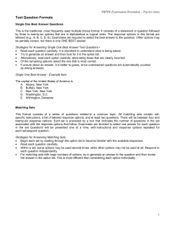Sergei Zuyev TMS-061: Lecture 6 Two-sample Tests Sergei Zuyev TMS-061: Lecture 6 Two-sample Tests F -distribution Tables give upper-tail quantiles only. Tables are not symmetric as the first degree is associated with numerator, while the second – with denominator. If lower tails really needed, e. g. for CI’s, use result: Fα (ν1 , ν2 ) = F0.05 (4, 7) = 4.12 1 F1−α (ν2 , ν1 ) α = 0.05 If lower tails really needed, e. g. for CI’s, use result: Sergei Zuyev TMS-061: Lecture 6 Two-sample Tests 1 Fα (ν1 , ν2 ) = F1−α (ν2 , ν1 ) Related Normal Samples 0.3 TMS-061: Lecture 6 Two-sample Tests Summary statistics: Example: Five subjects given analgesic A gained additional sleep per night (hours) averaged over 10 nights from the long-term pre-treatment mean as follows: 2.1 Sergei Zuyev −1.6 4.0 1.5 x¯A = 1.26 sA2 = 4.343 nA = 5 x¯B = 2.14 sB2 = 4.465 nB = 5. Carrying out the (pooled variance) 2-sample t-test of against H0 : µA = µB H1 : µA = 6 µB Five subjects given analgesic B reported gains as follows: 3.2 0.5 0.0 5.2 1.8 Assuming hours gained are normally distributed with the same variance in both groups, is there evidence that either of the analgesics is more effective than the other in increasing sleep per night? Sergei Zuyev TMS-061: Lecture 6 Two-sample Tests 4sA2 + 4sB2 = 4.4055; 8 x¯A − x¯B t=p = −0.66; 2 s (1/nA + 1/nB ) s2 = However from the table of the t-distribution t8,0.025 = 2.306 and so this is not significant at the 5% significance level. There is no good reason to believe there is any difference between A nad B. Sergei Zuyev TMS-061: Lecture 6 Two-sample Tests However, let us now suppose these data were collected in a cross-over trial, and that the samples are not independent, but instead that corresponding figures refer to the same subject. Subject 1 2 3 4 5 A 2.1 0.3 -1.6 4.0 1.5 Sergei Zuyev D = 0.88 B 3.2 0.5 0.0 5.2 1.8 D =B−A 1.1 0.2 1.6 1.2 0.3 TMS-061: Lecture 6 Two-sample Tests sD2 = 0.367 n = 5; D−0 = 3.25. t=q sD2 /n From the table t4,0.025 = 2.776, so this result is significant, and there is quite strong evidence that B is more effective than A (since evidently µD > 0). N.B. It is only if data have been collected so that corresponding values come from matched sources that this analysis of differences is possible. It is not applicable if the comparison data come from independent samples. Sergei Zuyev TMS-061: Lecture 6 Two-sample Tests The differences D will also be normally distributed, and so we may test against H0 : µD = 0 H1 : µD = 6 0 with a 1-sample t-test. Sergei Zuyev TMS-061: Lecture 6 Two-sample Tests