Flexible Sample Size Considerations Using Information
Based Interim Monitoring
Cyrus R. Mehta
Cytel Software Corporation
and
Anastasios A. Tsiatis
North Carolina State University
19 March 2001
Abstract
At the design phase of a clinical trial the total number of participants needed to
detect a clinically important treatment diﬀerence with suﬃcient precision depends
frequently on nuisance parameters like variance, baseline response rate, or regression
coeﬃcients other than the main eﬀect. In practical applications, nuisance parameter
values are often unreliable guesses founded on little or no available past history. Sample
size calculations based on these initial guesses may therefore lead to over or
underpowered studies. In this paper we argue that the precision with which a treatment
eﬀect is estimated is, directly related to the statistical information in the data. In
general, statistical information is a complicated function of sample size and nuisance
parameters. However, the amount of information necessary to answer the scientiﬁc
question concerning treatment diﬀerence is easily calculated a priori and applies to
almost any statistical model for a large variety of endpoints. It is thus possible to be
ﬂexible on sample size but rather continue collecting data until we have achieved the
desired information. Such a strategy is well suited to being adopted in conjunction with a
group sequential clinical trial where the data are monitored routinely anyway. We
present several scenarios and examples of how group sequential information-based design
and monitoring can be carried out and demonstrate through simulations that this type of
strategy will indeed give us the desired operating characteristics.
1
1
Introduction
At the design phase of a randomized clinical trial the total number of participants needed to
achieve a certain level of signiﬁcance and power depends frequently on nuisance parameters
like variance, baseline response rate, or regression coeﬃcients other than the main eﬀect. In
practical applications, nuisance parameter values are often unreliable guesses founded on little
or no available past history. As a result, if the initial guesses for the nuisance parameters are
far from the truth, then the study may be under or over powered to detect the desired
treatment diﬀerence.
For example, in a clinical trial comparing dichotomous responses, suppose the investigators
want to design the study to detect a 10% diﬀerence in the response rate between a new
treatment and a control treatment with 90% power using a test at the 0.05 (two-sided) level of
signiﬁcance. The traditional approach would necessitate that an initial guess be made for the
response rate in the control group. Say this is given to be 20%, using the best available data.
It is then a simple exercise to show that a total of 778 participants, randomized with equal
probability to the two treatments, would provide the required 90% power for a two-sided level
0.05 test to detect a diﬀerence from 20% to 30%. In truth, however, suppose the initial guess
was wrong and the response rate for the control group was 40%. Then with a sample size of
778, the power of the binomial test at the .05 level of signiﬁcance to detect a 10% diﬀerence, or
a diﬀerence from 40% to 50%, would have been diminished to 80%. To achieve 90% power one
would need 1030 participants.
For ethical as well as practical considerations most large Phase III randomized clinical trials
are designed with formal sequential stopping rules. The data from such a clinical trial are
monitored at interim time-points, usually by an external data and safety monitoring board,
and if the observed treatment diﬀerence is suﬃciently large at one of these interim analyses,
the study may be stopped. Formal sequential boundaries have been derived that dictate how
large the treatment diﬀerence must be at diﬀerent interim analyses before a study is stopped.
These boundaries are constructed so that the overall test has the desired operating
characteristics. That is, the resulting sequential test will have the desired level of signiﬁcance
and power to detect a clinically important treatment diﬀerence. Issues regarding the eﬀect on
power of misspecifying the nuisance parameter during the design stage are similar to those
discussed earlier for the ﬁxed sample procedure. However, when data are monitored
periodically, the nuisance parameters in the model can be estimated with the available data
and, if these estimates are suﬃciently far from the values used at the design stage, the
investigators have the ability to alter the design; i.e., to increase or decease the sample size
adaptively. It is the feasibility of this strategy that we will investigate in this paper.
2
Information Based Design and Interim Monitoring
In this section we will develop a single uniﬁed nuisance-parameter-free information-based
approach for designing and monitoring clinical trials. This approach is applicable to studies
involving dichotomous response, continuous response, time to event response and longitudinal
2
response, in the presence of one or more nuisance parameters, including covariates. In all these
settings we assume that the data are generated from some multiparameter probability model
in which a single unknown parameter, δ, characterizes the beneﬁt conferred by the new
treatment under investigation while the remaining unknown parameters are denoted as
nuisance parameters whose values play no role in determining the clinical importance of the
new treatment, but are important in properly describing the probability distribution that
generates the data. Interest focuses on testing the null hypothesis
H0 : δ = 0
(2.1)
at the α level of signiﬁcance. Suppose a two-sided test is to be conducted and is required to
have power equal to 1 − β against the alternative hypothesis
Ha : δ = δa .
2.1
(2.2)
Designing Fixed Information Studies
A typical way to carry out a two-sided ﬁxed-information test of the null hypothesis (2.1) is to
ﬁt the underlying model to all the data available at the end of the study, compute the Wald
test statistic
δˆ
T =
,
(2.3)
ˆ
se(δ)
and reject H0 if
|T | ≥ zα/2 ,
(2.4)
ˆ is an estimate
where zu is the (1 − u)th quantile of the standard normal distribution and se(δ)
ˆ A crucial question to ask is, how much data should we collect before
of the standard error of δ.
we perform the hypothesis test (2.4)? In other words, how much “information” should we
gather? The term information (or Fisher information) has a strict technical meaning which is
ˆ As one might expect intuitively, the smaller the variance, the
related to the variance of δ.
more the information. Now the true variance of δˆ is usually not known. For all practical
purposes, however, the Fisher information available at the end the study can be well
ˆ or [se(δ)]
ˆ −2 . Throughout this
approximated by the inverse of the estimated variance of δ,
development we shall use this approximation as though it were the actual Fisher information.
The amount of Fisher information, I, needed in order for the test (2.4)) to achieve a power of
1 − β can be derived by standard statistical methods as
zα/2 + zβ
I=
δa
where I is approximated by
2
ˆ −2 .
I ≈ [se(δ)]
(2.5)
(2.6)
Thus, operationally, in a ﬁxed information study one would gather data until the inverse
square of the standard error of the estimate of δ equaled the right hand side of equation (2.5),
and would then perform the hypothesis test (2.4).
3
Example 1: Normal Response with Unknown Variance.
Let XA be the response of a subject who receives treatment A and XB be the response of a
subject who receives treatment B. Let µA and µB be the expected values of the random
variables XA and XB , respectively, both normally distributed with a common unknown
variance σ 2 . We are interested in testing the null hypothesis (2.1) in which
δ = µ A − µB .
(2.7)
In a ﬁxed information study we do not ﬁx the sample size in advance. Rather we continue to
enroll subjects into the clinical trial until we have gathered a suﬃcient number, say nA on
treatment A and nB on treatment B, so as to satisfy the ﬁxed information requirement
ˆ
[se(δ)]
−2
σ
ˆ2
σ
ˆ2
≡
+
nA nB
−1
≥
zα/2 + zβ
δa
2
.
(2.8)
¯B .
¯A − X
We then perform the hypothesis test (2.4) using the test statistic (2.3) in which δˆ = X
As long as (2.8) is satisﬁed, the study will have the desired 1 − β power regardless of the true
value of the nuisance parameter σ 2 .
Example 2: Dichotomous Response with Unknown Baseline Probability.
Let πA and πB be the response probabilities for treatment A and B, respectively. We are
interested in testing the null hypothesis (2.1) in which
δ = π A − πB ,
(2.9)
and the baseline response probability πB is unknown. In a ﬁxed information study we enroll
subjects into the clinical trial until the sample size, say nA on treatment A and nB on
treatment B, is large enough to satisfy
ˆ
[se(δ)]
−2
π
ˆA (1 − π
ˆA ) π
ˆB )
ˆB (1 − π
≡
+
nA
nB
−1
≥
zα/2 + zβ
δa
2
.
(2.10)
We then perform the hypothesis test (2.4) using the test statistic (2.3) in which δˆ = π
ˆA − π
ˆB .
With this approach the study will have the desired 1 − β power regardless of the true value of
the nuisance parameter πB .
Example 3: Time to Event Response from Proportional Hazards Model.
Suppose the data are generated from the Cox proportional hazards model
λ(t|Z0 , Z 1 ) = λ0 (t)eδZ0 +ηZ 1 .
(2.11)
We are interested in testing the null hypothesis that δ = 0 in the presence of possibly several
nuisance parameters η. In a ﬁxed information study we enroll subjects into the clinical trial
and follow them until we have satisﬁed the condition
ˆ −2 ≥
[se(δ)]
zα/2 + zβ
δa
2
,
(2.12)
ˆ is its standard error. Once
where δˆ is the maximum partial likelihood estimate of δ, and se(δ)
we have gathered suﬃcient information, as evidenced by satisfying (2.12), we perform the
4
hypothesis test (2.4). With this approach the study will have the desired 1 − β power
regardless of the true values of the nuisance parameters η. Note that many combinations of
subject accrual and follow-up time will satisfy (2.12). For details concerning the trade-oﬀ
between additional accrual and additional follow-up time, refer to Kim and Tsiatis (1990), and
Scharfstein and Tsiatis (1998).
Example 4: Longitudinal Response from Random Eﬀects Model.
Suppose the data are generated from the random eﬀects model
Yijk = αik + γik tijk + ijk ,
where
and
αik
γik
∼N
Ak
Gk
,
σA2 k
σAk ,Gk
σAk ,Gk
2
σG
k
(2.13)
ijk ∼ N (0, σ2k ) ,
k = 1, 2, j = 1, . . . , nik , i = 1, . . . , mk .
We are interested in testing the null hypothesis
H0 : δ = G 1 = G 2 = 0
in the presence of possibly unknown variance components. In a ﬁxed information study we
enroll subjects into the clinical trial and gather longitudinal information on them until we have
satisﬁed the condition
2
ˆ −2 ≥ zα/2 + zβ
[se(δ)]
,
(2.14)
δa
ˆ is its standard error. Once we have
where δˆ is the maximum likelihood estimate of δ, and se(δ)
gathered suﬃcient information, as evidenced by satisfying (2.14), we perform the hypothesis
test (2.4). With this approach the study will have the desired 1 − β power regardless of the
true values of the nuisance parameters η. Note that many combinations of subject accrual and
number of longitudinal observations per subject will satisfy (2.14). For a detailed
implementation of this rather complex design refer to Scharfstein and Tsiatis and Robins
(1997).
2.2
Designing Maximum Information Studies within the Group
Sequential Framework
The ﬁxed information strategy outlined in the previous section has two limitations:
- Unless the accruing data are monitored at interim time-points one has no means of
determining if the desired information has been attained.
- Since information is an abstract quantity, knowing how much information to gather over
the course of a study is not of much practical use in planning the study. For planning
purposes one needs to translate the desired information into a physical resource like
sample size. For this purpose one must use some initial estimates or guesses of the
nuisance parameters.
5
Group sequential designs provide a natural way to overcome both limitations. In a group
sequential study one is already intending to monitor the accruing data at administratively
convenient interim monitoring time-points, with a view to early stopping if a stopping
boundary is crossed. One can therefore take advantage of the interim looks to compute the
current information as well as to update prior estimates of nuisance parameters with the help
of the latest available data.
Suppose that instead of performing only one signiﬁcance test at the end of the study we decide
to perform up to K repeated signiﬁcance tests at interim monitoring times τ1 , τ2 , . . . τK ,
respectively, and to terminate the study at the ﬁrst test that rejects the null hypothesis. The
ﬂexibility to monitor the data in this fashion and possibly terminate the study early comes at
cost.
1. Repeated application of the same signiﬁcance test (2.4) will result in an elevated type-1
error. In order to maintain the type-1 error at level α, the criterion for rejecting the null
hypothesis must be made more stringent. Therefore, if we intend to monitor the trial K
times, the strategy would be to stop the trial and reject the null hypothesis at the ﬁrst
time-point τj , j ≤ K, for which the corresponding test statistic |Tj |, calculated using all
the available data up to time τj , exceeds the stopping boundary cj , where cj must exceed
zα/2 . If the stopping boundary is not crossed at any of the K time-points, then the study
is terminated at the Kth and ﬁnal analysis.
2. The maximum information to be committed up-front in order to achieve a power of 1 − β
gets inﬂated. We must now commit to keeping the study open until the total information
equals
zα/2 + zβ 2
Imax =
× IF(∆, α, β, K)
(2.15)
δa
where IF(.) is an inﬂation factor that depends on α, β, K and ∆, a “shape parameter”
to be deﬁned shortly that determines the shape of the stopping boundary over the K
repeated signiﬁcance tests. We must keep in mind that although the maximum
information is inﬂated, the average time to stopping the trial, using a group sequential
design, is decreased, and, in some cases, this decrease is substantial.
2.2.1
Derivation of the Stopping Boundaries
We now show how to obtain the stopping boundaries, cj , c2 , . . . cK . For ease of exposition we
will only discuss two-sided repeated signiﬁcance tests and early stopping to reject H0 . It is
convenient to deﬁne the information fraction
ˆ j ))]−2
I(τj )
[se(δ(τ
tj =
≈
(2.16)
ˆ K ))]−2
Imax
[se(δ(τ
where I(τj ) is the information about δ available at interim monitoring time τj as estimated by
ˆ j ))]−2 . At the jth interim monitoring time point we compute the test statistic
[se(δ(τ
T (tj ) =
ˆ j)
δ(τ
ˆ j ))
se(δ(τ
6
(2.17)
and reject the null hypothesis if |T (tj )| ≥ cj . In this case, unlike the ﬁxed information test, we
cannot set cj = zα/2 for each j. Unless the stopping boundaries c1 , c2 , . . . cK are suitably
adjusted, the above multiple testing strategy will inﬂate the overall type-1 error of the testing
procedure. A popular family of stopping boundaries (adopted, for example, in the EaSt (2000)
software package) is the Wang and Tsiatis (1987) family of the form
cj =
C(∆, α, K)
1/2−∆
tj
,
(2.18)
in which ∆ is a pre-speciﬁed boundary shape parameter in the range 0 ≤ ∆ ≤ 0.5, and the
coeﬃcient C(∆, α, K) is so chosen that the probability of crossing a stopping boundary under
the null hypothesis is α. In other words, C(∆, α, K) is computed so as to satisfy the
relationship
1 − PH0 {
K
j=1
|T (tj )| < cj } = α .
(2.19)
By choosing appropriate coeﬃcients C(∆, α, K) so as to satisfy Equation (2.19) with cj
substituted from equation (2.18), we ensure that the type-1 error of the sequential testing
procedure will be preserved at level α. Notice that if ∆ = 0, the boundaries decrease in
proportion to the inverse square root of tj or equivalently, in proportion to the inverse square
root of the information at time τj . These are the so called O’Brien-Fleming (1979) boundaries.
On the other hand if ∆ = 0.5, the boundaries remain constant at each interim look. These are
the so called Pocock boundaries (1977). Boundary shapes in between these two extremes are
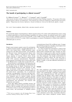
obtained by specifying values of ∆ between 0 and 1. Figure 1 displays the O’Brien-Fleming
and Pocock boundaries for K = 5 equally spaced interim monitoring time-points.
Figure 1: O’Brien-Fleming Stopping and Pocock Stopping Boundaries in the EaSt Software
All these boundaries can be adjusted appropriately by the Lan and DeMets (1983) α-spending
7
function methodology if the actual times at which interm monitoring occurs diﬀer from the
times speciﬁed at the design stage.
In order to obtain the appropriate values for the constants, C(∆, α, K), we must ﬁnd a way to
evaluate the left hand side of equation (2.19) for any speciﬁc choice of the cj ’s. For this we
need to know the joint distribution of {T (t1 ), T (t2 ), . . . T (tK )}. We rely on a very general and
powerful theorem by Scharfstein, Tsiatis and Robins (1997) which may be stated as follows:
Theorem 1 If δˆ is an eﬃcient estimate of δ then, regardless of the model generating the data,
the asymptotic joint distribution of the sequentially computed K-dimensional test statistic
{T (t1 ), T (t2 ), . . . T (tK )} is multivariate normal with mean vector
µT = δ Imax
√
√
√ t1 , t2 , . . . tK
(2.20)
and variance-covariance matrix

VT =
1
  t 1/2

1
 t2

..


.
 1/2
t1
tK
1/2
t
1
t2
1
..
.
t2
tK
1/2
···
···
..
.
···
1/2
t1
t
K 1/2
t2
tK
..
.
1









.
(2.21)
Under the null hypothesis H0 , the mean of this multivariate distribution is µT = 0. The
distribution is thus completely determined and we can solve equation (2.19) in terms of
C(∆, α, K) by means of numerical integration. The numerical integration is considerably
√
simpliﬁed because the special structure of V T implies that tj T (tj ) is a process of
independent increments. This enables us to apply the recursive integration techniques of
Armitage, McPherson and Rowe (1969) and evaluate equation (2.19) very rapidly for a large
family of stopping boundaries parameterized by ∆ . It is important to note that Theorem 1
applies to any probability model generating the data as long as δˆ is an eﬃcient estimate of δ.
Test statistics based on likelihood methods such as Wald tests, score tests, or likelihood ratio
tests are all eﬃcient and ﬁt into this general framework. Thus, whether we have dichotomous
data, normally distributed data, censored survival data or longitudinal data, the same uniﬁed
distribution theory applies in each case.
2.2.2
Derivation of the Inﬂation Factor
Having determined the shape of the stopping boundary, our next task is to evaluate the value
of Imax that will ensure that the study has the desired amount of power 1 − β. This time we
must ensure that for a speciﬁed alternative hypothesis Ha : δ = δa ,
PHa {
K
j=1
|T (tj )| < cj } = β .
8
(2.22)
√ √
√
√ Since, under Ha , µT = δa Imax t1 , t2 , . . . tK , the joint distribution of
{T (t1 ), T (t2 ), . . . T (tK )} is fully determined by the value of
η = δa Imax ,
(2.23)
also known as the drift parameter. We may thus solve equation (2.22) by numerical
integration in terms of the drift parameter, η. Again, the independent increments structure of
V T facilitates the numerical integration. The value of η that solves equation (2.22) will
depend on the coeﬃcient C(∆, α, K) associated with the stopping boundary and on β. Denote
the solution by η(∆, α, β, K). Then, by substitution into equation (2.23),
Imax
η(∆, α, β, K)
=
δa
2
.
(2.24)
Substituting the value of I from the ﬁxed sample equation (2.5) we have
Imax
zα/2 + zβ
=
δa
2
× IF(∆, α, β, K)
(2.25)
where IF(∆, α, β, K), the inﬂation factor, is given by
η(∆, α, β, K)
IF(∆, α, β, K) =
zα/2 + zβ
2
.
(2.26)
These results apply to any model in which a single parameter, δ, captures the primary
endpoint of interest. We may thus use equation (2.25) to convert any ﬁxed sample study into a
corresponding group sequential study. A selection of inﬂation factors for the classical Pocock
and O’Brien-Fleming α-spending functions, for various choices of ∆, α, β and K, are displayed
in Table 1.
Table 1: Inﬂation Factors for Pocock and O’Brien-Fleming (O-F) Alpha Spending Functions
K
2
2
3
3
4
4
5
5
α = 0.05
Spending
Function
Pocock
O-F
Pocock
O-F
Pocock
O-F
Pocock
O-F
(two-sided)
Power (1 − β)
0.80 0.90 0.95
1.11 1.10 1.09
1.01 1.01 1.01
1.17 1.15 1.14
1.02 1.02 1.02
1.20 1.18 1.17
1.02 1.02 1.02
1.23 1.21 1.19
1.03 1.03 1.02
K
2
2
3
3
4
4
5
5
9
α = 0.01
Spending
Function
Pocock
O-F
Pocock
O-F
Pocock
O-F
Pocock
O-F
(two-sided)
Power (1 − β)
0.80 0.90 0.95
1.09 1.08 1.08
1.00 1.00 1.00
1.14 1.12 1.12
1.01 1.01 1.01
1.17 1.15 1.14
1.01 1.01 1.01
1.19 1.17 1.16
1.02 1.01 1.01
2.2.3
Calculators for Translating Fisher Information into Sample Size
It is convenient to express the patient resources needed to achieve the goals of a study in terms
of Fisher information. The calculation is straightforward, requires no knowledge of unknown
nuisance parameters, and facilitates the tabulation of inﬂation factors that can be utilized to
convert ﬁxed sample studies into group sequential ones. But Fisher information is diﬃcult to
interpret in physical terms. For planning purposes, it is necessary to express the patient
resources in a more concrete form such as sample size. However, while a single formula (2.5)
suﬃces for obtaining the Fisher information regardless of the model generating the data, the
same is not true for sample size calculations. Each model requires its own sample size
calculator into which one must input not only the eﬀect size δa , desired power 1 − β, and
signiﬁcance level α, but also our best estimates of unknown nuisance parameters. The EaSt
(2000) software provides such calculators for two-sample tests involving normal, binomial and
survival endpoints, with an inﬂation factor built-in to accommodate interim monitoring. It is
possible to extend these calculators to the family of generalized linear models so as to
accommodate covariates. Many important models including linear regression, logistic
regression, Poisson regression and the Cox proportional hazards model belong to this family.
For logistic and Poisson regression EaSt (2000) provides suitable calculators on the basis of the
theory developed by Self, Mauritsen and Ohara (1992). For very complex survival and
longitudinal designs, sample size is not the only design parameter. Decisions must also be
taken concerning the total study duration, the patient accrual period, the number of repeated
measures for the primary endpoint and the spacing between the repeated measures. In these
complex settings the conversion of Fisher information into a physical resource can be achieved
most eﬀectively through simulation.
2.3
Example 1: Dichotomous Outcome Maximum Information Trial
We wish to design a study to detect a diﬀerence δ = πA − πB between two binomial
populations with unknown response probabilities πA and πB , respectively. The study is to be
designed for up to 4 looks at the data with early stopping based on O’Brien-Fleming 2-sided
level-0.05 stopping boundaries and 90% power to detect a diﬀerence δ = 0.15. Substituting
these design parameters into equation (2.15) and reading oﬀ the appropriate inﬂation factor
from Table 1 we obtain Imax = 477. Thus the monitoring strategy calls for accruing subjects
ˆ −2 equals or exceeds 477 units
onto the study until the total information, as measured by [se(δ)]
or until a stopping boundary is crossed, whichever comes ﬁrst. Notice that in this design, we
did not have to specify the individual values of πA and πB . It was suﬃcient to specify the
clinically meaningful diﬀerence δ for which 90% power was desired.
It is, however, diﬃcult to know how long to accrue subjects when the accrual goals are
expressed in units of square inverse standard error instead of being expressed in terms of a
physical quantity like sample size. We need to translate units of information into sample size
units. This is easy to do since the variance of δˆ is a simple function of the π2 , δ, and the total
10
sample size, N . Thus
ˆ
[se(δ)]
−2
whereupon
(πB )(1 − πB ) (πB + δ)(1 − πB − δ)
+
=
N/2
N/2
−1
= 477 ,
N = 2 × 477 × [(πB + δ)(1 − (πB + δ1 )) + (πB )(1 − πB )] .
(2.27)
(2.28)
It is clear from equation (2.28) that, for the same clinically meaningful diﬀerence δ = 0.15,
diﬀerent values of the baseline probability πB will lead to diﬀerent sample sizes. Based on
historical data we assume that πB = 0.15. Upon substituting this number into equation (2.28),
the required Imax = 477 units of information is translated in Nmax = 323 subjects. Of course, if
the assumption that the baseline response rate is 0.15 is incorrect, then 323 subjects will not
produce the desired operating characteristics. Depending on the actual value of the baseline
response rate we might have either an under powered or over powered study. We now show
that one of the major advantages of the information based approach is that we can use all the
data accrued at any interim monitoring time-point to re-estimate the baseline response rate
and, if it diﬀers from what was assumed initially, re-calculate the sample-size.
Results at the First Interim Monitoring Time-Point
Suppose that at the ﬁrst interim monitoring time point, τ1 , we observe 15/60 responders on
ˆ 1 ) = 0.0167, and
Treatment A and 14/60 responders on Treatment B. Then δ(τ
ˆ 1 )) = 0.0781. The information, I(τ1 ), at the ﬁrst interim monitoring time-point is
se(δ(τ
ˆ 1 ))]−2 = 163.8. Therefore the information fraction at calendar time τ1 is
estimated by se(δ(τ
t1 = I(τ1 )/477 = 0.343. The EaSt (2000) software may now be used to apply the Lan and
DeMets (1983) methodology to the O’Brien-Fleming error spending function at the
information fraction t1 = 0.343. We thereby obtain the corresponding stopping boundary as
ˆ 1 )/se(δ(τ
ˆ 1 )) = 0.21. Since this value
3.47. The observed value of the test statistic is T (t1 ) = δ(τ
is less than 3.47, the study continues on to the next look.
We have accrued 120 subjects out of the 323 required under the design assumption that the
nuisance parameter is πB = 0.15. The information fraction under this design assumption is
thus 120/323 = 0.37, while the actual information fraction is t1 = 0.34. Thus the information
appears to be coming in a little slower than anticipated, but this diﬀerence does not seem
serious enough to alter the sample size requirements of the study.
Results at the Second Interim Monitoring Time-Point
Suppose that at the second interim monitoring time-point, τ2 , we observe 41/120 responders
on Treatment A and 29/120 responders on Treatment B. The information accrued at this time
ˆ 2 ))]−2 = 293.978 and the information fraction is
point is estimated as se(δ(τ
t2 = I(τ2 )/477 = 0.616. The stopping boundary at this information fraction is obtained from
EaSt (2000) as 2.605. The observed value of the test statistic is computed as
ˆ 2 )/se(δ(τ
ˆ 2 )) = 1.715. Since 1.715 < 2.605, the stopping boundary is not crossed and
T (t2 ) = δ(τ
the study continues on to the next look.
This time the anticipated information fraction under the assumption that πB = 0.15 is
240/323 = 0.74, which is considerably larger than the actual information fraction t2 = 0.616.
Thus there is considerable evidence that the information is coming in slower than anticipated.
In fact the data suggest that the value of πB is close to 0.25. It might therefore be prudent to
11
re-estimate the sample size of the study. The new maximum sample size can be obtained by
the relationship
N (τ2 )
I(τ2 )
=
.
Nmax
Imax
Thus the maximum sample size (rounded up to the nearest integer) is
Nmax = N (τ2 ) ×
477
Imax
= 240 ×
= 390.
I(τ2 )
293.978
Therefore we need to commit 390 subjects to the study, not 323 as originally estimated. We see
that the original design with 323 subjects would have led to a seriously under powered study.
Results at the Third Interim Monitoring Time-Point
We continue to accrue subjects beyond the 323 in the original design, and reach the third
interim monitoring time-point at time τ3 with 61/180 responders on Treatment A and 41/180
ˆ 3 ))]−2 = 450.07
responders on Treatment B. At this look the total information accrued is se(δ(τ
and the information fraction is t(τ3 ) = I(τ3 )/477 = 0.943. The observed value of the test
statistic is T (t3 ) = 2.357. The stopping boundary at information fraction t3 = 0.943 is
obtained by EaSt (2000) to be 2.062. Since the observed value of the test statistic, 2.357
exceeds the corresponding stopping boundary, 2.062, the stopping boundary is crossed and the
study terminates with a statistically signiﬁcant outcome.
This example highlights the fundamental diﬀerence between a maximum information study
and a maximum sample size study in a group sequential setting. Had the study been
monitored by the conventional method, the maximum sample size would have been ﬁxed from
the start at 323 subjects and there would have been no ﬂexibility to change the level of this
physical resource over the course of the study. But in an information based approach the
maximum information is ﬁxed, not the maximum amount of a physical resource. Thus the
maximum sample size could be altered over the course of the study from 323 subjects to 390
subjects, while the maximum information stayed constant at 477 units. Without this
ﬂexibility, the power of the study would be severely compromised.
2.4
Example 2: Normal Outcome Maximum Information Trial
Facey (1992) describes a placebo controlled eﬃcacy trial investigating a new treatment for
hypercholesterolemia where the primary response, reduction in total serum cholesterol over a
4-week period, is assumed to be normally distributed. Suppose the goal is to design a four-look
group sequential study having 90% power to detect a reduction in serum cholesterol of 0.4
mmol/litre with a two-sided level 0.05 test. The variance in the cholesterol levels amongst the
subjects in the study is unknown. However we do not need to know the value of this nuisance
parameter to determine the maximum information needed to attain 90% power. Based on
equation (2.15) we can compute the maximum information as Imax = 67.
Although the variance is unknown, we need to make an initial guess at this nuisance
parameter to come up with a preliminary estimate of the maximum sample size. If we assume
12
a balanced design then
ˆ
[se(δ)]
−2
whereupon
4σ 2
=
Nmax
−1
= 67 ,
Nmax = 4 × σ 2 × 67 .
(2.29)
(2.30)
Thus diﬀerent values of σ 2 give diﬀerent maximum sample sizes but the same maximum
information. In fact it is believed that the variance in serum cholesterol levels across patients
on this clinical trial is 0.5. Thus our initial estimate of the maximum sample size is
Nmax = 4 × 0.5 × 67 = 134 patients. We will, however, monitor this trial on the information
scale rather than the sample size scale, so as to avoid dependence on the assumption that
σ 2 = 0.5
Results at the First Interim Monitoring Time-Point
Suppose that at the ﬁrst interim monitoring time-point, there were 35 subjects on the control
arm (arm-C), 34 subjects on the treatment arm (arm-T), x¯C = 4.8, x¯T = 4.58, sC = 0.88,
sT = 0.9. From these observed values we obtain the current information as 21.7775 and the
current value of the test statistic as -0.0267. The information fraction is 21.7775/67 = 0.33.
The O’Brien-Fleming lower stopping boundary at this information fraction is obtained from
EaSt (2000) as -3.571. Since the test statistic has not crossed this lower boundary, the study
continues to the next look. It appears that
√ the standard deviation of the serum cholesterol
levels is somewhat larger than the value 0.5 = 0.707 estimated prior to activating the study.
However as this is only the ﬁrst look at the data it might be preferable to wait for additional
data to accrue before taking a decision to re-estimate the sample size.
Results at the Second Interim Monitoring Time Point
Suppose that at the second interim monitoring time-point, there were 55 subjects on the
control arm (arm-C), 58 subjects on the treatment arm (arm-T), x¯C = 4.75, x¯T = 4.39,
sC = 0.92, sT = 0.95. Based on these numbers we compute the current value of the
information as 32.25 and the current value of the test statistic as -2.0446. We might also revise
the sample-size requirements based on the current estimates of standard deviation. We
actually need a maximum sample size of 236 patients, not 135 as estimated before the study
was activated. This calculation is based on preserving the ratio
n(τ2 )
I(τ2 )
=
.
nmax
Imax
Thus the maximum sample size (rounded up to the nearest integer) is
nmax = n(τ2 ) ×
67.126
Imax
= 112 ×
= 236.
I(τ2 )
32.2553
Notice that although we have accrued 113 patients to the study the cumulative information
fraction is only 0.481. Thus it is clear that unless we increase patient accrual from the initial
speciﬁcation of 135, we will have a seriously underpowered study. Let us assume then that the
investigators agree at this stage to increase the sample size to 236 patients.
Results at the Third Interim Monitoring Time-Point
13
Suppose that at the third interim monitoring time-point nC = 90, nT = 91, x¯C = 4.76,
x¯T = 4.29, sC = 0.91, sT = 0.92. Based on these numbers the current information is 54.04 and
the current value of the test statistic is -3.4551. This time the lower stopping boundary is
-2.249 and so the study terminates with the conclusion that the new treatment does indeed
lower the serum cholesterol level signiﬁcantly relative to the control.
3
Simulation Results
The joint distribution of the sequentially computed test statistics, the derivation of the
stopping boundaries and the computation of the information fraction at each interim
monitoring time-point all depend for their validity on large-sample theory. Therefore in this
section we verify through simulations that the information based design and monitoring
approach discussed in Section 2 does indeed preserve the type-1 error and maintain the power
of a study. We present simulation results for clinical trials with dichotomous outcomes and
clinical trials with continuous, normally distributed outcomes. In both cases we compare the
operating characteristics of maximum information trials with those of maximum sample size
trials. All the trials were designed for 90% power to detect a speciﬁc eﬀect size using 5-look
two-sided O’Brien-Fleming stopping boundaries with a type-1 error equal to 5%.
3.1
Results for Dichotomous Endpoints
Tables 2 and 3 display the power and type-1 error, respectively, for simulations of two-arm
clinical trials with binomially distributed outcomes. Aside from the column headers, each table
contains three rows of simulation results, corresponding to diﬀerent choices of response
probabilities for generating the data. Each table contains six columns. Columns 1, 2, and 3
deal with trials that were designed for an eﬀect size δ = 0.05. The maximum information for
ˆ −2 , it
such studies is computed by equation (2.15) to be Imax = 4316. Since Imax ≈ [se(δ)]
follows that
Nmax = 2Imax [πA (1 − πA ) + πB (1 − πB )] .
(3.31)
Therefore, under the design assumption that πA = 0.1 and πB = 0.05, the maximum
information translates into a maximum sample size of Nmax = 1187 subjects (both arms
combined). Similarly Columns 4, 5 and 6 deal with trials that were designed for an eﬀect size
δ = 0.1 with πA = 0.15 and πB = 0.05. For trials with these input parameters, Imax = 1080 and
Nmax = 378.
The simulation results in Table 2 show that maximum information studies do indeed achieve
the desired 90% power to detect a pre-speciﬁed diﬀerence of δ, regardless of the value of the
nuisance parameter, πB . On the other hand, the actual power of a maximum sample size study
designed for 90% power to detect a pre-speciﬁed diﬀerence of δ, declines if the true value of the
nuisance parameter πB is larger than the value assumed for design purposes, even though
πA − πB = δ.
Let us consider in detail the simulation results displayed in Columns 1, 2 and 3 of Table 2.
Column 1 lists three pairs of response probabilities, (πA = 0.10, πB = 0.05),
14
Table 2: Power Comparison of Maximum Information and Maximum Sample Size Dichotomous
Outcome Clinical Trials: Simulation results for 5-look group sequential trials, using 2-sided
α = 5% O’Brien-Fleming boundaries, designed for 90% power to detect the speciﬁed πA − πB .
Simulation
Design Parameters
Parameters
πA = 0.10, πB = 0.05
(πA , πB )
Max Info
Max Samp
with δ = 0.05 Imax = 4316 Nmax = 1187
(0.10, 0.05)
90.5%
90.5%
(0.15, 0.10)
90.8%
73.4%
(0.20, 0.15)
90.4%
61.3%
Simulation
Design Parameters
Parameters
πA = 0.15, πB = 0.05
(πA , πB )
Max Info
Max Samp
with δ = 0.10 Imax = 1080 Nmax = 378
(0.15, 0.05)
88.7%
90.8%
(0.20, 0.10)
90.5%
77.8%
(0.30, 0.20)
89.8%
60.4%
(πA = 0.15, πB = 0.10) and (πA = 0.20, πB = 0.15), that were used in the simulations. Each
pair satisﬁes the condition πA − πB = 0.05 = δ, which is substituted into equation (2.15) to
obtain Imax = 4316. However, only the ﬁrst of the three pairs also matches the response
probabilities assumed at the design stage and substituted into equation (3.31) to compute
Nmax = 1187. Each row of Column 2 lists the proportion of times in 5000 simulated 5-look
group sequential clinical trials, monitored on the information scale, that the null hypothesis
δ = 0 is rejected, given that the response probabilities (πA , πB ) for the simulations are taken
from Column 1 of the same row. For example, if the simulations are performed with response
probabilities (πA = 0.20, πB = 0.15), then 90.4% of 5000 simulated maximum information
trials reject the null hypothesis. Each row of Column 3 lists the proportion of times in 20,000
simulated 5-look group sequential clinical trials, monitored on the sample size scale, that the
null hypothesis δ = 0 is rejected, given that the response probabilities (πA , πB ) for the
simulations are taken from Column 1 of the same row. For example, if the simulations are
performed with response probabilities (πA = 0.20, πB = 0.15), only 61.3% of 20,000 simulated
maximum sample-size trials reject the null hypothesis.
We now describe how the simulations displayed in Row 3, Columns 2 and Row 3, Column 3 of
Table 2 were carried out. First consider Row 3, Column 3. Each trial starts out with an
up-front sample size commitment of Nmax = 1187 subjects. This sample size ensures that the
study will have 90% power to detect a diﬀerence δ = 0.05, provided the baseline response
probability is πB = 0.05. Since, however, the baseline response probability used for the
simulations is πB = 0.15, the variance of δˆ is much larger that was assumed at the design
stage, and Nmax = 1187 subjects are not suﬃcient for 90% power. This is seen clearly in the
results displayed in Row 3, Column 3 of Table 2 where each simulation is run on the basis of
Nmax = 1187 with no provision to increase this maximum at any of the interim looks. Thus
Row 3, Column 3 shows that only 61.3% of the 20,000 simulations are able to reject H0 rather
than 90% as desired.
Next consider the simulation results displayed in Row 3, Column 2. In these simulated trials
the goal is to accrue as many subjects as are needed to reach Imax = 4316 units of information.
We adopt the following monitoring strategy to achieve this goal. We begin with the initial
assumption that a maximum sample size Nmax = 1187 will suﬃce to attain Imax = 4316. This
15
assumption is based on our initial assessment, made at the time of study design, that the
nuisance parameter πB = 0.05. The maximum sample size is, however, subject to revision as
data from the clinical trial become available at each interim monitoring time-point and provide
a more accurate estimate of the nuisance parameter. We take the ﬁrst interim look at a time
point τ1 , after generating N (τ1 ) = 1187/5 ≈ 238 binomial responses, 119 from πB = 0.15, and
119 from πA = 0.20. We then revise the maximum sample sample size, Nmax , so as to equate
the sample size fraction with the information fraction:
N (τ1 )
I(τ1 )
=
.
Nmax
Imax
We now have a more realistic estimate of the sample size that will be needed to attain
Imax = 4316. The same procedure is adopted at each subsequent interim look and the value of
Nmax is thus altered adaptively until the maximum information is achieved or a stopping
boundary is crossed.
The simulation results in Table 3 show that the type-1 error of both maximum information
and maximum sample size studies is preserved regardless of the value of the nuisance
parameter, πB . These simulations were carried out in the same manner as described above,
but under the null hypothesis πA = πB .
Table 3: Type-1 Error of Maximum Information and Maximum Sample Size Dichotomous Outcome Clinical Trials: Simulation results for 5-look group sequential trials, using 2-sided α = 5%
O’Brien-Fleming boundaries, designed for 90% power to detect the speciﬁed πA − πB .
Simulation
Design Parameters
Parameters
πA = 0.10, πB = 0.05
(πA , πB )
Max Info
Max Samp
with δ = 0 Imax = 4316 Nmax = 1187
(0.05, 0.05)
5.9%
4.8%
(0.10, 0.10)
5.8%
5.1%
(0.20, 0.20)
4.8%
5.0%
3.2
Simulation
Design Parameters
Parameters
πA = 0.15, πB = 0.05
(πA , πB )
Max Info
Max Samp
with δ = 0 Imax = 1080 Nmax = 378
(0.05, 0.05)
4.9%
5.1%
(0.10, 0.10)
6.1%
4.6%
(0.20, 0.20)
5.1%
4.9%
Results for Continuous Normally Distributed Endpoints
Tables 4 and 5 display the power and type-1 error, respectively, for simulations of two-arm
clinical trials with normally distributed outcomes. Aside from the column headers, each table
contains three rows of simulation results, corresponding to diﬀerent choices of σ for generating
the data. Each table contains six columns. Columns 1, 2, and 3 deal with trials that were
designed for data generated from a normal distribution with an eﬀect size δ = 0.2 and a
standard deviation σ = 1. The maximum information for such studies is computed by
ˆ −2 , it follows that
equation (2.15) to be Imax = 270. Since Imax ≈ [se(δ)]
Nmax = 4σ 2 Imax .
16
(3.32)
Therefore, under the design assumption that σ = 1, the maximum information translates into
a maximum sample size of Nmax = 1080 subjects (both arms combined). Similarly Columns 4,
5 and 6 deal with trials that were designed for an eﬀect size δ = 0.4 with σ = 1. For trials with
these input parameters, Imax = 68 and Nmax = 272.
The simulation results in Table 4 show that maximum information studies do indeed achieve
the desired 90% power to detect a pre-speciﬁed diﬀerence of δ, regardless of the value of the
nuisance parameter, σ. On the other hand, the actual power of a maximum sample size study
designed for 90% power to detect a pre-speciﬁed diﬀerence of δ, declines if the true value of the
nuisance parameter σ is larger than the value assumed for design purposes.
Let us consider in detail the simulation results displayed in Columns 1, 2 and 3 of Table 4.
Column 1 lists three values of the nuisance parameter, σ = 1, σ = 1.25 and σ = 1.5, that were
used in the simulations. Only the ﬁrst of these values corresponds to the value of σ that was
actually used to design the study. Each row of Column 2 lists the proportion of times in 5000
simulated 5-look group sequential clinical trials, monitored on the information scale, that the
null hypothesis δ = 0 is rejected, given that the standard deviation σ is taken from Column 1
of the same row. For example, if the simulations are performed with a standard deviation
σ = 1.5, then 90.2% of 5000 simulated maximum information trials reject the null hypothesis.
Each row of Column 3 lists the proportion of times in 20,000 simulated 5-look group sequential
clinical trials, monitored on the sample size scale, that the null hypothesis δ = 0 is rejected,
given that the standard deviation σ is taken from Column 1 of the same row. For example, if
the simulations are performed with a standard deviation σ = 1.5, only 57.7% of 20,000
simulated maximum sample-size trials reject the null hypothesis.
The simulations in Tables 4 and 5 were implemented using the same basic approach discussed
in Section 3.1 for dichotomous endpoints. The details are therefore omitted.
Table 4: Power Comparison of Maximum Information and Maximum Sample Size Normal Outcome Clinical Trials: Simulation results for 5-look group sequential trials, using 2-sided α = 5%
O’Brien-Fleming boundaries, designed for 90% power to detect the speciﬁed δ given σ = 1.
Design Parameters
Simulation
(δ = 0.2), (σ = 1)
Parameters Max Info
Max Samp
(δ = 0.2)
Imax = 270 Nmax = 1080
90.7%
90.1%
(σ = 1.00)
(σ = 1.25)
90.6%
73.2%
(σ = 1.50)
90.2%
57.7%
17
Design Parameters
Simulation
(δ = 0.4), (σ = 1)
Parameters Max Info Max Samp
(δ = 0.4)
Imax = 68 Nmax = 272
(σ = 1.00)
90.3%
89.7%
(σ = 1.25)
90.2%
73.8%
(σ = 1.50)
90.0%
58.1%
Table 5: Type -1 Error of Maximum Information and Maximum Sample Size Normal Outcome
Clinical Trials: Simulation results for 5-look group sequential trials, using 2-sided α = 5%
O’Brien-Fleming boundaries, designed for 90% power to detect the speciﬁed δ given σ = 1.
Design Parameters
Simulation
(δ = 0.2), (σ = 1)
Parameters Max Info
Max Samp
(δ = 0)
Imax = 270 Nmax = 1080
(σ = 1.00)
5.3%
5.1%
(σ = 1.25)
4.8%
5.2%
(σ = 1.50)
5.0%
4.9%
4
Design Parameters
Simulation
(δ = 0.4), (σ = 1)
Parameters Max Info Max Samp
(δ = 0)
Imax = 68 Nmax = 272
(σ = 1.00)
5.6%
5.3%
(σ = 1.25)
5.7%
5.2%
(σ = 1.50)
5.9%
5.3%
Conclusions
When trying to assess treatment diﬀerence in clinical trials, the scientiﬁc objective of the
study can be formulated as the ability to detect clinically important diﬀerences with suﬃcient
precision. We have shown that this precision is directly related to the statistical information in
the data as measured by the magnitude of the standard error of the estimator of treatment
diﬀerence. In general, statistical information is a complicated function of sample size and
nuisance parameters (i.e., parameters in the probability model other than treatment
diﬀerence). However, the amount of information needed to answer the scientiﬁc question is
easily calculated and applies generally to almost any statistical model for a large variety of
endpoints. The general paradigm, currently practiced, is to posit some initial guesses for the
nuisance parameters and then, using the complicated function that relates information to
sample size and nuisance parameters, work out the sample size that leads to the desired
information.
We argue in this article that we should instead be ﬂexible concerning the sample size
requirements, but should focus more on collecting data until we have achieved the desired
information, as estimated by the inverse of the square of the standard error. Such a strategy
would guarantee that we meet the scientiﬁc objective of the study. The diﬃculty with this
approach, is, of course, the logistics of carrying it out. Investigators will not want to launch
into a clinical trial without some sense of how many resources will be needed to carry out the
study. We suggest that the usual strategy of sample size calculations, based on initial best
guesses of the nuisance parameters, be carried out to get some sense of the feasibility of the
study. But the data should be monitored periodically to assess whether the desired
information can be achieved with the proposed sample size. If, during the monitoring process,
it looks as if the initial guesses were incorrect, then the study might be altered appropriately
to meet the information goal necessary to meet the scientiﬁc objective.
Such a strategy is well suited for use in conjunction with a group sequential approach where
the data are routinely monitored anyway. In this context we have described the general large
sample theory of Scharfstein, Tsiatis and Robins (1997) in which sequentially computed test
18
statistics of treatment eﬀect have a common distributional structure that depends only on the
treatment eﬀect parameter and on the statistical information available at the interim
monitoring time-points. This result leads to a general approach to sequential monitoring which
applies to virtually all clinical trials. Consequently, not only are we able to construct stopping
boundaries based on the statistical information estimated at each interim analysis in a simple
and uniﬁed manner, but we can also assess whether the amount of information is what we
would expected based on our initial guesses. In addition, we have the ability to estimate the
nuisance parameters during the interim analysis and, if it seems that the original design will
not meet the goals of the study, we may extend the study, increase the sample size, or make
other adjustments that are necessary to obtain the desired information. As long as we are
monitoring the data and deriving the stopping boundaries on the basis of statistical
information, these adaptive changes will have no eﬀect on the level and power of the
group-sequential test. If we are able to work out the logistics of keeping the clinical trial open
until we have accumulated the desired information, then the power of the test to detect the
clinically important diﬀerence will be achieved regardless of the underlying nuisance
parameters. This would not be the case for strategies using the commonly practiced paradigm
in which a study is terminated once the sample size of the original design is achieved.
Although in this approach one can control the level of the test, the subsequent power of the
test may be greatly aﬀected if the values of the nuisance parameters are guessed incorrectly.
It is also reasonable to adopt information based monitoring for sample size adjustment without
any intention of early stopping. Since regulatory concerns preclude interim monitoring without
spending some type-1 error, one could make this approach operational by adopting extremely
conservative stopping boundaries such as those of Haybittle (1971). In this way there would be
almost no likelihood of stopping early under the null hypothesis, but one would still have the
opportunity to adjust sample size based on the values of the nuisance parameters and the
amount of information actually accrued. In the limit, taking the interim boundaries to inﬁnity
would be equivalent to monitoring only for sample size adjustment.
References
Armitage P, McPherson CK and Rowe BC (1969). Repeated signiﬁcance tests on
accumulating data. J. R. Statist. Soc. A, 132, 232-44.
EaSt: Software for design and interim monitoring of group sequential clinical trials (2000).
Cytel Software Corporation, Cambridge, MA.
Facey KM (1992). A sequential procedure for a Phase II eﬃcacy trial in hypercholesterolemia.
Controlled Clinical Trials, 13, 122-133.
Haybittle JL (1971). Repeated assessment of results in clinical trials of cancer treatment. Brit.
J. Radiology, 44, 793-797.
Kim K and Tsiatis AA (1990). Study duration for clinical trials with survival response and
early stopping rule. Biometrics, 46, 81-92.
Lan KKG and DeMets DL (1983). Discrete sequential boundaries for clinical trials.
19
Biometrika, 70, 659-663.
O’Brien PC, Fleming TR (1979). A multiple testing procedure for clinical trials. Biometrics,
35, 549-56.
Pocock SJ (1977). Group sequential methods in the design and analysis of clinical trials.
Biometrika, 64, 191-99.
Scharfstein DO and Tsiatis AA (1998). The use of simulation and bootstrap in
information-based group sequential studies. Stats. in Med., 17, 75-87.
Scharfstein DO, Tsiatis AA, and Robins JM (1997). Semiparametric eﬃciency and its
implication on the design and analysis of group-sequential studies. JASA, 92, 1342-50.
Self SG, Mauritsen RH, Ohara J.(1992). Power calculation for likelihood ratio tests in
generalized linear models. Biometrics, 48, 31-39.
Wang SK and Tsiatis AA (1987). Approximately optimal one-parameter boundaries for group
sequential trials. Biometrics, 43, 193-99.
20