
809 Financial Education Stephen D. Froikin,
809 Financial Education Stephen D. Froikin, JD, MSEd, ChFC, CLU, CASL, ITP 2701 W. Jarvis Ave. | Chicago, IL 60645 [email protected] 773-480-3051 Finance for Managers 105: Corporate Finance (1st two units) Writing Sample The following are the first two units of a course that I wrote for Kaplan University School of Professional and Continuing Education (© 2014 Kaplan, Inc.). The course is an online course entitled Finance for Managers 105: Corporate Finance. It was written as the fifth part of a series of courses for new managers who lack knowledge of accounting and finance to help them take on their new responsibilities and work effectively with their accounting and finance departments. Only the text portions are reproduced. My video presentations are not included, nor are quizzes, assignments, or exams. Interactive question show the correct answer choice in the first position, marked by an asterisk. In operation, the answer choices are randomized. Each box below represents a separate screen in the online course. —Steve Froikin 809 Financial Education Writing Sample of Steve Froikin Finance for Managers 105: Corporate Finance Unit 1 Overview of Unit 1 Welcome to Unit 1 of your Corporate Finance course. After completing this unit, you should be able to: Explain the use of a time line in preparing a time value of money calculation. Describe factors that influence the selection of an interest rate in a time value of money calculation. Compute the future value of a single sum. Compute the present value of a single sum. Compute the present value of an annuity. Compute the future value of an annuity. Compute the amount of a payment for an annuity. Compute the number of compounding periods for a time value of money problem. Compute the interest rate in a time value of money problem. This unit includes the following tasks: Unit Video Time Value of Money Reading with Practice Problems Microsoft Excel® Workbook Practice Activity PerformIT Microsoft Excel® Workbook Graded Assignment Unit Summary Unit Exam (graded) Approximate Time: 5 hours Tools needed to complete this unit include the following: Microsoft Excel® (2010 version preferred) Adobe Acrobat Reader Unit 1 Presentation Watch the Unit 1 Video presentation. This video will cover some of the key concepts of this unit. Page 2 809 Financial Education Writing Sample of Steve Froikin Page 3 Time Value of Money The central concept in most financial calculations is known as the time value of money (TVM), which is an extension of the idea of compound interest that everyone learns in school. If an individual or a business invests a sum of money today in an account or investment that earns interest, it will grow in a predictable way. What is known as “the magic of compound interest” is the fact that, in a compounding situation, interest is earned not only on the principal amount deposited, but interest is earned on any accumulated interest. The result is growth that is greater than might have been expected, if the investment is held for a period of years. Time value money calculations allow one to determine the future value of a sum invested if you know the interest rate—the future value (FV) calculation. TVM calculations also allow one to go backwards to determine the amount of money one needs to invest today to reach a particular goal—the present value (PV) calculation. Using these tools, it is also possible to calculate the time required for an investment to grow to reach a goal or to determine the interest rate required if the time period is known. The key factors in TVM calculations, then, are: Present value, which is the amount of money at the beginning of a period of time—often abbreviated as PV. Period, which is the time the money is expected to be held—often abbreviated as t (for time), NPER (for number of periods), or simply n (also for number of periods). Interest rate, which is the percentage increment of increase in value per period (usually a year)—often abbreviated as i (for interest), rate (for rate of interest), or simply r (also for rate of interest). Future value, which is the increased value at the end of the period in question—often abbreviated as FV. (The abbreviations noted above are used interchangeably. We thought you should know so that you can interpret these equations regardless of how they are written.) 809 Financial Education Writing Sample of Steve Froikin Page 4 Unit 1 Reality Check This course is designed to extend concepts discussed in courses F4M103 Accounting Essentials and F4M104 Using Accounting Information into the future. Accounting is fundamentally past oriented. It tells you the results of business operations. Time value of money calculations help you make decisions about the future of your b usiness. Before we go on, we’d like to make you aware of the investment terminology you will find in this course. TVM concepts apply to “investments” in the large sense. This includes buying and holding stocks and bonds, of course. But as you learned in F4M104, business firms make internal investment in plant and equipment and all sorts of projects. TVM works on these types of investments as well. The point of the TVM concept is to help you compare two or more projects or investments so that you can make informed decisions about them. For the comparisons to be valid and useful, you must first determine the projected cash flows from the alternative plans, both inflow and outflow. But simply listing these cash flows are not enough, as they usually occur over a period of years. TVM calculations are used to determine the value of the cash flows at some common point in time. This is typically done either at the end of the project or investment, using the FV calculation or at the beginning of the project or investment, using the PV calculation. It is this support for business and investment decisions that makes TVM calculations such powerful tools. These calculations may, at first, appear to be complicated or difficult. Don’t be deterred. Any spreadsheet program will take the complexity away. In this course, we use Microsoft® Excel, which you are already familiar with from previous courses in this program. A little practice will add this powerful method of analysis to your managerial toolkit. The skills you learned in the previous courses were designed to give you professional hindsight. This course gives you your crystal ball. 809 Financial Education Writing Sample of Steve Froikin Page 5 Using a Spreadsheet (or Tables or a Calculator) Before getting into the concepts and procedures, it is important to say that TVM calculations are usually too complex to be done on the back of an envelope. That is not to say that the concepts are difficult, but the calculations generally require repeated procedures that are difficult to keep track of. In the old days, these calculations were accomplished using published tables: compound interest tables (which we call future value), present value tables, annuity tables (when multiple cash flows were involved), loan amortization tables, and so on. These tables are still around, but not used as much as they used to be. Today they are used mostly to give ballpark estimates. Computer-based calculations are generally more precise and flexible. TVM calculations today, are generally accomplished using one of three types of tools: (1) a compute r spreadsheet like, (2) a financial calculator, or (3) an app for a mobile device. Mobile apps offer features of both financial calculators and spreadsheets. Our discussion here will cover the use of the Microsoft® Excel TM spreadsheet, which you have used in the earlier courses in this program. Alternatively, we provide downloadable guidance for using two common financial calculators: HP 12c or TI BA II Plus financial calculators. Click here to access our calculator guide. If your financial tool is not included in the guide, it will be your responsibility to get the users’ manual for your tool. All these tools are similar, but not identical. It is important to become familiar with one or more financial tools. Using a financi al tool allows a student to practice the concepts in this course. It is important to begin to get an intuitive feel of how financial calculations work. Try to estimate results before you enter data. Over time, you will get better with your estimates. This process of estimating and checking will make you more proficient with the calculations. You will know when these concepts are crystallizing in your mind when you begin to have of sense of when you made errors in entering data (a very real possibility) because your results will be way off from your estimate. This process of cross-checking between estimates and actual calculations will be of great help in learning the material. Throughout the course (and in the downloadable calculator guide) the following variables are used. We’ve already talked about most of them. The following table shows the common representation of these variables in calculators or spreadsheets: Variable Meaning N or NPER Number of compounding periods i or I/Y or RATE Interest rate per compounding period PV Present value FV Future value PMT Annuity payments or equal periodic cash flows CPT (or ENTER for spreadsheets) Compute NPV Net Present Value Note: Throughout the problems in this course, rounding differences may occur between t he use of different financial tools presented. So don’t panic if you are a few cents off in your calculations. 809 Financial Education Writing Sample of Steve Froikin Page 6 Time Lines It is often a good idea to draw a time line before you start to solve a TVM problem. A time line is simply a diagram of the cash flows associated with a TVM problem. A cash flow that occurs in the present (today) is put at time zero. Cash outflows (payments) are given a negative sign, and cash inflows (receipts) are given a positive sign. (As discussed in the F4M104 Using Accounting Information discussion of cash flow statements, keeping track of positive and negative signs is absolutely critical and will become even more critical as problems become more complex. Fail in this and you will get the wrong answers.) Figure 1 illustrates a time line for an investment that costs $1,000 today (outflow) and will return a stream of cash payments (inflows) of $300 per year at the end of each of the next five years. Figure 1: Time Line Please recognize that the cash flows occur at the end of the period depicted on the time line. Furthermore, note that the end of one period is the same as the beginning of the next period. For example, the end of the second year (t = 2) is the same as the beginning of the third year, so a cash flow at the beginning of Year 3 appears at time t = 2 on the time line. Keeping this convention in mind will help you keep things straight when you are setting up TVM problems. Interest Rates Are the Measure of the Time Value of Money Interest rates are our measure of the time value of money. Equilibrium interest rates are the required rate of return for a particular investment, in the sense that the market rate of return is the return that investors and savers require to get them to willingly lend their funds. The rate reflects investors’ perceptions of risk. Higher rates generally reflect higher risk and lower rates generally reflect lower risk (assuming the same period of time for holding the investment). Interest rates are also referred to as discount rates and, in fact, the terms are often used interchangeably. If an individual can borrow funds at an interest rate of 10%, then that individual should discount payments to be made in the future at that rate in order to get their equivalent value in current dollars or other currency. Finally, we can also view interest rates as the opportunity cost of current consumption. If the market rate of interest on 1-year securities is 5%, earning an additional 5% is the opportunity forgone when current consumption is chosen rather than saving (postponing consumption). 809 Financial Education Writing Sample of Steve Froikin Page 7 Interest rate as the sum of a real risk-free rate plus a premium for risk The time value of money is always dependent on prevailing interest rates. But interest rates in the market change constantly depending on the type of investment. For purposes of the time value of money, the term investment is not limited to stocks, bonds, or real estate, but can include investments in any type of business project (an internal investment for a firm). The math is the same, which enables a manager to compare projects in the same way one would compare bonds, for example. Interest rates are thought of as made up of various components: a risk-free rate plus premiums for various types of risk. The risk-free rate is quite low and is thought of as the rate that the United States government pays when it borrows. But even the United States is subject to paying higher rates based on perceived risk. Even if you see the United States as 100% safe, market forces do affect your investment in US securities. Starting with the risk-free rate, you add a premium for a variety of types of risk. Here are a few: Business risk. This is the risk to a business from competition, changes in customer preferences, changes in law, poor management, and other factors. This is a significant element for non-financial managers and we will come back to this in Unit 4 of this course. Default risk. This is the risk that a borrower will default on its loans. Inflation risk. This affects the entire economy. Lenders demand a higher rate of interest if they expect inflation to erode the value of any repayment. Liquidity risk. This is the risk that assets won’t bring full value if you are forced to liquidate in a hurry. Maturity risk. This is the risk that the value of longer-term investments may be less sure than short-term investments. Reinvestment risk. This is the risk that, when an investment reaches maturity or a project ends freeing up money, you won’t be able to reinvest at a good rate of return. There are many more risk factors that can go into an interest rate. In evaluating a project in your business, however, you generally use the interest rate your firm would use to borrow money or otherwise raise capital to finance the project. Your finance department should be able to tell you what rate to use for a particular project. We will talk about this topic again in more detail in Unit 4. In the next reading we will try our first TVM calculation. Future Value—Compound Interest Future value is the amount to which a current deposit will grow over time when it is placed in an account paying compound interest. The FV, also called the compound value, is simply an example of compound interest at work. The formula for the FV of a single cash flow is: FV = PV(1 + i) N where: PV = i = N = amount of money invested today (the present value) rate of return per compounding period total number of compounding periods In this expression, the investment involves a single cash outflow, PV, which occurs today, at t = 0 on the time line. The single sum FV formula will determine the value of an investment at the end of N compounding periods, given that it can earn a fully compounded rate of return, i, over all of the periods. The factor (1 + i)N represents the compounding rate on an investment and is frequently referred to as the future value factor, or the future value interest factor, or the compound interest factor for a single cash flow at i over N compounding periods. These are the values that appear in interest factor tables, which we will not be using. 809 Financial Education Writing Sample of Steve Froikin Page 8 Example: FV of a single sum Calculate the FV of a $300 investment at the end of 10 years if it earns an annually compounded rate of return of 8%. Answer: To solve this problem in Excel, use the formula =FV(0.08,10,0,-300). When you began typing the formula, you may have noticed that Excel gives you hints to solving this type of problem. All you have to do is type the beginning of the formula: =FV( and the hints will appear as soon as you hit the open paren. The hint is as follows: FV(rate, nper, pmt, [pv], [type]). This hint is a complete listing of all the variables you will use in TVM problems. As we go further, you will see them appear in different orders, but this is all of them. The ones in brackets are optional for any given problem. The following are the meaning of the variable term and how they are completed for this example Term Meaning Use in this Example FV Future value This is the unknown and is not filled in. RATE Interest rate for the period .08 (this is the stated interest, since we are doing annual compounding) NPER Number of periods 10 (this is the number of years, since we are doing annual compounding, which is the usual way) PMT Amount of any regular interim payments 0 (there are no interim payments, but since this is a mandatory item you enter 0—this will become important later in this unit but is not important now, so long as you enter 0) PV Present value -300 (this is the starting amount of money and is negative since the amount was a cash outflow—although this item is optional, we know the amount and enter it) Type We’ll discuss this later in the Unit This is not filled in. Consequently, the Excel entry is =FV(0.08,10,0,-300), which gives the answer $647.68. This relatively simple problem could also be solved using the following equation: FV = 300(1 + 0.08) 10 = $647.68 But we’re sure you would prefer to do this using Excel, as shown above, or using a calculator. Now you try one. Be sure to read the answer explanation to see how common errors are generated. 809 Financial Education Writing Sample of Steve Froikin Page 9 If your firm invests $250,000 for 15 years at an annually compounded rate of 6.5%, what will be the future value at the end of that time? $642,960* -$642,960 $642.96 $6,045,542 The correct answer is “$642,960.” The Excel formula is: =FV(0.065,15,0,-250000). The other answer options reflect common errors. The negative answer (-$642,960) comes from entering the PV value as a positive number; when PV is negative, FV is positive, and vice versa. The small answer ($642.960) comes from entering the 250000 investment with a comma; always enter formula numbers without commas because Excel uses the comma to separate parts of the formula. The large answer ($6,045,542) comes from entering the 250000 investment as a pmt variable rather than as PV; you have to enter 0 for pmt in this problem and -250000 for PV. 809 Financial Education Writing Sample of Steve Froikin Page 10 Using the Right Interest Rate: Effective Annual Rate In our example and practice problem, interest was stated with annual compounding, but this is not always the case. Although interest is usually stated as an annual rate, compounding is often done more frequently than annually. For example, a bank may quote a savings rate as 8%, compounded quarterly. But 8% compounded quarterly is a better rate than 8% compounded annually. Because of the effect of differing compounding periods, we look to a standard that is known as the effective annual rate (EAR). EAR represents the annual rate of return actually being earned after adjustments have been made for different compounding periods. EAR may be determined as follows: EAR = (1 + periodic rate) m – 1 where: periodic rate = stated annual rate/m m = the number of compounding periods per year To put our example in these terms, we have to say that the EAR for a stated rate of 8% compounded annually is not the same as the EAR for 8% compounded semiannually, or quarterly. Indeed, whenever compound interest is being used, the stated rate and the actual (effective) rate of interest are equal only when interest is compounded annually. Otherwise, the greater the compounding frequency, the greater the EAR will be in comparison to the stated rate. The computation of EAR is necessary when comparing investments that have different compounding periods. It allows for an apples-to-apples rate comparison. Example: Computing EAR Compute EAR if the stated annual rate is 12%, compounded quarterly. Answer: Here m = 4, so the periodic rate is 12 = 3%. 4 Thus, EAR = (1 + 0.03) 4 – 1 = 1.1255 – 1 = 0.1255 = 12.55%. In Excel, the formula for this equation is: =(1+0.12/4)^4-1. The caret symbol is used to create the exponent. (On a financial calculator use the [y x] key.) On the following screens you will have a chance to try this out for practice (your responses will not be scored). Pay attention to the way different compounding periods affect your answers. The change in EAR will be discussed in the explanation to each answer. Quiz Omitted 809 Financial Education Writing Sample of Steve Froikin Page 11 Putting EAR Together with a Future Value Problem The EAR calculation can be used in conjunction with the Future Value calculation (or any other calculation in this unit) simply by following a two-step process: Step One: Calculate EAR Step Two: Calculate Future Value (or any other calculation in this unit) Example: Computing FV When Compounding is More Frequent than Annual Calculate the FV of a $300 investment at the end of 10 years if it earns 8% compounded monthly. Step One: In Excel, the formula for this EAR equation is: =(1+0.08/12)^12-1. This gives an EAR of 8.30% Step Two: In Excel, the formula for this future value equation is: =FV(0.083,10,0 ,-300). This gives FV as $665.90. (If you go back to the first FV example, we computed this same problem using annual compounding. The answer was $647.68. So, you can see that changing from annual to monthly compounding increased the FV.) Many of the problems in this course use annual compounding, but don’t be lulled into complacency. Always pay attention to the frequency of compounding and compute the EAR if necessary. Later in the unit, we will cover an alternative procedure that lets you use compounding periods of less than a year directly. Present Value of a Single Sum The present value (PV) of a single sum is today’s value of a cash flow that is to be received (or paid) at some point in the future. In other words, it is the amount of money that must be invested today, at a given rate of return over a given period of time, in order to end up with a specified FV. In the FV calculation, we know the present value and compute the future value. In the present value computation, we do the reverse. As previously mentioned, the process for finding the PV of a cash flow is known as discounting (i.e., future cash flows are “discounted” back to the present). The interest rate used in the discounting process is commonly referred to as the discount rate but may also be referred to as the opportunity cost, required rate of return, and the cost of capital. Whatever you want to call it, it represents the annual compound rate of return that can be earned on an investment. The relationship between PV and FV can be seen by examining the FV expression stated earlier. Rewriting the FV equation in terms of PV, we get: Note that for a single future cash flow, PV is always less than the FV whenever the discount rate is positive. The quantity 1 / (1 + i)N in the PV equation is frequently referred to as the present value factor, present value interest factor, or discount factor for a single cash flow at i over N compounding periods. 809 Financial Education Writing Sample of Steve Froikin Page 12 Example: PV of a single sum Given a discount rate of 9%, calculate the PV of a $1,000 cash flow that will be received in five years. Answer: To solve this problem, we use the PV function in Excel, using the following values: RATE: 0.09 NPER: 5 PMT: 0 (remember this!) FV: 1000 (enter as a positive number, as the problem states this amount will be received as a cash inflow) This will appear as: =PV(0.09,5,0,1000) and gives you the answer: -$649.93. Note: It is common practice to ignore the positive and negative signs associated with cash flows in these types of problems, but it is a bad habit and will cause you difficulties when you get to problems with multiple cash flows later in this course. This relatively simple problem could also be solved using the following PV equation: As you can see, the Excel formula (or comparable formulas for a financial calculator or other spreadsheet or app) are much simpler method for solving these types of problems. The PV computed in this example implies that at a rate of 9%, an investor will be indifferent between $1,000 in five years and $649.93 today. Put another way, $649.93 is the amount that must be invested today at a 9% rate of return in order to generate a cash flow of $1,000 at the end of five years. And you can see that PV is the reverse of the FV calculation by doing an FV calculatio n using the $649.93 as the starting value for PV. Enter the following into Excel: =FV(0.09,5,0,-649.93) and get the answer: $1000.00! Now try one yourself. How much would you have to deposit today a 6% interest to have $30,000 at the end of 8 years? $18,822.37* $186,293.81 $186.29 $18,905.09 The correct answer is “$18,822.37.” Enter the following present value formula into Excel: =PV(0.06,8,0,30000). The answer is -$18,822.37. The question did not ask for the “cash flow,” which would have required a negative answer. The question asks for the “deposit,” which implies a negative cash flow already. The incorrect answer choices represent answers that result from entering the data into the Excel formula in the wrong order or by entering a comma in the $30,000. 809 Financial Education Writing Sample of Steve Froikin Page 13 Annuities—Stream of Equal Cash Flows An annuity is a stream of equal cash flows that occurs at equal intervals over a given period. Receiving $1,000 per year at the end of each of the next eight years is an example of an annuity. Annuities are frequently used as a model of a business project because business projects are generally designed to generate reliable str eams of income. (The hoped-for cash flows may not be exactly equal, but for purposes of planning, equal cash flows are often assumed.) Typically, you want to know the present value (PV) of that stream of income to see if it is worth the investment. Before getting to the calculation itself, you should know that there are two types of annuities: ordinary annuities and annuities due. The ordinary annuity is the most common type of annuity. It is characterized by cash flows that occur at the end of each compounding period. This is a typical cash flow pattern for many investment and business finance applications. It is the default calculation that occurs in your spreadsheet or calculator. (This is the “type” variable we mentioned above; you don’t have to set this variable for an ordinary annuity because ordinary annuities are the default.) The other type of annuity is called an annuity due, where payments or receipts occur at the beginning of each period (i.e., the first payment is today at t = 0). (We will work o n ordinary annuities first, and then show you how to set the type variable for annuities due.) Computing the PV or FV of an annuity Computing the PV or FV of an annuity with your spreadsheet is no more difficult than it is for a single cash flow. You will know four of the five relevant variables and solve for the fifth (either PV or FV). The difference between single sum and annuity TVM problems is that instead of solving for the PV or FV of a single cash flow, we solve for the PV or FV of a stream of equal periodic cash flows, where the size of the periodic cash flow is defined by the payment (PMT) variable on your spreadsheet or calculator. Example: PV of an ordinary annuity What is the PV of an annuity that pays $200 per year at the end of each of the ne xt 13 years, given a 6% discount rate? Answer: The payments occur at the end of the year, so this annuity is an ordinary annuity. To solve this problem, we use the present value formula in Excel that we saw before, but we now use the PMT variable (rather t han set it at 0, as we did before). To start with, let’s take a look at the variables: RATE: 0.06 NPER: 13 PMT: 200 FV: 0 or omit (When the annuity is completely paid out there is nothing left as a future value. This is an optional variable; you will get the same answer whether you omit this or enter 0.) Type: 0 or omit (0 corresponds to an ordinary annuity, which pays at the end of each period. But this is the default value, so you may omit this. If you want to enter a type variable, you may not omit the F V variable.) This Excel formula will therefor appear as: =PV(0.06,13,200,0,0) and gives you the answer: -$1,770.54. Note that the PMT variable is entered as a positive number because the $200 payments are cash inflows. This causes the PV to be negative, because this represents the amount you would invest in the annuity, which is a cash outflow. 809 Financial Education Writing Sample of Steve Froikin Page 14 Example: PV of an ordinary annuity beginning later than t = 1 What is the present value of four $100 end-of-year payments if the first payment is to be received three years from today and the appropriate rate of return is 9%? Answer: The time line for this cash flow stream is shown in the following figure. PV of an annuity with payments beginning at t = 3 This is like the previous example, if we assume the annuity was purchased at t = 2. This becomes a two-step process, in which we find the present value of a four-year annuity at t = 2. And then we discount it as a single-sum to t = 0. Step 1: Find the present value of the annuity as of the end of year 2 (PV 2 ). Input the relevant data and solve for PV 2. In Excel, enter =PV(0.09,4,100). The answer for PV 2 is -$323.97. (Remember that Excel gives a negative value for PV if the PMT (or FV) is positive. But this is an intermediate value and not an actual cash flow, so we will enter a positive value in the next step.) Step 2: Find the present value of PV 2, which we will call PV0. In Excel, enter =PV(0.09,2,0,323.97). This gives a value for PV 0 of -$272.68. Now you try one. A bond will make coupon interest payments of $70 at the end of each year and will also pay its face value of $1,000 at maturity in five years. If the appropriate discount rate is 8%, what is the present value of the bond’s promised cash flows? (This is a bit of a curve, but if you look at the Excel formula, you will get the answer.) -$960.07 -$401.09 -$1,129.26 -$280.17 The correct answer is “-$960.07.”The five annual coupon payments of $70 each can be viewed as an ordinary annuity. The maturity value of 1,000 euros is the future value of the bond at the time the last coupon payment is made. Excel allows you to input this future value along with the periodic payments. Remember that the PV formula is =PV(rate,nper,pmt,fv). Previously, we omitted the FV value or entered 0, but now we have a future value and there is a perfect spot for it. So to solve this problem, we enter =PV(0.08,5,70,1000) and get -$960.07. This is the price you would pay for this bond today. We want to warn you about two of the incorrect answers. Incorrect answer -$401.09 comes from entering PMT as negative while FV is positive. PMT and FV have to be the same sign. Incorrect answer -$280.17 comes from entering the $1,000 maturity value with a comma. Remember that commas separate the different values in the formula so they can’t be used within a number. 809 Financial Education Writing Sample of Steve Froikin Page 15 Future Value of an Annuity Due Early in this discussion, we mentioned the difference between an ordinary annuity and an annuity due. The ordinary annuity is an annuity with payments at the end of a period. The annuity due is an annuity with payments at the beginning of a period. In our PV-of-an-annuity examples we just completed, we used ordinary annuities. This pairing of the PV calculation with ordinary annuities is pretty common. Present value of an annuity due is an odd, but not impossible situation, which makes it less common. Now, as we turn to finding the future value of an annuity, we find that the common FV situation is FV of an annuity due (FVAD). (Future value of an ordinary annuity is definitely possible, but less frequent.) In Excel, use the [type] term in the formula and set the value to 1. Type 1 sets the payment for the beginning of the period. Type 0 sets the payment for the end, as we noted before. Type 0 is the default. If no type is indicate, it will be assumed that payments are at the end of each period. The following example illustrates how to compute the FV of an annuity due. Think about why the annuity due is the common scenario for computing the future value of an annuity. Example: FV of an annuity due If you deposit $1,000 in the bank today and at the beginning of each of the next 10 years, how much will you have 10 years from today at 6% interest? The time line for this problem is shown in the following figure. Answer: FV of an Annuity Due Note that, since the deposits start immediately, the 10th deposit will occur at the end of the ninth year (which is the same as the beginning of the 10th year). In Excel, the variables are as follows: RATE: 0.06 NPER: 10 PMT: -1000 (no commas; negative because it is a cash outflow) PV: 0 (Don’t enter 1000 because that would result in double counting. This is an annuity due, which means the payments are made at the beginning.) Type: 1 (1 = annuity due) This Excel formula will therefor appear as: =FV(0.06,10,-1000,0,1) and gives you the answer: $13,971.64. Now you try one. 809 Financial Education Writing Sample of Steve Froikin Page 16 If you deposit $12,000 per year in an account that pays 5% starting on your 50th birthday, how much will you have in the account on your 62nd birthday? $200,555.79* -$200,555.79 $48,448.19 $85,382.27 The correct answer is “$200,555.79.” In Excel enter: =FV(0.05,12,-12000,0,1) and get $200,555.79. 809 Financial Education Writing Sample of Steve Froikin Page 17 Present Value of a Perpetuity A perpetuity is an investment that pays a fixed amount of money at set intervals over an infinite period of time. In essence, a perpetuity is a perpetual annuity. In the investment world, preferred stocks are examples of perpetui ties since they promise fixed dividend payments indefinitely. A business project may also project income for an undefined (hopefully long) period of time. Without going into all the excruciating mathematical details, the present value of a perpetuity is si mply the amount of the annual payment divided by the interest rate, as shown in the following equation: In Excel, there is no special formula like there is for the other TVM calculations because this is so simple. Just divide the payment amount by the interest rate. But, if you forget this, you can trick Excel to approximate the value using the PV formula by simply using a very large number for NPER. The larger the number, the closer you will get to the true answer. (Because of rounding, you won’t have to go too high. Try larger and larger numbers until the answer stops changing.) Finding the Amount of a Payment So far, we’ve talked about finding the present or future values of a sum of money or series of payments. Is it possible to find the amount of a payment if you know the present or future value? Of course it is! This is a very useful calculation if you want to figure your payments if you want to borrow some money (i.e., you know the present value, which is the amount of the loan) or if you want save to reach a specific goal (i.e., you know the future value, which is the goal amount). Let’s see how it works. Example: PMT on a loan You need to borrow $15,000 to purchase a 3D printer. You want to pay it off in 5 years. Your supplier will charge you 9% interest. How much will the payments be? In Excel, we use the same group of variables we used in the FV or PV calculations, but this time we solve for PMT. The variables are: RATE: 0.09 NPER: 5 PV: 15000 (This is positive because borrowing $15,000 is a cash inflow, even if you immediately spend the money on the printer.) FV: 0 or omit (You owe nothing at the end of the 5 years.) Type: 0 or omit (Payments are made at the end of the period, which is the default or is indicated by 0.) This Excel formula will therefor appear as: =PMT(0.09,5,15000) and gives you the answer: -$3,856.39. The answer is negative because a loan payment is a negative cash flow. Now you try one. 809 Financial Education Writing Sample of Steve Froikin Page 18 You need to borrow $96,000 to open a branch office in Stockton, CA. You get a 7-year loan at 6.5%. What will your payments be? $17,503.81* $11,263.81 $18,885.81 $149,182.71 The correct answer is “$17,503.81.” In Excel enter: =PMT(0.065,7,96000) and get -$17,503.81. The minus sign indicates that the amount is a cash outflow. Since we asked the amount of the payment, it is customary to leave off the minus sign. Loan Payments and Amortization The equal payment plans we have just calculated are called loan amortization. The whole idea of loan amortization is that payments are equal, and that is what makes the PMT calculation work. The fact of the matter is that every loan payment can be seen as partly interest and partly principal. Since interest payments are often tax deductible but principal payments are not, it is often important to break each p ayment into its interest and principal components. Let’s look at an example to see how it is done. 809 Financial Education Writing Sample of Steve Froikin Page 19 Example: Constructing an amortization schedule Construct an amortization schedule to show the interest and principal components of the end -of-year payments for a 10%, 5-year, $10,000 loan. Answer: The first step in solving this problem is to compute the amount of the loan payments. In Excel, enter: =PMT(0.1,5,10000) and get: -$2,637.97. This means the loan will be repaid via five equal $2,637.97 end-of-year payments. Each payment is made up of an interest component (profit to the lender) plus the partial recovery of loan principal, with principal recovery being scheduled so that the full amount of the loan is paid off by the end of Year 5. The exact a mount of the principal and interest components of each loan payment are presented and described in the amortization table shown below. Amortization Table Period Beginning Balance Payment Interest Component (1) Principal Component (2) Ending Balance (3) 1 $10,000.00 $2,637.97 $1,000.00 $1,637.97 $8,362.03 2 8,362.03 2,637.97 836.20 1,801.77 6,560.26 3 6,560.26 2,637.97 656.03 1,981.94 4,578.32 4 4,578.32 2,637.97 457.83 2,180.14 2,398.18 5 2,398.18 2,638.00 * 239.82 2,398.18 0.00 * There is usually a slight amount of rounding error that must be recognized in the final period. The extra $0.03 associated with payment five reflects an adjustment for the rounding error and forces the ending balance to zero. 1. Interest component = beginning balance × periodic interest rate. In period 3, the interest component of the payment is $6,560.26 × 0.10 = $656.03. 2. Principal component = payment – interest. For example, the period 4 principal component is $2,637.97 – $457.83 = 2,180.14. 3. The ending balance in a given period, t, is the period’s beginning balance minus the principal component of the payment, where the beginning balance for period t is the ending balance from period t – 1. For example, the period 2 ending balance equals $8,362.03 – $1,801.77 = $6,560.26, which becomes the period 3 beginning balance. Note: Once you have solved for the payment, $2,637.97, the remaining principal on any payment date can be calculated by entering N = number of remaining payments and solving for the PV. 809 Financial Education Writing Sample of Steve Froikin Page 20 Using Excel to Construct an Amortization Schedule In Excel, you can create the table we saw on the previous screen as follows (we are showing the formulas, rather than the answers, here): (Recall that the problem asked: Construct an amortization schedule to show the interest and principal components of the end-of-year payments for a 10%, 5-year, $10,000 loan.) <Insert F4M105_Image8.jpg> Notes: First, the formula in cell C2 is the same one we used above, except we supply the PV by reference to the Beginning Balance value in cell B2. Second, all the values in column C could be =C2 because the definition of an amortized payment is that the payments are all the same. We created this spreadsheet, however, by pasting the formulas from row 3 into the remaining rows. When this is done, Excel automatically advances the row element of all the cell references. This technique is very helpful in columns D, E, and F because it saves retyping the formulas. It doesn’t matter in row C because all the values in this column are equal to each other. Column D computes interest by multiplying the interest rate by the beginning balance for that period, which is in column B. This is subtracted from the payment amount (C) to give the principal component in C olumn E. The principal amount (E) is subtracted from the beginning balance (B) to give the ending balance in Column F. Finally, the results of these computations closely match the chart above but may be off a few pennies. This is due to the different ways different programs handle rounding errors and should not be worried about. Let’s leave the amortization table for now and return to it when you tackle the Workbook. Let’s move on to another practical scenario. 809 Financial Education Writing Sample of Steve Froikin Page 21 Example: Annual savings amount to achieve a future goal You expect to need $150,000 in 5 years. How much do you need to deposit at 7% to achieve this goal? To solve this in Excel, the variables are: RATE: 0.07 NPER: 5 PV: 0 (You are starting with nothing.) FV: 150000 (This is your goal amount. It will be a positive cash flow when you withdraw the money.) Type: 1 (You are making the deposits at the beginning of the period. Type 1 = beginning.) This Excel formula will therefor appear as: =PMT(0.07,5,0,150000) and gives you the answer: -$26,083.60. Your annual deposit will be $26,083.60. Example: Monthly savings amount to achieve a future goal Let’s say you would prefer to make these deposits in monthly installments rather than yearly. You can’t just divide the annual amount by 12, because each monthly deposit starts earning interest when it is made. You have to recalculate based on 60 monthly payments (12 x 5 = 60) and you need to use a monthly, rather than annual interest rate (7% divided by 12 = 0.58333%). To solve this in Excel, the variables are: RATE: 0.07/12 (You can enter the fraction for the rate, just as it is shown here.) NPER: 5*12 (You can enter the multiplication for NPER, just as it is shown here.) PV: 0 (You are starting with nothing, same as before.) FV: 150000 (This is your goal amount, also the same as before.) Type: 1 (You are making the deposits at the beginning of the period. Same as before.) This Excel formula will therefor appear as: =PMT(0.07/12,5*12,0,150000) and gives you the answer: -$2,095.18. Your monthly deposit will be $2,095.18 Now you try one. How much would you have to save on a monthly basis to be able to make a $40,000 down payment on a house in five years if you are able to earn 5.5% on the money? $580.71* $92.28 $7,167.06 $7,927.00 The correct answer is “$580.71.” In Excel, the formula is: =PMT(0.055/12,5*12,0,40000) and you get -$580.71 (the minus indicates that the $580.71 is a deposit, not a withdrawal). The key to this calculation is that you divide the annual interest rate by 12 to get the interest rate for the period in questions (i.e., monthly) AND you multiply the number of years by 12 to get the number of months (which is the period in question). If you did only one of these things or neither, you got one on the incorrect answer choices. 809 Financial Education Writing Sample of Steve Froikin Page 22 Computing the Time Element You should now be getting comfortable with the time value of money functions in Excel (financial calculators work in a similar way). You should have noticed that, in computing PV or FV or PMT, we basically reshuffled the variables. We input the known values and the program computes the unknown value. We’re going to continue on that theme as we look at computing NPER and RATE. Up until now, these variables have been given to you, but they can be computed as well. Let’s first look at computing NPER. Example: Computing the number of periods in an annuity How many $100 payments are required to accumulate $1,000 if the discount rate is 9%? Answer: In Excel, we use the NPER formula to solve this problem. The variables are: RATE: 0.09 PMT: -100 (Remember the sign convention. PMT and FV must have opposite signs—one is a deposit and the other is a withdrawal. If you fail to do this, you will either get a nonsense answer, like a negative number of years, or an error message.) PV: 0 (We started with nothing.) FV: 1000 Type: 1 (If you plan to start a savings plan immediately, you need to indicate that the payments are at the beginning of the period.) This Excel formula will therefor appear as: =NPER(0.09,-100,0,1000,1) and gives you the answer: 6.985, which we will call 7 years (in exactly 7 years you would have $1,002.85, which will allow you to buy a cup of coffee and pocket the $1,000). Now you try one. Suppose you bought an annuity earning an 8% return for $1,000. How many annual end-of-year $150 withdrawals can be made? 9.9* -5.5 5.5 8.8 The correct answer is “9.9.” In Excel, the formula is: =NPER(0.08,150,-1000) and you get 9.9029. This is basically 10 years, but the last payment would fall short of $150 by a tiny amount. The negative incorrect answer was the result of not entering the PMT value and the PV value with opposite signs. 809 Financial Education Writing Sample of Steve Froikin Page 23 Computing the Rate The final variable we will be computing is RATE. In the next unit, this variable will be important together with PV. Two ways of comparing investment or projects are either to compare their rates of return or to compare their present values based on a common assumed rate of return. The next unit will use these factors to evaluate uneven cash flows, which are typical in business, but more complicated than what we have done in this unit. For this unit, we will close by looking at how we compute RATE based on even cash flows —the same scenario we have been doing throughout this unit. Let’s look at an example. Example: Computing the rate of return for an annuity What rate of return will you earn on an ordinary annuity that requires a $70,000 deposit today and promises to pay $10,000 per year at the end of each of the next 10 years? Answer: In Excel, we use the RATE formula to solve this problem. The variables are: NPER: 10 PMT: 10000 (This is an amount received, so it is positive.) PV: -70000 (This is an amount paid, so it is negative.) FV: 0 or omit (There is nothing left after the annuity is paid out. FV is an optional variable, s o you can omit it, unless you need to enter it as a place holder so that you can enter the annuity type. That is not required here.) Type: 0 or omit (The payments in this problem are at the end of the period, so you can enter 0 —if you entered a value for FV—or you can omit this variable.) Guess: omit (Excel and other programs use a guess-and-check algorithm to solve RATE problems. You may enter your own guess to help out. If you don’t, Excel will supply its own guess to get the process started. A guess is not required for this problem, but might be valuable for more complicated problems, which we will get to in Unit 2.) This Excel formula will therefor appear as: =RATE(10,10000,-70000) and gives you the answer: 7.07%. Now you try one. Your company is opening a new product line. Startup costs are $150,000 as of today. You expect that the net income (Gross profit minus all expenses) will be $25,000 per year for 7 years. What is the rate of return? 4.01%* Data is insufficient 8.05% 16.67% The correct answer is “4.01%.” In Excel, the formula is: =RATE(7,25000,-150000) and you get 4.01% as the rate of return. This is a very simplified form of the type of problems we will see in Unit 2. We assume that the startup costs are incurred on a single day and are analogous to the payment for an annuity, so we enter it as PV. We also assume that net income is analogous to the regular stream of annuity payments, so we enter it as PMT. 809 Financial Education Writing Sample of Steve Froikin Page 24 Unit 1 Workbook Practice Workbook Practice Activity It is time to put into practice what we have learned in Unit 1. Please complete the following actions in order to practice your knowledge. 1. Download/save the Corporate Finance Workbook to your computer. Save this document in a place where you will be able to find it again, as you will use this workbook in other units of this course. You may also wish to save it for quick reference after you complete the course. 2. Select the Unit 1 tab. 3. Review the “Prepare” material at the top of the Unit 1 spreadsheet. 4. Complete the activities presented under “Practice” in the Unit 1 spreadsheet. Make sure you have completed all the activities in the Unit 1 spreadsheet as they will provide solid preparation for performing well on the Unit 1 graded assignment, which is the next task you will complete. Graded Assignment Omitted 809 Financial Education Writing Sample of Steve Froikin Page 25 Unit 1 Summary Unit 1 covers fundamental time value of money concepts. In this unit you learned: The use of a time line in preparing a time value of money calculation. Creating a sketch showing all cash flows, positive and negative, plotted against time is very useful in understanding a compound interest situation, allowing you to plan the required calculations. Factors that influence the selection of an interest rate in a time value of money calculation. Interest is charged for the use of money for a period of time. There is a charge even if the investment is 100% safe, but the charge (i.e., the interest) is higher if there is a risk that the money might not be repaid. So premiums are added to the risk-free rate to cover various types of risk. How to compute the future value of a single sum. The future value of a single sum is the amount that will result in the future when a given amount is invested today at a given rate of interest. Methods for handling this calculation using a spreadsheet were given. How to compute the present value of a single sum. The present value of a single sum is the amount that must be invested today at a given rate of interest to achieve a financial goal. Methods for handling this calculation using a spreadsheet were given. How to compute the present value of an annuity. The present value of an annuity is the amount that must be invested today at a given rate of interest to generate a stream of regular equal payments. Methods for handling this calculation using a spreadsheet were given. How to compute the future value of an annuity. The future value of an annuity is the amount that will result when a regular stream of equal payments are invested at a given rate of interest. Methods for handling this calculation using a spreadsheet were given. How to compute payment amounts in an annuity. The payment is the amount that will be received on a regular basis when a sum is invested at a given rate of interest. Alternatively, the payment is the amount that must be invested on a regular basis at a given rate of interest to achieve a financial goal. Methods for handling this calculation using a spreadsheet were given. How to compute the number of compounding periods for a time value of money problem. The compounding period in a time value of money calculation can be computed if all other variables are known. Methods for handling this calculation using a spreadsheet were given. How to compute the interest rate in a time value of money problem. The interest rate in a time value of money calculation can be computed if all other variables are known. Methods for handling this calculation using a spreadsheet were given. Unit Exam Omitted 809 Financial Education Writing Sample of Steve Froikin Finance for Managers 105: Corporate Finance Unit 2 Overview of Unit 2 Welcome to Unit 2 of your Corporate Finance course. After completing this unit, you should be able to: Compute present and future value of a series of unequal cash flows. Calculate the net present value (NPV) of a project's cash flows. Compute the internal rate of return (IRR) of a project's cash flows. Compare the NPV and IRR decision rules. This unit includes the following tasks: Unit Video Time Value of Money Readings with Practice Problems Microsoft Excel® Workbook Practice Activity PerformIT Microsoft Excel® Workbook Graded Assignment Unit Summary Unit Exam (graded) Approximate Time: 5 hours Tools needed to complete this unit include the following: Microsoft Excel® (2010 version preferred) Adobe Acrobat Reader Unit 2 Presentation Watch the Unit 2 Video presentation. This video will cover some of the key concepts of this unit. Page 26 809 Financial Education Writing Sample of Steve Froikin Page 27 Unequal Cash Flows In Unit 1, you learned the basic time value of money calculations, in particular, calculations to determine present value, or future value, or payment amounts of a stream of equal payments over a period of time. We noted there briefly that many business situations involve streams of payments that are unequal. This unit builds on your knowledge from the last unit to give you a method for evaluate unequal cash flows. All the elements of this unit’s calculations are the same and have the same meaning: Present value is the amount of money at the beginning of a period of time—often abbreviated as PV. Period is the time money is expected to be held—often abbreviated as t (for time), NPER (for number of periods), or simply n (also for number of periods). Interest rate is the percentage increment of increase in value per period (usually a year) —often abbreviated as i (for interest), rate (for rate of interest), or simply r (also for rate of interest). Future value, which is the increased value at the end of the period in question—often abbreviated as FV. Furthermore, the calculation methods for these factors are also the same. Two things are new in this unit: The general theoretical method for combining time value of money calculations for unequal cash flows; and A streamlined technique for computing “net present value (NPV)” for multiple positive and negative cash flows and the relating “internal rate of return (IRR),” which will be your key for evaluating business projects. Reality Check The key to this unit are the Net Present Value (NPV) and Internal Rate of Return (IRR) calculations. They are really two sides of the same coin. NPV gives you a tool for evaluating a project in doll ars and cents. IRR does the same thing in terms of a percentage. There are pros and cons to either of them, which we will cover in this unit. The thing you want to keep in mind about both of these calculations is that they are not exact. How could they be? All the input to these calculations are estimates—guesses really. You are going to try your best to estimate a stream of cash outflows (initial investment, future costs of labor and materials, marketing, etc.) and a stream of cash inflows (sales, savings compared to existing processes, etc.). Then you pop these values into the NP V or IRR formulas. Running guestimates through a math formula does not make them foolproof. The best you can probably do is make up multiple sets of guesses: high, medium, and low to see what the risks are and the possible benefits. These formulas merely speed the analysis. They don’t make it any more correct than the input data. Before moving onto the material, there is one more point to remember. In Unit 1, we stressed the importa nce of entering cash inflows as positive and cash outflows as negative. The truth is that, in simple problems like we encountered in Unit 1, we could have been more relaxed about it. If you failed in Unit 1 to enter a negative value for PV, you simply get a negative value for FV. You can correct that in your head. With multiple cash flows, however, there’s no easy recovery from mixing up cash inflows with cash outflows. That’s why we stressed the point in Unit 1—to get you in the habit. And we stress it even more in this unit: don’t get the positives and the negatives mixed up. Always use the correct sign. 809 Financial Education Writing Sample of Steve Froikin Page 28 PV and FV of Uneven Cash Flow Series It is not uncommon to have applications in investments and corporate finance where it is necessary to evaluate a cash flow stream that is not equal from period to period. The time line here depicts such a cash flow stream. Time Line for Uneven Cash Flows This 6-year cash flow series is not an annuity since the cash flows are different every year. In fact, there is one year with zero cash flow and two others with negative cash flows. In essence, this series of uneven cash flows is nothing more than a stream of annual single sum cash flows. Thus, to find the PV or FV of this cash flow stream, all we need to do is add up the PVs or FVs of the individual cash flows. 809 Financial Education Writing Sample of Steve Froikin Page 29 Example: Computing the FV of an uneven cash flow series Using a rate of return of 10%, compute the future value of the 6-year uneven cash flow stream described above at the end of the sixth year. Here is that timeline again. Answer: The FV for the cash flow stream is determined by first computing the FV of each individual cash flow, then totaling the FVs of the individual cash flows. Recall that, in Excel, the formula for future value is =FV(RATE,NPER,PMT,PV,TYPE). The values we are using for these variables are: RATE: 0.1 NPER: Varies. Each cash flow has a different period. The year 1 cash flow has 5 years until year 6, the year 2 cash flow has 4 years until year 6 and so on. PMT: 0. This is not an annuity (series of regular payments) so we use 0 to reflect the fact that there are no annuitytype payments. PV: Varies. Each cash flow is a different amount. TYPE: Omit. TYPE is an irrelevant variable if there are no annuity payments. Note that both NPER and PV are marked “Varies.” We can use the power of Excel to fill these two variables automatically. Here is how it is done: We entered data for Cash Flow and Years Till Year 6 in the shaded cells. We also entered the FV formula o nce in shaded cell D1. We supplied the values for RATE and PMT, noted above. But for the variable values, we referred to the values we entered in columns B and C. So, for NPER, we entered C2, which tells Excel that the value we want for NPER is found in the C2 cell (that is, NPER is 5). For PV, we tell Excel to go to the B2 cell (that is, PV is -1000). Notice that we used a minus sign before B2. This is because know that the FV value has to appear as a cash outflow (i.e., it is a loss). In order to do this, we have to reverse the sign of PV. Why did we enter the B2 and C2 references in the formula, rather than entering the numbers themselves? Because we can now copy the formula in the cells below D2 and Excel automatically updates the cross references, so th at the formula can pick up the values of B3 and C3, or B4 and C4, etc. This is a handy technique for keeping everything straight when you have multiple cash flows. 809 Financial Education Writing Sample of Steve Froikin Page 30 (Excel doesn’t really let you keep formulas out in the open like this. We forced it into thi s display mode for illustration purposes.) The result of these individual-cash-flow calculations is shown in column E. Notice that our plan of using a minus sign for the PV values (-B2, -B3, -B4, etc.) worked and the signs for each result in column E match the sign of each cash flow in column B. The final step in the process is to add all the individual FV values. We do that using Excel’s SUM function, and we specify the cells we want summed as E2:E7, which means “every cell starting with E2 and ending with E7.” Now you try one. What is the present value of this 6-year uneven cash flow stream described above using a 10% rate of return? $5,953.75* $8,598.38 $40,462.45 $10,547.44 The correct answer is “$5,953.75.” This is calculated in a similar manner to the FV problem we just illustrated. This time the formula is the present value formula: =PV(RATE,NPER,PMT,[FV], [TYPE]). The fixed variables are RATE = 0.1; PMT = 0; and TYPE is irrelevant without annuity payments. NPER is the number of years between the year of the cash flow and year 0. FV is the cash flow indicated in the problem, but remember to reverse the sign of each cash flow so the FV matches the sign of the cash flows shown in the problem. The answer is the total of all the individual PV values. 809 Financial Education Writing Sample of Steve Froikin Page 31 Calculating the Net Present Value (NPV) of a Project’s Cash Flows The process of calculating the present value of a series of uneven cash flows is so useful in evaluating business projects that a simplified method is often used in place of the method we have shown you. It is called net present value. The “present value” part you already know. The “net” simply indicates that all the positive and negative PV values are added up to arrive at a net figure. Here is the formal definition of this concept: The net present value (NPV) of an investment project is the present value of expected cash inflows associated with the project less the present value of the project’s expected cash outflows, discounted at the appropriate cost of capital. The following procedure may be used to compute NPV: Identify all costs (outflows) and benefits (inflows) associated with an investment. Determine the appropriate discount rate or opportunity cost for the investment. Using the appropriate discount rate, find the PV of each cash flow. Inflows are positive and increase NPV. Outflows are negative and decrease NPV. Compute the NPV, the sum of the DCFs. Mathematically, NPV is expressed as: where: CFt = the expected net cash flow at time t N = the estimated life of the investment r = the discount rate (opportunity cost of capital) NPV is the PV of the cash flows less the initial (time = 0) outlay. The CFt / (1 + r)t part of this is simply the present value formula we used in Unit 1 (this time we use t instead of N for the time of each cash flow so we can use N to represent the life of the whole project). The ∑ part simply tells you to do the present value part for each cash flow and then add them all up. Sound familiar? This is exactly what we did on the last screens. 809 Financial Education Writing Sample of Steve Froikin Page 32 Example: Calculating NPV Calculate the NPV of an investment project with 6 years of uneven cash flows (same as you calculated above) using a 10% rate of return? Here is the time line again: Instead of setting up a table in Excel, like we did above, to separately calculate the present value of each cash flow and then adding them up, we can use Excel’s net present value formula: =NPV(RATE,VALUE1, [VALUE2],[VALUE3], ... (you enter as many cash flows as you need) The values we are using for these variables are: RATE: 0.1 VALUE1: -1000 VALUE2: -500 VALUE3: 0 VALUE4: 4000 VALUE5: 5500 VALUE6: 2000 This Excel formula with therefore appear as: =NPV(0.1,-1000,-500,0,4000,5500,2000) and gives you the answer: $5,953.75. This is the same answer we got before but, as you can see, the process is simpler. You just list out the annual cash flows and plug them into the NPV formula. Before we move on from this example, we want to show you how it is possible to shorten this formula even further. It is not uncommon, when evaluating an investment project to already have projected cash flows in a spreadsheet. Why copy them over again and risk error. You can incorporate those values in your calculation by reference as follows: Here we have the same series of cash flows in six cells on our spreadsheet. To calculate the NPV, we provide the interest rate (0.1) and then refer to the range of cells starting with B2 and ending with B7 (which is written B2:B7). That’s all there is to it. You don’t have to reenter any data. And the whole formula is =NPV(0.1,B2:B7). 809 Financial Education Writing Sample of Steve Froikin Page 33 Listing the Cash Flows You might be wondering about the VALUE1, VALUE2, VALUE3, … etc. part of the NPV formula. This might seem a bit loose or relaxed for a math formula. It is not. VALUE1 is the cash flow at t = 1; VALUE2 is the cash flow at t = 2; VALUE3 is the cash flow at t = 3; and so on. There is no t = 1-1/2. They all are evenly spaced, usually one cash flow per year. If there are multiple cash flows in a year, they have to be added up to give a single cash flow for the year. If you don’t have any cash flow for a year, you have to enter 0 for that year. (We did that for year 3 in the prior example.) Cash Flow at t = 0 The NPV calculation in Excel does not allow for VALUE0 at t = 0. The reason for this is that the present value of a cash flow at t = 0 is equal to the cash flow itself. No discounting is required for that value. The Excel NPV calculation always starts with VALUE1 at t = 1. (Other calculators may allow a value for t = 0, but Excel does not.) If you have a cash flow at t = 0, you have to add it to the NPV for the cash flows of all the other years (making sure you are consistently applying the rule: - signs for cash outflows and + signs for cash inflows). Let’s look at an example on the next screen. Example: Computing NPV Calculate the NPV of an investment project with an initial cost of $5 million and positive cash flows of $1.6 million at the end of Year 1, $2.4 million at the end of Year 2, and $2.8 million at the end of Year 3. Use 12% as the discount rate. Answer: The NPV for this project is the NPV for the Years 1-3 cash flows “plus” the Year 0 cash flow. We put “plus” in quotation marks here because, in this case, the Year 0 cash flow is negative. Consequently, the answer to this question is derived as follows: NPV(1 thru 3): =NPV(0.12,1600000,2400000,2800000) and this gives the answer: $5,334,821. To this we add the Year 0 cash flow of -$5,000,000 yielding the overall result: $334,821, which represents the net present value of all the listed cash flows, including the Year 0 cash flow. Remember to do some mental math when you do these problems. By estimating, you should realize that this project is not yielding a money-doubling return. So in this example, you would know that $5,334,821 is not the NPV but $334,821 is a plausible answer. Mind math doesn’t give you the exact answer, but it can keep you from making huge mistakes. Before we let you do one, it is important to see where these cash flow numbers come from. 809 Financial Education Writing Sample of Steve Froikin Page 34 Example: Pro Forma Income Statements In your accounting courses (and in real life), you have had to work with cash flow. When you plan a project, you typically project cash flows into the future using estimates of how you think a project will develop. These projections are the raw material for the NPV calculations. Here are simplified cash flow projections for a project that your company plans to kick off with an initial investment of $1.5 million. Each row on this cash flow projection represent multiple cash flows. We don’t worry about those for purposes of the NPV calculation. We net everything out for each year to arrive at net cash flow figure for the year. These are the raw material for the NPV calculation. You see these highlighted in gray. You also see the NPV formula highlighted. It is very simple. We used an interest rate assumption of 12% and then listed the annual net cash flow figures (net earnings) by reference: B10:E10. (You don’t even have to type the cell names f or the reference. Begin by typing =NPV(0.12,—when you hit the comma, move the mouse across the cells you want to use holding the left button. Excel will automatically supply their names: B10:E10. Finish the formula with the close -parenthesis and hit return. The result is $1,626,349. The final step, then, is to subtract the initial investment (Year 0) to arrive at the NPV for the project of $126,349. Now, you do one. Your employer plans to open a branch facility in Sedalia, MO. It plans to spend $450,000 to open the doors. You have prepared projections of net cash flow for five years: Year 1: $28,000; Year 2: $145,000; Year 3: -$16,000; Year 4: $213,000; Year 5: $305,000. (Year 3 is due to an anticipated regulatory change that interrupts the growth of the new business.) Assuming a discount rate of 7.5%, what is the net present value of this facility? $60,585* $510,585 $86,344 $536,344 The correct answer is “$60,585.” The Excel formula for the net present value of Years 1-4 is: =NPV(0.075,28000,145000,16000,213000,305000). Don’t forget the minus sign for the Year 3 results. This gives you $510,585. From this you subtract the Year 0 investment of $450,000, which gives an overall NPV for the project of $60,585. 809 Financial Education Writing Sample of Steve Froikin Page 35 What Discount Rate to Use In computing NPV you have to make a decision about what discount rate to use. Your firm may have a rate that it has determined to be the proper discount rate for evaluating projects. This rate is often equal to your firm’s cost of capital (which is discussed in Unit 4). Let’s say the cost of capital for your firm is 6%. A project having an NPV that is exactly zero can be said to be earning 6% on the firm’s investment. A positive NPV means that the project is earning more than the 6% rate. A negative NPV means that the project is earning less than the 6% rate. This required rate of return is sometimes referred to as a “hurdle rate” because a project has to get past this hurdle to be considered an acceptable project. Getting past this hurdle means that the NPV calculated at the hurdle rate is positive. Typically, a firm will select a hurdle rate that is higher than its own cost of capital to guard against the risk that results from a project will fall short of projections. As with interest rates in general, the greater the risk, the higher the rate. (This is also discussed further in Unit 4.) Another benchmark for determining a project discount rate might be opportunity cost. If a firm knows that it can make, say, 7% on project A, it might demand a higher return to divert resources to project B. Again, risk would be a factor to consider in setting these rates. Calculating the Internal Rate of Return of a Project’s Cash Flows Another method for evaluating a series of cash flow is to compute the internal rate of return. This allows you to evaluate projects without predetermining a discount or hurdle rate, as required in the NPV method. The internal rate of return (IRR) is defined as the rate of return that equates the PV of an investment’s expected benefits (inflows) with the PV of its costs (outflows). Equivalently, the IRR may be defined as the discount rate for which the NPV of an investment is zero. In other words, calculating IRR tells you what rate of return you are getting if you take into account all outflows and inflows. With NPR, we specified a required rate of return and tested to see if the project would do better (a positive result) than the required rate or worse (a negative result). With IRR we have no assumed rate of return. The calculation is designed to figure that out. It is like finding RATE in your Excel spreadsheet, but is designed to accommodate multiple and unequal cash flows. Calculating IRR requires only that we identify the relevant cash flows for the investment opportunity being evaluated. Market-determined discount rates, or any other external (market-driven) data, are not necessary with the IRR procedure. The general formula for the IRR is: where: CFt = the expected net cash flow at time t N = the estimated life of the investment IRR = the internal rate of return In the majority of IRR applications to capital budgeting (the topic of the next unit), the initial cash flow, CF0, represents the initial cost of the investment opportunity, and is therefore a negative value. As such, any discount rate less than the IRR will result in a positive NPV, and a discount rate greater than the IRR will result in a negative NPV. This implies that the NPV of an investment is zero when the discount rate used equals the IRR. 809 Financial Education Writing Sample of Steve Froikin Page 36 Example: Computing IRR What is the IRR for the project described in our first NPV example? The project had an initial cost of $5 million and positive cash flows of $1.6 million at the end of Year 1, $2.4 million at the end of Year 2, and $2.8 million at the end of Year 3. (We used 12% as the discount rate, but we are not making any rate assumption at all for the IRR calculation.) Answer: Substituting the project’s cash flows into the previous IRR equation results in the following equation: 0 = - 5.0 + 1.6 2.4 2.8 + + 2 1 + IRR (1 + IRR) (1 + IRR)3 Solving this equation yields an IRR = 15.52%. How do you calculate this? It is possible to solve IRR problems through a trial-and-error process. That is, keep guessing IRRs until you get the one that provides an NPV equal to zero. Practically speaking, you should use a spreadsheet or calculator. In Excel, the formula is: =IRR(VALUES, [GUESS]). But, unlike the NPV formula, you can’t enter the values directly. You are required to build an “array,” which is nothing more than a list of cash flows. The IRR function then refers to the array, as follows: By the way, you may have noticed that we have been using a column to label our calculations. Labeling is very helpful as these calculations get larger and larger. If you go back to the NPV example, we said that our required rate of return was 12%. The positive NPV, in that calculation, implied that the project would earn more than the required 12%. Here we’ve disc overed this to be true; it is projected to be earning 15.52%. In either case, if your benchmark for a project is that it must earn at least 12%, you would evaluate the project as being acceptable. Now you do one. This is a repeat of the scenario you did before, but this time you will be calculating IRR Your employer plans to open a branch facility in Sedalia, MO. It plans to spend $450,000 to open the doors. You have prepared projections of net income for five years: Year 1: $28,000; Year 2: $145,000; Year 3: -$16,000; Year 4: $213,000; Year 5: $305,000. (Year 3 is due to an anticipated regulatory change that interrupts the growth of the new business.) What is the internal rate of return? 11.17%* 12.70% Cannot be determined from this data 7.5% The correct answer is “11.17%.” In Excel, create an array with the values: -450000, 28000, 145000, -16000, 213000, and 305000. The formula: =IRR(VALUES) should refer to this array. This give and internal rate of return of 11.17%. The prior NPV, using an assumed rate of return of 7.5%, gave a positive value of $60,585, which implied that the true rate of return was higher than the assumed rate. You found this to be true with an IRR of 11.17%. 809 Financial Education Writing Sample of Steve Froikin Page 37 Comparing the NPV and IRR Decision Rules NPV decision rule. The basic idea behind NPV analysis is that if a project has a positive NPV, this amount goes to the firm’s shareholders. This is because the cost of capital (the 12% in the example) is set based on the amount that must be paid to bondholders, lenders, or other sources of funds for the project. It is only the excess that goes to shareholders. As such, if a firm undertakes a project with a positive NPV, shareholder wealth is increased. The NPV decision rules are summarized: Accept projects with a positive NPV. Positive NPV projects will increase shareholder wealth. Reject projects with a negative NPV. Negative NPV projects will decrease shareholder wealth. When two projects are mutually exclusive (only one can be accepted), the project with the higher positive NPV should be accepted. IRR decision rule. Analyzing an investment (project) using the IRR method provides the analyst with a result in terms of a rate of return. The following are decision rules of IRR analysis: Accept projects with an IRR that is greater than the firm’s (investor’s) required rate of return (the 12% in the example). Reject projects with an IRR that is less than the firm’s (investor’s) required rate of return. Note that for a single project, the IRR and NPV rules lead to exactly the same accept/reject d ecision. If the IRR is greater than the required rate of return, the NPV is positive, and if the IRR is less than the required rate of return, the NPV is negative. You will get a chance to use these decision rules later in this unit. 809 Financial Education Writing Sample of Steve Froikin Page 38 Independent vs. Mutually Exclusive Projects When the acceptance or rejection of one project has no effect on the acceptance or rejection of another, the two projects are considered to be independent projects. When only one of two projects may be accepted, the projects are considered to be mutually exclusive. For mutually exclusive projects, the NPV and IRR methods can give conflicting project rankings. This can happen when the projects’ initial costs are of different sizes or when the timing of the cash flows is different. Let’s look at an example that illustrates how NPV and IRR can yield conflicting results. Example: Conflicting decisions between NPV and IRR Assume NPV and IRR analysis of two mutually exclusive projects produced the results shown in the following figure. As indicated, the IRR criteria recommends that Project A should be accepted. On the other hand, the NPV criteria indicates acceptance of Project B. Which project should be selected? Answer: Investing in Project A increases shareholder wealth by $17,141, while investing in Project B increases shareholder wealth by $20,860. Since the overall goal of the firm is to maximize shareholder wealth, Project B should be selected because it adds the most value to the firm. Mathematically speaking, the NPV method assumes the reinvestment of a project’s cash flows at the opportunity cost of capital, while the IRR method assumes that the reinvestment rate is the IRR. The discount rate used with the NPV approach represents the market-based opportunity cost of capital and is the required rate of return for the shareholders of the firm. Given that shareholder wealth maximization is the ultimate goal of the firm, always select the project with the greatest NPV when the IRR and NPV rules provide conflicting decisions. 809 Financial Education Writing Sample of Steve Froikin Page 39 Workbook Practice Activity It is time to put into practice what we have learned in Unit 1. Please complete the following actions in order to practice your knowledge. 1. Open the Microsoft Excel® workbook you downloaded and used during Unit 1 of this course. T he workbook was titled Corporate Finance Workbook. 2. Select the Unit 2 tab. 3. Review the “Prepare” material at the top of the Unit 2 spreadsheet. 4. Complete the activities presented under “Practice” in the Unit 2 spreadsheet. Make sure you have completed all the activities in the Unit 2 spreadsheet as they will provide solid preparation for performing well on the Unit 2 graded assignment, which is the next task you will complete. Graded Assignment Omitted Unit 2 Summary Unit 2 covered the net present value and internal rate of return methods of evaluating projects. In this unit you learned: How to calculate the net present value (NPV) of a project's cash flows. The NPV is the present value of a project’s future cash flows, discounted at the firm’s cost of capital, less the project’s cost. The NPV rule is to accept a project if NPV > 0. How to calculate the internal rate of return (IRR) of a project's cash flows. IRR is the discount rate that makes the NPV = 0 (equates the PV of the expected future cash flows to the project’s initial cost). The IRR rule is to accept a project if IRR > required rate of return. To distinguish the NPV and IRR decision rules. For an independent (single) project, these rules produce the exact same decision. For mutually exclusive projects, IRR rankings and NPV rankings may differ due to differences in project size or in the timing of the cash flows. Choose the project with the higher NPV as long as it is positive. Unit Exam Omitted


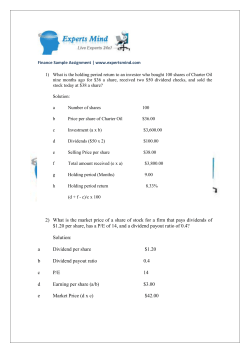


© Copyright 2026