1. No category

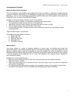
Two Sample t Test and its Applications
Data Analysis II
1. Introduction
The two sample t-test is used to compare two groups. This test has some variations
depending on whether these two groups are independent, paired, or both, whether the
sample size is large enough, and on whether the sample meets certain assumptions.
Although according to the Central Limit Theorem, large enough samples would have
normally distributed sample means regardless of the population distributions the samples
came from, and large enough is usually greater than 30, it is always safer to test the data
in case it might need some transformations; especially since various computer programs
make testing for normality relatively simple.
If assumptions for the t-test are not met, the corresponding nonparametric tests should be
used. Nonparametric test also have assumptions, but these are less rigorous than the
parametric tests.
In some situations one might use independent where paired was most appropriate or vice
versa. It is important to use the right test since each would give the best results when
properly used.
The different t test can be performed with the aid statistical packages such as Sas and
Spss preferably, but if not available Microsoft Excel can also be used.
Independent or Paired
Independent refers to non correlated groups, while paired refers to two different
treatments on the same group.
Independent
Examples of independent groups will be testing the gpa of males versus females;
consumer’s preference on some brand versus another; one method or production versus
another.
Basically independent test is for comparing between two independent groups as the name
suggests.
Paired
Examples of experiments on paired groups would be comparing test performance of
students before and after a tutoring program; amount of some body fluid before and after
some treatment; operation of some system before and after a change.
Although in general paired test is for some before and after type of situation on the same
subject, we can present some examples of pairs without using the same subject. For
example: comparing some aspect using twins, married couples, or any two closely
related subjects. These examples would be better described as matched pairs.
Note that paired samples have less variability than independent samples. A paired test is
the same as a single t test on the differences of the two samples.
Assumptions
Once paired or independent has been selected, the next step will be to check for
assumptions. Some alternative procedure exist in cases were assumptions for a
particular test are not met. Using the wrong test or not checking assumptions would give
invalid results.
Independent t-test Assumptions
The two samples are randomly and independently selected from the two populations.
The two populations are normally distributed.
The two sample variances are equal.
Note: For large samples (n1 and n2 ≥ 30) the sample variances do not have to be equal.
For small samples (n1 or n2 or both ≤ 30) there is an alternative test when variances
cannot be assumed equal. The F test checks the equal variance assumption.
Paired t-test Assumptions
Since the observations are paired in this case we test the differences.
The population of differences has a normal distribution.
The differences are independent.
The differences have equal mean and variance.
Bar charts in Excel and/or Q-Q plots and the Kolmogorov-Smirnov test in statistical
packages will check the normality data assumption. If the data does not follow a normal
distribution transformations can be done. For example the log transformation usually
works for right skewed data. If the log produces a normal transformation then the data is
called lognormal. Reciprocal and square root transformations are also performed
depending on what the original data looks like.
Transformed data will lose some information. The final result could be changed back to
the original scale but rather than interpreting the differences in means it the results would
express the ratio of the means.
Statistical packages as well as Excel will also check for equal variances. Statistical
packages will show two results: one for equal variances assumed and one for equal
variances not assumed. Excel uses the F-test to check for equal variances and then one
can choose from the t test for equal variances or the t test for not equal variances
depending of course on the result obtained from the F-test.
If the data does not follow a normal distribution then a corresponding nonparametric test
would have to be used.
Nonparametric tests
Note: Nonparametric tests use the median and/or ranks rather than the mean and have
fewer restrictions than parametric tests.
For Independent samples: Mann-Whitney
Assumptions
The samples are random and independent each from populations with unknown medians.
Continuous variable measured on at least an ordinal scale.
The distributions differ only with respect to location.
For Paired samples: Wilcoxon Matched-Pairs Signed-Ranks
Assumptions
The differences come from random samples of matched continuous variables.
The differences are independent, and measured on at least an interval scale.
The distribution of differences is symmetric about the median.
Note: Although not as popular as the above tests, the Median test for independent
samples and the Sign test for paired samples are also nonparametric tests available.
2. Methodology
Independent Samples
Hypotheses
A. Ho: µ1 - µ2 = δ0
B. Ho: µ1- µ2 ≥ δ0
C. Ho: µ1- µ2 ≤ δ0
Ha: µ1- µ2 ≠ δ0
Ha: µ1- µ2 < δ0
Ha: µ1- µ2 > δ0
Large sample size: n1 and n2 ≥ 30
Test Statistic
z=
( x1 − x 2 ) − δ 0
σ 12
n1
+
σ 22
n2
Rejection Region
A. Reject Ho if |z| > zα/2
B. Reject Ho if z < -zα
C. Reject Ho if z > zα
100(1- α)% Confidence Interval
A. ( x 1 − x 2 ) ± zα / 2
σ 12
n1
+
σ 22
n2
B. ( µ1 − µ 2 ) ≤ ( x1 − x 2 ) + zα
C. ( µ1 − µ 2 ) ≥ ( x1 − x 2 ) − zα
σ 12
n1
σ 12
n1
+
+
σ 22
n2
σ 22
n2
Small samples n1 or n2 or both ≤ 30
Equal variances assumed
σ1 = σ2
The F tests checks for equal variances
Ho: σ 12 = σ 22
Ha: σ 12 ≠ σ 22
s12
s 22
F=
Reject Ho if F > f n1 −1,n2 −1,α / 2 or F < f n1 −1,n2 −1, −α / 2
Test Statistic
t=
( x1 − x 2 ) − δ 0
SP
1
1
+
n1 n 2
where S P stands for pooled variance and
(n1 − 1) s12 + (n2 − 1) s 22
S =
n1 + n2 − 2
2
P
Rejection Region
A. Reject Ho if |t| > tv,α/2
B. Reject Ho if t < -tv,α
C. Reject Ho if t > tv,α
Where v stands for degrees of freedom and v = n1+ n2 - 2
100(1- α)% Confidence Interval
A. ( x 1 − x 2 ) ± t v ,α / 2 S P
1
1
+
n1 n 2
B. ( µ1 − µ 2 ) ≤ ( x1 − x 2 ) + t v ,α S P
1
1
+
n1 n2
C. ( µ1 − µ 2 ) ≥ ( x1 − x 2 ) − t v ,α S P
1
1
+
n1 n2
Equal variances not assumed
σ1 ≠ σ2
Test Statistic
t=
( x1 − x 2 ) − δ 0
s12 s 22
+
n1 n2
Rejection Region
A. Reject Ho if |t| > tv,α/2
B. Reject Ho if t < -tv,α
C. Reject Ho if t > tv,α
Where v stands for degrees of freedom and
( w1 + w2 ) 2
v= 2
,
w1 /(n1 − 1) + w22 /(n2 − 1)
s12
w1 =
,
n1
s 22
w2 =
n2
100(1- α)% Confidence Interval
A. ( x 1 − x 2 ) ± t v ,α / 2
s12 s 22
+
n1 n2
B. ( µ1 − µ 2 ) ≤ ( x1 − x 2 ) + t v ,α
s12 s 22
+
n1 n2
C. ( µ1 − µ 2 ) ≥ ( x1 − x 2 ) − t v ,α
s12 s 22
+
n1 n2
Paired Samples
Hypotheses
A. Ho: µd = δ0
B. Ho: µd ≥ δ0
C. Ho: µd ≤ δ0
Ha: µd ≠ δ0
Ha: µd < δ0
Ha: µd > δ0
µd = µ1- µ2
Large sample
Test Statistic
z=
xd − δ0
σ d / nd
where x d = sample mean differences
σ d or sd = standard deviation of differences
nd = number of differences (pairs)
Rejection Region
A. Reject Ho if |z| > zα/2
B. Reject Ho if z < -zα
C. Reject Ho if z > zα
100(1- α)% Confidence Interval
A. x d ± zα / 2
σd
σ d ≈ sd
nd
σd
B. µ d ≤ x d + zα
nd
σd
C. µ d ≥ x d − zα
nd
Small samples
Test Statistic
t=
xd − δ0
s d / nd
Rejection Region
A. Reject Ho if |t| > t nd −1,α / 2
B. Reject Ho if t < - t nd −1,α
C. Reject Ho if t > t nd −1,α
100(1- α)% Confidence Interval
A. x d ± t nd −1,α / 2
sd
nd
B. µ d ≤ x d + t nd −1,α
sd
C. µ d ≥ x d − t nd −1,α
sd
nd
nd
Note: Paper 3 suggests a corrected z test for samples with combined independent and
paired observations explaining how this test will give more accurate results than either of
the above tests.
3. Applications
Independent Samples
Equal Variances
This example was taken from http://bmj.bmjjournals.com/collections/statsbk/7.shtml
The addition of bran to the diet has been reported to benefit patients with diverticulosis.
Several different bran preparations are available, and a clinician wants to test the efficacy
of two of them on patients, since favorable claims have been made for each. Among the
consequences of administering bran that requires testing is the transit time through the
alimentary canal. Does it differ in the two groups of patients taking these two
preparations?
The null hypothesis is that the two groups come from the same population. By random
allocation the clinician selects two groups of patients aged 40-64 with diverticulosis of
comparable severity. Sample 1 contains 15 patients who are given treatment A, and
sample 2 contains 12 patients who are given treatment B. The transit times of food
through the gut are measured by a standard technique with marked pellets and the results
are recorded, in order of increasing time, in Table 7.1 .
These data are shown in figure 7.1 . The assumption of approximate Normality and
equality of variance are satisfied. The design suggests that the observations are indeed
independent. Since it is possible for the difference in mean transit times for A-B to be
positive or negative, we will employ a two sided test.
With treatment A the mean transit time was 68.40 h and with treatment B 83.42 h. What
is the significance of the difference, 15.02h?
The table of the tdistribution Table B (appendix) which gives two sided P values is
entered at
degrees of freedom.
For the transit times of table 7.1,
Treatment A Treatment B
shows that
at 25 degrees of freedom (that is (15 - 1) + (12 - 1)), t= 2.282 lies between 2.060 and
2.485. Consequently,
. This degree of probability is smaller than the
conventional level of 5%. The null hypothesis that there is no difference between the
means is therefore somewhat unlikely.
A 95% confidence interval is given by
83.42 - 68.40 2.06 x 6.582
15.02 - 13.56 to 15.02 + 13.56 or 1.46 to 18.58 h.
Unequal standard deviations
If the standard deviations in the two groups are markedly different, for example if the
ratio of the larger to the smaller is greater than two, then one of the assumptions of the
ttest (that the two samples come from populations with the same standard deviation) is
unlikely to hold.
The unequal variance t test tends to be less powerful than the usual t test if the variances
are in fact the same, since it uses fewer assumptions. However, it should not be used
indiscriminantly because, if the standard deviations are different, how can we interpret a
nonsignificant difference in means, for example? Often a better strategy is to try a data
transformation, such as taking logarithms as described in Chapter 2. Transformations that
render distributions closer to Normality often also make the standard deviations similar.
If a log transformation is successful use the usual t test on the logged data.
Applying this method to the data of Table 7.1
Thus d.f. = 22.9, or approximately 23. The tabulated values for 2% and 5% from table B
are 2.069 and 2.500, and so this gives
as before. This might be expected,
because the standard deviations in the original data set are very similar and the sample
sizes are close, and so using the unequal variances t test gives very similar results to the
t test which assumes equal variances.
Unequal Variances
This Example was taken from
http://www.people.vcu.edu/~wsstreet/courses/314_20033/hyptest2ex.pdf
2. Two sections of a class in statistics were taught by two different methods. Students’
scores on a standardized test are shown below. Do the results present evidence of a
difference in the effectiveness of the two methods? (Use á = 0.01.)
Step 1 : Hypotheses
H0 : µA - µB = 0
Ha: µA - µB = 0
Step 2 : Significance Level
α= 0.01
Step 3 : Critical Value(s) and Rejection Region(s)
Since we don’t know the population variances and don’t think that they are equal, we’ll
use the non-pooled t-test.
Reject the null hypothesis if T_≤_–2.82 or if T ≥ 2.82.
Step 4 : Test Statistic
T = 1.2193
p - value = 0.242
Step 5 : Conclusion
Since –2.82 ≤ 1.2193 ≤ 2.82 ( p-value ≈ 0.242 > 0.01), we fail to reject
the null hypothesis.
Step 6 : State conclusion in words
At the α = 0.01 level of significance, there is not enough evidence to conclude
that there is a difference in the effectiveness of the two methods.
Paired Samples
This example was taken from http://www.physics.csbsju.edu/stats/t-test.html
Cedar-apple rust is a (non-fatal) disease that affects apple trees. Its most obvious
symptom is rust-colored spots on apple leaves. Red cedar trees are the immediate source
of the fungus that infects the apple trees. If you could remove all red cedar trees within a
few miles of the orchard, you should eliminate the problem. In the first year of this
experiment the number of affected leaves on 8 trees was counted; the following winter all
red cedar trees within 100 yards of the orchard were removed and the following year the
same trees were examined for affected leaves. The results are recorded below:
tree
number of rusted
leaves: year 1
number of rusted
leaves: year 2
1
2
3
4
5
6
7
8
38
10
84
36
50
35
73
48
32
16
57
28
55
12
61
29
6
-6
27
8
-5
23
12
19
46.8
23
36.2
19
10.5
12
average
standard dev
difference: 1-2
As you can see there is substantial natural variation in the number of affected leaves; in
fact, an unpaired t-test comparing the results in year 1 and year 2 would find no
significant difference. (Note that an unpaired t-test should not be applied to this data
because the second sample was not in fact randomly selected.) However, if we focus on
the difference we find that the average difference is significantly different from zero. The
paired t-test focuses on the difference between the paired data and reports the probability
that the actual mean difference is consistent with zero. This comparison is aided by the
reduction in variance achieved by taking the differences.
4. Discussion
Since the t test has variations according to the above explained situations, one must
carefully decide whether the samples are independent or paired (or even samples
combined of both independent and paired observations) and whether the required
assumptions for the particular chosen test hold to avoid obtaining invalid results.
A test for paired samples reduces to a single t test performed on the differences.
Independent samples t test has more power when the respective variances can be assumed
equal (by testing them with the F test first.) Paired experiments are preferable since less
variation exits, however if the samples are independent the t test for paired would give
invalid results (and vice versa.)
Sometimes a sample could contain a combination of paired and independent
observations. In this case a corrected z test (as explained in “Paper 3”) should be
employed.
References
1. Papers 1-4
2. Tamhane, Ajit C. and. Dunlop, Dorothy D (2000). Statistics and Data Analysis from
Elementary to Intermediate, Upper Saddle River: Prentice Hall, Inc.
3. Daniel, Wayne W. (1990). Applied Nonparametric Statistics, Second Edition, Boston:
PWS-Kent Publishing Company.
4. http://www.physics.csbsju.edu/stats/t-test.html
5. http://www.people.vcu.edu/~wsstreet/courses/314_20033/hyptest2ex.pdf
6. http://bmj.bmjjournals.com/collections/statsbk/7.shtml