EE235
Univ. of Washington
Sample Final Exam (from another quarter)
• The test is closed book and no calculators/devices are allowed. You are allowed TWO
8.5×11 (two-sided) page of notes.
• Please show all work. Partial credit will be given to partial work.
• There are 8 problems with 62 total points. Please use your blue book for solutions.
• Please observe the honor code.
π
1. (5 pts) Consider an LTI systems with transfer function H(ω) = 21 e−j 3 ω .
(a) (1 pt) Sketch magnitude of H(ω).
|H(ω)|
0.5
ω
1
(b) (1 pt) Sketch the phase of H(ω).
∠H(ω)
π/3
ω
−1
1
−π/3
(c) (1 pt) Find the impulse response h(t).
Use the transform
F
δ(t − t0 ) −→ e−jwt0
with t0 =
π
3
and by linearity,
1
π
1 jwπ
F
h(t) = δ(t − ) −→ e− 3
2
3
2
1
(d) (1 pt) Is the system causal? (just yes or no)
Yes – h(t) is a causal signal.
(e) (1 pt) Is this system best described as a lowpass, bandpass, highpass, or allpass
system?
Allpass from the magnitude graph of (a)
2. (5 pts) Using the properties of the Fourier transform, find the time domain signal y(t). (?
denotes convolution)
y(t) = sinc(t) ? ej5t sinc(t)
Use the transform pair
F
f (t) = sinc(t) −→ F (ω) = π rect(ω/2)
with the frequency shift property
F
eω0 t −→ F (ω − ω0 )
and the linearity property of Fourier transforms to get
F
g(t) = ej5t sinc(t) −→ G(ω) = π rect(
ω−5
).
2
Convolution in time corresponds to multiplication in frequency domain
F
y(t) = f (t) ? g(t) −→ Y (ω) = F (ω)G(ω)
Plotting F (ω) and G(ω) rects,
F (ω)
G(ω)
π
ω
−1
1
4
5
6
since the two rect functions don’t have an overlap, the product is zero everywhere: Y (ω) =
0 and therefore y(t) = 0 .
3. (4 pts) You are given the pole-zero plot of an LTI transfer function H(s) below, and you’re
told that the system is causal.
2 jω
σ
−1
−2
2
(a) (1 pt) What is the ROC?
The system is causal so the ROC is Re{s} > −1 .
(b) (1 pt) Is the system stable?
Yes, since the system is causal and all poles are in the left half plane (alternatively,
it’s stable since the ROC includes the jω axis).
(c) (2 pt) Based on the pole-zero locations, which of the following signals can be the
impulse response of the system? What is ω0 ? (no need to find constants A, B, φ).
ha (t) = A cos(ω0 t + φ)u(t) + Be−t u(t)
hb (t) = e−t [A cos(ω0 t + φ) + B]u(t)
Signal a cannot have the given pole-zero plot because the poles for cos(ω0 t + φ)u(t)
must be on the jw-axis (the poles are at s = ±jω0 )
Signal b can have the poles at s = −1 ± 2j since the complex poles of the decaying
cosine are at s = −1 ± jω0 (the e−t shifts the poles of the cosine by −1).
ω0 = 2
4. (10 pts) Let
x(t) = sin(2t) cos(t) − e−j3t + 2
(a) (2 pts) What is the period of x(t)?
Use the trig identity 2 sin(x) cos(y) = sin(x − y) + sin(x + y),
x(t) =
1
1
sin(t) + sin(3t) − e−j3t + 2
2
2
The fundamental frequency is ω0 = GCD(1, 3, 3) = 1 and the period is
T =
2π 2π
2π
= LCM (2π, , ) = 2π .
ω0
3 3
(b) (4 pts) P
Find the exponential Fourier series coefficients of x(t) (i.e., find dk in
jkω0 t . The coefficients d don’t need to be simplified.)
x(t) = ∞
k
−∞ dk e
Use Euler’s to convert the sines to complex exponentials
x(t) =
1 1 j3t
1 1 jt
[e − e−jt ] +
[e − e−j3t ] − e−j3t + 2
2 2j
2 2j
Rearranging terms,
x(t) = 2 +
1 jt
1
1
1
e − e−jt + ej3t − (1 + )e−j3t
4j
4j
4j
4j
Since ω0 = 1
x(t) = 2ejω0 0 +
1 jω0 t
1
1
1
e
− e−jω0 t + ej3ω0 t − (1 + )e−j3ω0 t
4j
4j
4j
4j
3
So the Fourier series coefficients are:
d0 = 2 d1 =
1
4j
d−1 = −
1
4j
d3 =
1
4j
d−3 = −(1 +
1
)
4j
(c) (4 pts) If x(t) given above is the input to an LTI system with impulse response
sin(2t)
,
t
find the output of the system, y(t). Simplify your y(t) so it does not have any j’s in
it (it’s a real signal). Hint: First sketch H(ω).
Rewrite the impulse response as a sinc,
h(t) =
h(t) =
sin(2t)
sin(2t)
=2
= 2 sinc(2t)
t
2t
so the transfer function is
H(ω) = πrect(ω/4)
H(ω) is an ideal lowpass filter with bandwidth ω = −2 to ω = 2 and a gain of π.
Only frequencies ω = ±1 and ω = 0 pass through the filter and are multiplied by π,
so the output is
y(t) = π sin(t) + 2π
5. (6 pts) For each of the systems below, can you tell whether it CAN or CANNOT be LTI?
Give a one line explanation for your answer (no credit for correct answer without any
explanation).
Solution Note: We know that complex exponentials est are the eigenfunctions of LTI
systems and the output to them will be of the form H(s)est . This means an LTI systems
cannot change the frequency content of its input signal. So we can write the input and
the output in terms of est where s is a complex number, and check whether the output
includes any new frequencies.
Note that since we’re given only one input-output pair, we cannot test linearity and time
invariance directly.
(a) (2 pts) For the input x(t) = 1 + cos(t + 5) the output is y(t) = 2 + ej(t+1) .
CAN be LTI: An LTI system cannot create new frequencies (since ejw0 t is an eigenfunction for an LTI system, the output corresponding to an input with frequency w0
has the same frequency w0 .)
Decompose the input and output into a sum of complex exponential signals
x(t) = 1 + 0.5ej(t+5) + 0.5e−j(t+5)
= 1 + 0.5ej5 ejt + 0.5e−j5 e−jt
y(t) = 2 + e · ejt + 0 · e−jt .
Since input has ej0t , ejt , e−jt terms, and the output has the same terms (no new
frequencies), the system could be LTI.
4
(b) (2 pts) For an input x(t) = cos(3t) the output is y(t) = e−3t cos(3t).
CANNOT be LTI: Decompose the input and output into a sum of complex exponential signals
x(t) = 0.5ej3t + 0.5e−j3t
y(t) = e−3t [0.5ej3t + 0.5e−j3t ]
= 0.5e(3+j3)t + 0.5e(3−j3)t
Since input has frequencies 3j and −3j, but the output has new frequencies, 3 + j3
and 3 − j3, so the system cannot be LTI.
(c) (2 pts) The Fourier transforms of the input x(t) and output y(t) are given below.
Y (ω)
X(ω)
ω
ω
π
−π
−2π
2π
CANNOT be LTI: The output has a larger bandwidth than the input (new frequencies have been added).
6. (16 pts)
(a) (1 pt) If a periodic signal has Fourier series coefficients dk , what is its Fourier transform? (write the Fourier transform in terms of dk ).
The formula for a Fourier series with period T and fundamental frequency w0 = 2π/T
is
∞
X
f (t) =
dk ejkw0 t
k=−∞
Noting that the Fourier transform pair
F
ejat −→ 2πδ(w − a)
with a = kw0 and invoking linearity, we get
f (t) =
∞
X
F
dk ejkw0 t −→ F (w) =
k=−∞
∞
X
2πdk δ(w − kw0 )
k=−∞
(b) (2 pts) Consider the periodic signal
m(t) =
∞
X
δ(t − 2k) − δ(t − (2k + 1)).
k=−∞
Sketch m(t). What is the its period?
5
1
m(t)
t
−3
−2
−1
1
2
3
−1
The period is T = 2
(c) (4 pts) Compute its Fourier series coefficients dk , and show that dk = 0 for even k,
and dk = 1 for odd k.
We need to look at m(t) over one period, say −0.5 to 1.5, to get δ(t) − δ(t − 1). Note
that ω0 = π. Then
Z
1
dk =
f (t)e−jω0 t dt
T T
Z
1 1.5
(δ(t) − δ(t − 1))e−jπt dt
=
2 −0.5
Z 1.5
Z
1 1.5
1
=
δ(t − 1)
δ(t) − e−jkπ
2 −0.5
2
−0.5
1
= (1 − e−jkπ )
2
1
= (1 − (−1)k )
2
which is 0 for k even, and 1 for k odd.
(d) (2 pts) Sketch M (ω), the Fourier transform of m(t) (label your axes clearly).
1
M (ω)
ω
−3π −2π −1π
1π
2π
3π
(e) (4 pts) Consider a signal x(t) that is bandlimited to ω ∈ [−B, B] (as shown in the
figure).
X(ω)
ω
-B
B
If we ‘sample’ x(t) by multiplying it with m(t), what is the largest value of B for
which there is no aliasing?
We should have 2B < 2π =⇒ B < π, to avoid aliasing.
Sketch the Fourier transform of xs (t) = x(t)m(t).
For x(t) is sampled at the Nyquist frequency, so B = π,
6
Xs (ω)
ω
−4π −3π −2π −1π
1π
2π
3π
4π
(f) (2 pts) We can recover the original signal x(t) by forming xs (t) cos(ωr t) and then
applying an ideal low-pass filter. What is ωr ?
ωr = ω0 = π to shift a copy of X(ω) so that it’s centered at zero and picked out by
an ideal low-pass filter.
F{xs (t) cos(πt)}
ω
−4π −3π −2π −1π
1π
2π
3π
4π
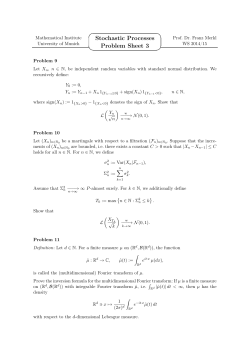
7. (9 pts) Let X(ω) denote the Fourier transform of the signal x(t) shown in the figure.
x(t)
2
1
t
−3
−2
−1
1
2
3
Using the properties of the Fourier transform,
(a) (2 pts) Find X(0).
Setting ω = 0 in the definition of the Fourier transform,
Z ∞
X(w) =
x(t)e−jwt dt
−∞
Z ∞
X(0) = X(w)w=0 =
x(t)e−j0t dt
−∞
Z ∞
=
x(t)dt
−∞
so X(0) is the area under x(t). From the figure this is the sum of the areas of a
rectangle and a half-circle, 2 + π/2 .
7
R∞
(b) (2 pts) Find −∞ X(ω)dω.
Setting t = 0 in the inverse Fourier transform formula,
Z ∞
1
X(ω)ejwt dω
x(t) =
2π −∞
Z ∞
1
x(0) = x(t)t=0 =
X(ω)ejw0 dω
2π −∞
Z ∞
1
X(ω)dω
=
2π −∞
Z ∞
2πx(0) =
X(ω)dω
−∞
R∞
−∞ X(ω)dω = 2πx(0)
R∞
Find −∞ e−j2ω X(ω)dω.
so we get
= 4π .
(c) (2 pts)
Setting t = −2 we get
1
2π
Z
∞
X(ω)ejwt dω
−∞
Z ∞
1
X(ω)e−j2w dω
x(−2) = x(t) t=−2 =
2π −∞
Z ∞
2πx(−2) =
X(ω)e−j2w dω
x(t) =
−∞
R∞
(d)
−j2ω X(ω)dω = 2πx(−2)
−∞ e
R∞
(3 pts) Find −∞ ωX(ω)dω.
= 0.
G(ω) = ωX(ω) is the Fourier transform of g(t) = 1j dx(t)
dt , so its integral is the value
of
g
at
t
=
0.
From
the
figure
dx(t)/dt
which
is
the
slope
of x(t) at t = 0 is zero, so
R∞
−∞ ωX(ω)dω = 0 .
You could also have noted that since x(t) is real, then X(w) = X ∗ (−w) so Re(X(w))
is even and Im(X(w)) is odd. Therefore, Re(wX(w)) is odd and Im(wX(w)) is odd,
so
Z ∞
Z ∞
ωX(ω)dω =
[Re(wX(w)) + Im(wX(w))]dω = 0
−∞
−∞
8