
Aerodynamic Shape Optimization Part II: Sample Applications
Aerodynamic Shape Optimization Part II: Sample Applications John C. Vassberg ∗ Phantom Works The Boeing Company Huntington Beach, CA 92647-2099, USA Antony Jameson † Department of Aeronautics and Astronautics Stanford University Stanford, CA 94305-3030, USA Von Karman Institue Brussels, Belgium 9 March, 2006 Nomenclature A AR b B CF D CD CL Cref count F G H HP I KEAS MP H N R RAN S RCS Re Reθ Sref U AV x q w λ Λc/4 ∞ δ∗ O(∗) (∗)−1 Hessian Matrix / Operator 2 Wing Aspect Ratio = Sbref Wing Span Shape Function Basis Computational Fluid Dynamics Drag Drag Coefficient = q∞ Sref t Lift Coefficient = q∞Lif Sref Wing Reference Chord Drag Coefficient Unit = 0.0001 Surface Defining Function Gradient of Cost Function Estimate of Inverse Hessian Matrix Horse Power Objective or Cost Function Knots Equivalent Air Speed Mile Per Hour Number of Design Variables Flow-Equation Function Reynolds-Averaged Navier-Stokes Reaction Control System Wing Reynolds number based on Cref Attachment Line Reynolds number Wing Reference Area Unmanned Aerial Vehicle Independent Spatial Variable Dynamic Pressure = 12 ρV 2 Flow Variable Wing Taper Ratio; Search Step Parameter Wing Quarter-Chord Sweep Infinity First Variation of Order of Inverse Matrix of ∗ Boeing † T. Technical Fellow V. Jones Prof. of Engineering c 2006 by Vassberg & Jameson. Copyright Published by the VKI with permission. 1 Introduction This is the second of two lectures prepared by the authors for the von Karman Institute that deal with the subject of aerodynamic shape optimization. In our first lecture we introduced some theoretical background on optimization techniques commonly used in the industry, applied these approaches to a couple of very simple model problems, compared the results of these schemes, and discussed their merits and defficiencies as they relate to the class of aerodynamic shape optimization problems the authors deal with on a regular basis. In this lecture, we illustrate how the gradient of a complex system of nonlinear partial differerential equations can be obtained for about the same computational cost as that of the cost function, and we provide a set of sample applications. In an airplane design environment, there is no need for an optimization based purely on the aerodynamics of the aircraft. The driving force behind (almost) every design change is related to how the modification improves the vehicle, not how it enhances any one of the many disciplines that comprise the design. Although we focus this lecture on the aerodynamics of an airplane, we also include the means by which other disciplines are linked into and affect the aerodynamic shape optimization subtask. Another characteristic of the problems we typically (but not always) work on is that the baseline configuration is itself within 1-2% of what may be possible, given the set of constraints that we are asked to satisfy. This is certainly true for commercial transport jet aircraft whose designs have been constantly evolving for the past half century or more. The sample applications provided herein do not fall into this category. Quite often the problem can be very constrained; this is the case when the shape change is required to be a retrofitable modification that can be applied to air- Vassberg & Jameson, VKI Lecture-II, Brussels, Belgium, 9 March, 2006 1 of 41 craft already in service. Occasionally, we can begin with a clean slate, such as in the design of an all-new airplane. And the problems cover the full spectrum of studies in between these two extremes. Let’s note a couple of items about this setting. First, in order to realize a true improvement to the baseline configuration, a high-fidelity and very accurate computational fluid dynamics (CFD) method must be employed to provide the aerodynamic metrics of lift, drag, pitching moment, spanload, etc. Even with this, measures should be taken to estimate the possible error band of the final analyses; this discussion is beyond the scope of these lectures. Figures 1-2 illustrate the class of aircraft and the level of detail the first author addresses every day. These Navier-Stokes CFD solutions are conducted on fullup cruise configurations, complete with wing, fuselage, engine groups, empennage, flap-support fairings, and winglets. The engine groups include a pylon, nacelle, core-cowl, shelf, and bifurcation flows. Although not obvious in these images, various fillets are also included. Finally, the CFD calculations are performed at prescribed lifting conditions by altering angle-of-attack, and are trimmed to specified centerof-gravity locations by adjusting the horizontal tail incidence. This level of detail is needed to achieve an accuracy on the absolute performance of the aircraft that is within 1% of flight test data. However, this is what is required to improve the performance of the aircraft by 1-2% without a numerical optimization yielding a false positive. The second item to consider is related to the definition of the design space. A common practice is to use a set of basis functions which either describe the absolute shape of the geometry, or define a perturbation relative to the baseline configuration. In order to realize an improvement to the baseline shape, the design space should not be artificially constrained by the choice of the set of basis functions. This can be accomplished with either a small set of very-well-chosen basis functions, or with a large set of reasonably-chosen basis functions. The former approach places the burden on the user to establish an adequate design space, the later approach places the burden on the optimization software to economically accommodate problems with large degrees of freedom. Over the past decade, the authors have focused on solving the problem of aerodynamic shape optimization utilizing a design space of very large dimension. Our principal motivation for addressing the problem of large number of design variables is two fold. The first is to provide a situation where the design space never needs to be artificially constrained. The second is to allow us the flexibility to automatically set up the design space within the optimization software at the highest dimensionality supported by the discrete numerical simulation. In doing so, the aerodynamic shape optimization software based on these concepts allow the user to run optimizations immediately after set up of the analysis inputs are complete. This speeds time-to-firstoptimization and minimizes the human errors associated with defining a design space. Furthermore, aerodynamic shape optimizations based on either the Euler or Navier-Stokes equations can be run on relatively inexpensive computer equipment. The next section provides an overview of aerodynamic optimization. We develop an efficient evaluation for the gradient; this is based on solving an adjoint equation. A brief review of the search methods we utilize are then included. Following this discussion, we present a few selected case studies. These sample applications are all on design activities that we have been involved with; they include a Mars aircraft, a Reno Racer, and an aero-structural optimization of a generic B747 wing/body configuration. 2 Aerodynamic Design Trades The objective of aerodynamic design is to produce a structurally feasible shape with sufficient carrying capacity, which achieves good aerodynamic performance. For example, consider the generic task of delivering a payload between distant city pairs. The Breguet Range equation, which aptly applies to long-range missions of jet aircraft, is: W0 + Wf ML a . (1) ln Range = D SF C W0 Here, M is the cruise Mach number, L & D are the aerodynamic forces of lift and drag, respectively, a is the acoustic speed, SF C is the specific fuel consumption of the engines, W0 is the aircraft landing weight, and Wf is the weight of fuel burned during the flight. The Breguet Range equation illustrates the importance of drag prediction as a function of lift and Mach number in the context of aerodynamic design; it also provides a glimpse into the interplay between the various disciplines. Referring to Eqn (1), one might assume that the aerodynamic efficiency of an aircraft is represented by ML D , the propulsion efficiency is embedded in SF C, and that the structural efficiency directly impacts W0 . Interestingly, historical trends of inservice transport aircraft indicate that very little improvement in the ML D metric has been accomplished in the past 40 years. Yet it would be somewhat naive to state that no aerodynamic advances have been made during this period. In actuality, advances in aerodynamics have better served aircraft designs when traded for improvements in other disciplines. Vassberg & Jameson, VKI Lecture-II, Brussels, Belgium, 9 March, 2006 2 of 41 For example, the ability to increase the thickness-tochord ratio of a wing while maintaining ML D not only reduces the structural weight of the wing, it also provides additional fuel volume. In terms of Eqn (1), an aerodynamic improvement of this nature would manifest itself as a decrease in W0 and an increase in Wf with the net result being an increase in range. Reducing the aircraft’s empty weight has the added benefit of reducing the cost of the vehicle. Obviously, this aerodynamic improvement would not be apparent in the trend charts of ML D . Assume that an airline would like to provide a service between two cities with an aircraft that, when fully loaded with payload and fuel, is 1% short on range. Since the aircraft is fuel-volume limited, the only recourse is to reduce the payload weight. In relative terms, a typical ratio of weights might have Wf = 23 W0 and Wpayload = 61 W0 . In this scenario, Eqn (1) shows that the operator would have to reduce the payload (read revenue) by 7.6% to recover the 1% shortfall on range. Since most airlines operate on very small margins, this service most likely will no longer be a profit-generating venture. This example illustrates that in the current business of flight, a 1% delta in aircraft performance is a significant change. While improving an aircraft’s performance by 1% may not be a trivial task given the usual constraints, losing 5% is easily done if attention is not paid to details such as juncture flows, external doublers, gaps, etc. Now consider a more typical case where the aircraft does not suffer from a shortfall on range. In round numbers, the Direct Operating Costs (DOC) of a transport aircraft can be itemized as: 50% for the cost of ownership, 20% for fuel burn, 20% for crew salaries and maintanence, and 10% for miscellaneous other items. From an airline’s perspective, if the DOC of its fleet of aircraft could be reduced by 5% with a new design (while providing the same set of services to its customers), the airline would most likely retire its entire fleet and replace it with the new aircraft [1]. So how can aerodynamics be leveraged to improve the economics associated with a flight-based mission? By enabling the development of a simplified high-liftL and CL max reduces system design that for a given D manufacturing and maintanence costs as well as part count. By increasing the cruise Mach number without reducing ML D reduces the time-dependent costs such as crew and maintanence. Also, by increasing ML D without penalizing the other disciplines reduces fuel burn. These are just a few examples that illustrate how aerodynamic advances would impact on DOC. A common requirement for achieving these goals is the accurate prediction of drag. To push aerodynamic technologies forward, it is becoming more important that accurate drag prediction become a consistent product of the CFD community. Once this prerequisite is accomplished, the full benefits of automated aerodynamic shape optimization may begin to be realized. With the various on-going design programs, these are exciting times for the aircraft industry. A prime example is the Blended-Wing-Body (BWB) which has established a renaissance in the design of a family of all-new aircraft [2]. This revolutionary concept is enabling aerodynamic advances in all of the above areas, and then some. It presents challenges, yet offers significant opportunities, and as a result, a 5% reduction in DOC is within grasp. Suffice it to say that aerodynamics is not a sunset technology, but rather, it is as important today as it was a century ago; only the stakes have changed. 3 Aerodynamic Optimization Traditionally the process of selecting design variations has been carried out by trial and error, relying on the intuition and experience of the designer. The degree of success with this classical approach depends directly on the level of expertise of the aerodynamic designer, which can take over a decade of apprenticeship to develop. It is not at all likely that a similar process of repeated trials in an interactive design and analysis procedure can lead to a truly optimum design. In order to take full advantage of the possibility of examining a large design space, the numerical simulations need to be combined with automatic search and optimization procedures. This can lead to automatic design methods which will fully realize the potential improvements in aerodynamic efficiency. An approach which has become increasingly popular is to carry out a search over a large number of variations via a genetic algorithm. This may allow the discovery of (sometimes unexpected) optimum design choices in very complex multi-objective problems, but it becomes extremely expensive when each evaluation of the cost function requires intensive computation, as is the case in aerodynamic problems. In order to find optimum aerodynamic shapes with reasonable computational costs, it pays to embed the flow physics within the optimization process. In fact, one may regard an aerodynamic shape as a device to control the flow in order to produce a specified lift with minimum drag. As a result, one can draw on concepts which have been developed in the mathematical theory of control of systems governed by partial differential equations. In particular, an acceptable aerodynamic design must have characteristics that do not abruptly vary with small changes in Vassberg & Jameson, VKI Lecture-II, Brussels, Belgium, 9 March, 2006 3 of 41 shape and flow conditions. Consequently, gradientbased procedures are appropriate for aerodynamic shape optimization. Two main issues affect the efficiency of gradient-based procedures; the first is the actual calculation of the gradient, and the second is the construction of an efficient search procedure which utilizes the gradient. 3.1 Gradient Calculation For the class of aerodynamic optimization problems under consideration, the design space is essentially infinitely dimensional. Suppose that the performance of a system design can be measured by a cost function I which depends on a function F(x) that describes the shape, where under a variation of the design, δF(x), the variation of the cost is δI. Now suppose that δI can be expressed to first order as Z δI = G(x)δF(x)dx to estimate the gradient is proportional to the number of design variables [3]. Similarly, if one resorts to direct code differentiation (ADIFOR [4, 5]), or complex-variable perturbations [6], the cost of determining the gradient is also directly proportional to the number of variables used to define the design. Even small problems of aerodynamic shape optimization based on these approaches can require compute resources that are measured in CPU-Years, which can only be completed in reasonable elapsed time through utilization of massively-parallel computers costing millions of dollars. A more cost effective technique is to compute the gradient through the solution of an adjoint problem, such as that developed in [7, 8, 9]. The essential idea may be summarized as follows. For flow about an arbitrary body, the aerodynamic properties that define the cost function are functions of the flowfield variables (w) and the physical shape of the body, which may be represented by the function F. Then I = I(w, F) where G(x) is the gradient. Then by setting δF(x) = −λG(x) one obtains an improvement Z δI = −λ G 2 (x)dx unless G(x) = 0. Thus the vanishing of the gradient is a necessary condition for a local minimum. Here, λ is a positive value that scales the step size of the search trajectory through the design space. Computing the gradient of a cost function for a complex system can be a numerically intensive task, especially if the number of design parameters is large and if the cost function is an expensive evaluation. The simplest approach to optimization is to define the geometry through a set of design parameters, which may, for example, be the weights αi applied to a set of shape functions Bi (x) so that the shape is represented as X F(x) = αi Bi (x). Then a cost function I is selected which might be the drag coefficient or the lift-to-drag ratio; I is regarded as a function of the parameters αi . The sensitivities ∂I ∂αi may now be estimated by making a small variation δαi in each design parameter in turn and recalculating the flow to obtain the change in I. Then I(αi + δαi ) − I(αi ) ∂I ≈ . ∂αi δαi and a change in F results in a change of the cost function ∂I T ∂I T δw + δF. δI = ∂w ∂F Using a technique drawn from control theory, the governing equations of the flowfield are introduced as a constraint in such a way that the final expression for the gradient does not require reevaluation of the flowfield. In order to achieve this, δw must be eliminated from the above equation. Suppose that the governing equation R, which expresses the dependence of w and F within the flowfield domain D, can be written as R(w, F) = 0. (2) Then δw is determined from the equation ∂R ∂R δw + δF = 0. δR = ∂w ∂F Next, introducing a Lagrange multiplier ψ, we have ∂I T ∂R ∂R ∂I T T δI = δw + δF . δw+ δF −ψ ∂w ∂F ∂w ∂F With some rearrangement T T ∂I ∂I T ∂R T ∂R δw+ δF. −ψ −ψ δI = ∂w ∂w ∂F ∂F Choosing ψ to satisfy the adjoint equation The main disadvantage of this finite-difference approach is that the number of flow calculations needed Vassberg & Jameson, VKI Lecture-II, Brussels, Belgium, 9 March, 2006 ∂R ∂w T ψ= ∂I T ∂w (3) 4 of 41 the term multiplying δw can be eliminated in the variation of the cost function, and we find that Suppose the Hessian is denoted by A= δI = GδF, then the result of a step δF may be linearized as where T G= ∂I ∂R . − ψT ∂F ∂F The advantage is that the variation in cost function is independent of δw, with the result that the gradient of I with respect to any number of design variables can be determined without the need for additional flow-field evaluations. In the case that equation (2) is a partial differential equation, the adjoint equation (3) is also a partial differential equation and appropriate boundary conditions must be determined. As it turns out, the appropriate boundary conditions depend on the choice of the cost function, and may easily be derived for cost functions that involve surface-pressure integrations. Cost functions involving field integrals lead to the appearance of a source term in the adjoint equation. The cost of solving the adjoint equation is comparable to that of solving the flow equation. Hence, the cost of obtaining the gradient is comparable to the cost of two function evaluations, regardless of the dimension of the design space. The downside of this approach is that it can take man-months to develop an adjoint code for a given cost function. However, there is on-going research at Rice University to develop ADJIFOR [10] which automatically generates a discrete adjoint code from existing analysis software. So far, however, this has not realized the same level of efficiency. In the present work, the adjoint equations have been derived analytically and then approximated in discrete form. 3.2 ∂G ∂F Search Procedure The remaining cost issue is related to finding a location in the design space where the gradient vanishes, and hence where there is a local optimum. Normally, this search starts from a baseline design and the design space is traversed by a search method. The final state of the search may be subject to constraints imposed on the design space, yet there is no requirement that the trajectory adhere to these except at its end point. The efficiency of the search depends on the number of steps it takes to find a local minimum as well as the cost of each step. In order to accelerate the search, one may resort to using the Newton method. Here, the search direction is based on the equation represented by the vanishing of the gradient, G(F) = 0, and is solved by the standard Newton iteration for nonlinear equations. G(F + δF) = G(F) + A δF This is set to zero for a Newton step; therefore δF = −A−1 G. The Newton method is generally very effective if the Hessian can be evaluated accurately and cheaply. Unfortunately, this is not the case with aerodynamic shape optimization. Quasi-Newton methods estimate A or A−1 from the changes of G recorded during successive steps. For a discrete problem with N design variables, it requires N steps to obtain a complete estimate of the Hessian, and these methods have the property that they can find the minimum of a quadratic form in exactly N steps. Thus in general, the cost of a quasi-Newton search scales with the dimension of the design space. For the class of optimizations under consideration, this is an undesirable property. Rank-2 quasi-Newton schemes have an additional cost associated with the line search of each step, where multiple function evaluations (5-10) are required to locate the minimum along a fixed search direction. This additional cost is further amplified by a requirement that each of these function evaluations be converged to tighter tolerance than that typically needed for engineering-level accuracy. As a consequence, it has been our experience that quasi-Newton searches are not particularily suited for the class of optimizations that are addressed here. However, alternative techniques have been developed that can navigate the design space quite effectively; the foundation of our search method is described next. Efficient aerodynamic shapes are predominately smooth. This suggests a natural alternative approach to the search method. In order to make sure that each new shape in the optimization sequence remains smooth, one may smooth the gradient and replace G by its smoothed value G¯ in the descent process. This is equivalent to reformulating the gradient in a Sobelov space [11], and acts as a preconditioner which allows the use of much larger steps. To apply smoothing in the ξ1 direction, for example, the smoothed gradient G¯ may be calculated from a discrete approximation to ∂ ¯ ∂ ǫ G=G G¯ − ∂ξ1 ∂ξ1 (4) where ǫ is the smoothing parameter. Then, if one sets ¯ assuming the modification is applied on δF = −λG, Vassberg & Jameson, VKI Lecture-II, Brussels, Belgium, 9 March, 2006 5 of 41 the surface ξ2 = constant, the first order change in the cost function is ZZ δI = − GδF dξ1 dξ3 ZZ ∂ ∂ G¯ ¯ G¯ − = −λ ǫ G dξ1 dξ3 ∂ξ1 ∂ξ1 ¯ 2 ! ZZ ∂G 2 ¯ dξ1 dξ3 G +ǫ = −λ ∂ξ1 < 0. Thus, an improvement is assured for arbitrary choices of the smoothing parameter ǫ if λ is sufficiently small and positive, unless the process has already reached a stationary point at which G¯ = 0, and therefore, according to Equation 4, G = 0. (Note that the λ acting on G¯ can be significantly larger than that acting on G, with respect to stability limits.) It turns out that this approach is extremely tolerant to the use of approximate values of the gradient, so that neither the flow solution nor the adjoint solution need be fully converged before making a shape change. This results in very large savings in the computational cost of the complete optimization process, which is discussed next. 3.3 Computational Costs In order to address the issues of the search costs, a variety of techniques were investigated in Reference [12] using a trajectory optimization problem (the brachistochrone) as a representative model. The study verified that the search cost (i.e., number of steps) of a simple steepest descent method applied to this problem scales as N 2 , where N is the number of design variables, while the cost of quasi-Newton methods scaled linearly with N as expected. On the other hand, with an appropriate amount of smoothing, the smoothed descent method converged in a fixed number of steps, independent of N . Considering that the evaluation of the gradient by a finite difference method requires N + 1 flow calculations, while the cost of its evaluation by the adjoint method is roughly that of two flow calculations, one arrives at the estimates of total computational cost given in Tables 1-2. Table 1: Cost of Search Algorithm. Steepest Descent O(N 2 ) steps Quasi-Newton O(N ) steps Smoothed Gradient O(K) steps (Note: K is independent of N ) Table 2: Total Computational Cost of Design. Finite Difference Gradients + Steepest Descent O(N 3 ) Finite Difference Gradients + Quasi-Newton Search O(N 2 ) Adjoint Gradients + Quasi-Newton Search O(N ) Adjoint Gradients + Smoothed Gradient Search O(K) (Note: K is independent of N ) Other methods have been investigated which further improve the dimension-independent convergence rate, including multigrid and postconditioning with a Krylov subspace acceleration. Implementing these in the current aerodynamic shape optimization software consistently converges the design to a local optimum within 30-60 steps, even for problems with thousands of design variables. Moreover, because they do not require either the flow or adjoint solutions to be fully converged, complete optimizations are routinely completed with a computational cost equivalent to 2-10 converged flow solutions. As a consequence, our standard practice is to allow every discrete surface point within the CFD grid to be its own design function, aligned with the grid line emanating from the surface. The amplitude of this design variable corresponds to the signed distance from the original baseline surface node. This typically leads to design space dimensions of N > 4000 for three-dimensional aerodynamic shape optimizations. Not being constrained by the number of design variables enables the optimization software to be written so that the end user is not burdened with the task of defining a set of shape functions. This added benefit is a significant improvement over the standard approach. A common practice throughout industry is to require a user to specify shape functions of the bump-function class which must be tailored for each specific application. The main reason for using bump functions is to reduce the number of design variables needed and yet obtain reasonable results. Specifying an appropriate set of bump functions for a given problem is somewhat of a black art in itself, and getting an effective set frequently requires experimentation by the user. The process is also prone to input error that may not be discovered until an optimization run fails to produce reasonable results. This is a poor environment for both user and design, as the ”optimized” design will only be as good as the user is at choosing his shape-function Vassberg & Jameson, VKI Lecture-II, Brussels, Belgium, 9 March, 2006 6 of 41 set and accurately inputting it. Hence, the need for an expert user is mandated by this approach. Optimization software should free the engineer from mundane tasks and allow him to focus on the more global requirements of the system development. This has been achieved by the present aerodynamic shape optimization software. The remaining sections of this lecture are devoted to sample applications associated with three case studies: a Mars aircraft, a Reno Racer, and an aerostructural optimization of a generic B747 wing/body configuration. 4 MARES Development Aircraft based remote sensing has proven to be an excellent method for large scale geologic analysis and surveying on earth. The same techniques can be applied to planetary science for planets containing an atmosphere. Aircraft-based sensors can cover a much greater surface area than rovers, at a much greater resolution than orbiting platforms, with flight-path control not possible using balloon systems. Groundbased aircraft operations usually require prepared launch sites, which are not normally available for extra-terrestrial exploration missions. Atmospheric aircraft deployment techniques, as developed by the Naval Research Labratory (NRL) during many years of unmanned aerial vehicle (UAV) research and development, can be used to eliminate the need for surface launch sites. The Mars Airborne Remote Exploration Scout (MARES) is developed specifically for the constraints of an extra-terrestrial exploration aircraft using an atmospheric entry deployment. The overall aircraft shape maximizes the airframe size that can be packaged in a traditional conical entry shell and requires a minimum number of deployable surfaces, enhancing the system simplicity and reliability. The high angle-of-attack characteristics of the delta wing coupled with a reaction control system (RCS) allow a non-parachute assisted deployment with a minimum loss of altitude and a minimum over speed, giving greater flexibility in the selection of sites to be explored. To further minimize technical risk, MARES is powered by a reliable lightweight rocket engine. Optimizing the airframe for rocket propulsion leads to a higher cruise speed and a more structurally robust aircraft than very lowspeed propeller-driven gossamer-type aircraft. The high durability enhances survival of the sensor and communications systems after landing, allowing sensor data to be stored during flight and transmitted after landing, minimizing the impact of data communication rates on sensor selection and resolution. The higher flight speeds, coupled with the low density of the Martian atmosphere, also lead to the requirement for wing design optimization in the unique environment of transonic low Reynolds number flight. The initial configuration layout and baseline geometry were created by the NASA/NRL/ITT development team. Further refinement of this geometry was conducted by the authors and is documented in Reference [13]. Aerodynamic design and shape optimization of the MARES wing-surface geometry was conducted using a number of computational fluid dynamics (CFD) methods, including FLO22 [14, 15], CFL3D [16], SYN88 and SYN107P; this lecture will concentrate on the simulations associated with the synthesis codes SYN88 and SYN107P, which are capable of both analysis and design calculations. The MARES aircraft configuration is shown stowed in the entry aeroshell in Figure 3 and in its flight configuration in Figures 4-5. Deployment of the MARES begins with the folded aircraft being released from the aeroshell, where it falls in a flat attitude enabled by the natural stability provided by the delta planform and the location of the center of mass, which is augmented by the zero axial velocity control capability provided by the RCS. The main propulsion system solid rocket motor is ignited to begin transition of the aircraft into forward flight without requiring a nose-down body attitude. As the forward flight speed reaches approximately 30 m/s, the drag forces acting on the vertical stabilizer surfaces are sufficient to begin the aerodynamic deployment of the outer wing panels. As the forward speed approaches the cruise flight speed (150 m/s), the RCS is no longer needed and flight control is transferred to conventional aerodynamic control surfaces. At the completion of the data collection flight, the MARES aircraft will be pitched up into a nose-high (deepstall) attitude. The delta planform coupled with the RCS will maintain the aircraft in a stable attitude and descent rate until reaching a predetermined altitude above the ground, when an additional z-axis thruster will fire to minimize vertical velocity at the moment of impact. The MARES will contact the ground ventral fins first, in a nose-high attitude. The fins are designed to crush and provide additional energy absorption during impact to provide a relatively soft landing. Because of the constraints associated with packaging the aircraft in the conical entry shell, the configuration has evolved into a flying-wing design, with folding wings. When deployed, the outboard wing planform has a quarter-chord sweep of only 5.5 degrees. Figure 6 provides the planform of MARES, and the following list specifies reference quantities and sweep angles. In order to scope the problem and work out any Vassberg & Jameson, VKI Lecture-II, Brussels, Belgium, 9 March, 2006 7 of 41 Table 3: MARES Planform Quantities. Sref b Cref Xref Y ref 36.38 f t2 13.38 f t 3.28 f t 3.28 f t 1.51 f t AR λ Λc/4 ΛLE ΛLE.∆ 4.9 0.3 5.5◦ 10.0◦ 50.0◦ issues with the baseline geometry definition, SYN88 was initially applied. SYN88 is an inviscid aerodynamic shape optimization code based on the Euler equations and corresponding adjoint formulae. The results of this Euler-based optimization are provided in Figures 7-8. While the outcome of this exercise is somewhat academic given the nature of the task at hand, nonetheless, it is worth noting that SYN88 is capable of solving this class of problem on a notebook computer in about 30 minutes of CPU time. Utilizing this code to sort out any possible issues with the problem set-up can greatly accelerate the time to final RANS-based design. The final detailed aerodynamic design of the MARES wing is accomplished through application of SYN107P by minimizing total drag at a fixed lift coefficient, while maintaining the spanload and airfoil thickness distributions of the baseline configuration. The thickness constraint is imposed as a greater than or equal to condition. The design flight condition for the MARES mission is: M = 0.65, CL = 0.62, and Re = 170K, where Reynolds number is based on reference chord. The flow is assumed to be fully turbulent over the wing surface. The rarified Martian atmosphere design condition also has that the density and viscosity are: ρ = 2.356 ∗ 10−5 slugs/f t3, and ν = 2.2517∗10−7 slugs/f t/sec. Our initial analysis of the baseline configuration indicated that the original selection of airfoils (with leading-edge droops and aft-camber reflex modifications to trim the aircraft) yielded an undesirable, strong, unswept shock system. SYN107P is an aerodynamic synthesis method based on the Reynolds-Averaged Navier-Stokes (RANS) equations and corresponding continuousadjoint formulae. SYN107P runs in parallel on distributed-memory computer systems by using the Message-Passing Interface (MPI). The work performed herein utilizes a Linux cluster of 8 nodes, where each node is comprised of dual AMD Athlon 1.7GHz processors and 2GB RAM. The nodes are interconnected with a switched 100BaseT network. Running on 8 processors (half the cluster), a RANS analysis requires less than 30 minutes of elapsed time; optimizations complete in less than 5 hours. These wall-clock times correspond to grid dimensions of (257 x 64 x 49) and with a design space defined with 5,313 basis functions. Figure 9 provides the history of total drag during the Navier-Stokes optimization process. The baseline wing-only configuration has a cruise drag of 592 counts, while the optimized design converges to a cruise drag of 480 counts. Figure 10 gives the corresponding history of the lift-to-drag ratio, which starts at about 10.4 and finishes at 12.8; an improvement of 23%. Figure 11 over-plots the chordwise pressure distributions of the baseline geometry (solid curves) and optimized shape (dashed curves). It is evident from this comparison that the wing leadingedge pressure peaks are being reduced and moved forward, both of which act to soften the adverse pressure gradient of the upper-surface recovery path. The effects of the upper-surface changes are also illustrated in the side-by-side comparison of isobars of Figure 12. In addition, a lower-surface leading-edge peak just outboard of the baseline wing midspan region has been eliminated by the optimizer, which reshaped the Cp distribution to be monotonically favorable to about 35% chord. Figure 13 gives a comparison of the drag loops for the baseline and optimized wings. It is often useful to view pressure distributions in this manner to better understand how changes in geometry and pressures interplay to effect an improvement in drag. For example, the thrust lobes (negative areas of the drag loops) of the optimized design are noticably larger than those of the baseline configuration. Although the drag minimization of the present study is conducted as a single-point optimization, Figure 14 illustrates that the optimized design clearly out-performs the baseline at all lifting conditions; the solid symbol data is at the cruise design point. This result is especially interesting as both planform and spanload are common to the initial and final designs, hence their associated induced drags must be comparable. This leaves shock drag, profile drag, and possibly skin-friction drag as the components contributing to the performance improvements. Upon closer inspection of the results, the improvements are made in both the shock and profile drag components. Figure 15 provides the lift curves for the baseline and redesigned configurations. This figure indicates that the boundary-layer health of the baseline has been greatly improved with the optimized design, hence the related improvement in profile drag. Several baseline and optimized geometry airfoil sections are decomposed into thickness and camber distributions and are compared in Figures 16-18. Although it is counter-intuitive to increase airfoil thickness when attempting to reduce the drag of a wing, that is precisely what SYN107P did at the wing root. Vassberg & Jameson, VKI Lecture-II, Brussels, Belgium, 9 March, 2006 8 of 41 In addition, the camber levels across the span have been reduced, and in particular, the leading-edge droop of the mid-to-outboard sections have been significantly reduced. Regarding the utility of SYN107P as an aerodynamic shape optimization design tool, this exercise highlights several key attributes that benchmark the state-of-the-art. A few of these are as follows. • Problem set-up time is essentially only that which is required to prepare an input deck for an analysis run. Since the set of basis functions is automatically created within the code, the user expends absolutely no effort on this task, and an optimization run to minimize drag at a fixed lift is as simple as changing the number of design cycles in the input deck from a 0 (for analysisonly) to a non-zero number (say 50) for an optimization to be performed. If the optimization is an inverse design, then the user will have to specify the target pressure distribution. • The automatically set-up design space is essentially infinitely dimensional. To be precise, the continuum design space is represented by the highest possible discrete space that can be supported by the surface-defining grid. The key attribute here is that the design space of the optimization is not artificially nor arbitrarily constrained. This can occur when a user is required to specify a very low dimension design space with a much reduced set of basis functions. • The cost of a fully converged optimization is less than or equivalent to that of about 10 converged analyses. To emphasize this point, consider the computer time required to generate the drag polars of Figure 14; this represents about twice the computer time as that needed for the drag minimization run. Further, both analysis and optimization capabilities run adequately fast on very affordable computer equipment, allowing multiple optimizations to be performed within a single day. • Thickness constraints relative to the initial geometry are automatically set-up by the code and can be globally controlled by one input parameter. The four properties listed above have been developed to the stage that they can be implemented into a general setting, such as that for an unstructured-mesh RANS aerodynamic shape optimization method. In addition to these, there are a few other niceties related to SYN107P. These are made possible because this code is tailored for very specific aircraft geometries, namely wing-out-of-awall, or wing-body configurations. These features include the following. • Automatic grid generation is available for both Euler and RANS simulations. • A variety of spanload constraints are available, which are either based on the initial distribution or a blending of elliptic and linear spanloads. • Calculations can be performed at specified lifting conditions. All of the properties listed above have enabled the authors to perform the present detailed design study for the MARES wing under minimal funding levels. 5 Reno Racer Once a year, Reno, Nevada plays host to an air show like none other; this of course is the Reno air races. Spectators from all over the world converge on this remote site to witness man and machine compete with one another in a series of races which culminate with the unlimited class events. The only hard rule required of an unlimited class race plane is that it be a propeller design and powered by a piston engine. Most entries are modified warbirds of WW-II vintage such as North American P-51 Mustangs, or Hawker Sea Furys, with power plants that produce well in excess of 1, 000 HP. Miss Ashley II and Rare Bear of Figure 19 are representative of the unlimited class Reno racer. These aircraft are now over 50 years old and have very little service life left. To be competitive in the unlimited class, these aircraft see less than one hour between engine rebuilds, and these overhauls can cost upwards of $250K. Furthermore, the historic value of flying WW-II fighters has increased so much that they are becoming unsuited for racing use. If unlimited class racing is to continue through the next decade, new race plane designs are required. A goal of a new unlimited class design would be to significantly push the performance envelope of propeller-aircraft technologies. The mission of this special-purpose vehicle is to minimize the lap time around the 8.3 mile unlimited race course at Reno, depicted as the largest oval in Figure 20. Previous winners of this race have achieved average speeds around the oval course in excess of 450 MPH. The design requirements of the current development effort called for an average race speed of about 550 MPH. Because of this average velocity and the geometry of the race course, the aircraft pulls 4Gs about 60% of the time, 1G about 20% of the time, and transitions between these loads the remaining 20% of the time. Furthermore, because of the nature of Vassberg & Jameson, VKI Lecture-II, Brussels, Belgium, 9 March, 2006 9 of 41 this racing environment, 7G maneuvers are typically encountered to avoid mid-air collisions. While there are many other factors to consider during the design of this class an aircraft, the aforementioned loading conditions set the stage for the aerodynamic shape optimization of this vehicle. More precisely, the mission emphasizes that multi-point optimizations be performed over a weighted range of lifting conditions and on-set Mach numbers. The design objectives of the Reno racer are given with respect to a standard day at the race location which is at 5000’ MSL and ISA +20◦ C. The top speed in straight and level flight is to exceed 600 MPH TAS. The average lap speed around the 1999 unlimited race course is to exceed 550 MPH TAS. The aircraft is to be capable of sustaining a 9G maneuver load, subject to a 5G gust load; yielding a 14G limit load with a 1.5X safety factor. Roll rate should exceed 200◦ per sec at 350 KEAS. Stall speed should be less than 90 KEAS. Landing distance should not exceed 1500’, dead stick. Note that some of these requirements are more stringent than the performance of some state-of-the-art jet fighters. The design requirements state that the aircraft must be piston powered and propeller driven. Engine power-to-weight ratio for reliability at continuous output should be about 2.5 HP/lb. for a turbocharged piston engine with gear reduction and other accessories. The stability & control is to be provided by a manual, unboosted system with positive static & dynamic margins that exceed current unlimitedclass race planes. There should be minimal change in stability between power on and off. For crew provisions, the design allows dual pilots in a tandem seating arrangement, with seats inclined 30◦ for G tolerance, and include MIL-SPEC oxygen and G-suit connections. Low altitude ejection for both pilots is also required. The development of this aircraft began from the ground up, as an all-new design. Every major element of the airplane had to be engineered. This included the airplane’s general layout, a unique propulsion system, the aerodynamic designs of the wing, fuselage and empennage, as well as the efficient integration of these and other subsystems. Although a unique propulsion system eventually became our baseline design, several systems were considered. These included a conventional tractor propeller with a front-mounted engine, and two mid-engine designs – one with a pusher prop aft of the tail and the other a body-prop design. While a tractor design is much more conventional, the design requirements favored a mid-engine concept. Avoiding propeller strike for the pusher design during rotation was a major issue. While there were many other factors that played into our decision, the body-prop design became our base- line configuration. With the propeller mounted aft of the wing, this concept also provided the possibility of promoting laminar flow on the forward fuselage and wing surfaces. A side view of the body-prop’s general layout is provided in Figure 21 and a computer graphics rendering of this configuration in flight is given in Figure 22. The highest risk item of this design is definitely related to engineering the structure to accommodate the load path between the tail and center wing box. One can see from the general layout that the vertical tail (rudder) is rigged downward instead of in a normal upward position. This was done for two reasons; the first to provide a skid at the rudder tip to prevent propeller strike, and the second to keep it in clean air during a high, positive G maneuver. The complete aircraft design effort was conducted by a very small team; the authors were tasked with the responsibility to design the outer-mold-line surfaces of the wing and fuselage components. During this multi-disciplinary design effort, the general layout of the body-prop concept race plane evolved as the design team better understood how to maximize the performance of the integrated system. Normally, global changes such as those encountered are very disruptive during the design of a highperformance, transonic wing. However, utilization of the aerodynamic shape optimization software developed by the authors allowed various aircraft subsystems to be routinely modified without adversely impacting development costs or schedule; new wing designs occurred over night. Our ability to perform new optimizations over night, on affordable computers, was a key factor which allowed this form of simulation-based aerodynamic design work to be embraced by the rest of the design team. There were two other members of the team that are world-class wing designers, and they would have quickly relieved us of this duty if we were not providing quality designs in a timely manner. The complete evolution of the aircraft’s general layout was accomplished in a very compressed time frame: our aerodynamic shape optimizations played a pivotal role in this achievement. More importantly, this evolution was required to meet all of the design goals imposed on the team by our sponsor. For more detailed information on this aircraft design, see References [17]-[18]. 6 Reno Racer Wing Design Any successful system design effort must accommodate a changing set of requirements as the designers of the various subsystems learn more about how their individual efforts impact and are affected by the actions of the other designers. This was certainly the Vassberg & Jameson, VKI Lecture-II, Brussels, Belgium, 9 March, 2006 10 of 41 case with this wing design as we integrated it with the fuselage, propulsion system, stability & control, manufacturing and overall packaging. Most of the assembled team has worked closely together for more than a decade. Our style has been to allow the individuals of the team to gravitate towards the work items that they feel most comfortable with, however, each member loosely participates in all concurrent activities in progress. On this project, participation was usually in the form of daily discussions regarding the overall design of the aircraft. By disseminating everybody’s findings on a very frequent basis, the group as a whole began to understand how best to maximize the system’s performance. Hence, this was very much a multi-disciplinary (MD) effort with the team members exploring the MD design space for increasingly better aircraft designs. These informal design reviews also provided regular sanity checks such that a poor design direction was never ventured too far. A characteristic of this dynamic design environment was that the design constraints at the subsystem levels were constantly and rapidly changing. New constraints can be in unexpected directions, and trying to program these dynamic changes in an MDO code, in a timely manner, can be quite daunting. This is where the man-in-the-loop belongs. The interface between humans can easily adapt to the ever-changing design requirements such that pertinent information continues to be shared across the appropriate disciplines. This group regularly works on tight schedules and under small budgets. As a result, the most costeffective tools are used at every stage of a design effort. Initially, when the design is not very well understood, design charts and rules-of-thumb dominate the effort. As the design begins to evolve, and these methods no longer add value to the direction of the group, linear methods are drawn into the tool set. Then, as the ROI of linear methods begins to reduce, they are replaced by non-linear tools – starting with the simple and finishing with the most sophisticated. Using the right tool at the right time helps manage costs and schedule, and allows the final designs to be competitive at the highest level. This approach is in contrast to those efforts that start using the most sophisticated numerical tools from the onset of the design activity. 6.1 Phase I: Conceptual Layout The design of the wing geometry occurred in several phases; the duration of each of the first five phases lasted from 1 day to 1 week long. In most cases, there was a lapse between phases, as time was required for the team to digest the evolution of the aircraft design and formulate new ideas to investigate. The basic requirements defined in phase I were based on conceptual methods and design charts. These requirements included the general layout of the wing (planform & thickness distribution), the design cruise condition M = 0.77, CLT otal = 0.32, Ren = 14.5M, the off-design capabilities for buffet CLBuf f et = 0.64 at M = 0.72, the drag divergence Mach number Mdd = 0.80 at CL = 0.1, the clean wing maximum lift coefficient CLmaxCW ≥ 1.6 at M = 0.2, and a pad on the divergence Mach number to allow room for growth in out years. The conceptual methods set the wing area, Sref = 75f t2 , to provide a wing loading range of 40 − 60 lbs./f t2. Despite the high dynamic pressures of the racing environment and the opportunity for very high wing loading, the stall speed requirement sized the wing area. The maneuver loads, sustained turn rate, and gust loads required that the wing have no buffet at CLT otal = 0.64, M = 0.72. A trade study of wing thickness, sweep and taper ratio was made using NACA SC(2) airfoils as a baseline. From this, a section thickness of 13.5% at the wing root and 12% at the tip was chosen, combined with a quarter-chord sweep of 28◦ to meet the Mdd = 0.8 requirement. An aspect ratio of AR = 8.3 and a taper ratio of λ = 0.45 were chosen to allow a wingtip extension for a growth airplane. Conversely, a production break was included at 87% semi-span to allow a 4f t2 reduction in wing area if ever needed. A planform Yehudi (inboard chord extension) was incorporated into the wing trailing edge to accommodate the main landing gear. Inclusion of this Yehudi also helped reduce the wing downwash angle of the flow entering the propeller. The wing is a two-spar design with spars at 15% and 65% chord, and is augmented with a secondary spar behind the main gear wells that parallel the Yehudi trailing edge. This secondary spar provides structural support at the main gear pivots. A one-piece wing box construction will be used to reduce weight and complexity. 6.2 Phase II: Rough Detailed Design The baseline wing of phase II was defined using airfoil sections derived from NACA 64 sections, scaled Vassberg & Jameson, VKI Lecture-II, Brussels, Belgium, 9 March, 2006 11 of 41 to conform to the planform and thickness distribution established in phase I. Some cursory 2D aerodynamic optimizations were performed on these sections to better tailor their characteristics for the initial design conditions; the 2D conditions and geometry transformations used for this effort were based on simple-sweep theory. SYN103 was run in Euler, drag-minimization mode for this 2D design effort. The remaining unspecified geometric quantity for the wing was it’s twist distribution. To set this, FLO22 was used to provide the span load of the wing. This code, which solves the three-dimensional transonic potential flow equation, has been extensively used since its inception in 1976. (For reference, FLO22 runs in about 5 seconds on an AMD Athlon 850 MHz PC.) While FLO22 is a wing-only CFD code, pseudo-fuselage effects were included in the present work. The first pseudo-body influence is its acceleration of the on-set Mach number at a critical station on the wing; typically this is around 50%-60% semi-span. Running the isolated fuselage geometry in a surface-panel method and interrogating the flowfield velocity at the critical wing station determines this acceleration. The second pseudo-body effect is how the presence of the fuselage at an angle of attack warps the flowfield’s local angle of attack as a function of span location. The third pseudo-body influence is related to the carry-over lift of the wing’s circulation onto the fuselage. This ratio is defined as CLT otal /CLW ing , is 1.22 for this configuration and was determined by running a surface-panel method on the wing/body combination. These pseudo-body effects are included in FLO22’s wing-only solution by running the exposed wing in the code at the wing’s CL, at a higher Mach number and re-referencing the results back to the original Mach, and adding a deltatwist distribution to the wing to simulate the flowfield warping. Using this procedure, a twist distribution was specified that yielded a near-elliptic span loading. This initial design was done very rapidly, covering only a two-day period, and provided a point to start the 3D design effort. The initial FLO22 analyses indicated that the wing design requirements could be satisfied; the initial wing had a Mach capability of 0.775 at CLT otal = 0.3. However, there was serious concern with the body effects of the fuselage’s low fineness ratio. The team was relatively sure that the baseline wing would have problems near the root region because of the atypical contouring of the fuselage geometry. 6.3 Phase III: Aero Optimization In phase III, the first step was to assess the issues existing with the baseline wing geometry, designated Shark1, as it integrates with the fuselage. This analysis was performed using SYN88, and is illustrated in Figure 23. SYN88 is a wing/body Euler method which also incorporates an adjoint-based optimization procedure for aerodynamic shape design. In Figure 23, pressure distributions at several stations on the wing are provided. Adhering to standard aerodynamic practices, the pressure coefficient of the subplots are presented with the negative axis upward. The area trapped by the upper- and lower-surface pressure-distribution curves is equivalent to the local sectional lift coefficient. Each subplot is linked graphically to its corresponding location on the wing depicted in the center of the figure. Also included on the wing-planform plot are the upper-surface isobars of the first solution which is depicted by the solid curves in the perimeter subplots. A shock is evident with a concentration of contour lines in the isobar image and corresponds to a sharp discontinuity in the pressure-distribution subplots. The quantities in the legend of this figure correspond to the wing forces. The drag listed is only the inviscid drag (induced+shock). Recall that the design lift was CLT otal = 0.32 and that the carry-over lift ratio was 1.22 for this configuration. Hence, the wing lift is CLW ing = CLT otal /1.22 = 0.27. The other item to note is that this analysis was performed at a Mach number of M = 0.78 rather than M = 0.77. The reason for this increase in freestream Mach number was due to the acceleration of the flowfield near the wing root from the propulsion system. Methods based on actuator-disc and blade-element theories determined this acceleration to be ∆M ≃ 0.01. Since the wingroot region was of utmost concern at this stage in the design, the full level of propeller effects on the onset Mach number was used. Referring to the wingplanform plot of Figure 23, notice the strong shock that unsweeps as it nears the side-of-body. The main purpose of a swept-back wing is to reduce the normal Mach number of the flow into a shock, however, if the shock unsweeps, this benefit is lost. As suspected, the contouring of the fuselage cross-sections had an adverse effect on the wing aerodynamics, unfortunately it was worse than expected. The inviscid drag (induced+shock) of the wing was CDW ingIN V = 180 counts for the baseline configuration. Phase III continued by running SYN88 in dragminimization mode, constraining the wing modifications to be thicker everywhere than the baseline geometry to maintain structural depth; the fuselage geometry was frozen. Initially, these were singlepoint optimizations at the 4G design condition, just to scope the potential benefit. (For reference, a SYN88 wing/body analysis takes about 15 minutes on a Sony VAIO notebook computer with a 500 MHz Pentium II chip; a single-point optimization takes Vassberg & Jameson, VKI Lecture-II, Brussels, Belgium, 9 March, 2006 12 of 41 about 75 minutes.) Eventually, all optimizations were migrated to triple-point designs that considered a range of lifting conditions at the design Mach number. This range corresponded to variation and persistence of G loads being pulled during a lap of the race course. The design Mach number corresponded to an average speed around the track. Within 30 design cycles, SYN88 dropped the wing’s inviscid drag from 180 counts to 104 counts. The results of this optimization are illustrated in Figure 24. Although fairly large improvements were realized, we felt we could do better if the fuselage contour near the wing trailing edge was allowed to be modified. Several concurrent changes to the aircraft’s general layout were being considered. The team was forming new ideas as the complete system integration was beginning to be better understood. The changes that were directly related to the wing design were the fuselage reshaping and a trailing-edge planform blending that would allow more room for stowing the landing-gear structure. The planform modifications were made to the current wing and three additional fuselages were defined that stretched it by 1, 2 and 4 feet aft of the wing-root mid-chord and consistent with the engine packaging requirements. In fact, the trailing-edge modification was also done in a manner to help alleviate the shock-unsweep problem, as well as accommodate the landing gear. This planform change proved to be beneficial as another triple-point drag minimization was performed, which dropped the wing’s inviscid drag from 148 counts to 98 counts at the design point. For clarification, this wing redesign was done with the original fuselage to establish a new base for the parametric study stretching the fuselage. Repeating similar triple-point optimizations on the 1-, 2- and 4-foot fuselage extensions provided sufficient data to show that the shock unsweep problem could be completely eliminated with a 2-foot fuselage stretch. This optimization reduced the wing’s inviscid drag from 92 counts to 74 counts within 30 design cycles; the resulting wing geometry was designated Shark52. The pressure distributions and drag loops for Shark52 at M = 0.78 and CLW ing = 0.27 are shown in Figures 25-26. It should be emphasized that within the course of one week, the wing geometry had evolved from one that produced 180 counts of inviscid drag to Shark52, which only had 74 counts at the design point. During this week, the wing planform changed and the fuselage length stretched. This is an extremely large improvement accomplished in a very compressed time! Furthermore, the database of CFD solutions O(100) had grown large enough that very informed modifications to the configuration could be made. This included the wing-planform change to better stow the landing gear, as well as the fuselage reshaping to eliminate the shock unsweep issue. Figure 26 shows a side-by-side comparison of the pressure isobars of the Shark52 wing and the initial wing that clearly illustrates the reduction of the shock strength across the entire wing. This improvement was a result of all of these important changes to the configuration. The final aspect of phase III was to rebalance the aircraft. This required a 6-inch fuselage stretch forward of the wing to compensate for the 2-foot stretch of the after-body. Once the fuselage geometry was frozen, the wing pressures were polished by running SYN88 in inverse-design mode. A drag build-up of this design showed that, at 550 MPH, the maximum L/D of the complete aircraft was estimated to be 14.78. It occurs at CLT otal = 0.49, which corresponds to a 7G maneuver. 6.4 Phase IV: Laminar Flow The team began to kick around the idea of a laminarflow design. Quick calculations on the attachmentline Reynolds number, Reθ , indicated that the Tollmien-Schlichting waves would decay rather than amplify. The possibility of having runs of laminar flow was achievable. The dilemma, however, was could laminar flow be achieved in the field? The primary mission of this plane occurs just above ground level where bug strikes are sure to occur, thus contaminating the wing’s leading edge. We decided to investigate whether or not the wing’s pressure distributions could be tailored to have favorable gradients for up to 40% chord without adversely affecting the aerodynamic performance of the fully-turbulent wing design. If it could, then the resulting design would be adopted, yet without taking credit for laminar-flow drag reductions. Phase IV concentrated on promoting laminar flow on the wing without degrading the performance of the wing if it was fully turbulent as compared with the fully-turbulent design of Shark52. This objective was not limited to the design point, but rather was expanded to include a Mach number range M ≥ 0.74 and a lift range of CLW ing ≤ 0.27. The first task was to compute the viscous flow about the Shark52 configuration at various flow conditions. This was accomplished using SYN107P, a wing/body NavierStokes method for analysis and design. The design Reynolds number was Re = 14.5M , based on the reference chord. (For reference, SYN107P runs in parallel under MPI; on a 16 processor AMD Athlon 650 MHz cluster, an analysis takes about 30 minutes of wall-clock time, while an optimization of 30 design cycles takes less than 3 hours.) Starting with the computed pressure distributions of Shark52, a series of inverse designs were performed, also with SYN107P. It was easier to redesign the wing at the Vassberg & Jameson, VKI Lecture-II, Brussels, Belgium, 9 March, 2006 13 of 41 higher Mach number and accommodate the requirements at M = 0.74, rather than the other way around. This study was completed with the wing geometry designated SharkNS7. Figure 28 illustrates the pressure distributions for SharkNS7 at M = 0.78 and a lift range of 0.18 ≤ CLW ing ≤ 0.34. At the design point CDW ing = 128 counts which is composed of CDW ingF orm = 77 counts and CDW ingSkinF riction = 51 counts. Note that favorable gradients exist on both upper and lower surfaces for about the first 30%-40% chord, depending on span location and lifting condition. On the upper surface the shock will trigger transition provided any attachment line contamination from the fuselage boundary layer is removed by a notch-bump, and Reθ < 200. Reθ varied from approximately 125 just outboard of the fuselage to around 80 at the wing tip. The amount of laminar run on the upper surface increases as Mach increases due to the shock moving aft on the airfoil as well as the pressure gradients becoming more favorable. At race conditions the wing should have an appreciable extent of laminar flow, provided the surface of the wing is smooth and free of particulate contamination. The estimated benefit of the laminar flow runs is between 10 and 20 counts of drag reduction, depending on Mach number. This level of drag reduction increases the aircraft’s performance by an additional 5%, which is a significant improvement. 6.5 Phase V: Final Touches The first task of phase V was to establish an appropriate leading-edge radius distribution, tailored for low-speed characteristics, without really changing the wing pressure distributions at the cruise design conditions. This modification was accomplished with local, explicit geometry perturbations. An additional modification to the wing thickness distribution was also done. After these changes were incorporated into SharkNS7, the final wing was analyzed to verify that these geometry changes did not adversely effect the pressure distributions. When overlaid on the same plot, the curves nearly appeared as one. Finally, clean wing CLmax , CLmaxCW , was computed to ensure the wing satisfied the required clean wing stall speed. The design requirement was to provide CLmaxCW > 1.6 at M = 0.2. This was determined by finding the flow condition where the wing’s Cpmin distribution reached an empiricallydetermined critical value. The final wing provided a CLmaxCW = 1.64, just meeting the requirement. The final wing geometric characteristics are shown in Figure 29 which illustrates the half-thickness and camber distributions of the root and outboard airfoil sections. Note that the root airfoil is 13% thick @ 31.5% chord and has -1.2% camber. The outboard airfoil is 11.5% thick @ 38.6% chord and has +1% camber. While these thicknesses are about 0.5% thinner of that specified in the conceptual design stage, it was the team that reduced this thickness, not the optimization exercises. This concludes our discussion on the Reno Racer. Next, we will review an aero-structural optimization of a generic 747 wing/body configuration. 7 Generic 747 Wing/Body In this section, a simplified structural weight model is directly coupled with the high-fidelity aerodynamic shape optimization procedure. Further, the planform of the aircraft wing is allowed to be redesigned. The original work on this case study is documented in detail in Reference [19]. In an airplane design, there are many criteria to be satisfied: multiple design points, fuel distributions, stability-and-control effects, aero-elastics, etc. Some of the general criteria that must be met in the design of any efficient transonic wing include: 1. Good drag characteristics (parasite, induced, compressibility) over a range of lift coefficients, i.e. CL ± 0.1 at Mcruise . design 2. No excess penalties for installation of nacellepylons, fairing, etc. 3. Sufficient buffet boundary margin at cruise lift coefficients (1.3g margin). 4. No pitch-up tendencies near stall or buffet. 5. Maintain control surface effectiveness. 6. No unsatisfactory off-design performance. 7. Sufficient fuel volume for design range. 8. Structurally efficient (to minimize weight). 9. Sufficient space to house main landing gear. 10. Compatible with the high-lift system. 11. Consistent with airplane design for relaxed static stability. 12. Manufacturable at a reasonable cost. Vassberg & Jameson, VKI Lecture-II, Brussels, Belgium, 9 March, 2006 14 of 41 7.1 Cost Function In this optimization, the two relevant disciplines are aerodynamics and structural weight. Therefore we minimize a combination of aircraft drag and wing weight. This optimization not only makes the design more realistic, but we can also relax some of the constraints on thickness. Hence, we mainly target the minimization of I = α1 CD + α2 CW . (5) Here α1 and α2 are properly chosen weighting constants, and CW = qweight is a non-dimensional ∞ Sref weight coefficient. This choice of cost function emphasizes the trade-off between aerodynamics and structures. For design of a long range transport aircraft, Eqn (5) actually centers on the idea of improving the range of the aircraft. Consider the well known Breguet range equation which provides a good first estimate of the range of the airplane We + Wf V L (6) ln R= CD We where V is the speed, C is the specific fuel consumption of the engine, L/D is the lift to drag ratio, We is the landing weight, and Wf is the weight of the fuel burnt. During the last few decades, the means to improve the efficiency of an airplane has centered around reducing the fuel consumption C of the engine, increasing V L/D, and reducing the airplane weight. The last two methods together imply that the constants α1 and α2 in Eqn (5) can be estimated from the range Eqn (6). 7.2 Structural Weight Model Wing weight is directly given by the wing structure, which is sized by aerodynamic load, allowable deflection, and failure criteria such as buckling. Different methods to estimate wing weight have been proposed, ranging from empirical expression to complex Finite Element Analysis. At the detailed design level, once the wing structure has been laid out, structure engineers use finite element analysis to size the interior structure to satisfy various criteria. Then the material weight of each component is added up to calculate the structural weight. When the detailed structure layout is not known, which is usually the case for conceptual and preliminary design levels, it is very difficult to predict the structural weight correctly. We select an emperically-influenced simple structure model that can be expressed analytically. Here, the wing structure is modeled by a box beam whose primary structural material is the upper and lower box skin. The skin thickness (ts ) varies along the span and resists the local bending moment caused by the wing lift. Then, the structural wing weight Wwing can be calculated on the basis of the skin material. Consider the box structure of a swept wing whose quarter-chord sweep is Λ and its cross-section A-A is as shown in Figure 30. The skin thickness ts , structure box chord cs , and overall thickness t vary along the span, such that the local stress is equal to the maximum allowable stress everywhere. The maximum normal stress due to bending at section z ∗ is: σ= M (z ∗ ) . t ts cs The corresponding structural box-beam weight is: Z 2ts cs dl Wwingbox = ρmat g structual span = ρmat g 2 σcos(Λ) Z = ρmat g 4 σcos(Λ) Z b 2 − 2b 0 b 2 M (z ∗ ) ∗ dz t(z ∗ ) M (z ∗ ) ∗ dz , t(z ∗ ) and CWb Wwingbox q∞ Sref Z 2b β M (z ∗ ) ∗ dz , cos(Λ) 0 t(z ∗ ) = = where (7) 4ρmat g , σq∞ Sref β= ρmat is the material density, and g is the acceleration due to gravity. The bending moment can be calculated by integrating pressure toward the wing tip. Ignoring the end effects due to the rotated axis of the box beam, M (z ∗ ) = − Z − Z b 2 p(x, z)(z − z ∗ ) dA cos(Λ) I p(x, z)(z − z ∗ ) dxdz. cos(Λ) z∗ = b 2 z∗ wing Thus CWb −β = cos(Λ)2 Z 0 b 2 Z b 2 z∗ I p(x, z)(z − z ∗ ) dxdzdz ∗ . t(z ∗ ) wing (8) R dB in the However, CWb must be expressed as ξ B RR computational domain, or dxdz in a physical domain to match the adjoint boundary term. Vassberg & Jameson, VKI Lecture-II, Brussels, Belgium, 9 March, 2006 15 of 41 To switch the order of integral of Eqn (8), introduce a Heaviside function 0, z < z ∗ ∗ H(z − z ) = 1, z > z ∗ However, the total wing weight estimation will be inexact because of the limitation of aircraft number. Finally, Kcorr,b and Kcorr,s can be computed by Kcorr,b = α1 and Kcorr,s = α2 q∞ Then Eqn (8) can be rewritten as CWb −β = cos(Λ)2 b 2 Z 0 7.4 I p(x, z)K(z)dxdz, (9) wing From the trade study, the parameters that lead up to a basic design which satisfies the general design criteria include: where K(z) = = Z b 2 Z0 z 0 • • • • H(z − z ∗ )(z − z ∗ ) ∗ dz t(z ∗ ) z − z∗ ∗ dz t(z ∗ ) Finally, to account for the weight of other wing material such as ribs, spars, webs, stiffeners, leading and trailing edges, slats, flaps, main gear doors, primer and sealant, we multiply CWb by a correction factor Kcorr,b. Moreover, statistical correlation over the range of aircraft type indicates a relationship between Wwing /S and Wwingbox /S as a linear function, shown in Figure 31. Therefore we add another term to account for area-dependent wing weight I p 1 |S22 |dξ1 dξ3 , |S22 | = S2i S2i , CWs = Sref B (10) along with a correction factor Kcorr,s . Thus CW = Kcorr,b CWb + Kcorr,s CWs . 7.3 (11) Wing Weight Estimation From our discussion in section 7.2, the expression of wing weight contains terms that correspond to bending-load-carrying material and two correction factors; Kcorr,b and Kcorr,s . To estimate these correction factors, we can rewrite the expression (11) as Wwing Wb = α1 + α2 (12) S S where Wwing is the total weight of the wing, Wb is the weight of the wing box, and S is a gross wing area. When there is information from more than two aircraft, we can use the “least-square” curve-fitting strategy to calculate α1 and α2 . To compute α1 and α2 , we solve a system of two equations and two unknowns. These equations have the form of Eqn (12) but with different values of Wwing and WSb . This gives S 2 α1 = 1.30 and α2 = 6.03 (lb/f t ). Planform Design Variables wing shape span aspect ratio airfoil types • • • • area sweep taper ratio airfoil thickness Because some of these parameters do not define the wing geometry uniquely, we employ another set of design parameters that still represent these parameters but can be extracted from surface mesh points. Here we model the wing of interest using six planform variables: root chord (c1 ), mid-span chord (c2 ), tip chord (c3 ), span (b), leading-edge sweep(Λ), and wing thickness ratio (t), as shown in Figure 32. This choice of design parameters will lead to an optimum wing shape that will not require an extensive structural analysis and can be easily manufactured. 7.5 Maximizing Range The choice of α1 and α2 in Eqn (5) greatly affects the optimum shape. We can interpret α1 and α2 as how much emphases we give to drag and wing α1 is high, we focus more on minimizweight. If α 2 ing the drag than the weight and we tend to get an optimum shape that has low CD but high CW . An intuitive choice of α1 and α2 can be made by considering the problem of maximizing range of an aircraft. Consider the Breguet range Eqn (6) V L We + Wf R= ln CD We where We is the gross weight of the airplane without fuel and Wf is weight of fuel burnt. If we take W1 = We + Wf = fixed W2 = We then the variation of the weight can be expressed as δW2 = δWe . With fixed stated as δR = Vassberg & Jameson, VKI Lecture-II, Brussels, Belgium, 9 March, 2006 V C , W1 , and L, the variation of R can be V C W1 L L W1 δ ln + δ ln D W2 D W2 16 of 41 = V C L δW2 δD L W1 − ln − D D W2 D W2 V L W1 ln = − C D W2 δD 1 δW2 + W1 D ln W2 W2 ! and δR R = = 1 δW2 δCD + W1 CD ln W2 W2 − ! δC δC 1 D W2 − . + CW CD ln CW1 CW2 2 If we minimize the cost function defined as I = CD + αCW , where α is the weighting multiplication, then choosing α = CD CW1 CW2 ln CW 2 , (13) corresponds to maximizing the range of the aircraft. 7.6 Optimization Results In these calculations the flow is modeled by the Reynolds Averaged Navier-Stokes equation, with a Baldwin Lomax turbulence model. This turbulence model was considered sufficient because the design point at cruise has predominately-attached flow. The nominal cruise condition of the generic 747 wing/fuselage combination has a Mach number of 0.85 and a lift coefficient of CL = 0.45. On the corresponding (256x64x48) grid, the wing is represented by 4,224 surface mesh points and six planform variables. All coefficients are calculated with a fixed reference area based on the baseline configuration. Thus an increase in skin friction due to an increase in wetted area will appear as an increase in the skin-friction drag coefficient. As a reference point, we first modified only the wing sections to eliminate the shock drag, while keeping the planform fixed. Figure 33 shows the redesigned calculation. In 30 design cycles, the drag was reduced from 137 counts to 127 counts (7.3% reduction), while the weight remained roughly constant. Next, we implement both section and planform optimization in a viscous redesign, using an inviscid redesign as a starting point. Figure 34 shows the effect of allowing changes in sweepback, span, root chord, mid-span chord, and tip chord. The parameter α2 /α1 is chosen to maximize the range of the aircraft. In 30 design cycles, the drag was reduced to 117 counts (14.5% reduction from the baseline), while the dimensionless structure weight was decreased from 546 counts to 516 counts (6.1% reduction), which corresponds to a reduction of 4,800 lbs. The planform changes are shown in Figure 35. This viscous redesigned wing has less drag and structural weight than the fixed-planform viscous redesigned wing. When we compare this planform with the redesign by inviscid optimization, as seen in Figure 36, we can see that the effect of viscosity is to shrink the area of the inviscidly redesigned planform. This trend is to be expected because skin friction drag varies roughly linearly with the area. By reducing the area, we can reduce the skin friction drag. The results from the viscous planform optimizations yield large drag reduction without structural weight penalty in a meaningful way. They show the following basic trends: • Increase wing span to reduce vortex drag, • Reduce sweep but increase section-thickness to reduce structural weight, • Use section optimization to minimize shock drag. Although the suggested strategy tends to increase the wing area, which increases the skin friction drag, the pressure drag drops at a faster rate, dominating the trade-off. Overall, the combined results yields improvements in both drag and weight. 7.7 Pareto Front In order to present the designer with a wider range of choices, the problem of optimizing both drag and weight can be treated as a multi-objective optimization problem. In this sense one may also view the problem as a “game”, where one player tries to minimize CD and the other tries to minimize CW . In order to compare the performance of various trial designs, designated by the symbol X in Figure 37, they may be ranked for both drag and weight. A design is un-dominated if it is impossible either to reduce the drag for the same weight or to reduce the weight for the same drag. Any dominated point should be eliminated, leaving a set of un-dominated points which form the Pareto front. In Figure 37, for example, the point Q is dominated by the point P (same drag, less weight) and also the point R (same weight, less drag). So point Q will be eliminated. The Pareto front can be fit through the points P, R and other dominating points, which may be generated by using an array of different values of α1 and α2 in the Vassberg & Jameson, VKI Lecture-II, Brussels, Belgium, 9 March, 2006 17 of 41 cost function to compute different optimum shapes. With the aid of the Pareto front the designer will have freedom to pick the most useful design. The problem of optimizing both drag and weight can be treated as a multi-objective function optimization. A different choice of α1 and α2 will result in a different optimum shape. The optimum shapes should not dominate each other, and therefore lie on the Pareto front. The Pareto front can be very useful to the designer because it represents a set which is optimal in the sense that no improvement can be achieved in one objective component that does not lead to degradation in at least one of the remaining components. Figure 38 shows the effect of the weighting parameters (α1 , α2 ) on the optimal design. As before, the design variables are sweepback, span, chords, section thickness, and mesh points on the wing surface. In Figure 38, each point corresponds to an optimal shape for one specific choice of (α1 , α2 ). By varying α1 and α2 , we capture a Pareto front that bounds all the solutions. All points on this front are acceptable solutions, and choosing the final design along this front depends on the nature of the problem and several other factors. The optimum shape that corresponds to the maximum Breguet range is also marked in the figure. In this test case, the Mach number is the current normal cruising Mach number of 0.85. We allowed section changes together with variations of sweep angle, span length, chords, and section thickness. Figure 33 shows the baseline wing. Figure 34 shows the redesigned wing. The parameα2 ter α was chosen according to formula (13) such 1 that the cost function corresponds to maximizing the range of the aircraft. Here, in 30 design iterations the drag was reduced from 137 counts to 117 counts and the structural weight was reduced from 546 counts (88,202 lbs) to 516 counts (83,356 lbs). The large reduction in drag is the result of the increase in span from 212.4 ft to 231.7 ft, which reduces the induced drag. The redesigned geometry also has a lower sweep angle and a thicker wing section in the inboard part of the wing, which both reduce the structural weight. Moreover the section modification prevents the formation of shock. The baseline and redesigned planforms are shown in Figure 36, together with the planform which resulted from inviscid optimization. Overall, the redesign with variation planform gives improvements in both aerodynamic performance and structural weight, compared to the previous optimization with a fixed planform. 8 Conclusions In this lecture, sample applications of aerodynamic shape optimizations are provided through three case studies in aircraft design. These include the design of a Mars aircraft, a Reno Racer, and a generic 747-class wing/body configuration. The generic wing/body case included a simple structure-weight model to allow aero-structural optimizations to be performed. The utility of SYN107P has been demonstrated on the Mars Airborne Remote Exploration Scout. This investigation has redesigned the baseline wing shape to improve its aerodynamic performance. The redesign has yielded a 112-count reduction in total drag at its design point, and increased the lift-to-drag ratio 23% from 10.4 to 12.8. The cruise flight condition of the MARES is M = 0.65, CL = 0.62, and Re = 170K. Drag polars for the baseline and redesigned wing show that the performance improvement extends over all lifting conditions and is well behaved at off-design points. All SYN107P calculations (analyses and optimizations) are performed on very affordable computer equipment with fast turn-around times, due in part to parallel processing. (In fact, a serial version of SYN107P will currently reproduce the present Navier-Stokes optimization on a 2GHz notebook computer within 27 hours.) Furthermore, essentially no additional set-up effort is required to run optimizations once an analysis input deck is defined. The effectiveness of this aerodynamic shape optimization has been made possible because the developers have addressed the adjoint-based gradient calculation and the design-space traversal processes from the perspective of what is required in the infinite-dimensional continuum, then taken the simple step towards discrete space. Aerodynamic shape optimization methods were successfully applied to the design of a new unlimited class Reno race plane. Very significant performance gains were achieved in very compressed time. Utilization of this software also allowed global changes to occur at the aircraft level without adversely affecting the efforts to aerodynamicly design its highperformance, transonic wing as new designs could be performed over night. Normally, such major changes would have had a very disruptive effect on the design of the wing. Yet, the evolution of the general layout was necessary for all of the design goals to be achieved. Coupled aerodynamic-structural optimizations were performed on a generic 747-class wing/body configuration. In this case study, a simple structureweight model was developed and incorporated into the aerodynamic shape optimization process. The cost function in this investigation is a blending of Vassberg & Jameson, VKI Lecture-II, Brussels, Belgium, 9 March, 2006 18 of 41 drag and structure-weight coefficients. The coefficients of blending were determined to maximize range, as well as were allowed to vary to provide a pareto front of optimum designs. All optimizations utilized thousands of design variables and were carried out on affordable computers systems. These were key to the success of this simulation-based design effort. Exercises such as these have been very beneficial to the authors, as we get a better understanding and appreciation of the chaos and schedule pressures that exist in real-world design environments. We are also pleased that the aerodynamic shape optimization software have had dramatic and positive effects on the outcome of the final designs. 9 Post Script As can be seen from these studies, aerodynamic shape optimization can significantly streamline the design process. In addition to the case studies presented herein, the present method has now been successfully applied in a variety of projects, including the McDonnell-Douglas MDXX [20], the NASA HSCT studies, the Boeing Blended-WingBody project, and the Beech Premier [21]. There are many different examples on how aircraft design teams have utilized the rapidly provided information of aerodynamic shape optimization to make improvements to their aircraft configurations. The diversity of these examples illustrate the artistic and creative nature of the thought processes by the design teams. It is through these unpredictable paths in design direction that dramatic improvements of the multi-disciplinary systems are accomplished. Further, because unforeseen directions may be required to accomplished the design goals, it is highly unlikely that the designers will be replaced by a comprehensive, multi-disciplinary optimization (MDO) method. On the other hand, there are very well established dependencies between certain disciplines that can and should be coupled for MDO. Although the search method is only guaranteed to find a local minimum, it turns out in practice that our aerodynamic optimizations are yielding results that are in the neighborhood of the known lower bounds for aerodynamic drag, as determined by optimum span loading, flat-plate skin-friction, and minimum wave drag. Furthermore, in practice, the designer’s goal is not to determine the absolute best design, but rather, is tasked to make the most improvement to a design in a fixed amount of time specified by program schedule. Aerodynamic shape optimization will not replace the judgement and insight of the aircraft designers. Rather, it should properly be viewed as an enabling tool that allows the designers to focus their efforts on the creative aspects of aircraft design, by relieving them of the need to spend large amounts of time exploring small variations. By intelligent choice of the cost function to measure the aerodynamic performance and perhaps also the deviation from a desired pressure architecture, one can essentially eliminate the need to carry out detailed section design. Instead, the designers can concentrate their attention on large scale parameters such as wing span, area and sweep, knowing that the optimization process will improve the performance for any given choice of these parameters. References [1] J. C. Vassberg and R. D. Gregg. Overview of aerodynamic design for transport aircraft. Presentation, First M.I.T. Conference on Computational Fluid and Solid Mechanics, Cambridge, MA, June 2001. [2] R. H. Liebeck. Design of the Blended-WingBody subsonic transport. Wright Brothers Lecture, AIAA paper 2002-0002, Reno, NV, January 2002. [3] R. M. Hicks and P. A. Henne. Wing design by numerical optimization. Journal of Aircraft, 15:407–412, 1978. [4] C. Bischof, A. Carle, G. Corliss, A. Griewank, and P. Hovland. Generating derivative codes from Fortran programs. Internal report MCSP263-0991, Computer Science Division, Argonne National Lab. and Center of Research on Parallel Computation, Rice Univ., 1991. [5] L. L. Green, P. A. Newman, and K. J. Haigler. Sensitivity derivatives for advanced CFD algorithm and viscous modeling parameters via automatic differentiation. AIAA paper 933321, 11th AIAA Computational Fluid Dynamics Conference, Orlando, Florida, 1993. [6] W. K. Anderson, J. C. Newman, D. L. Whitfield, and E. J. Nielsen. Sensitivity analysis for the Navier-Stokes equations on unstructured meshes using complex variables. AIAA paper 99-3294, Norfolk, VA, June 1999. [7] A. Jameson, L. Martinelli, J. J. Alonso, J. C. Vassberg, and J. Reuther. Simulation based aerodynamic design. IEEE Aerospace Conference, Big Sky, MO, March 2000. Vassberg & Jameson, VKI Lecture-II, Brussels, Belgium, 9 March, 2006 19 of 41 [8] A. Jameson. Optimum aerodynamic design using control theory. Computational Fluid Dynamics Review, pages 495–528, 1995. [19] K. Leoviriyakit. Wing planform optimization via an adjoint method. Stanford University Thesis, February 2006. [9] A. Jameson. Optimum aerodynamic design using CFD and control theory. AIAA paper 951729, AIAA 12th Computational Fluid Dynamics Conference, San Diego, CA, June 1995. [20] A. Jameson, L. Martinelli, and N. A. Pierce. Optimum aerodynamic design using the NavierStokes equations. Theoret. Comput. Fluid Dynamics, 10:213–237, 1998. [10] A. Carle, M. Fagan, and L. L. Green. Preliminary results from the application of automated adjoint code generation to CFL3D. AIAA paper 98-4807, 1998. [21] A. Jameson, L. Martinelli, J. J. Alonso, J. C. Vassberg, and J. Reuther. Simulation based aerodynamic design. Computational Fluid Dynamics of the 21st Century, 78:135–178, July 2000. A Symposium in honor of Professor Satofuka’s 60th anniversary. [11] A. Jameson, L. Martinelli, and J. C. Vassberg. Using computational fluid dynamics for aerodynamics - A critical assessment. ICAS Paper 2002-1.10.1, 23rd International Congress of Aeronautical Sciences, Toronto, Canada, September 2002. [12] A. Jameson and J. C. Vassberg. Studies of alternative numerical optimization methods applied to the brachistochrone problem. In CFD Journal, Vol. 9, No. 3, pages 281–296, Kyoto, Japan, October 2000. Japan Society of CFD. [13] J. C. Vassberg, G. S. Page, R. J. Foch, and A. Jameson. Aerodynamic design and optimization of the mars airborne remote exploration scout. AIAA Paper 2004-0401, 42nd AIAA Aerospace Sciences Meeting and Exhibition, Reno, NV, January 2004. [14] A. Jameson. Transonic potential flow calculations using conservative form. In Proceedings of AIAA 2nd Computational Fluid Dynamics Conference, pages 148–161, June 1975. [15] P. A. Henne and R. M. Hicks. Wing analysis using a transonic potential flow computational method. NASA-TM 78464, July 1978. [16] S. L. Krist, R. T. Biedron, and C. L. Rumsey. CFL3D user’s manual, version 5.0. NASA Report , NASA Langley Research Center, Hampton, VA, November 1996. [17] J. C. Vassberg and A. Jameson. Aerodynamic shape optimization of a Reno race plane. Int’l Journal of Vehicle Design, 28(4):318–338, 2002. Special Issue on: Design Sensitivity and Optimization. [18] E. Ahlstrom, R. Gregg, J. Vassberg, and A. Jameson. G-Force: The design of an unlimited class Reno racer. AIAA paper 2000-4341, 18th AIAA Applied Aerodynamics Conference, Denver, CO, August 2000. Vassberg & Jameson, VKI Lecture-II, Brussels, Belgium, 9 March, 2006 20 of 41 Figure 1: CFD simulation of a commercial transport with aft-mounted engines. Figure 2: CFD simulation of a commercial transport with wing-mounted engines. Vassberg & Jameson, VKI Lecture-II, Brussels, Belgium, 9 March, 2006 21 of 41 Figure 3: MARES Packaging in the Aerodynamic-Shell Capsule. Figure 4: MARES Configuration in Flight, Top-View Rendering. Vassberg & Jameson, VKI Lecture-II, Brussels, Belgium, 9 March, 2006 22 of 41 Figure 5: MARES Configuration in Flight, Bottom-View Rendering. Figure 6: MARES General Planform Layout. Vassberg & Jameson, VKI Lecture-II, Brussels, Belgium, 9 March, 2006 23 of 41 COMPARISON OF CHORDWISE PRESSURE DISTRIBUTIONS MARES AIRCRAFT MACH = 0.650 , CL = 0.620 -2.0 SYMBOL -1.5 ALPHA Baseline Geometry Optimized Geometry 4.316 4.167 -2.0 CD -1.5 0.03567 0.02912 -1.0 Cp -1.0 Cp SOURCE -0.5 0.0 0.0 0.2 0.5 0.4 0.6 X/C 0.8 1.0 Solution 1 Upper-Surface Isobars -2.0 -1.5 ( Contours at 0.05 Cp ) -1.5 Cp Cp 0.8 1.0 89.1% Span -1.0 -0.5 0.0 -0.5 0.0 0.2 0.5 0.4 0.6 X/C 0.8 1.0 20.3% Span 1.0 0.2 0.5 -1.5 -1.5 -1.0 -1.0 Cp -2.0 -0.5 0.0 0.4 0.6 X/C 0.8 1.0 0.4 0.6 X/C 0.8 73.4% Span 1.0 -2.0 1.0 0.4 0.6 X/C 1.0 -2.0 -1.0 0.5 0.2 0.5 35.9% Span 1.0 Cp -0.5 -0.5 0.0 0.2 0.4 0.6 X/C 0.8 1.0 0.5 1.6% Span 0.2 1.0 1.0 54.7% Span John C. Vassberg COMPPLOT Ver 2.00 Figure 7: Comparison of Baseline and Euler Optimized Wing Pressure Distributions. COMPARISON OF UPPER SURFACE CONTOURS MARS00A LANDER (GSP ORIGINAL WING WITH EXTRA STATIONS) MACH = 0.650 , CL = 0.620 ( Contours at 0.05 Cp ) Solution 1: Baseline Geometr ALPHA = 4.32 , CD = 0.03567 Solution 2: Optimized Geomet ALPHA = 4.17 , CD = 0.02912 John C. Vassberg COMPPLOT Ver 2.00 Figure 8: Comparison of Baseline and Euler Optimized Wing Pressure Contours. Vassberg & Jameson, VKI Lecture-II, Brussels, Belgium, 9 March, 2006 24 of 41 MARES Wing Design SYN107P Drag Minimization Mach = 0.65 , CL = 0.62 , REN = 170K 0.060 0.058 Total Drag 0.056 0.054 0.052 0.050 0.048 0.046 0 5 10 15 20 25 30 35 40 45 50 Design Cycle Figure 9: History of Drag Minimization during Navier-Stokes Optimization. MARES Wing Design SYN107P Drag Minimization Mach = 0.65 , CL = 0.62 , REN = 170K 13.0 12.5 Lift / Drag Ratio 12.0 11.5 11.0 10.5 10.0 0 5 10 15 20 25 30 35 40 45 50 Design Cycle Figure 10: History of Lift-to-Drag Ratio during Navier-Stokes Optimization. Vassberg & Jameson, VKI Lecture-II, Brussels, Belgium, 9 March, 2006 25 of 41 MARES Wing Design - Pressure Distributions SYN107P Drag Minimization REN = 170K , MACH = 0.650 -2.0 SYMBOL -1.5 Baseline Geometry Optimized Geometry ALPHA 5.270 5.752 CL -2.0 CD CM -1.5 0.6151 0.05924 -0.00418 0.6155 0.04800 -0.01545 -1.0 Cp -1.0 Cp SOURCE -0.5 0.0 0.0 0.2 0.5 0.4 0.6 X/C 0.8 1.0 Solution 1 Upper-Surface Isobars -2.0 -1.5 ( Contours at 0.05 Cp ) -1.5 Cp Cp 0.8 1.0 -1.0 -0.5 0.0 -0.5 0.0 0.2 0.5 0.4 0.6 X/C 0.8 1.0 20.3% Span 1.0 0.2 0.5 -1.5 -1.5 -1.0 -1.0 Cp -2.0 -0.5 0.0 0.4 0.6 X/C 0.8 1.0 0.4 0.6 X/C 0.8 73.4% Span 1.0 -2.0 1.0 0.4 0.6 X/C 89.1% Span 1.0 -2.0 -1.0 0.5 0.2 0.5 35.9% Span 1.0 Cp -0.5 -0.5 0.0 0.2 0.4 0.6 X/C 0.8 1.0 0.5 1.6% Span 1.0 COMPPLOT Ver 2.00 0.2 1.0 54.7% Span John C. Vassberg 12:07 Sat 20 Dec 03 Figure 11: Comparison of Baseline and Navier-Stokes Optimized Wing Pressure Distributions. MARES Wing Design - Upper Surface Isobars SYN107P Drag Minimization REN = 170K , MACH = 0.650 ( Contours at 0.05 Cp ) Solution 1: Baseline Geometry ALPHA = 5.27 , CL = 0.6151 CD = 0.05924 Solution 2: Optimized Geometry ALPHA = 5.75 , CL = 0.6155 CD = 0.04800 COMPPLOT Ver 2.00 John C. Vassberg 12:07 Sat 20 Dec 03 Figure 12: Comparison of Baseline and Navier-Stokes Optimized Wing Upper-Surface Isobars. Vassberg & Jameson, VKI Lecture-II, Brussels, Belgium, 9 March, 2006 26 of 41 MARES Wing Design - Drag Loops SYN107P Drag Minimization REN = 170K , MACH = 0.650 0.10 35.9% Span SYMBOL ALPHA Baseline Geometry Optimized Geometry 5.270 5.752 CL 0.10 CD 89.1% Span CM 0.6151 0.05924 -0.00418 0.6155 0.04800 -0.01545 -0.00 0.05 Y/C Y/C 0.05 SOURCE 0.00 -0.05 -0.05 -0.10 -0.15 -0.10 Solution 1 Upper-Surface Isobars 0.05 20.3% Span 73.4% Span ( Contours at 0.05 Cp ) 0.00 0.05 -0.05 Y/C Y/C 0.10 0.00 -0.10 -0.05 -0.15 -0.20 -0.10 0.05 0.15 1.6% Span 54.7% Span 0.00 0.10 Y/C Y/C -0.05 -0.10 0.05 -0.15 0.00 -0.20 -0.25 -0.05 John C. Vassberg 12:07 Sat 20 Dec 03 COMPPLOT Ver 2.00 Figure 13: Comparison of Baseline and Navier-Stokes Optimized Wing Drag Loops. MARES Wing Design - Drag Polars SYN107P Drag Minimization M = 0.65 , REN = 170K 0.8 0.7 Lift Coefficient 0.6 0.5 0.4 0.3 Baseline Geometry 0.2 Optimized Geometry 0.1 0.02 0.03 0.04 0.05 0.06 0.07 0.08 0.09 0.10 Drag Coefficient Figure 14: Comparison of Baseline and Navier-Stokes Optimized Wing Drag Polars. Vassberg & Jameson, VKI Lecture-II, Brussels, Belgium, 9 March, 2006 27 of 41 MARES Wing Design - Lift Curves SYN107P Drag Minimization M = 0.65 , REN = 170K 0.8 0.7 Lift Coefficient 0.6 0.5 0.4 0.3 Baseline Geometry 0.2 Optimized Geometry 0.1 0 1 2 3 4 5 6 7 8 Angle of Attack (degrees) Figure 15: Comparison of Baseline and Navier-Stokes Optimized Wing Lift Curves. MARES Wing Design Airfoil Geometry -- Camber & Thickness Distributions 8.0 SYMBOL AIRFOIL ETA Baseline Wing Optimized Wing 7.0 1.6 1.6 R-LE Tavg Tmax @ X 0.500 0.465 2.61 2.85 4.14 4.37 35.74 38.62 6.0 Half-Thickness 5.0 4.0 3.0 2.0 1.0 0.0 2.0 Camber 1.0 0.0 -1.0 -2.0 Airfoil -3.0 0.0 0.0 10.0 20.0 30.0 40.0 50.0 60.0 Percent Chord 70.0 80.0 90.0 100.0 Figure 16: Comparison of Baseline and Navier-Stokes Optimized Wing Root Airfoil Sections. Vassberg & Jameson, VKI Lecture-II, Brussels, Belgium, 9 March, 2006 28 of 41 MARES Wing Design Airfoil Geometry -- Camber & Thickness Distributions 8.0 SYMBOL 7.0 AIRFOIL ETA Baseline Wing Optimized Wing 48.4 48.4 R-LE Tavg Tmax @ X 1.135 1.007 3.82 3.97 6.03 6.00 35.74 35.74 6.0 Half-Thickness 5.0 4.0 3.0 2.0 1.0 0.0 5.0 Camber 4.0 3.0 2.0 1.0 Airfoil 0.0 10.0 0.0 0.0 10.0 20.0 30.0 40.0 50.0 60.0 Percent Chord 70.0 80.0 90.0 100.0 Figure 17: Comparison of Baseline and Navier-Stokes Optimized Wing Mid-Span Airfoil Sections. MARES Wing Design Airfoil Geometry -- Camber & Thickness Distributions 8.0 SYMBOL 7.0 AIRFOIL ETA Baseline Wing Optimized Wing 76.6 76.6 R-LE Tavg Tmax @ X 1.202 1.151 3.84 3.90 6.04 6.00 35.74 35.74 6.0 Half-Thickness 5.0 4.0 3.0 2.0 1.0 0.0 5.0 Camber 4.0 3.0 2.0 1.0 Airfoil 0.0 10.0 0.0 0.0 10.0 20.0 30.0 40.0 50.0 60.0 Percent Chord 70.0 80.0 90.0 100.0 Figure 18: Comparison of Baseline and Navier-Stokes Optimized Wing Outboard Airfoil Sections. Vassberg & Jameson, VKI Lecture-II, Brussels, Belgium, 9 March, 2006 29 of 41 Figure 19: Miss Ashley II and Rare Bear en Route. Figure 20: Reno Race Course Layout. Vassberg & Jameson, VKI Lecture-II, Brussels, Belgium, 9 March, 2006 30 of 41 Figure 21: Side View of Body-Prop Design. Figure 22: Rendering of Body-Prop Design in Flight. Vassberg & Jameson, VKI Lecture-II, Brussels, Belgium, 9 March, 2006 31 of 41 MACH = .780 -1.5 -1.5 SYMBOL SYN88 - Shark1 ALPHA 1.000 CL CD .2678 .01796 -1.0 Cp -1.0 Cp SOURCE -0.5 0.0 0.0 0.2 0.5 0.4 0.6 X/C 0.8 1.0 0.2 Shark1 Upper-Surface Isobars 47.8% Span -1.5 0.5 0.8 1.0 90.0% Span -1.0 Cp Cp 0.4 0.6 X/C -1.5 ( Contours at .05 Cp ) -1.0 -0.5 0.0 -0.5 0.0 0.2 0.5 0.4 0.6 X/C 0.8 1.0 0.2 0.5 32.5% Span -1.5 -1.0 -1.0 -0.5 0.0 0.4 0.6 X/C 0.8 1.0 0.4 0.6 X/C 0.8 1.0 0.8 1.0 75.7% Span -1.5 Cp Cp -0.5 -0.5 0.0 0.2 0.5 0.4 0.6 X/C 0.8 1.0 0.2 0.5 18.0% Span 61.6% Span Figure 23: Pressure Distributions of Shark1 Baseline Wing. MACH = .780 -1.5 -1.5 SYMBOL SYN88 - Shark5 SYN88 - Shark1 ALPHA .706 1.000 CL CD .2721 .2678 .01043 .01796 -1.0 Cp -1.0 Cp SOURCE -0.5 0.0 0.0 0.2 0.5 0.4 0.6 X/C 0.8 1.0 0.2 Shark5 Upper-Surface Isobars 47.8% Span -1.5 0.5 Cp Cp 90.0% Span -1.0 -0.5 0.0 -0.5 0.0 0.2 0.5 0.4 0.6 X/C 0.8 1.0 0.2 0.5 32.5% Span -1.0 -1.0 Cp -1.5 -0.5 0.0 0.4 0.6 X/C 0.8 1.0 0.4 0.6 X/C 0.8 75.7% Span -1.5 -0.5 0.0 0.2 0.5 0.4 0.6 X/C -1.5 ( Contours at .05 Cp ) -1.0 Cp -0.5 0.4 0.6 X/C 0.8 1.0 18.0% Span 0.2 0.5 1.0 61.6% Span Figure 24: Comparison of Shark5 Wing on Baseline Fuselage with Baseline Configuration. Vassberg & Jameson, VKI Lecture-II, Brussels, Belgium, 9 March, 2006 32 of 41 MACH = .780 -1.5 -1.5 SYMBOL SYN88 - Shark52 SYN88 - Shark1 ALPHA .718 1.000 CL CD .2714 .2678 .00738 .01796 -1.0 Cp -1.0 Cp SOURCE -0.5 0.0 0.0 0.2 0.5 0.4 0.6 X/C 0.8 1.0 0.2 Shark52 Upper-Surface Isobars 47.5% Span 0.5 ( Contours at .05 Cp ) -1.5 0.8 1.0 89.9% Span -1.0 Cp Cp 0.4 0.6 X/C -1.5 -1.0 -0.5 0.0 -0.5 0.0 0.2 0.5 0.4 0.6 X/C 0.8 1.0 0.2 0.5 32.4% Span -1.5 -1.5 -1.0 -1.0 -0.5 0.0 0.4 0.6 X/C 0.8 1.0 0.4 0.6 X/C 0.8 75.4% Span Cp Cp -0.5 -0.5 0.0 0.2 0.5 0.4 0.6 X/C 0.8 1.0 0.2 0.5 18.0% Span 1.0 61.2% Span Figure 25: Comparison of Shark52 Wing on Stretched Fuselage and Baseline Configuration. MACH = .780 0.10 0.10 47.5% Span SOURCE SYN88 - Shark52 SYN88 - Shark1 ALPHA .718 1.000 CL CD .2714 .2678 .00738 .01796 89.9% Span 0.05 Y/C 0.05 Y/C SYMBOL 0.00 -0.05 0.00 -0.05 Shark52 Upper-Surface Isobars -0.10 -0.10 ( Contours at .05 Cp ) 0.10 0.10 32.4% Span 75.4% Span 0.05 Y/C Y/C 0.05 0.00 0.00 -0.05 -0.05 -0.10 -0.10 0.10 0.10 18.0% Span 61.2% Span 0.05 Y/C Y/C 0.05 0.00 0.00 -0.05 -0.05 -0.10 -0.10 Figure 26: Comparison of Shark52 and Shark1 Wing Drag Loops. Vassberg & Jameson, VKI Lecture-II, Brussels, Belgium, 9 March, 2006 33 of 41 MACH = .780 ( Contours at .05 Cp ) SYN88 - Shark52 ALPHA = .72 , CL = .2714 CD = .00738 SYN88 - Shark1 ALPHA = 1.00 , CL = .2678 CD = .01796 Figure 27: Comparison of Shark52 and Shark1 Wing Pressure Contours. MACH = .780 -1.5 -1.5 SYMBOL REN SYN107P - SharkNS7 SYN88 - Shark52 14.50 .00 ALPHA .633 .718 CL CD .2605 .2714 .01283 .00738 -1.0 Cp Cp -1.0 SOURCE -0.5 0.0 0.0 0.2 0.5 0.4 0.6 X/C 0.8 1.0 0.2 SharkNS7 Upper-Surface Isobars 47.5% Span 0.5 ( Contours at .05 Cp ) -1.5 Cp Cp 0.8 1.0 89.8% Span -1.0 -0.5 0.0 -0.5 0.0 0.2 0.5 0.4 0.6 X/C 0.8 1.0 0.2 0.5 32.4% Span -1.0 -1.0 Cp -1.5 -0.5 0.0 0.4 0.6 X/C 0.8 1.0 0.4 0.6 X/C 0.8 75.4% Span -1.5 -0.5 0.0 0.2 0.5 0.4 0.6 X/C -1.5 -1.0 Cp -0.5 0.4 0.6 X/C 0.8 1.0 0.2 0.5 18.0% Span 1.0 61.2% Span Figure 28: Result of Navier-Stokes Inverse Design. Vassberg & Jameson, VKI Lecture-II, Brussels, Belgium, 9 March, 2006 34 of 41 Final Shark Wing Airfoil Geometry -- Camber & Thickness Distributions 8.0 SYMBOL 7.0 AIRFOIL ETA R-LE Outboard Root 68.0 18.1 1.055 1.488 Tavg Tmax @ X 3.96 4.34 5.74 6.48 38.62 31.51 6.0 Half-Thickness 5.0 4.0 3.0 2.0 1.0 0.0 Camber 1.0 0.0 -1.0 Airfoil -2.0 10.0 0.0 -10.0 0.0 10.0 20.0 30.0 40.0 50.0 60.0 Percent Chord 70.0 80.0 90.0 100.0 Figure 29: Final Wing Airfoil Geometry - Thickness & Camber Plots. Vassberg & Jameson, VKI Lecture-II, Brussels, Belgium, 9 March, 2006 35 of 41 ts A l cs t cs A z b/2 z* (a) swept wing planform (b) section A-A Figure 30: Structural Model for a Swept Wing. indicates different airplanes Wwing S (0,0) Wwing box S Figure 31: Statistical Correlation of Total Wing Weight and Box Weight. Vassberg & Jameson, VKI Lecture-II, Brussels, Belgium, 9 March, 2006 36 of 41 C3 C2 b/2 t C1 Figure 32: Wing Planform Design Variables. Vassberg & Jameson, VKI Lecture-II, Brussels, Belgium, 9 March, 2006 37 of 41 Cp = -2.0 B747 WING-BODY Mach: 0.850 Alpha: 2.533 CL: 0.449 CD: 0.01270 CM:-0.1408 Design: 30 Residual: 0.5305E+00 Grid: 257X 65X 49 LE Sweep:42.11 Span(ft): 212.43 c1(ft): 48.17 c2: 29.11 c3: 10.79 I: 0.02089 CW: 0.0546 Tip Section: 92.5% Semi-Span Cl: 0.431 Cd:-0.02153 Cm:-0.1873 T(in):12.1865 Cp = -2.0 Cp = -2.0 Root Section: 13.6% Semi-Span Cl: 0.373 Cd: 0.05530 Cm:-0.1449 T(in):66.1586 Mid Section: 50.8% Semi-Span Cl: 0.647 Cd: 0.00557 Cm:-0.2398 T(in):23.8498 Baseline (Dashed) / Redesign (Solid). Figure 33: Wing-Section Optimization of Generic 747 at Fixed Baseline-Planform. Vassberg & Jameson, VKI Lecture-II, Brussels, Belgium, 9 March, 2006 38 of 41 Cp = -2.0 B747 WING-BODY Mach: 0.850 Alpha: 2.287 CL: 0.448 CD: 0.01167 CM:-0.0768 Design: 30 Residual: 0.3655E+00 Grid: 257X 65X 49 LE Sweep: 36.61 Span(ft): 231.72 c1(ft): 47.17 c2: 28.30 c3: 10.86 I: 0.01941 CW: 0.0516 Tip Section: 92.5% Semi-Span Cl: 0.390 Cd:-0.01648 Cm:-0.1736 T(in):12.0445 Cp = -2.0 Cp = -2.0 Root Section: 12.7% Semi-Span Cl: 0.347 Cd: 0.06011 Cm:-0.1224 T(in):74.0556 Mid Section: 50.5% Semi-Span Cl: 0.582 Cd: 0.00213 Cm:-0.2154 T(in):25.3014 Figure 34: Complete Optimization of Generic 747 to Maximize Breguet Range. Vassberg & Jameson, VKI Lecture-II, Brussels, Belgium, 9 March, 2006 39 of 41 (a) Isometric (b) Front View (c) Side View (d) Top View Baseline (Green) / Redesigned (Blue). Figure 35: Geometry Changes of Complete Navier-Stokes Optimization. Figure 36: Comparison of Euler-Redesigned (Red) and NS-Redesigned (Blue) Planforms. Vassberg & Jameson, VKI Lecture-II, Brussels, Belgium, 9 March, 2006 40 of 41 Weight R Q α1 vs. P α3 Pareto front Drag Figure 37: Cooperative Game Strategy with Drag and Weight as Players. Effects of the weighting constants on the optimal shapes 580 0.05 Baseline Fixed Planform 560 540 Maximized Range 520 W (counts) 0.1 C 0.15 500 0.2 480 0.25 460 110 0.3 115 120 125 130 135 140 CD (counts) Figure 38: Pareto Front; Ratios of Vassberg & Jameson, VKI Lecture-II, Brussels, Belgium, 9 March, 2006 α2 α1 Indicated. 41 of 41
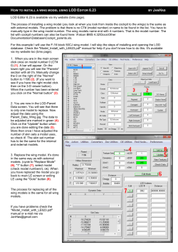


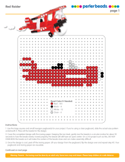
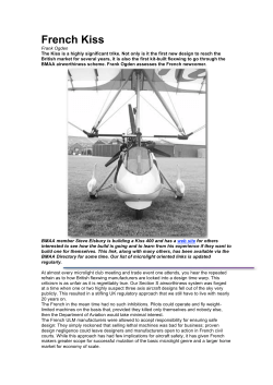


© Copyright 2026