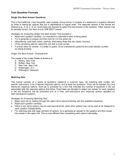
ST2238 Introductory Biostatistics
Lab 1
Lab 1:
Introduction to Minitab, paired &
two-sample t-tests
Q1: Effect of hypnosis in reducing pain
Hypnosis is sometimes used as a non-medicinal form of
pain relief. Price and Barbour1 recruited students to
a study in which they were exposed to painfully high
temperatures before and after hypnosis in order to assess whether hypnosis has any effect on their ability to
withstand pain. Participants indicated their (subjective) amount of pain on a 15cm strip. These pre- and
post-hypnosis measurements for eight participants are
reproduced below.
Subject
1
2
3
4
5
6
7
8
Before
6.6
6.5
9.0
10.3
11.3
8.1
6.3
11.6
After
6.8
2.4
7.4
8.5
8.1
6.1
3.4
2.0
(a) Why is a paired t-test more appropriate than a
two-sample t-test?
(b) Do the data look normally distributed?
(c) Perform a paired t-test to assess the hypothesis
that hypnosis has no effect. State your conclusions
carefully.
(d) What is a 95% confidence interval for the true
difference in mean subjective pain score before and after hypnosis?2
(e) What population does this sample represent?
(f) Why are the conclusions of this experiment dubious?
Q2: Ability of insects to detect floral iridescence
Iridescence is the change in colour of a surface when
viewed from different angles. Whitney et al.3 performed a laboratory experiment to assess whether floral iridescence is used to attract pollinating animals,
by making artificial flowers out of CDs that were either
iridescent or not, placing sweet substances on the iridescent tulip-castings and bitter on the non-iridescent
ones, and recording how frequently laboratory bees
identified the iridescent cast.
Whitney et al. report that as the ten bees gained
experience, they were more likely to visit the iridescent
casting. Specifically, they state that of the first 10
visits per bee, the mean and standard deviation of the
number of visits to the iridescent casting were 4.7 and
1.6, resp.; these were 8.1 and 1.3 on the last 10 (of 80)
visits.
Assume the number of visits in each of these groups
of ten are approximately normally distributed.
1
Price and Barbour, 1987, J. Abnormal Psychol. 96:46–51.
This is actually a stupid question included just for practice.
3
Whitney, Kolle, Andrew, Chittka, Steiner and Glover,
2009, Science 323:130–3.
2
Created by Alex Cook, National University of Singapore
(a) Assess the hypothesis that the standard deviations are the same in the “population” of na¨ıve and
experienced bees.
(b) Perform a two-sample t-test of the hypothesis
that bees do not learn with experience to identify iridescence. (Note, the authors took pains to ensure it
was colour alone that was guiding the bees.)
(c) Can you think of a better test for analysing the
results of the experiment than a two-sample t-test?
Q3: Do food resources decrease with distance from
barrier reefs?
Shima4 was interested in the habitat of the six bar
wrasse (Thalassoma hardwicke Bennett 1830), a marine reef fish that inhabits parts of French Polynesia.
He measured the settler density, defined as the number of juvenile fish per “unit” of settlement habitat, at
a series of sites at two distances (250m, 800m) from
the reef crests, in order to assess whether the resources
upon which the wrasse depends decrease with distance
from the reef crest.
The data can be downloaded from
http://courses.nus.edu.sg/course/stacar/internet/
st2238/data/thardwicke.txt
(a) Do the data look normal?
(b) Are the variances sufficiently similar that a twosample t-test can be performed?
(c) If so, perform a two-sample t-test of the hypothesis that the mean settler density is the same at the two
distances.
(d) Again, if the variances are similar enough, construct a confidence interval for the true difference between mean settler densities.
Hints:
Minitab is fairly intuitive, especially if you’ve ever used
a spreadsheet in the past. Functions can be called by
going to the menu along the top. It is also possible
to use a command line to call functions. This is very
useful when you are doing some repetitive analyses, as
you can copy and paste commands in without having
to go through each menu. To activate the command
line, go to Editor → Enable commands. Note that
this also allows you to see the commands equivalent
to the functions you call using the menus.
Minitab has a few sub-windows. One is the Worksheet. Your data go here, with one datum per cell.
Ensure the first element of the data is in row 1 (unlike excel, Minitab is fussy about this). Columns can
be referred to by their column number (e.g. C1) or
by a name if you assign one (this goes between the
“C1” row and row 1). Another sub-window is the Session window. This will contain the output of some
functions you run. It will also be where the command
prompt will appear if you use commands. There is also
a Project Manager Window (which I don’t know how
to use) and graphs will appear in their own windows.
A picture of these windows can be seen overleaf.
• To
start
Minitab,
Windows icon → All
programs → Minitab solutions → Minitab
4
Shima (2001), Ecology 82:2190–9.
Page 1
ST2238 Introductory Biostatistics
15 Statistical Software English
• To import data from a text file, File → Other
files → Import Special Test.
Choose the
columns to store the data in (this requires knowing
how many columns are in the data), click ok and
then browse for the file. If the data have headings,
Format allows lines to be skipped (i.e. you can skip
the top line containing the heading).
• To evaluate normality graphically, you can do a
histogram or what Minitab calls a probability plot.
• To do a histogram, Graph → Histogram, click
simple, and in the next pop-up, enter the columns
to plot histograms of in Graph variables. You
might like to display multiple histograms on the
same graph in different panels with the same scale
(on the x-axis) to get a feel for how the distributions vary. This can be effected by playing with
the options when you specify the columns for the
plot.
Lab 1
• You can create summary statistics of your data using Stat → Display Descriptive Statistics.
Ask me if any of the meaning of any of these isn’t
clear. Often students feel very attached to these
and lovingly reproduce them in reports. I advise
you are very selective in reporting summary statistics.
• You can save either the whole project or just an
individual worksheet. To save the project, File
→ Save Project. You might like to save each
week’s work as a separate project, perhaps with a
new worksheet per question.
• A very useful tool in Minitab is its calculator.
To access this Calc → calculator. This allows
you to manipulate the entries of one or more
columns and store them in another column or constant. [Constants are called “K1”, etc., and may
be viewed using the command line via print k1.]
This is a bit like excel’s functions, except you don’t
have to mess about with dragging and clicking.
• To do a probability plot, Graph → Probability
Plots, then choose single. The plot it makes
will have a straight line superimposed upon it.
The points should lie close to the line if the data
are normally distributed. Minitab has also superimposed some 95% confidence intervals (really,
it’s a [pointwise] confidence region): 95% of the
points should fall within this region. If too many
fall outwith the region, this is suggestive of nonnormality.
• Graphs can be saved to be imported into reports.
To do this, File → Save graph as. There is a
Mintab format, which no other program is likely to
be able to open. Save it in this format if you wish
to edit it in the future inside Minitab. Otherwise,
save as a jpeg or png. Unfortunately, Minitab like
much other windows software does not give the
option of saving as lossless vector graphics, such
as postscript or pdf.
• Graphs can be edited by double clicking on various parts of them. Personally, I hate the cream
background Minitab creates and the bold fonts for
axes labels. (If you want really good graphs, I recommend mastering R—but this involves a considerable investment in time.)
• A paired t-test can be done via Stat → Basic
Statistics → Paired t.
• A two-sample t-test can be done via Stat →
Basic Statistics → 2-sample t. Note: if you
have raw data in two columns, use the use
samples in different columns option. There is
also an option to perform the test based on summary statistics, i.e. the means, standard deviations and sample sizes. Note: I recommend ticking
the assume equal variances box. If you do not,
Minitab will do the version of the test that does
not assume equal variances, and the interpretation
will not be clear cut.
• An f-test of the equality of variances can be done
via Stat → Basic Statistics → 2 Variances
Created by Alex Cook, National University of Singapore
Page 2
ST2238 Introductory Biostatistics
Lab 2:
Non-parametrics,
gression
ANOVA, re-
Lab 2
st2238/data/burnout.txt
(a) Do the standard deviations look similar enough
to do an ANOVA?
(b) Perform an ANOVA. Is there any evidence of a
difference in burnout levels among the four groups of
physicians?
Q4: Sign and signed-rank tests
Q7: Two-way ANOVA
Catnip is commonly believed to be a drug that influences the behaviour of cats. A volunteer5 at an animal
shelter performed a study on the effect of the plant on
15 cats, by measuring the number of negative interactions each cat made during two 15 minute windows:
before and after administering the drug.
The data can be downloaded from
http://courses.nus.edu.sg/course/stacar/internet/
st2238/data/catnip.txt
(a) Do the data look normal?
(b) Use the sign test to test the hypothesis that
catnip has no effect on the behaviour of the cats.
(c) Try also the Wilcoxon signed-rank test to test
this hypothesis. Are your results consistent?
(d) You may also wish to perform a paired t-test.
What does the pattern of p-values tell you about the
tests?
(A question for all the ex-NSmen!) Levels of testosterone decrease during times of stress. This is particularly the case for soldiers. Morgan and colleagues8
measured testosterone in 12 soldiers during a military
exercise in which the (American) soldiers were “captured” and “interrogated”.
The data can be downloaded from
http://courses.nus.edu.sg/course/stacar/internet/
st2238/data/soldiers.txt
(a) Look at the data. Which appears most prominent: variability in adrenaline between soldiers or variability between times?
(b) Fit a two-way ANOVA using soldiers as blocks.
Does adrenaline change over the course of the exercise?
Does adrenaline differ between soldiers?
(c) Perform the following inappropriate analysis: a
one-way ANOVA without blocking on soldiers. How do
your conclusions change about the changing adrenaline
levels over the course of the experiment?
Q5: Rank-sum test
A liana is a kind of woody vine that grows in the
tropics. Ecologists6 measured abundance of liana (in
stems/ha) at randomly chosen plots in the Amazon.
Plots were randomised such that 34 were near the edge
of the forest (within 100m) and 34 were far from the
edge. The question that arises is: is the density of
lianas the same near the edge of the forest?
The data can be downloaded from
http://courses.nus.edu.sg/course/stacar/internet/
st2238/data/liana.txt
(a) Do the data look normal?
(b) Perform a Wilcoxon rank-sum test of the hypothesis that liana density near the forest edge is the
same as the density far from the forest edge.
(c) You may also wish to try a two-sample t-test
of the same hypothesis. Given your answer to the first
part of this question, which test would you prefer?
Q6: One-way ANOVA
L´
opez-Castillo and colleagues7 were interested in the
effect of stressful types of medicine on the burnout levels of physicians. They selected 25 medics from infectious disease (working mostly with AIDS patients), hæmophilia (also working with many AIDS patients), oncology and internal medicine wards in Spain, and measured their “burnout” level using the Maslach Burnout
Inventory questionnaire.
A summary of the data can be downloaded from
http://courses.nus.edu.sg/course/stacar/internet/
5
Jovan (2000). Stats 27:25–7
Laurance et al. (2001). Ecology 82:32–9
7
L´
opez-Castillo et al. (1999). Psychother. Pshcyosom.
68:348–56
6
Created by Alex Cook, National University of Singapore
Q8: Linear regression
Elephants are one of the most important mammals,
in part because they are the mammals least related
to man9 . They are therefore relatively well studied.
Being able to predict the gestation period of pregnant
elephant cows is important in preserving their numbers. A team of zoologists10 investigated the relationship between the cranial-rump length and gestational
age. Although they fitted a more complex model, we
shall assume a linear relationship is appropriate.
The data can be downloaded from
http://courses.nus.edu.sg/course/stacar/internet/
st2238/data/elephant.txt
(a) Plot the data. Does it appear there is a linear relationship between cranial-rump length and gestational
age?
(b) Perform a linear regression. What are your best
estimates of the slope and intercept?
(c) If an elephant cow presented to you with an
embryo of cranial-rump length 140cm, what would be
your best estimate of the age of her embryo?
Hints:
• The sign, Wilcoxon signed-rank and Wilcoxon
rank-sum tests can be found under Stat → Nonparametrics.
8
Morgan et al. (2000). Biol Pschyiatry 47:1889–901
Dawkins (2004) The Ancestor’s Tale—I strongly recommend this book!
10
Hildebrandt et al. (2007). Proc R Soc Lond B 274:323–31
9
Page 1
ST2238 Introductory Biostatistics
Lab 2
• Minitab calls the Wilcoxon signed-rank test the “1
sample Wilcoxon”.
• Minitab calls the Wilcoxon rank-sum test the
“Mann–Whitney”.
• ANOVA can be found under Stat → ANOVA.
• If you wish to do comparisons between pairs, there
is a Comparisons option in the ANOVA window. I
think “Fisher’s” corresponds most closely to what
we spoke about during class.
• Regression can be found under Stat → Regression
→ Regression.
• You may be interested in exploring the power
calculations Minitab allows. These allow you to
determine the minimum sample size needed to
achieve a specified power for particular parameter values. Check it out!
Created by Alex Cook, National University of Singapore
Page 2
ST2238 Introductory Biostatistics
Lab 3:
Multiple regression, binomial
test, Fisher’s exact test, and contingency tables
Q9: Multiple regression
Public health decision makers are often interested
in spatial heterogeneities in disease patterns, as these
patterns may indicate ways to improve care. A groundbreaking study was carried out on factors influencing
the propensity to lunacy in Massachusetts in the mid19th century, led by Edward Jarvis (who was not entirely co-incidently president of the American Statistical Association)11 . Recorded are multivariate data
from 14 counties, each of which has:
• Number of lunatics
Lab 3
deviations above the mean of the controls. This happened for 2 controls and 20 cancer patients.
Use Fisher’s exact test to assess whether pleiotrophin
is higher in cancer patients.
Q12: Contingency tables
Phenotypic traits are often correlated in spatially
distinct subpopulations. The Badeners are an ethnic
group in south-west Germany, in a region that is close
to the border of the northern and southern European
areas. Ammon collected data on hair and eye colour
among Badeners14 in the late 19th century, when the
German population was less homogenised than now.
These are presented below:
Hair:
Brown Black
Fair Red
Eye:
Brown
438
288
115
16
Grey/Green
1387
746
946
53
Blue
807
189 1768
47
Is there an association between hair and eye colour
in this ethnic group? Does this give any biological
insight?
• Distance to nearest mental health centre
Hints:
• County population (thousands, actually from
1950)
• County population density per square mile
• Percent of lunatics cared for at home
The data can be downloaded from
http://courses.nus.edu.sg/course/stacar/internet/
st2238/data/lunatics.txt
Using a multivariate linear regression, determine
what the factors are that influence lunacy occurence.
Based on your conclusions, what would you advise to
a policy maker?
• For the lunatics question, you may wish to start
by normalising the number of lunatics by dividing
by the county size. You may also wish to consider transforming distance to the nearest centre,
perhaps by taking the reciprocal.
Q10: Binomial test
Phillips and Smith12 wished to investigate whether
it was possible for terminally ill patients to postpone
death until after some significant date. They studies a
group of ethnic Chinese women living in California who
died within 1w of the harvest moon viewing festival. If
they were unable to postpone their death until after the
festival, we would expect the same number of deaths
before and after the festival date.
Of 103 women in the study, 70 died after and 33
died before the festival. Does this provide evidence
that death can be postponed?
Q11: Fisher’s exact test
Souttou and colleagues13 were interested in whether
the growth factor pleiotrophin was raised in individuals with pancreatic cancer. They measured this in 69
individuals—41 with the cancer and 28 controls—and
noted whether the level was more than two standard
11
For a more recent discussion, see Hunter (1987), Geograph
Rev 77:139–56
12
Phillips & Smith, 1990, J Am Med Assoc 263:1947–51
13
Souttou et al, 1998, J Natl Cancer Inst 90:1468–73
Created by Alex Cook, National University of Singapore
14
Ammon, 1899, Zur Anthropologie der Badener, Jena: Fis-
cher
Page 1