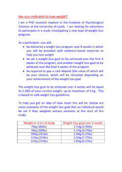
Bio 200 Lab 10 Two Sample Testing and ANOVA November 8 and 9, 2012 Tests for Independent Data with Unequal Variance Known Variance Unknown Variance Test Two-sample normal test with unequal variances Two-sample t-test with unequal variances Test Statistic 2 )−(µ1 −µ2 ) Z = (x√1 −x 2 2 1 −x2 )−(µ1 −µ2 ) t = (x√ 2 2 Distribution of Test Statistic Standard Normal tν Distribution σ1 /n1 +σ2 /n2 s1 /n1 +s2 /n2 Equation for degrees of freedom: ν= [(s21 /n1 ) + (s22 /n2 )]2 (s21 /n1 )2 /(n1 − 1) + (s22 /n2 )2 /(n2 − 1) Tests assuming unequal variances are more conservative and are therefore usually chosen unless you are certain that the variances are equal. Rule of Thumb: If the ratio of two sample standard deviations is between 0.5 and 2.0, use the equal variance t-test. Outside of 0.5 to 2.0, use the unequal variance t-test. 1 Question 1 Suppose you wish to determine if the mean body mass index (BMI) for male diabetics is equal to the mean for female diabetics. In each group, the distribution of indices is approximately normal. We cannot assume, however, that the variances are equal. A random sample of 207 male diabetics and 127 female diabetics was chosen and their bmi measured. The male diabetics had mean BMI x1 = 26.4 kg/m2 with standard deviation s1 = 3.3 kg/m2 . The female diabetics had mean BMI x2 = 25.4 kg/m2 with standard deviation s2 = 7 kg/m2 . Conduct a test at the α = .05 significance level to determine whether mean BMI is the same for males and females. (a) What type of test will you perform? Two sided, two sample t-test with unequal variances. We assume unequal variances because the problem statement says we cannot assume the variances are equal and by the rule of thumb since 7/3.3 > 2. (b) Perform the test by hand at a 0.05 level. H0 : µ1 = µ2 HA : µ1 6= µ2 α = .05. 2 )−(µ1 −µ2 ) = √(26.4−25.4)−(0) Z = (x√1 −x 2 2 2 2 σ1 /n1 +σ2 /n2 3.3 /207+7 /127 = 1.510244. P [|Z| > 1.510244] = 0.13. Fail to reject the null hypothesis: There is no evidence that the mean BMI is difference between males and females. (c) Perform the test in Stata using the ttesti command. Reference: Type: ttesti [n1] [mean1] [sd1] [n2] [mean2] [sd2], level([1-alpha]) ttesti 207 26.4 3.3 127 25.4 7 , level(95) unequal – What is the value of your test statistic? Two-sample t test with unequal variances ---------------------------------------------------------------------| Obs Mean Std. Err. Std. Dev. [95\% Conf. Interval] ---------+-----------------------------------------------------------x | 207 26.4 .2293659 3.3 25.94779 26.85221 y | 127 25.4 .6211496 7 24.17076 26.62924 ---------+-----------------------------------------------------------combined | 334 26.01 .2763842 5.05 25.47608 26.56344 ---------+-----------------------------------------------------------diff | 1 .6621446 -.3076163 2.307616 ---------------------------------------------------------------------diff = mean(x) - mean(y) t = 1.5102\\ Ho: diff = 0 Satterthwaite's degrees of freedom = 160.874\\ Ha: diff < 0 Ha: diff != 0 Ha: diff > 0\\ Pr(T < t) = 0.9335 Pr(|T| > |t|) = 0.1329 Pr(T > t) = 0.0665\\ 2 Statistic is distributed t with 160.874 degrees of freedom. (Approximately Z). Using tables: P (|t| > 1.51) = .0665 ∗ 2 = .13. Since p > .05, we do not reject the null hypothesis: there is no evidence that the mean BMI is different between males and females. – How could you have used the confidence interval for the population difference in means to test the null hypothesis? From the Stata output, use the diff row: (mean - t × s.e., mean + t × s.e.) = (1 - 1.96 × 0.662, 1 + 1.96 × 0.662) = (-0.307, 2.308). (Note: 1.96 is used here since the sample size is large enough that the Z can be used to approximate the t.) The 95% confidence interval for the differences covers the hypothesized difference (0), which is consistent with failing to reject the null. (Stata tip: To perform a hypothesis test on weight by sex, the Stata command is ttest weight==25, by(sex).) 3 ANOVA Analysis of variance, or ANOVA, is an extension of the two-sample equal variance t-test to k>2 groups. H0 : µ1 = µ2 = ... = µk HA : at least one pair of population means differ. The basic idea: compare two kinds of variation. 1. “Within-group variation” — variation of the individual values around the group mean s2W = (n1 − 1)s21 + (n2 − 1)s22 + ... + (nk − 1)s2k n1 + n2 + ... + nk − k 2. “Between-group variation” — variation of the group means around the overall mean s2B = (x1 − x)2 n1 + ... + xk − x)2 nk k−1 where x= n1 x1 + n1 x2 + ... + nk xk n1 + n2 + ... + nk Assumptions of ANOVA 1. Samples from the k populations are independent. 2. Samples from the k populations are normally distributed or sample size is large. 3. Standard deviations in the k populations are equal. i.e., σ1 = σ2 = ... = σk o Rule of Thumb- if the largest standard deviation is not more than twice the smallest, then okay to proceed with ANOVA. Test Statistic Fk−1;n−k = s2B s2W Two types of degrees of freedom: – numerator: k-1 (corresponds to the df for variation between groups) where k is the number of groups – denominator: n-k (corresponds to the df for variation within groups) where n is the total number of observations The F-statistic cannot assume negative values (do not double the p-value) 4 5 Question 2 We are interested in examining data from a study (discussed in the text) that investigates the effect of carbon monoxide exposure on patients with coronary artery disease, where baseline measurements of pulmonary function were examined across medical centers. Another characteristic that you might wish to investigate is age. The relevant measurements are saved on the course website in a data set called cad.dta. Values of age are saved under the variable name age and indicators of center are saved under center. (a) Use the “tab” command to summarize age for each center. What is the overall mean age? How many centers (groups)? What is the mean age and size of each group? . tab center, sum(age) medical | Summary of age (years) center | Mean Std. Dev. Freq. ------------+-----------------------------1.00 | 62.55 8.67 22 2.00 | 63.28 7.79 18 3.00 | 60.83 8.00 23 ------------+-----------------------------Total | 62.13 8.12 63 3 groups, x = 62.1, x1 = 62.55, x2 = 63.28, x3 = 60.83 n1 = 22, n2 = 18, n3 = 23 (b) Examine the histogram and boxplots of age for each center. Why is ANOVA an appropriate method for analyzing this data? Type: histogram age, by (center) Type: graph box age, over(center) From the boxplots and histograms, it seems reasonable to assume that the data are approximately normally distributed. Using the rule of thumb, we see that the greatest standard deviation, 8.67 is not more than twice the smallest standard deviation (7.79) so it is ok to assume our population standard deviations are equal. Finally, the centers represent 3 independent groups. 6 (c) Do ANOVA using Stata. Reference: oneway [variable of interest] [group variable] Type: oneway age center Analysis of Variance Source SS df MS F Prob > F -----------------------------------------------------------------------Between groups 66.6141226 2 33.3070613 0.50 0.6108 Within groups 4020.37 60 67.0061667 -----------------------------------------------------------------------Total 4086.98413 62 65.9190988 Bartlett's test for equal variances: chi2(2) = 0.2430 Prob>chi2 = 0.886 (d) What are the null and alternative hypotheses? What is alpha? H0 : µ1 = µ2 = µ3 HA : at least one pair of population means differ. α = .05. (e) What is the estimate of the within-group variance? (22−1)8.672 +(18−1)7.792 +(23−1)8.002 (22+18+23−3) = 4020/60 = 67.0 (f) What is the estimate of the between-groups variance? (62.55−62.13)2 22+(63.13−62.13)2 18+(60.83−62.13)2 23 3−1 = 66.6/2 = 33.3 (g) What is the value of the test statistic? 33.3/67.0 = .5 (h) What distribution does the test statistic follow? Fk−1,n−k = F3−1,63−3 = F2,60 (i) What is the p-value for the test? p = .61 from Stata (table in book shows p > .1) (j) Draw a conclusion for the test. Since p > 0.05, we fail to reject the null hypothesis: there is no evidence that there is a difference in age across the three centers. 7