
Manual for Wetland Ecosystem Services Protocol for Southeast Alaska (WESPAK‐SE)
Manual for Wetland Ecosystem Services Protocol for Southeast Alaska (WESPAK‐SE) by Paul R. Adamus, Ph.D1 Adamus Resource Assessment, Inc. for: Southeast Alaska Land Trust and US Fish & Wildlife Service Juneau, AK February 2012 – December 2013 and Oregon State University graduate faculty in Water Resources Graduate Program and Marine Resources Management Program. [email protected]. This manual was funded in part with qualified outer continental shelf oil and gas revenues by the Coastal Impact Assistance Program, U.S. Fish & Wildlife Service. 1 1 Table of Contents 1.0 Introduction ............................................................................................................................... 2 1.1 General Description .............................................................................................................. 2 1.2 Conceptual Basis ................................................................................................................... 3 1.3 Background ........................................................................................................................... 4 1.4 Limitations ............................................................................................................................ 7 1.5 Acknowledgments............................................................................................................... 10 2.0 Procedures for Using WESPAK-SE ...................................................................................... 11 2.1 Office Procedures................................................................................................................ 11 2.1.1 Obtain Aerial Images .................................................................................................. 11 2.1.2 Draw the Assessment Area (AA) Boundaries ............................................................ 12 2.1.3 Determine the Geographic Coordinates ...................................................................... 16 2.1.4 Interpret Aerial Images ............................................................................................... 17 2.1.5 Draw the Wetland’s Contributing Area (CA) ............................................................. 19 2.1.6 Obtain Required Information from Appendices and the WESPAK-SE Web Site ..... 21 2.1.7 Search for Other Useful Information .......................................................................... 21 2.2 Instructions for Field Component ...................................................................................... 22 2.2.1 Items to Take to the Field ........................................................................................... 22 2.2.2 Conduct the Field Assessment .................................................................................... 22 2.2.3 Shortcuts for Assessing Multiple Wetlands Rapidly .................................................. 24 2.3 Instructions for Entering, Interpreting, and Reporting the Data ........................................ 25 2.3.1 Enter the Data ............................................................................................................. 25 2.3.2 Evaluate Results .......................................................................................................... 25 2.3.3 Interpret the Results .................................................................................................... 26 2.3.4 Document the Assessment .......................................................................................... 29 3.0 Literature Cited ....................................................................................................................... 30 Appendix A. Maps Required to Answer Selected Form OF Questions ...................................... 31 Appendix B. Tabular Information Required to Answer Selected WESPAK-SE Questions ....... 35 Appendix C. Illustrations for Assessing Wetland Functions Using WESPAK-SE ..................... 44 Appendix D. Non-tidal Wetland: Data Forms F and S ................................................................. 48 Appendix E. Tidal Wetland: Data Forms T and S ........................................................................ 75 Appendix F. Descriptions of the WESPAK-SE models……………………(separate document) 2 1.0 Introduction 1.1 General Description Nature is complex, and varies enormously from place to place. As natural systems, wetlands are no exception. Thus, the use of one word or phrase describing a wetland’s type, or a short list of its characteristics, cannot meaningfully predict what a particular wetland does or the benefits it provides to human and biological communities. The roles of dozens of factors and their interactions must be considered and addressed systematically. Otherwise, assessments of what wetlands do‐‐ and therefore policies based on those assessments‐‐ will be on shaky scientific ground. Fortunately, there is a growing capacity to illustrate and encode some of natureʹs complexity in computer models. This, along with the commonplace availability of powerful personal computers that make those models quick and easy to use, has made some types of models simple to apply in the support of decisions and policies, while at the same time reassuring users and decision‐makers that assumptions in these models are transparent. The Wetland Ecosystem Services Protocol for Alaska: Southeast (WESPAK‐SE) is one such attempt. It is a standardized method and decision support tool for rapidly assessing ecosystem services (functions and values) of tidal and non‐ tidal wetlands of Southeast Alaska. Input data are categorical choices that are based on observations (not measurements) made during a single half‐day visit to a wetland, as well as from interpretation of generally available maps and existing resource information. The data are entered into an Excel spreadsheet that instantly generates scores for 18 functions and 20 values of a non‐tidal wetland, or 11 functions and values of a tidal wetland. Tidal wetlands are considered to include all wetlands inundated by tidal surface water at least once annually, e.g., during “king tides” regardless of their salinity. WESPAK‐SE is applicable to wetlands at all elevations of Southeast Alaska, from Yakutat south to the Canadian border. This Manual is not an operable version of WESPAK‐SE. That is contained in accompanying Excel spreadsheets, one for non‐tidal and one for tidal wetlands. WESPAK‐SE is intended to fill a need for rapid, standardized, field‐based assessment of wetland ecosystem services such as provided because few agencies or organizations have sufficient personnel who can interpret the implications of wetland hydrology, soils, and biogeochemical interactions during a brief site visit, as well as having the skills to identify all of the region’s wetland plants and animals. Moreover, biodiversity 3 alone cannot validly be used to predict many of a wetland’s ecosystem services that are valued by society. WESPAK‐SE uses assessments of weighted ecological characteristics (indicators) to generate scores for a wetland’s functions and values. The number of indicators that is applied to estimate a particular wetland function or value depends on what the function or value is. The indicators are combined using mathematical formulas (models) to generate the score for each wetland function or value. The models are logic‐ based rather than deterministic. Together they provide a profile of “what a wetland does.” WESPAK‐SE indicators and models attempt to incorporate the best and most recent scientific knowledge available on the ecosystem services of wetlands. Each indicator has a suite of conditions, e.g., different categories of percent‐slope. For each wetland function or value, ranks have been pre‐assigned to all conditions potentially associated with each indicator used to predict the level of that function or value. The ranks can be viewed in column E of the individual worksheets. For most models of wetland functions, the indicators were grouped by the underlying processes they inform. Weights were then assigned both to individual indicators within a process, and the processes that comprise a function. Indicator and process selection was based on the author’s experience and review of much of the literature he compiled initially in an indexed bibliography of science relevant to Southeast Alaskan ecosystem services (available electronically from SEAL Trust or the author). 1.2 Conceptual Basis WESPAK‐SE provides models for both functions and values. It is very important to understand the conceptual difference. Functions are what a wetland potentially does, such as store water. Values attempt to answer the “So What?” question, partly by considering where a wetland is positioned relative to people or features that might benefit from its services, and whether its species or habitats have special designations. For example, when wetlands retain or remove nutrients, this can be valuable for protecting the quality of downstream waters in some settings (e.g., urban runoff impacts to estuaries) but undesirable in others (e.g., salmon rearing streams, where nutrients are needed to support algae and invertebrate components of the salmonid food chain). The Value score that WESPAK‐SE computes accounts for these differences, separately from the Function score. In concept, wetland ecosystem services are the combination of functions and the values of those functions, judged individually. Thus, 4 for a wetland to be considered as providing a high level of services, both its functions and the values (or recognized potential value) of those functions should be high. Fundamentally, the levels and types of functions that wetlands individually and collectively provide are determined by the processes and disturbances that affect the movement and other characteristics of water, soil/sediment, plants, and animals (Zedler & Kercher 2005, Euliss et al. 2008). In particular, the frequency, duration, magnitude and timing of these processes and disturbances shapes a given wetland’s functions (Smith et al. 2008). Climate, geology, topographic position, and land use strongly influence all of these. Several analyses (e.g., Hansson et al. 2005, Adamus et al. 2009) have concluded that it is unlikely to have all functions occurring at a high level in a single wetland, even in the most pristine wetlands. 1.3 Background WESPAK‐SE is a regionalized modification of ORWAP 1 , the Oregon Rapid Wetland Assessment Protocol, developed by the same author from 2006 to 2009, which built on indicator‐function relationships first described by the author in the early 1980s and in several agency publications and methods since then, including the 1993 Juneau Wetlands Management Plan. The State of Oregon, in collaboration with the US Army Corps of Engineers Portland District, has required ORWAP assessments since 2009 for all major wetlands permitting and mitigation. The province of Alberta has also regionalized a generic version of the Oregon method for their needs, and Nova Scotia intends to begin such an effort in 2014. If interest is sufficient, WESPAK‐SE could be modified for use elsewhere in Alaska. In 2009, at the behest of an Interagency Review Team (IRT) and Southeast Alaska Land Trust (SEAL Trust), an independent consulting firm was contracted to review and critique 16 wetland rapid assessment methods potentially applicable to Southeast Alaska. They selected ORWAP/WESPAK‐SE and recommended its adaptation and calibration in the region (CH2M Hill, 2010). The City and Borough of Juneau is considering using this WESPAK‐SE method to re‐prioritize its wetlands in 2014, and SEAL Trust intends to use it in collaboration with the US Army Corps of Engineers for their In‐Lieu Fee Mitigation program. As of October 2013, three training sessions for agency staff and consultants have been held, and more are anticipated. 1 Hhttp://oregonstatelands.us/DSL/WETLAND/or_wet_prot.shtml 5 WESPAK‐SE is intended to help address a policy goal of “no net loss” of wetlands, as that goal pertains not only to wetland acreage but also to the ecosystem services (functions and values) that wetlands provide naturally. By providing these services, well‐functioning wetlands can reduce the need for humans to construct alternative infrastructure necessary to provide those services, often at much higher cost (Costanza et al. 1997, Finlayson et al. 2005, Euliss et al. 2008). In addition, many laws and policies require compensation for wetland impacts, and further require that wetland functions and values be the basis for considering the adequacy of compensation. A few other methods developed for rapidly assessing wetlands in this region are briefly summarized in Appendix A. Field‐testing is an essential part of developing methods such as WESPAK‐SE, both for improving the data forms and models, and for determining the range of scores that can be expected, i.e., the calibration process. Using draft versions of the data forms, the author assessed 32 wetlands throughout Southeast Alaska during September 2011 (Table 1). The wetlands were in four subregions: Juneau, Haines, Sitka, and Ketchikan. In each subregion, attempts were made to visit at least one fen, marsh, hillslope bog, hillslope forest, and riverine or tidal wetland. The assessed wetlands are not a random or systematically balanced sample of all wetlands currently mapped in Southeast Alaska. That is because access to most parts of the region is challenging and funding did not permit such a structured selection process. During 2013, additional sites from other parts of the region were selected using a statistical procedure. They were then visited and assessed, with support from SEAL Trust and the US Fish and Wildlife Service, to provide a broader and more balanced basis for comparison of function and value scores. Separately, 24 additional wetlands in the Juneau area were visited and assessed in 2013 with support from the City and Borough of Juneau. Repeatability (reproducibility) of results was quantified with the help of 5 volunteers who independently assessed the same 5 non‐tidal and 3 tidal wetlands. As wetlands were assessed during the calibration work in 2011 and 2013, data forms were edited slightly to improve clarity. In some cases new indicators that seemed useful were added, and others dropped. After all visits had been completed, final versions of the data forms were prepared, formulas were drafted for computing scores (i.e., models), and scores were computed. Model formulas were occasionally adjusted at this stage to reflect the author’s perceptions of relative levels of functions at the sites. Final versions of the models were then applied to the data and the summary statistics shown in the Scores worksheet were calculated. 6 Table 1. Geographic coordinates for WESPAK‐SE version 1.0 calibration sites assessed in 2011 Latitude NON‐TIDAL SITES Haines Homestead Haines Chilkat Fen Haines Chilkat Isolated Pond Haines Riparian Restored Juneau Switzer Cr. Juneau Vanderbilt Cr. Juneau Duck Cr Nazarene Juneau NS9 Fred Meyer Juneau NS6 Montana Swamp Juneau NS2 Eaglecrest Bog Juneau NS2 FishCr WeatherStn Juneau NS3 ADOT shrub bog Juneau Eaglecrest Dʹ Amore Bog GC bog GC fen GC forested Althea GC forestedTrib GC marsh GC shrub Bog Sitka Gavin Hill Bog Sitka Gravel Pit Forested Sitka Indian R. floodplain Sitka Indian R. shrub bog Ketchikan Gravina Bog Pond Ketchikan Gravina South Bog Ketchikan montane Shrub Bog Ketchikan Point Higgins Ketchikan Ward Lake Ketchikan Ward River TIDAL SITES: Sitka Starrigavan Juneau Mendenhall Haines tidal forest Haines tidal flat Longitude 59.16260 59.28330 59.34498 59.24190 58.36590 58.35580 58.37600 58.36177 58.39323 58.31400 58.33570 58.32423 58.29610 58.11164 58.11290 58.11321 58.11364 58.12048 58.11046 57.05749 57.10823 57.06046 57.06074 55.32752 55.31408 55.42682 55.46081 55.40894 55.44297 ‐135.35930 ‐135.68040 ‐135.76940 ‐135.44560 ‐134.49610 ‐134.48770 ‐134.57750 ‐134.56990 ‐134.59387 ‐134.55600 ‐134.56400 ‐134.50053 ‐134.55030 ‐134.74887 ‐134.74570 ‐134.75323 ‐134.74570 ‐134.74703 ‐134.74329 ‐135.32935 ‐135.38595 ‐135.30593 ‐135.30918 ‐131.68344 ‐131.65961 ‐131.60895 ‐131.82872 ‐131.69873 ‐131.62492 57.13190 58.35304 59.23539 59.21710 ‐135.36657 ‐134.51614 ‐135.47631 ‐135.45110 7 Table 1. Geographic coordinates for WESPAK‐SE version 1.2 Juneau calibration sites assessed in 2013 Site Name Cowie Bog Cowie Marsh Cowie Uplift Meadow Lower Mendenhall Mendenhall Trail Pond Mendenhall Riparian Mendenhall School Rotary Park Switzer Meadow Mendenhall Peninsula north Egan ditch Snipe Switzer DOT ditch Lakeshore Glacier Duck N Glacier Duck S DEC north DEC south B&B Hanger LaRouse Yandukin Peterson fen Peterson bog Peterson riparian Mendenhall Peninsula south Fish Cr. Tidal Pond Latitude 58.6481 58.6549 58.6738 58.372 58.3773 58.3779 58.378 58.3813 58.3608 58.3523 58.3588 58.3594 58.3592 58.3816 58.3723 58.3714 58.3677 58.3666 58.3625 58.3714 58.3625 58.3603 58.2996 58.2989 58.2877 58.3484 58.3301 Longitude ‐134.9346 ‐134.9393 ‐134.9635 ‐134.6045 ‐134.6004 ‐134.5971 ‐134.5954 ‐134.586 ‐134.5075 ‐134.6357 ‐134.5429 ‐134.5541 ‐134.5258 ‐134.5751 ‐134.5849 ‐134.5855 ‐134.5895 ‐134.5901 ‐134.5875 ‐134.5855 ‐134.5913 ‐134.5798 ‐134.6724 ‐134.6751 ‐134.6695 ‐134.6383 ‐134.5997 1.4 Limitations WESPAK‐SE is not intended to answer all questions about wetlands. Users should understand the following important limitations: 1. WESPAK‐SE does not change any current procedures for determining wetland jurisdictional status, delineating wetland boundaries, or requirements for monitoring wetland projects. 8 2. The intended users are wetland specialists for government agencies, natural resource organizations, and consulting companies, who are skilled in conducting jurisdictional delineations of wetlands. Users should be able to (a) recognize most common wetland plants, (b) determine soil texture, (c) understand wetland hydrology, (d) delineate wetland contributing area (catchment) boundaries from a topographic map, (e) access and acquire information from the internet, and (f) enter data in Microsoft Excel® (1997 or later version). For field application of WESPAK‐SE, a multidisciplinary team is encouraged but not required. Training in the use of WESPAK‐SE also is encouraged but not required. 3. The numeric estimates WESPAK‐SE provides of wetland functions, values, and other attributes are not actual measures of those attributes, nor are the data combined using mechanistic models of ecosystem processes. Rather, WESPAK‐SE scores are estimates of those attributes arrived at by using standardized criteria (models). The models systematically combine well‐accepted indicators in a logically sophisticated manner that attempts to recognize context‐specific, functionally contingent relationships among indicators. As is true of all other rapid assessment methods, WESPAK‐SE’s scoring models have not been validated in the sense of comparing their outputs with those from long‐term direct measurement of wetland processes. That is the case because the time and cost of making the measurements necessary to fully determine model accuracy would be exorbitant. Nonetheless, the lack of validation is not, by itself, sufficient reason to avoid use of any standardized rapid method, because the only practical alternative—relying entirely on non‐systematic judgments (best professional judgment)—is not demonstrably better in many cases. When properly applied, WESPAK‐SE’s scoring models and their indicators are believed to adequately describe the relative effectiveness of a wetland for performing particular functions. 4. WESPAK‐SE may be used to augment the interpretations of a subject professional (e.g., a fisheries biologist, plant ecologist, ornithologist, hydrologist, biogeochemist) when such expertise is available. WESPAK‐SE outputs, like those of other rapid methods, are not necessarily more accurate than judgments of a subject expert, partly because WESPAK‐SE’s spreadsheet models lack the intuitiveness and integrative skills of an actual person knowledgeable of a particular function. Also, a model cannot anticipate every situation that may occur in nature. WESPAK‐SE outputs should always be screened by the user to see if they “make sense.” Nonetheless, WESPAK‐SE’s scoring models provide a degree of standardization, balance, and comprehensiveness that seldom is obtainable from a single expert. 9 5. WESPAK‐SE’s logic‐based process for combining indicators has attempted to reflect currently‐understood paradigms of wetland hydrology, biogeochemistry, and ecology. Still, the scientific understanding of wetlands is far less than optimal to support, as confidently as some might desire, the models WESPAK‐SE and other rapid methods use to score wetland attributes. To provide transparency about this uncertainty, in the Rationales column of the WESPAK‐SE worksheets for individual functions, some of the more significant alternative or confounding interpretations are noted for indicators used in that function’s scoring model. 6. WESPAK‐SE does not assess all functions, values, and services that a wetland might support. In particular, WESPAK‐SE does not assess the suitability of a wetland as habitat for any individual wildlife or plant species. The 18 functions and 21 values WESPAK‐SE assesses are those most commonly ascribed to wetlands. 7. If two wetlands have similar effectiveness scores for a function and its value, the larger wetland is usually more likely to provide a greater total level of the associated ecosystem service. However, the relationship between wetland size and the total level of a service delivered is not necessarily linear. For example, if its characteristics make a particular wetland ineffective for storing or purifying water, or for supporting particular plants and animals, then simply increasing its size by adding more wetland having the same characteristics will usually not increase the total amount of water stored or purified, or plants and animals supported. The threshold below which a wetland’s characteristics make it completely ineffective is unknown in many cases. Where scientific evidence has suggested that wetland size may benefit a function in a greater‐than‐linear manner, WESPAK‐SE has included wetland size as an indicator for that function. Those functions are Waterbird Feeding, Waterbird Nesting, Songbirds‐ Mammals, and Pollinators. 8. In some wetlands, the scores that WESPAK‐SE’s models generate may not be sufficiently sensitive to detect, in the short term, mild changes in some functions. For example, WESPAK‐SE is not intended to measure small year‐to‐year changes in a slowly‐recovering restored wetland, or minor changes in specific functions, as potentially associated with limited “enhancement” activities such as weed control. Nonetheless, in such situations, WESPAK‐SE can use information about a project to predict the likely direction of the change for a wide array of functions. Quantifying the actual change will often require more intensive (not rapid) measurement protocols that are complementary. 10 9. WESPAK‐SE outputs are not intended to address the important question, “Is a proposed or previous wetland creation or enhancement project in a geomorphically appropriate location?” That is, is the wetland in a location where key processes can be expected to adaptively sustain the wetland and the particular functions which those of its type usually support, e.g., its “site potential?” Although WESPAK‐SE uses many landscape‐scale indicators to estimate functions and values of a wetland, WESPAK‐SE is less practical for identifying the relative influence of multiple processes that support a single wetland. 1.5 Acknowledgments I thank Diane Mayer of SEAL Trust and Hans Ehlert of CH2M Hill for initiating this effort with their recognition in 2010 of the importance of standardized practical tools for the field‐based assessment of ecosystem services of wetlands, and for their support of what became WESPAK‐SE. I am also grateful to the US Fish and Wildlife Service, and particularly to Steve Brockman and Neil Stichert of the Juneau Office, for recognizing the potential of this tool for their programs and responding with financial support and scientific information. I thank the City and Borough of Juneau (CBJ) for their support, long before that, of my 1986‐87 wetlands study which resulted in their initial wetlands management plan and laid a foundation for the current efforts. For initiating and administering the contract supporting this updated refinement of WESPAK‐SE, and her tireless efforts to ensure that wetland decisions are informed by the best available science, I particularly thank Teri Camery of the CBJ Community Development Department. Many experts provided invaluable information which helped strengthen the WESPAK‐SE models either during the structured peer review workshops or in separate correspondence during 2010 or 2013. I thank Bob Armstrong, Ellen Anderson, Koren Bosworth, Terry Brock, Richard Carstensen, Dave D’Amore, Chiska Derr, Jackie Foss, Lisa Hoferkamp, John Hudson, Dennis Landwehr, Steve Paustian, Andrew Piston, Deb Rudis, James Rypkema, James Ray, Mark Schwan, Neil Stichert, David Tallmon, Gus Van Vliet, Brenda Wright, Sadie Wright, and Johnny Zutz. Members of the CBJ Wetlands Review Board also made useful suggestions. A critical component of WESPAK‐SE – the Southeast Alaska wetlands internet portal – was the masterpiece of Kim Homan, with help from Jason Seifert. The important task of testing the WESPAK‐ SE’s repeatability was accomplished by Koren Bosworth, Matt Brody, Chiska Derr, Nena Horne, John Hudson, and Rod Lacey, with administrative help from Chrissy McNally of the CBJ Community Development Department. 11 2.0 Procedures for Using WESPAK-SE You will be completing three forms: an office form (OF); and two field forms (F and S). In a nutshell, the procedure is as follows: 1. Read this entire section (Section 2) before proceeding to complete the forms for the first time. 2. Download the most recent version of the WESPAK‐SE_ Calculator (Tidal and Non‐tidal versions) spreadsheet from the Southeast Alaska Land Trust web site: http://southeastalaskalandtrust.org/wetland‐mitigation‐sponsor/wespak‐se/ 3. Also download and print (from the same sites) the PDF versions of data forms F and S. Do not print form OF or anything from the Excel spreadsheet at this point. 4. Complete the “office” component, which involves viewing aerial imagery and filling out the form OF worksheet in the WESPAK‐SE Calculator file, mainly by obtaining map information from the University of Alaska’s WESPAK‐SE Wetlands Module web site described below. 5. Visit the wetland and complete the “field” component by filling out data forms F& S. Then refine your answers to questions on form OF if necessary. 6. Process and interpret the results. 2.1 Office Procedures Begin the office component of the assessment with the electronic version of form OF in the file WESPAK‐SE_Calculator_Nontidal.xls or WESPAK‐SE_Calculator_Tidal.xls. When you open that file, you may get a message asking if you want to enable “macros.” Mark yes; the macros in this file will not harm your computer. They are necessary to automate all the calculations. 2.1.1 Obtain Aerial Images You will need a recent aerial image of the wetland of interest in order to answer several of the questions in form OF. There are many sources of aerial imagery that can be viewed for free online. Either of these will be adequate: • Google Earth web site: http://earth.google.com/downloadearth.html Easy to access and use, but image clarity is poor for some parts of Southeast Alaska. • WESPAK‐SE Wetlands Module web site: http://seakgis.alaska.edu/flex/wetlands/ 12 2.1.2 Draw the Assessment Area (AA) Boundaries A key term is assessment area (AA). That area is usually the same as that of an entire wetland polygon, with its boundary obtained from an existing map, a field delineation, or your own interpretation of aerial images and topography. The AA preferably will consist of the entire wetland plus, in some cases, some or all of the adjoining unvegetated water (see below). However, in some cases you may draw the AA to encompass just part of a wetland, e.g., the part in which impacts or conservation actions are anticipated. Other instances might include instances where: • The wetland extends across property lines and access permission to part of the wetland was not granted. • The wetland is so large (e.g., >100 acres) and internally varied that an accurate assessment cannot be completed in a day. Boundaries of the AA should be based mainly on hydrologic connectivity. Depending on purposes of the assessment, they normally should not be based solely on property lines, fence lines, mapped soil series, vegetation associations, elevation zones, land use or land use designations. The AA boundaries may need to be adjusted during the field component, but for WESPAK‐SE’s purposes you don’t need to delineate the AA boundary with the high level of precision customary for legal delineations. Nonetheless, where you draw the boundaries of the AA can dramatically influence the resulting scores. If you delimit an AA that does not occupy all of a wetland, you should report the approximate percent of the wetland it occupies. A space is provided for this in the CoverPg worksheet of the WESPAK‐SE Calculator. Similarly, you should estimate and note the approximate percent of the mapped AA you were able to visit (taking into account both physical restrictions and private property restrictions). Here are guidelines for delineating the AA in some specific situations: a. Dissected Wetland. If a wetland that once was a contiguous unit is now divided or separated from its formerly contiguous part by a road or dike (Figure 1), assess the two units separately unless a functioning culvert, water control structure, or other opening connects them, and their water levels usually are simultaneously at about the same level. 13 f Figure 1. Dissected Wetland. A wetland is crossed by a road or filled area. Separate the wetland into two AA’s and assess separately if A and B have different water levels and circulation between them is significantly impeded. b. Fringe Wetland. If a wetland is a fringe wetland (that is, it borders a bay, estuary, pond, or river in which the contiguous stretch of open water is >3x wider than the wetland), the AA should include just the vegetated wetland, not the adjoining water (unless the method specifically directs you to answer a question about that). An exception is if the contiguous water body including the wetland is smaller than 20 acres, e.g., a pond. In that case, the water body itself (regardless of depth) should be included as well as the wetland (Figure 2). 14 Figure 2. Fringe Wetland Type 1. The average width of the open water area is more than 3x wider than the average width of the wetland, making this a fringe wetland. If the entire polygon is smaller than 20 acres, the AA should include the open water. If larger, the AA should include only the wetland. c. Fringe Wetland Patches. If patches of fringe wetlands share the same margin of a river, lake, or estuary and are separated from each other by upland over a distance of greater than 100 ft, they should be assessed as separate AA’s (Figure 3) unless they appear to be the same in nearly every aspect (dominant vegetation, soil texture, hydrology, landscape position, Cowardin classification, adjoining land use, etc.) and are within 1000 ft. of each other. 15 Figure 3. Fringe Wetland Type 2 (fringe wetland patches). Wetland patches B and C would be included in the same AA if separated by no more than 100 ft. by water, bare substrate, algal flats, or upland. Wetland patches A and D would be in the same AA if separated by 100 ft or less, or if they are within 1000 ft of each other and their vegetation, soil texture, water regime, and adjoining land use is the same. d. Lake Wetland With Tributary. If a lacustrine (lakeside) wetland is intersected by an inflowing stream, the wetland should be considered lacustrine except for the part that is more subject to seasonal overflow from the stream than from fluctuations in lake levels. That part should be assessed separately. e. Wetland Mosaic. If the wetland is a patch in a mosaic of wetlands within uplands or other non‐wetland waters (Figure 4) and none of the above rules apply, the entire mosaic should be considered and delimited as one AA if: • Each patch of wetland is smaller than 1 acre, and • Each patch is less than 50 ft from its nearest neighboring wetland and is not separated from them by impervious surface, and • The areas of vegetated wetland are more than 50% of the total area. The total area is the wetlands plus other areas that are between the wetlands (such as uplands, open water, and mudflats). 16 Figure 4. Wetland Mosaic Assessment Area (AA). In this diagram the dark line defines the mosaic. The circles are wetlands and the areas between them are upland. Wetlands C, D, E, F, and G comprise a mosaic because they occupy more than 50% of the total area bounded by the dark line. Wetland B is excluded because it is larger than 1 acre. Wetlands A and H are excluded because each is >100 ft from its closest neighbor. f. Tidal/Non‐Tidal Wetland. If any vegetated part of the AA is tidal (receives tide‐ driven surface water on any day during an average year), assess that part separately from the non‐tidal part, using the WESPAK‐SE data form for Tidal Wetlands. 2.1.3 Determine the Geographic Coordinates To expedite finding your AA in an aerial image, you may input its geographic coordinates (latitude and longitude). Determine the latitude and longitude of the AA’s approximate center in decimal‐degrees, e.g., 45.2434, ‐123.3425. For WESPAK‐SE’s purposes, the precision of the coordinates need not be any greater than about half of the width of the wetland. If the wetland’s coordinates have not already been determined in the field using a GPS (NAD83 datum), determine them as follows: Using Google Earth: a. After downloading Google Earth (if you don’t already have it) from the internet, go to the Tools dropdown menu and select Options. Select the 3D View tab, check decimal degrees, and hit Apply. 17 b. If you know the lat/long in degrees minutes seconds (rather than decimal degrees) you can type in that value and Google Earth will convert it and display in the bottom center of the window. c. Alternatively, if you enter a street address, cross streets, or other information into the “Fly To” space, the map will zoom to that approximate location. Locate your wetland and move the cursor to the center of the part you wish to assess. The correct Lat / Long is displayed in the bottom left center of the window. Using the WESPAK‐SE Wetlands Module: a. After accessing the web site, zoom to your AA and read the coordinates (latitude, longitude) in the lower left. b. Alternatively, in the toolbar at the top, click on the Find a Location (second) icon: ^ Then in the pop‐up menu, click on the pushpin icon and enter the lat/long, or click on the mailbox icon and enter an address. 2.1.4 Interpret Aerial Images You will use aerial images, zoomed at various scales, to answer WESPAK‐SE questions OF1 through OF16 (non‐tidal wetlands), as well as OF1‐OF11 and T26‐30 (tidal wetlands). Preferably, respond to these questions using the imagery before you visit the wetland. Record your responses directly in the spreadsheet (form OF worksheet tab at bottom of page), print the completed form, and take it with you during the site visit. Upon visiting the site, modify your estimates if appropriate based on your observations. First, zooming to its location, bring up an aerial of your AA. In the WESPAK‐SE Wetlands Module, click on the left end of the “Select Your Basemap” menu in the upper left and select “Best Available Data Layer” or “Bing Imagery.” Also, one WESPAK‐SE question requires you to view a topographic map. To do so, select instead “Topographic” in the “Select Your Basemap” menu. Note that several questions ask you to measure distances from your AA of specified features or in a few cases, the area of a feature. To do so, go online to this toolbar in the WESPAK‐SE Wetlands Module and click on the Measure icon: 18 ^ The following menu pops up: To measure distance, click on the jagged line symbol in the top left and then halfway down the menu where it says Distance Units click on Miles or Feet. Then go to the website’s main map or aerial, place your cursor on the AA, click it, drag it to the feature being measured, and double‐click. The distance measurement will appear on the map. If it’s hard to read, go back to the bottom of the pop‐up menu and change the Color. To measure area, click on the polygon symbol in the top right and then halfway down the menu where it says Area Units click on Acres. Then go to the website’s main map or aerial, place your cursor on one point along the edge of the AA, click it, move to another point on the edge, click it, and so forth until you’ve enclosed the entire polygon. Then double‐click and the area measurement (as well as the length of the polygon’s perimeter) will appear on the map. Also note that several questions ask you to estimate conditions within a landscape (buffer) of radius 0.5 mile or 2 miles centered on your AA. To create a circle of that radius, go online to this toolbar in the WESPAK‐SE Wetlands Module and click on the Buffer/Range icon: 19 The following menu pops up: ^ Click on the point (solid circle) in the upper left of the above menu, then place your cursor in the center of the AA, click, and return to the Buffer/Range menu. Under the heading “Buffer Properties” click the buffer radius desired (0.5 or 2 miles), then click the white box in the lower middle of the menu. A buffer of that size should appear on the map, surrounding the point you placed. Don’t be concerned that the buffer isn’t perfectly round – it is accounting for geographic and elevational distortion. If the buffer is too dense to adequately view features beneath it, decrease the Opacity in the above menu. When you’re done, click Clear and then the trash can symbol to the right of the buffer icon at the bottom of the above menu. To estimate the percentages of a given land cover within the buffer circle, imagine all the patches of that type being “squeezed together” and determine the approximate fraction of the circle they would occupy. Note that the questions for “natural land cover” and “herbaceous open land” ask the percentage of the land area of the circle that is occupied by the specified land cover, whereas the questions for “ponded water” use the entire circle, including large lakes but not ocean. 2.1.5 Draw the Wetland’s Contributing Area (CA) The CA is the drainage area, catchment area, or contributing upland that feeds the wetland (Figure 5). It includes the AA plus all areas uphill from the AA until a ridge or topographic rise is reached, often many miles away, beyond which water would travel 20 in a direction that would not take it to the AA. The water does not need to travel on the land surface; it may reach the AA slowly as shallow subsurface seepage 2 . The lowest point of a CA is the lowest point in the AA. The CA’s highest point will be along a ridgeline or topographic mound. Although it is possible that roads, tile drains, and other diversions that run perpendicular to the slope may interfere with movement of runoff or groundwater into a wetland (at least seasonally), it is virtually impossible to determine their relative influence without detailed maps and hydrologic modeling. Therefore, in most cases draw the CA as it would exist without existing infrastructure, i.e., based solely on natural topography as depicted in the topographic map. The only exception is where maps, aerial images, or field inspections show artificial ditches or drains that obviously intercept and divert a substantial part of the runoff before it reaches the wetland, or where a runoff‐blocking berm, dike, or elevated road adjoins all of a wetland’s uphill perimeter. CA W Figure 5. Delimiting a wetland’s Contributing Area (CA). Wetland (to the right of the “W”) is fed by its Contributing Area (CA) whose boundary is represented by the red line. The dark arrow denotes flow of water downgradient within the CA. The light arrows denote the likely path of water away from the CA and into adjoining drainages, as interpreted from the topography. Note that the CA boundary crosses a stream at only one point, that being the outlet of the wetland. 2 There are often situations where subsurface flow (especially deep groundwater), that potentially feeds a wetland, ignores such topographic divides. However, due to the limitations imposed by rapid assessment, no attempt should be made to account for that process. 21 The CA may include other wetlands and ponds, even those without outlets, if they’re at a higher elevation. Normally, the boundary of a CA will cross a stream at only one point— at the CA’s and AA’s outlet, if it has one. Do not include contiguous perennial deep waters at the same elevation (such as a lake, river, or bay) unless requested by the question. Especially in urban areas and areas of flat terrain, the CA boundaries can be somewhat subjective and estimation in the field may be preferable. However, for WESPAK‐SE’s purposes a high degree of precision is not needed. 2.1.6 Obtain Required Information from Appendices and the WESPAK‐SE Web Site To complete the office phase of WESPAK‐SE (form OF), you must obtain specific information primarily from a Wetlands Module web site created and hosted by the UAS’s Southeast Alaska GIS Library: http://seakgis.alaska.edu/flex/wetlands/ Instructions for finding the needed information on this web site are provided in the individual questions on WESPAK‐SE form OF. As you look for particular layers (maps) in the web site’s Table of Contents, note that you can expand the list shown by dragging the bottom right corner. Also, the web site also has a short tutorial that provides helpful guidance – click on the “?” icon in the toolbar on the top of the main page. For just a few questions, you also will need to extract information from maps and tables in Appendices A and B. Note that if information from the Module or appendices conflicts with your field observations, the field observations should usually control. 2.1.7 Search for Other Useful Information While completing a WESPAK‐SE assessment, you should ask the land owner, land manager, or neighbors about the annual extent and depth of high and low water, as well as the annual duration of surface‐water connection with streams and other wetlands. Even where flood marks are pronounced, such characteristics are difficult to estimate visually during a single wetland visit. Local offices of municipal, state, tribal, and federal agencies should also be contacted for information that will improve the accuracy of your assessment. An online search of the name of a nearby feature can sometimes be productive. Also, for some areas, you can go online and easily view aerial images from other seasons and/or years. To do so, open GoogleEarth, zoom to your location, and click on the sundial icon in the toolbar in the middle top of the page. Finally, note that soils information from wider parts of the region will eventually 22 become available online at http://websoilsurvey.nrcs.usda.gov/app/HomePage.htm . This can be used as an aid in identifying wetlands and wetland contributing areas with high risk of landslides or soil erosion. 2.2 Instructions for Field Component The field component involves visiting as much of the AA as possible, filling out the two field forms (F and S), and verifying, as needed, answers previously given on form OF. This component will generally require fewer than three hours (large or complex sites may take longer). If circumstances allow, visit the AA during both the wettest and driest times of year (if tidal, also during high and low tide). If you cannot, you must rely more on the aerial imagery, maps, other office information, field indicators, and discussions with the landowner and other knowledgeable sources. 2.2.1 Items to Take to the Field Take the following with you into the field: ___Blank data forms F and S, preferably printed on write‐in‐rain paper ___Completed data form OF (to verify answers) ___Lists and explanatory illustrations from this report’s appendices, if you need them ___Aerial images (to verify AA if no wetland delineation map available) ___Topographic map with the CA boundary you drew tentatively (to verify) ___Soil maps if available (to determine if your field determinations match) ___Hand trowel for grabbing surface soil for texturing ___Shovel or tile probe for determining peat depth, if soils are peaty ___Tape measure, or 16 marks on your shovel spaced 1 inch apart ___Clip board, pencil, other items you’d normally take in the field If available: ___Wetland delineation map ___Soils map ___GPS, if needed to locate the wetland from a set of coordinates 2.2.2 Conduct the Field Assessment 23 Step 1. Review the questions on the F and S forms to refresh your memory of what to observe during the field visit. Also review data Form OF to see which questions you may have flagged during the office phase for checking during the field visit. Step 2. Before answering all questions on the data forms, walk as much of the AA and wetland as possible. Plan your visit beforehand to visit each major vegetation type (these may be evident on the aerial imagery if the AA is large), each different soil map unit (if known), each area with different topography, the wetland/upland edges and all wetland/water feature edges (e.g., ponds, lakes, streams). Step 3. Generally note the extent of invasive and non‐native plant cover within the AA and along its upland edge, as well as any plants you don’t often encounter (i.e., are marked as Rare in the PlantList worksheet), and other indicators described on the field forms. Step 4. If you have access to the entire wetland, look for inlets and outlets, even ones that may flow only for a few days each year. Step 5. Read the instructions at the beginning of forms F and S and then fill out these forms, paying attention to all the explanatory notes and definitions in the last column. As you answer the questions dealing with “percent of the area,” pay particular attention to the spatial context (area) which the question is addressing. For example, in regard to a type of vegetation or land cover, be careful to note if it’s asking what percentage is occupied within the: • open water area, or • vegetated area of that type (e.g., compare only with total wooded area), or • total vegetated area, or • upland edge, or • assessment area (AA), or • entire wetland, or • contributing area (CA), or • circle of specified radius • circle of specified radius but excluding any water area (e.g., ocean) Step 6. Use a trowel to scoop a small amount of the top‐most layer of soil, just beneath any loose plant matter. Do this from at least 3 widely‐spaced locations within the AA. Those locations may be chosen to represent different vegetation types or elevations. Determine the soil composition for question F50 (T11 if a tidal wetland) by using the WESPAK‐SE Soil Composition by Feel diagnostics flow chart at the end of Appendix C. 24 When viewing that chart, roll a small ball of soil (about half the size of a golf ball) in your palms after first wetting it slightly, and then see how far you can extend the “ribbon” you attempt to create by squeezing the soil between your thumb and forefinger. Do not use soil that already is oversaturated, i.e., dripping wet. Also, for question F33 (Groundwater), dig a few pits at least 30 feet from the closest surface water (but still in the AA) and see if water visibly seeps into them after about a minute. Step 7. Look uphill of the wetland to see if any artificial feature that adjoins the wetland unmistakably diverts most of the surface runoff away from it (e.g., high berm) during normal runoff events. If such is found, redraw the CA to exclude all areas that drain to that feature and not into the wetland. 2.2.3 Shortcuts for Assessing Multiple Wetlands Rapidly If you are tasked with assessing hundreds of wetlands in a short period of time and/or with limited resources – as is often the case with road and pipeline projects, or when a need exists to prioritize all wetlands in a large watershed or municipality – it may be impractical to spend 1‐3 hours assessing each wetland. Although not generally recommended, you may use the following strategy: 1. Begin by going online to the WESPAK‐SE web site hosted by UAS and filling out form OF for every wetland along the corridor or other analysis area. Then for each wetland attempt to answer as many of the questions as possible on form F and S using the maps and aerial imagery on that web site. In particular, on form F use the maps to answer questions about wetland inlets (question F27) and outlets (F31). 2. Conduct a cluster analysis of the data to identify groups of wetlands with mostly similar characteristics. “Cluster analysis” is a statistical procedure based on a wetland’s characteristics which you can implement using free software available on the internet. Unless your wetlands as a whole are extremely diverse, the number of clusters you attempt to define should be no more than about 5% of all the wetlands that need to be assessed, e.g., for a corridor with 500 wetlands, you could specify 25 clusters and the cluster analysis might show each cluster containing anywhere from 2 to (say) 100 wetlands. 3. Select at least one wetland from each cluster, visit it, and fill out completely forms F and S to determine the scores for that wetland. Assume that the resulting scores are representative of all other wetlands in that cluster. You might verify that with a second round of visits, assessing another wetland in each cluster and comparing the scores. 25 2.3 Instructions for Entering, Interpreting, and Reporting the Data 2.3.1 Enter the Data Enter data from the data forms (OF, F, S) into the corresponding Excel worksheets of the WESPAK‐SE calculator. Check column D on forms OF and F, and column F in form S, to be sure a number was entered or intentionally left zero for every question, except where the form directed you to skip one or more questions. Also be sure to fill out the CoverPg worksheet. Once you’ve entered all your data, turn to the Scores worksheet to view the results, which computed automatically. If you wish to see which factors contributed to each function or other attribute, click on the function’s worksheet and you will see both those factors and your responses. In column F of worksheets OF and F, you may optionally enter comments describing assumptions about your interpretation of particular indicators. Finally, rename the file in a manner that describes your particular wetland and hit Save. 2.3.2 Evaluate Results Before accepting the scores that were computed and shown in the Scores worksheet, think carefully about those results. From your knowledge of wetland functions, do they make sense for this wetland and/or AA? If not, review the worksheet for that function or other attribute, as well as Chapter 3 (Narrative Descriptions of Scoring Models), to see how the score was determined. If you disagree with some of the assumptions that led to that score, write a few sentences explaining your reasoning on the bottom portion of the CoverPg form (add additional sheets if needed). Remember, WESPAK‐SE is just one tool intended to help the decision‐making process, and other important tools are your common sense and professional experience with a particular function, wetland type, or species. Review again the caveats given in the Limitations section (Section 1.4). If you believe some of the scores which WESPAK‐SE generated do not match your understanding of a particular wetland function or other attribute, first examine the summary of your responses that pertain to that by clicking on the worksheet with that attribute’s code (e.g., NR for Nitrate Removal). Your responses are also automatically summarized in the Matrix worksheet. If you want to reconsider one of your responses (perhaps because you weren’t able to see part of the AA, or view it during a preferred time of year), change the 0 or 1 you entered on Form OF, F, or S. Then check the Scores worksheet to see what effect that had. 26 You may do the same (changing various 0’s and 1’s) if you’d like to simulate the potential effect of an enhancement or restoration measure on function scores, or the impact on those scores from some controllable or uncontrollable alteration or management activity within the AA or wetland, its contributing area, or surrounding landscape out to within 2 miles. However, understand that WESPAK‐SE is not intended to predict changes to an AA – only to estimate the likely direction and relative magnitude of those changes, if they occur, on various functions and other attributes. You may notice that regardless of the wetland being assessed, the scores of some functions tend to trend high, others trend low, some have a wide range (0 to 10) whereas others a narrow range (e.g., just 4 to7). That is because the author decided not to enable the spreadsheet to mathematically convert (“normalize”) the raw scores from the models to a full 0‐to‐10 scale. There are both practical advantages and disadvantages to converting model outputs to such a scale. The “10” would ideally need to be represented by one of the highest‐functioning and/or least‐altered wetlands that exist for a particular function. However, too few wetlands have been subjected to the intensive multi‐year studies that are essential to conclusively measure their functions, so it is unlikely that enough wetlands could be found to anchor the ends of the 0 to 10 scale. Also, in some scoring models, conditions of most of the indicators used (e.g., vegetation percent cover) are easily met in many wetlands whereas in the models for other functions, conditions of many of the indicators used tend to occur less commonly (e.g., evidence of springs). Output scores from those models would tend to trend lower, yet that does not necessarily mean that particular function is usually less prevalent or effective than others. For these and other reasons, the scores of tidal wetlands, as calculated by WESPAK‐SE, should normally not be compared with the scores of non‐tidal wetlands. 2.3.3 Interpret the Results As noted above, WESPAK‐SE’s scores represent relative estimates of function and value, not absolute determinations. By “relative” we mean that with WESPAK‐SE, you can compare the levels of functions and values in one wetland with those of another wetland, or those in part of a wetland with those of the entire wetland, or those in a wetland prior to some activity (e.g., restoration, enhancement) with those at any time afterwards. When the objective is to determine how high‐functioning or valuable a wetland is relative to others in Southeast Alaska, the scores for that wetland should be compared to the database of scores from wetlands assessed throughout the region. If desired, they may also be compared with a subset of those scores. For example, one could compare to scores for only those wetlands in the same watershed (HUC) or 27 municipality, and/or only to wetlands of a similar type, e.g., open peatlands. However, comparing within subsets requires a sufficient number of previously‐scored wetlands meeting that description in the database. That number is unknown, but 30 is suggested. The current intent is for some entity (at least for now, the Southeast Alaska Land Trust) to maintain two databases with which future assessment of any wetland may be compared. One database – the User‐contributed Assessments Database ‐‐ contains scores for any wetland previously scored by anyone in Southeast Alaska. Consultants, students, and others may submit their WESPAK‐SE spreadsheets to SEAL Trust and the scores will be added to those from the 32 non‐tidal wetlands or 6 tidal wetlands currently in that database. Because of the opportunistic manner in which those wetlands were selected and their scores contributed, the median scores calculated from those data will be biased towards particular municipalites or watersheds from which the most data originated. Moreover, the quality of the data will depend on the training and experience of those who submitted, and it is unlikely SEAL Turst will screen, edit, or quality‐assure any data after submission. The summary statistics (median, mean, minimum, maximum score and percentiles) computed from it will change each time a new assessment is added and will thus result in a “moving target” which can be problematic for decision‐makers and landowners. The other, smaller database – the Standardized Assessments Database ‐‐ contains scores only from a statistically‐selected, more‐ balanced series of Southeast Alaska wetlands that were assessed by a single individual (the WESPAK‐SE author). While the statistical selection was not perfect (it is limited mainly to wetlands near accessible road systems), it is much more balanced geographically, and encompasses a much wider range of wetland types, landscape settings, and disturbance conditions. The database will be more stable, with scores from the rigorously‐selected wetlands being added only in early 2014 and 2015 (with possible annual updates in future years if progress continues with assessing and including only wetlands selected carefully by the same statistical procedures). When providing context for a given wetland’s scores, it is far more preferable to compare with the scores of the wetlands in the Standardized Assessments Database because of its stronger statistical foundation, consistency, and geographic balance. Or, compare with both databases. At a minimum, answer the following for your wetland: • For each function, is its Function Effectiveness score higher, lower, or about the same as the median and range calculated from all other wetlands in the database? By how much? 28 • • • • For each function, is its Value score higher, lower, or about the same as the median and range calculated from all other wetlands in the database? For the other attributes scored by WESPAK‐SE, is its score higher, lower, or about the same as the median and range calculated from all other wetlands in the database? Which functions and which values scored the highest relative to the median and range calculated from all other wetlands in the r database, and which the lowest? How many functions scored higher than the median for other wetlands in the database? How many of those also had a value score (for that function) that was higher than the regional median? During 2014 a feature will be added to the WESPAK‐SE Calculator that automatically scales the scores from a newly assessed wetland to the scores of all wetlands in the Standardized Assessments Database. For example, if for a given function WESPAK‐SE computes a score of 4.0 but for that function the highest score currently in that database is 5.0 and the lowest is 0, then 5.0 will be assumed to be the highest attainable score in this region and the score from your assessment will be converted automatically to 8.0 (because 4/5= 0.8, multiplied by 10 because the WESPAK‐SE scale range is 0 to 10). The scaled score for each function and value could then be converted to qualitative descriptors such as High/ Medium/ Low or category A, B, C, D by using generally accepted statistical procedures. WESPAK‐SE provides raw and scaled scores and ratings for 18 functions, 18 values, and 3 other attributes. Even after WESPAK‐SE condenses those into 6 broad functional groups (Hydrologic, Water Quality Support, Carbon, Fish Group, Aquatic Support, Terrestrial Support, Social) with consequent loss of sensitivity, this can seem to some decision‐makers like an overwhelming amount of information. Yet, even the fuller suite of WESPAK‐SE functions represents an extreme “boiling down” of the important services that wetlands can provide. Until further guidance is provided, the choice of whether to base decisions on the full or condensed set of functions and benefits is left to the individual user or regulator. Likewise, a decision of whether to use the “raw” or “scaled” scores (or both) to inform wetland decisions is left to the individual user or wetland regulator. If a compelling need arises to simplify even further and create just one score to represent each wetland, various combination rules might be used. Scores for the 18 functions could simply be averaged (and likewise for the 18 values) but doing so gives more weight to birds (with 3 function scores: Waterbird Feeding Habitat, Waterbird Nesting 29 Habitat, and Songbird/Raptor Habitat) than to Amphibians or Plants (each with just one function score). Alternatively, a weighted average could be calculated, with greater weights assigned to functions that appear to contribute to or align most closely with objectives of regulatory agencies, watershed groups, or the public. However, the ecological interdependencies of particular functions should also be considered because the levels of some functions depend more heavily on the levels of others. Also, any weighting of functions or values should take into account the needs of humans and biological components not only at a regional scale, but also at continental and more localized scales. A third option, if a wetland must be represented by a single score, is to represent the wetland by whichever one of its functions (and/or values) scored the highest. When applied to all wetland decisions, that strategy is likeliest to preserve the widest diversity of functions and benefits at a landscape scale. The scarcity of a wetland “type” (defined by the NWI classification, the hydrogeomorphic system, size class, and/or other classification) has often been proposed as an indicator of an individual wetland’s value. Where other data are sufficient, WESPAK‐SE carries the scarcity concept to a more refined level, indicating the scarcity of a particular level of wetland function at local and regional scales. 2.3.4 Document the Assessment If you are a consultant submitting the assessment to a regulatory agency in support of a permit application, you should submit not just the Scores worksheet, but the entire spreadsheet file along with a short report addressing the bulleted points above, aerial and ground‐level photos, and lines on the aerial showing where you defined the AA boundary to be. Ultimately, it is up to regulatory agencies or other decision‐makers to determine how much documentation to require for routine WESPAK‐SE assessments submitted in support of wetland permit applications. 30 3.0 Literature Cited Adamus, P., J. Morlan, and K. Verble. 2009. Oregon Rapid Wetland Assessment Protocol (ORWAP): calculator spreadsheet and manual. Oregon Dept. of State Lands, Salem, OR. Andres, B.A. 1999. Landbird Conservation Plan for Alaska Biogeographic Regions. Boreal Partners In Flight Working Group, US Fish & Wildlife Service, Anchorage, AK. Brock, M. and P. Coiley‐Kenner. 2009. A compilation of traditional knowledge about the fisheries of Southeast Alaska. Technical Paper No. 332. Division of Subsistence, Alaska Dept.of Fish & Game, Juneau. CH2M Hill. 2010. Evaluation of wetland assessment methods and credit‐debit systems for in‐lieu fee mitigation of coastal aquatic resources in Southeast Alaska. Report to Southeast Alaska Land Trust, Juneau, AK. http://southeastalaskalandtrust.org/wetland‐mitigation‐sponsor/ Costanza, R., R. d’Arge, R. d. Groot, S. Farberk, M. Grasso, B. Hannon, K. Limburg, S. Naeem, R. V. O’Neill, J. Paruelo, R. G. Raskin, P. Suttonkk, and M. van den Belt. 1997. The value of the world’s ecosystem services and natural capital. Nature 387(6630):253‐260. Euliss , N.H., L.M. Smith, D.A. Wilcox, and B.A. Browne. 2008. Linking ecosystem processes with wetland management goals: charting a course for a sustainable future. Wetlands 28(3):553‐62. Finlayson, C. M., R. DʹCruz, and N. Davidson. 2005. Ecosystems and Human Well‐being: Wetlands and Water: Synthesis. World Resources Institute, Washington, DC. Hansson, L., C. Bronmark, P.A. Nilsson, and K. Abjornsson. 2005. Conflicting demands on wetland ecosystem services: nutrient retention, biodiversity or both? Freshwater Biology 50(4):705‐14. Schoen, J.W. and E. Dovechin (editors). 2007. The Coastal Forests and Mountains Ecoregion of Southeastern Alaska and the Tongass National Forest: A Conservation Assessment and Resource Synthesis. Audubon Alaska and The Nature Conservancy, Anchorage, Alaska. Smith, L.M., N.H. Euliss, D.A. Wilcox, and M.M. Brinson. 2008. Application of a geomorphic and temporal perspective to wetland management in North America. Wetlands 28:563‐77. Zedler, J. and S. Kercher. 2005. Wetland resources: status, trends, ecosystem services, and restorability. Annual Review of Environment and Resources 30:39‐74. 31 Appendix A. Maps Required to Answer Selected Form OF Questions Figure A‐1. Salmonid watersheds (from: Schoen & Dovechin 2007) Use this for question OF38 in the Non‐tidal and OF33 in the Tidal WESPAK‐SE. Contact Juneau office of The Nature Conservancy for a more readable version of this map. 32 Figure A‐2a. Subsistence Fisheries Harvest and Use Areas (from: Brock & Coiley‐Kenner 2009) Use this for question OF39 in the Non‐tidal and OF34 in the Tidal WESPAK‐SE. See next page. 33 Figure A‐2b. Identified subsistence fisheries in the Haines, Chilkat, Chilkoot, and Klukwan Rivers, in smaller font. (from: Brock & Coiley‐Kenner 2009) 34 Figure A‐2c. Identified subsistence fisheries areas in the Hoonah and Angoon vicinity, in smaller font. (from: Brock & Coiley‐Kenner 2009) 35 Appendix B. Tabular Information Required to Answer Selected WESPAK-SE Questions Table B‐1. Most Extensive Estuaries Within Their Biogeographic Provinces (from: Schoen & Dovekin 2007) Use this for WESPAK‐SE question OF31 on Tidal data form OF. Top‐ranked (score=3) Location Ahrnklin River Estuary Alsek Dry Bay / E. Alsek Annette ‐ Crab Bay Appleton Cove Bartlet River / Beardslee Is. Davidson Glacier Fish Bay Gambier Bay Hidden Inlet Lower Chikamin River Mendenhall Valley Neka Bay Port Bazan Rocky Pass S Arm Moira Sound Salmon Bay Lake (downriver from) Security Bay Slocum Arm Stikine Delta ‐ South Taku River Thoms Lake Warm Chuck Inlet Biogeographic Province Yakutat Forelands Fairweather IceS Revilla Island / Cleveland Peninsula E. Baranof Island Glacier Bay Chilkat River Complex W. Baranof Island Admiralty Island South Misty Fjords North Misty Fjords Lynn Canal / Mainland E. Chichagof Island Dall Island Complex Kupreanof / Mitkof Islands South Prince of Wales Island North Prince of Wales Complex Kuiu Island W. Chichagof Island Stikine River / Mainland Taku River / Mainland Etolin Zarembo Island Complex Outside Islands PU_ID 428 1029 93 336 64 18 329 184 992 922 1027 224 770 492 808 619 459 313 569 528 550 659 Biogeographic Province Yakutat Forelands Outside Islands Lynn Canal / Mainland Kupreanof / Mitkof Islands Dall Island Complex Fairweather IceS Revilla Island / Cleveland Peninsula Stikine River / Mainland Chilkat River Complex PU_ID 439 667 174 490 750 83 866 1017 48 Second‐ranked (score= 2) Location Akwe Beach Baker Is Berners Bay Big John Bay Bobs Bay Cape Spencer Carroll Cr Revilla Farugut Bay ‐ S. Arm Ferebee River 36 Location Gustavus Forelands Juneau / Gastineau Channel Kadashan River Kitkun Bay Klawock Lake / Inlet McHenry Inlet Etolin Nakwasina Passage Pybus Bay Saginaw Bay Saook Bay Stag Bay Unuk River Upper Fillmore Inlet Biogeographic Province Glacier Bay Taku River / Mainland E. Chichagof Island South Prince of Wales Island North Prince of Wales Complex Etolin Zarembo Island Complex W. Baranof Island Admiralty Island Kuiu Island E. Baranof Island W. Chichagof Island North Misty Fjords South Misty Fjords PU_ID Biogeographic Province Yakutat Forelands Glacier Bay Etolin Zarembo Island Complex Admiralty Island E. Chichagof Island Kuiu Island E. Baranof Island Kupreanof / Mitkof Islands South Prince of Wales Island Stikine River / Mainland Taku River / Mainland W. Chichagof Island Outside Islands Revilla Island / Cleveland Peninsula North Misty Fjords Lynn Canal / Mainland North Prince of Wales Complex W. Baranof Island Chilkat River Complex Dall Island Complex PU_ID 427 54 552 186 208 484 360 500 797 591 918 206 746 838 938 117 687 348 1 766 68 366 262 793 716 543 345 198 456 337 294 914 995 Third‐ranked (score= 1) Location Cannon Beach Excursion River Fools Inlet Hood Bay Idaho Inlet Kadake Cr Kelp Bay ‐ South Arm Lower Castle River Moira Sound ‐ N. Arm N Fork Bradfield River Port Houghton Salt Chuck Port Althorp Port Refugio Port Stewart Soule River St. James Bay Staney Estuary Sukoi Inlet / N. Krestof Sound Taiya River Vesta Bay 37 Table B‐2. Least Extensive Estuaries Within Their Biogeographic Provinces (from: Schoen & Dovekin 2007) Use this for WESPAK‐SE Tidal data form OF, question OF32. Location 916 Lake Annette ‐ Red Mtn Apex‐el Nido Betton Island California Cove ‐ Revilla Cann Creek Cholmondeley ‐ Monie Lake Cholmondeley Sound Edna Bay False Bay False Island First No. 2 Flicker Creek Goose View Gypsum Cr Holbrook Arm Hoonah Karheen Kasaan Kasaan Island Kennel Cr Loon Lakes Manzanita Bay E Rev Mills Bay Moser Is Mt Francis Nadzaheen Cove Naukati Bay New Tokeen Pleasant Island Port Estrella Port Protection Pt. Adolphus Pt. Cannery Red Lake S Sukkwan Is Salt Chuck N Karta Sarheen Cove SE Skowl Arm Biogeographic Province E. Chichagof Island Revilla Island / Cleveland Peninsula E. Chichagof Island Revilla Island / Cleveland Peninsula Revilla Island / Cleveland Peninsula E. Chichagof Island North Prince of Wales Complex North Prince of Wales Complex North Prince of Wales Complex E. Chichagof Island E. Chichagof Island E. Chichagof Island North Prince of Wales Complex E. Chichagof Island E. Chichagof Island North Prince of Wales Complex E. Chichagof Island North Prince of Wales Complex North Prince of Wales Complex North Prince of Wales Complex E. Chichagof Island E. Chichagof Island Revilla Island / Cleveland Peninsula North Prince of Wales Complex E. Chichagof Island North Prince of Wales Complex Revilla Island / Cleveland Peninsula North Prince of Wales Complex North Prince of Wales Complex E. Chichagof Island North Prince of Wales Complex North Prince of Wales Complex E. Chichagof Island E. Chichagof Island North Prince of Wales Complex North Prince of Wales Complex North Prince of Wales Complex North Prince of Wales Complex North Prince of Wales Complex PU_ID 277 87 296 1007 883 297 724 790 638 234 274 231 608 248 236 640 229 658 707 727 241 214 902 706 328 631 88 670 653 201 741 605 216 243 616 784 701 644 722 38 Location Sea Otter Sound Seal Creek Settlers Cove SW Rev Shaheen Creek Shipley Bay Slide Creek South Passage Squaw Creek Steelhead River Sunny Cove SE POW Tarn Mountain Tolstoi Bay Tracodero Bay Trap Bay Tuxekan NE Twelvemile ‐ Outer Pt Ward Cove Biogeographic Province North Prince of Wales Complex E. Chichagof Island Revilla Island / Cleveland Peninsula North Prince of Wales Complex North Prince of Wales Complex North Prince of Wales Complex E. Chichagof Island North Prince of Wales Complex E. Chichagof Island North Prince of Wales Complex E. Chichagof Island North Prince of Wales Complex North Prince of Wales Complex E. Chichagof Island North Prince of Wales Complex North Prince of Wales Complex Revilla Island / Cleveland Peninsula PU_ID 652 238 1008 690 632 685 266 630 298 789 283 702 735 265 654 720 873 Table B‐3. Invasive Plants Sometimes Found in Southeast Alaska Wetlands Use this for WESPAK‐SE Non‐tidal question F56. Scientific Name Capsella bursa‐pastoris Cerastium fontanum Cirsium arvense Elymus repens Fallopia japonica Leucanthemum vulgare Matricaria discoidea Phalaris arundinacea Phleum pratense Poa annua Ranunculus repens Sonchus arvensis Trifolium dubium Trifolium hybridum Trifolium repens Common Name Shepherdʹs‐Purse Common (Big) Mouse‐Ear Chickweed Canadian Thistle Creeping Wild Rye Japanese Black‐Bindweed Ox‐Eye Daisy Pineapple‐Weed Reed Canary Grass Common Timothy Annual Blue Grass Creeping Buttercup Field Sow‐Thistle Suckling Clover Alsike Clover White Clover 39 Table B‐4. Non‐native Plants Sometimes Found in Southeast Alaska Wetlands Scientific Name of Non‐native Species Agrostis capillaris Agrostis gigantea Agrostis stolonifera Aira caryophyllea Alliaria petiolata Alopecurus geniculatus Alopecurus pratensis Amaranthus albus Amaranthus retroflexus Anthemis cotula Anthoxanthum odoratum Arrhenatherum elatius Atriplex patula Bidens frondosa Brassica juncea Brassica rapa Bromus hordeaceus Bromus inermis Bromus vulgaris Calystegia sepium Camelina sativa Capsella bursa‐pastoris Cerastium fontanum Cerastium glomeratum Chenopodium album Chenopodium leptophyllum Cirsium arvense Cirsium vulgare Collomia linearis Conyza canadensis Cotula coronopifolia Crepis capillaris Dactylis glomerata Deschampsia danthonioides Deschampsia elongata Digitalis purpurea Elymus repens Fallopia convolvulus Fallopia japonica Fallopia sachalinensis Geranium richardsonii Glechoma hederacea Common Name Colonial Bent Black Bent Spreading Bent Common Silver‐Hair Grass Garlic‐Mustard Marsh Meadow‐Foxtail Field Meadow‐Foxtail Tumbleweed Red‐Root Stinking Chamomile Large Sweet Vernal Grass Tall Oat Grass Halberd‐Leaf Orache Devilʹs‐Pitchfork Chinese Mustard Rape Soft Brome Smooth Brome Columbia Brome Hedge False Bindweed Gold‐of‐Pleasure Shepherdʹs‐Purse Common (Big) Mouse‐Ear Chickweed Sticky Mouse‐Ear Chickweed Lambʹs‐Quarters Narrow‐Leaf Goosefoot Canadian Thistle Bull Thistle Narrow‐Leaf Mountain‐Trumpet Canadian Horseweed Common Brassbuttons Smooth Hawkʹs‐Beard Orchard Grass Annual Hair Grass Slender Hair Grass Purple Foxglove Creeping Wild Rye Black‐Bindweed Japanese Black‐Bindweed Giant Black‐Bindweed Richardsonʹs Geranium Groundivy 40 Scientific Name of Non‐native Species Gnaphalium uliginosum Hesperis matronalis Holcus lanatus Hordeum jubatum Hypericum perforatum Hypochaeris radicata Impatiens glandulifera Lapsana communis Lepidium densiflorum Lepidium virginicum Leucanthemum vulgare Lolium perenne Lotus corniculatus Lupinus polyphyllus Madia glomerata Marrubium vulgare Matricaria discoidea Medicago lupulina Medicago polymorpha Medicago sativa Melilotus officinalis Mentha spicata Microsteris gracilis Myosotis asiatica Myosotis scorpioides Myosotis sylvatica Nepeta cataria Nymphaea odorata Persicaria maculosa Phalaris arundinacea Phalaris canariensis Phleum pratense Plagiobothrys figuratus Plantago lanceolata Plantago major Poa annua Poa compressa Poa pratensis Poa trivialis Polygonum aviculare Polygonum persicaria Polygonum ramosissimum Polypogon monspeliensis Prunus padus Common Name Marsh Cudweed Mother‐of‐the‐Evening Common Velvet Grass Fox‐Tail Barley Common St. Johnʹs‐Wort Hairy Catʹs‐Ear Ornamental Jewelweed Common Nipplewort Minerʹs Pepperwort Poormanʹs‐Pepperwort Ox‐Eye Daisy Perennial Rye Grass Birdʹs‐foot Trefoil Blue‐Pod Lupine Mountain Tarplant White Horehound Pineapple‐Weed Black Medick Toothed Medick Alfalfa Yellow Sweet‐Clover Spearmint Annual‐Phlox Asian Forget‐Me‐Not True Forget‐Me‐Not Woodland Forget‐me‐not Catnip American White Water‐Lily Ladyʹs‐Thumb Reed Canary Grass Common Canary Grass Common Timothy Fragrant Popcorn‐Flower English Plantain Great Plantain Annual Blue Grass Flat‐Stem Blue Grass Kentucky Blue Grass Rough‐Stalk Blue Grass Yard Knotweed Spotted Ladysthumb Yellow‐Flower Knotweed Annual Rabbitʹs‐Foot Grass European Bird Cherry 41 Scientific Name of Non‐native Species Puccinellia distans Ranunculus acris Ranunculus repens Raphanus sativus Rosa rugosa Rubus idaeus Rumex acetosella Rumex crispus Rumex longifolius Rumex obtusifolius Sagina procumbens Senecio jacobaea Senecio vulgaris Sisymbrium altissimum Solanum nigrum Sonchus arvensis Sonchus asper Sonchus oleraceus Sorbus aucuparia Spergularia rubra Stellaria media Symphytum asperum Tanacetum vulgare Taraxacum officinale Thlaspi arvense Trifolium dubium Trifolium hybridum Trifolium pratense Trifolium repens Vaccaria hispanica Veronica anagallis‐aquatica Veronica arvensis Veronica chamaedrys Veronica peregrina Veronica serpyllifolia Vicia sativa Common Name Spreading Alkali Grass Tall Buttercup Creeping Buttercup Garden Radish Rugosa Rose Common Red Raspberry Common Sheep Sorrel Curly Dock Door‐Yard Dock Bitter Dock Bird‐Eye Pearlwort Tansy Ragwort Old‐Man‐in‐the‐Spring Tall Hedge‐Mustard European Black Nightshade Field Sow‐Thistle Spiny‐Leaf Sow‐Thistle Common Sow‐Thistle European mountain‐ash Ruby Sandspurry Common Chickweed Prickly Comfrey Common Tansy Common Dandelion Field Pennycress Suckling Clover Alsike Clover Red Clover White Clover Cowcockle Blue Water Speedwell Corn Speedwell Germander Speedwell Neckweed Thyme‐Leaf Speedwell Garden Vetch 42 Table B‐5. Uncommon or At‐Risk Wetland Plant Species of Southeast Alaska These are species with a wetland indicator status of OBL, FACW, or FAC; are designated by the Alaska Natural Heritage Program as S1, S2, or S3; and have been reported at least once from the region. Use this for WESPAK‐SE Non‐tidal question OF46 and WESPAK‐SE Tidal question OF40. Scientific Name of Uncommon Plant Agoseris aurantiaca Agoseris glauca Aphragmus eschscholtzianus Arnica mollis Asplenium trichomanes Astragalus robbinsii Brasenia schreberi Cardamine bellidifolia Carex atherodes Carex athrostachya Carex atratiformis Carex bebbii Carex crawfordii Carex interior Carex leptalea Carex phaeocephala Carex stipata Castilleja parviflora Cirsium edule Crassula aquatica Crataegus douglasii Cryptogramma stelleri Cypripedium parviflorum Dulichium arundinaceum Eleocharis kamtschatica Eleocharis quinqueflora Erigeron glacialis Eriophorum viridicarinatum Glyceria leptostachya Hymenophyllum wrightii Isoetes occidentalis Juncus articulatus Juncus nodosus Juncus tenuis Lobelia dortmanna Luzula comosa Wetland Indicator Status 2011 FAC FAC FACW FACW FAC FAC OBL FAC OBL FAC FACW OBL FAC OBL OBL FAC OBL FACW FAC OBL FAC FAC FACW OBL FACW OBL FACW OBL OBL FAC OBL OBL OBL FACW OBL FAC Common Name Orange‐Flower Goat‐Chicory Pale Goat‐Chicory Aleutian‐Cress Cordilleran Leopardbane Maidenhair Spleenwort Robbinsʹ Milk‐Vetch Watershield Alpine Bittercress Wheat Sedge Slender‐Beak Sedge Scabrous Black Sedge Bebbʹs Sedge Crawfordʹs Sedge Inland Sedge Bristly‐Stalk Sedge Mountain Hare Sedge Stalk‐Grain Sedge Small‐Flower Indian‐Paintbrush Edible Thistle Water Pygmyweed Black Hawthorn Fragile Rockbrake Yellow Ladyʹs‐Slipper Three‐Way Sedge Kamchatka Spike‐Rush Few‐Flower Spike‐Rush Glacier Fleabane Tassel Cotton‐Grass Slender‐Spike Manna Grass Wrightʹs Filmy Fern Western Quillwort Joint‐Leaf Rush Knotted Rush Lesser Poverty Rush Water Lobelia Pacific Wood‐Rush 43 Scientific Name of Uncommon Plant Lycopus uniflorus Maianthemum racemosum Maianthemum stellatum Malaxis paludosa Mimulus lewisii Mitella nuda Mitella trifida Montia bostockii Myriophyllum verticillatum Penstemon serrulatus Physocarpus capitatus Piperia unalascensis Plantago major Platanthera chorisiana Platanthera orbiculata Poa leptocoma Primula tschuktschorum Ranunculus gelidus Rorippa curvisiliqua Salix candida Salix hookeriana Salix planifolia Salix prolixa Salix reticulata Salix setchelliana Saussurea americana Saxifraga rivularis Schizachne purpurascens Schoenoplectus subterminalis Spiraea douglasii Thuja plicata Tiarella trifoliata Wetland Indicator Status 2011 OBL FAC FAC OBL FACW FAC FAC FACW OBL FACW FAC FAC FAC OBL FAC FAC FACW FACW FACW OBL FACW FACW FACW FAC FAC FACW OBL FAC OBL FACW FAC FAC Common Name Northern Water‐Horehound Feathery False Solomonʹs‐Seal Starry False Solomonʹs‐Seal Bog Adderʹs‐Mouth Orchid Great Purple Monkey‐Flower Bare‐Stem Bishopʹs‐Cap Pacific Bishopʹs‐Cap Bostockʹs Candy‐Flower Whorled Water‐Milfoil Cascade Beardtongue Pacific Ninebark Alaska Rein Orchid Great Plantain Choriso Bog Orchid Lesser Round‐Leaf Orchid Marsh Blue Grass Chukchi Primrose Arctic Buttercup Curve‐Pod Yellowcress Sage Willow Coastal Willow Tea‐Leaf Willow Mackenzieʹs Willow Net‐Vein Willow Setchellʹs Willow American Saw‐Wort Alpine‐Brook Saxifrage False Melic Grass Swaying Club‐Rush Douglasʹ Meadowsweet Western Arborvitae Three‐Leaf Foamflower Only a particular subspecies or variety of these is considered uncommon or imperiled: Scientific Name Carex brunnescens ssp. alaskana Carex echinata ssp. echinata Erigeron acris ssp. kamtschaticus Pinus contorta var. latifolia Wetland Indicator Status 2011 FAC OBL FAC FAC Common Name Brownish Sedge Star Sedge Bitter Fleabane Lodgepole (Shore) Pine 44 Appendix C. Illustrations for Assessing Wetland Functions Using WESPAK-SE Upland Edge Complexity. Use this for Non‐tidal question OF14 and Tidal question T28. F9 Use this for Non‐tidal question F9. 45 Use this for Non‐tidal question F12. In this example, flat or gentle (<5%) slope comprises about 75% of the wetland-water edge or shoreline. F28 Use this for Non‐tidal question F28. 46 Use this for Non‐tidal questions F64 and F65 and Tidal questions T19 and T20. Both wetland areas denoted “A” are visited almost daily for several weeks of the year because they are near a road and soil is saturated‐only (never any standing water). Area D is almost never visited because water is too deep and inaccessable by boat. Area C is almost never visited because it is too distant from roads and trails, and vegetation is very dense. Area B fits neither category. Although A and B together comprise <5% of the AA, note that an inhabited building is within 300 ft of the AA. This aerial of an Alaskan tidal marsh was fortuitously taken at low tide after a recent snow. Snow‐covered areas are high marsh, brown is low marsh. Channel networks are clearly visible. This is useful for answering questions several form T questions. 47 Flow Chart for Identifying Soil Texture (from: Washington Dept. of Ecology 2004) 48 Appendix D. Non-tidal Wetland: Data Forms F and S 49 Site Name: Investigator & Date: Field (F) Non-tidal Wetland Data Form. WESPAK-SE Version 1.4 Wetland Ecosystem Services Protocol for Southeast Alaska (WESPAK-SE). Version 1.4. This method is intended for use in assessing ecosystem services (functions & values) of all types of non-tidal wetlands in Southeast Alaska. For most wetlands, completing a WESPAK-SE assessment requires 1-3 hours. Numbers from the Scores worksheet may be used to (a) estimate a wetland’s relative ecological condition, stress, and sensitivity, (b) compare relative levels of ecosystem services among different wetland types, or (c) compare those in a single wetland before and after restoration, enhancement, or loss. This information should be used to inform restoration design and performance standards, and to adjust or qualify mitigation ratios so they ensure functional replacement. For detailed descriptions of each WESPAK-SE model, see Appendix F of the accompanying Manual. For a documented rationale for each indicator, open each of the worksheets below (one for each function or value) and see column H. For a listing of functions to which each question pertains, see bracketed codes in column E. Codes for functions and values are: WS= Water Storage, SFS= Stream Flow Support, WC= Water Cooling, WW= Water Warming, SR= Sediment Retention, PR= Phosphorus Retention, NR= Nitrate Removal, CS= Carbon Sequestration, OE= Organic Export, INV= Invertebrates, FA= Anadromous Fish, FR= Resident Fish, AM= Amphibians, WBF= Feeding Waterbirds, WBN= Nesting Waterbirds, SBM= Songbirds, Mammals, & Raptors, POL= Pollinators, PH= Plant Habitat, PU= Public Use & Recognition, Subsis= Subsistence, EC= Ecological Condition, Sen= Sensitivity, STR= Stressors. DIRECTIONS: Conduct an assessment only after reading the accompanying Manual and explanations in column E below. In the Data column, change the 0 (false) to a 1 (true) for the best choice, or for multiple choices where allowed and so indicated. Answer these questions primarily based on your onsite observations and interpretations. Do not write in any shaded parts of this data form. Answering some questions accurately may require conferring with the landowner or other knowledgable persons, and/or reviewing aerial imagery. 50 # F1 Indicator Wetland Type Condition Choices Data [AM, CS, FA, FR, INV, NR, OE, PH, SEN, SFS, WBF, WBN] Most of the vegetated part of the AA (wetland Assessment Area) is a (select ONE): F1.1 Forested Peatland 0 F1.2 Open Peatland 0 0 Extensive surface water and emergent plants, e.g., sedges, burreed, pond lily, stonewort, horsetail, marestail. Ground may or may not be moss-covered. Soils often muck or peat, seldom coarse unless created by excavation. Often at base of steep slopes, or in depressions or along ponds or lakes. Often with little or no tall woody vegetation. 0 At least once annually, most surface water in the originates from overbank flooding from a nearby nontidal river, wide stream, or lake. Flood marks (e.g., silt or debris deposition on plants) are often obvious. Soils are silt or coarser (little or no organic soil or peat). Vegetation can be woody or herbaceous: often alder, willow, devil's club. Includes some (not all) wetlands in mapped floodplains. Consult municipal maps of floodplains if available, and the online WESPAK-SE Wetlands Module: SEAK Hydro Stream. With the Identify icon, click on a stream segment. If channel type code begins with FP (for floodplain) answer affirmatively. If not, consider other evidence. F1.4 Floodplain Wetland F1.5 Uplift Meadow 0 F1.6 Tidal Marsh or Tidal Swamp. Do not continue. Use other spreadsheet. Nearly all the AA is moss-covered. Peat depth usually 4-16 inches, sometimes greater. More than 30% tree and/or shrub canopy, often hemlock or cedar. Often with skunk cabbage (at least in seasonal channels), blueberries, menziesia. Little or no open water. Not in floodplain. Nearly all the AA is moss-covered. Peat depth usually > 16 inches. Treeless, or tree-shrub canopy < 30%, often shore pine, leatherleaf, crowberry, marsh marigold. Often with small (<25 sq ft) scattered stair-step pools with acidic, stained water. Some examples are flat bogs, floating bogs, and sloping muskeg. F1.3 Fen/ Marsh Explanations, Definitions 0 Within a few miles of tidewatter or a glacier, but nontidal, and mostly within 100 miles of Glacier Bay National Park. Little or no persistent surface water except in channels, which may be strongly downcut. Mostly sweetgale and/or herbaceous vegetation, e.g., silverweed, iris, Lyngbye's sedge. Peat depth usually <16 inches. Resulted from uplift following isostatic rebound as a glacier receded within recent centuries. Inundated by tide at least once annually and dominated by emergent herbaceous or woody plants. The level of surface water fluctuates every ~6 hours on a daily basis in response to tides. Do not include areas of beachgrass (Leymus or Elymus mollis, also called ryegrass) unless they are inundated at that frequency. Do not include areas that are entirely eelgrass or seaweeds. 51 F2 F3 F4 F5 % Saturated Only % with Persistent Surface Water Shading of Water Fringe Wetland The percentage of the AA that lacks surface water during an average year (that is, except perhaps for a few hours after snowmelt or rainstorms), but which is still a wetland, is: less than 1%, or <0.01 acre (about 20 ft on a side) never has surface water. In other words, all or nearly all of the AA is inundated permanently or at least seasonally. 1-25% of the AA never contains surface water. This is the cumulative acreage of all areas lacking surface water in the AA. [AM, FA, FR, INV, NR, PH, PR, SBM, SEN, SRv, WBF, WBN, WC, WW] 0 0 25-50% of the AA never contains surface water. 0 50-99% of the AA never contains surface water. 0 >99% of the AA never contains surface water, except for water flowing in channels and/or in pools that occupy <1% of the AA. SKIP to F29. 0 >99% of the AA never contains surface water, and AA is not intersected by channels that have flow, not even for a few days per year. SKIP to F29. 0 The percentage of the AA that has surface water (either ponded or flowing, either open or obscured by vegetation) during all of the growing season during most years is: less than 1%, or <0.01 acre (whichever is less). SKIP to F7. 0 1-25% of the AA, and mostly in narrow channels and/or small scattered pools. 0 1-25% of the AA, and mostly in a single large pool, pond, and/or channel. 0 25-50% of the AA 0 50-95% of the AA 0 >95% of the AA 0 Consider the aspect and surrounding topographic relief as well as vegetation height and density. [FA, FR, WC, WW] At mid-day during the warmest time when surface water is present, the area of water within the AA that is shaded by vegetation, incised channels, streambanks, or other features also present within the AA is: <5% of the water is shaded 0 5-25% of the water is shaded 0 25-50% of the water is shaded 0 50-75% of the water is shaded 0 >75% of the water is shaded 0 The AA adjoins a lake, stream, or river whose wetted width (not counting the AA's wetland) during mean annual conditions is greater than 50 ft and also more than 5 times the vegetated wetland's average width (measured perpendicular to upland). If true, enter "1" and continue. If false, leave the 0 and continue. 0.01 acre is about 20 ft on a side if square. This is the cumulative acreage of all areas that have surface water. Sites fed by glaciers, or by unregulated streams that descend on north-facing slopes, tend to remain wet longer into the summer. Indicators of persistence may include fish, some dragonflies, beaver, and muskrat. In the local soil survey, the NRCS descriptions of the predominant soil types may include information on saturation persistence. [AM, CS, FA, FR, INV, NR, POL, PR, SBM, WBF, WBN] [SBM, WBF, WBN, WCv, WWv] 0 52 F6 F7 F8 F9 F10 Lacustrine Wetland % Flooded Only Seasonally Annual Water Fluctuation Range Predominant Depth Class Depth Class Distribution The AA borders upon and partially includes a body of ponded open water whose size (not counting vegetated areas) exceeds 20 acres during most of the growing season. Enter "1" if true, "0" if false. The percentage of the AA soil that is covered by surface water only during the wettest time of year (and for >2 continuous weeks during that time) is: 0 <1% or <0.01 acre, whichever is less. SKIP to F9. 0 1-25% 0 25-50% 0 50-95% 0 >95% 0 <0.5 ft 0 0.5 - 1 ft 0 1-3 ft 0 > 3 ft 0 During most of the growing season, surface water depth in most of the area where it is present is: [Note: This is not asking for the maximum depth.] <0.5 ft deep (but >0) 0 0.5 - 1 ft deep 0 1-2 ft deep 0 2-6 ft deep 0 >6 ft deep. True for many fringe wetlands. 0 When present, surface water in most of the AA usually consists of (select one): Neither of above. Multiple depth classes; none occupy more than 50% of the AA. 0.01 acre is about 20 ft on a side if square. This is the cumulative acreage of all areas in the AA that flood ONLY seasonally. The wettest times in Southeast Alaska typically occur during late fall, during rain events after the ground is frozen, and/or during spring snowmelt. Near melting glaciers, surface water may be present mainly in summer. Flood marks (algal mats, adventitious roots, debris lines, ice scour, etc.) are often evident when not fully inundated. Also, such areas often have a larger proportion of upland and annual (vs. perennial) plant species. In riverine systems, the extent of this zone can be estimated by multiplying by 2 the bankful height and visualizing where that would intercept the land along the river. Although useful only as a general guide, the NWI's water regime modifier code and NRCS soil survey descriptions of the predominant soil types usually include information on flooding frequency and saturation persistence. [CS, FA, INV, NR, OE, PH, SR, WBF, WBN, WS] [AM, CS, INV, NR, OE, PH, PR, SR, WBN, WS] The maximum annual fluctuation in surface water within the AA is: One depth class that comprises >90% of the AA’s inundated area (use the classes in the question above). One depth class that comprises 50-90% of the AA's inundated area. The "vegetated areas" should not include submersed or floating-leaved aquatics. [FA, FR, PR, WBF, WBN] This question is asking about the spatial median depth that occurs during most of that time, even if inundation is only seasonal or temporary. If inundation in most but not all of the wetland is brief, the answer will be based on the depth of the most persistently inundated part of the wetland. Include surface water in channels and ditches as well as ponded areas. See diagram in the Manual, Appendix C. [CS, FA, FR, INV, OE, PH, PR, SEN, SFS, SR, WBF, WBN, WC, WW] Estimate these proportions by considering the gradient and microtopography of the site. See diagram in the manual. [FR, INV, WBF, WBN] 0 0 0 53 F11 F12 F13 F14 F15 Open Water Extent During most of the growing season, the largest patch of open water that is in or bordering the AA is >1 acre and mostly deeper than 1 ft. If true enter "1" and continue, If false, enter "0" and SKIP to F15. Flat Shoreline Extent The length of the AA's shoreline (along its ponded open water) that is bordered by areas that are nearly flat (a slope less than about 5%) is: Width of AA's Vegetated Zone Nonvegetated Aquatic Cover Woody Extent Along Water Edge 0 <1%, 0 1-25% 0 25-50% 0 50-75% 0 >75% 0 At the driest time of year (or lowest water level), the width of vegetated area in the AA that separates adjoining uplands from most of the open water within or adjoining the AA is: 1-5 ft 0 5-25 ft 0 25-100 ft 0 100-300 ft 0 >300 ft 0 The cover for fish, aquatic invertebrates, and/or amphibians that is provided by horizontally incised banks, water deeper than 2 ft, and/or partly-submerged accumulations of wood thicker than 4 inches (NOT by living vegetation) is: Little or none, or all water is shallower than 2 ft most of the year. 0 Intermediate, e.g., 500 - 2500 cu. ft of instream wood per 1000 ft of channel. 0 Extensive: >8 pieces of wood per stream reach (reach= 10x channel width), or >2700 cu.ft of instream wood per 1000 ft of channel, or >10% of bank length is incised. During the part of the growing season when surface water levels are highest, the percentage of the AA's surface water that is within the drip line of shrubs or trees (including those extending into the AA from outside) is: <5% of the AA's water area, or there are no shrubs or trees near the AA's surface water. 5-25% of that water area Open water is water that is not obscured by vegetation in aerial ("duck's eye") view. It includes vegetation floating on the water surface or entirely submersed beneath it. It may be flowing or ponded. See diagram in the manual. If several isolated pools are present in early summer, estimate the percent of their collective shorelines that has such a gentle slope. [SR, WBN] "Vegetated area" does not include underwater or floating-leaved plants, i.e., aquatic bed. Width may include wooded riparian areas if they have wetland soil or plant indicators. For most sites larger than 10 acres and with persistent water, measure the width using aerial imagery rather than estimate in the field. [AM, CS, NR, OE, PH, PR, SBM, SEN, SR, WBN] For this question, do not consider herbaceous plants. Consider only the wood that is at or above the water surface. Estimates of underwater wood based only on observations from terrestrial viewpoints are unreliable so should not be attempted. [AM, FA, FR, INV] 0 [SBM, WC] 0 0 25-50% of that water area 0 50-95% of that water area 0 >95% of that water area 0 54 F16 All Ponded Water Extent During most of the growing season, the percentage of the AA that has ponded surface water (stagnant, or flows so slowly that fine sediment is not held in suspension) which is either open or shaded by emergent vegetation is: <1% or none, or occupies <100 sq. ft cumulatively. Enter "1" and SKIP to F21. 1-25% of the AA, and mainly in small fishless pools. Enter "1" and SKIP to F21. 1-25% of the AA, and mainly in a single large pool or pond, with or without fish access. 5-30% of the AA. F17 F18 F19 F20 Open Ponded Water Extent Emergent Vegetation Distribution Floating Algae & Duckweed Ice Cover Nearly all wetlands with surface water have some ponded water. [CS, FA, FR, INV, NR, OE, SEN, SR, WBF, WBN, WC, WS, WW] 0 0 0 0 30-70% of the AA. 0 70-95% of the AA. 0 >95% of the AA. 0 Open water may have floating aquatic vegetation provided it does not usually extend above the water surface. [AM, CS, FA, FR, INV, NR, OE, PR, SR, WBF, WBN, WC, WW] The percentage of the ponded water that is open (lacking emergent vegetation during most of the growing season, and unhidden by a forest or shrub canopy) is: <1% or none, or largest pool occupies <100 sq. ft. Enter "1" and SKIP to F21. 0 1-5% of the ponded water. Enter "1" and SKIP to F21. 0 5-30% of the ponded water. 0 30-70% of the ponded water. 0 70-99% of the ponded water. 0 100% of the ponded water. SKIP to F19. 0 During most of the growing season, the spatial pattern of herbaceous vegetation that has surface water beneath it (emergent vegetation -- NOT floating-leaved plants) is mostly: scattered in small clumps, islands, or patches throughout the surface water area. intermediate clumped along the margin of the surface water area, or mostly surrounds a channel or central area of open water, or such vegetation covers <100 sq ft and <1% of the AA. At some time of the year, mats of algae and/or duckweed cover most of the AA's otherwise-unshaded water surface or blanket the underwater substrate. If true, enter "1" in next column. If untrue or uncertain, enter "0". Ice (not just snow) covers nearly all of the AA's water surface for more than 4 continuous weeks during most years, potentially altering the air-water exchange. If true, enter "1" in next column. If untrue, enter "0". [AM, FA, FR, INV, NR, OE, PH, PR, SBM, SR, WBF, WBN] 0 0 0 0 0 [EC, PR, WBF] Available data suggest this ranking from shortest to longest ice duration based on location Ketchikan, Annette, Sitka, Little Port Walter, Juneau, Yakutat, Annex Creek. However, local factors such as elevation, water body depth, and flow velocity should be considered. [AM, CS, FR, NR, OE, PR, SEN, SFS, SR, WBF, WS] 55 F21 F22 F23 Stained Surface Water Isolated Island Beaver Most surface water is darkly-stained (from tannins, not iron bacteria), and/or its pH is usually <5.5. If surface water not observed, enter "1" if organic soil depth exceeds 6 inches and vegetation is mostly moss and/or evergreens. The AA contains (or is part of) an island within a lake, pond, or river, and is isolated from the shore by water depths >3 ft on all sides during an average June. The island may be solid, or it may be a floating vegetation mat suitable for nesting waterbirds. Use of the AA by beaver during the past 5 years is (select most applicable ONE): evident from direct observation or presence of gnawed limbs, dams, tracks, dens, lodges, or extensive stands of water-killed trees (snags). likely based on known occurrence in the region and proximity to suitable habitat, which may include: (a) a persistent freshwater wetland, pond, or lake, or a perennial low or mid-gradient (<10%) channel, and (b) a corridor or multiple stands of hardwood trees and shrubs in vegetated areas near surface water. unlikely because site characteristics above are deficient, and/or this is a settled area or other area where beaver are routinely removed. But beaver occur in the region (i.e., within 10 miles, or on same island). none. Beaver are absent from the region and/or the island. F24 Flowing Water Extent The percentage of the AA that has flowing water (flowing with enough force to keep sediment in suspension, and >1 inch deep and either open or shaded by emergent vegetation) for >2 continuous weeks at the wettest time of a typical year is: None. (Topographic maps show no intersecting channels or floodplains. However, if the AA is entirely a lake or pond, enter a "1" regardless of whether maps show a channel intersecting it). 1-25% of the AA (topo maps show one or more channels). Their wetted width does not expand >2x their width at annual low flow, e.g., many strongly incised or headwater channels. 1-25% of the AA, and in (or adjoining) one or more channels whose wetted width expands >2x their width at annual low flow. Typically not in headwaters. SEAK Hydro Process maps may show "Flood Plain" channel. 5-30% of the AA. [FR, OE, WBN, WW] 0 [WBN] 0 [FA, FR, PH, SBM, SEN, WBF, WBN] 0 0 0 0 [INV] 0 0 0 0 30-70% of the AA. 0 70-95% of the AA. 0 >95% of the AA. 0 56 F25 F26 Input Water Temperature At least once annually, surface water from a tributary or larger wetland or water body moves into the AA. It may enter directly in a channel, or as unconfined overflow from a contiguous river or lake, or via a pipe or hardened conduit. Usually shown as a channel on a topo map (consult the SEAK Hydro Streams layer of the WESPAK-SE web site). If true, enter 1 and continue. If false, enter 0 and SKIP to F29. Based on lack of shade upstream or source characteristics, the inflow is likely to be warmer than the AA's surface water during part of most years. Enter 1= yes, 0= no. F27 Input Stream Gradient The gradient of the tributary with the largest inflow, averaged up to 300 ft from the AA (excluding any portion of the distance where water travels through a pipe) is: F28 Inflow Throughflow Complexity [NRv, PH, PRv, SRv] 0 0 Estimate gradient by dividing the elevation difference by horizontal distance over 300 ft. [PRv, SRv] <1% 0 1-5% 0 5-30% 0 >30% 0 During peak annual flow (select the first correct choice): High flows encounter no resisting vegetation, boulders, or other sources of friction because (a) those features are sparse or absent, or (b) they are isolated from flow by a levee or dike, or (c) the AA is part of an instream pond. High flows encounter limited resisting herbaceous vegetation, or flow through herbaceous vegetation follows a fairly straight path from entrance to exit (branched channels few or none, meandering slight or none). High flows encounter extensive resisting herbaceous vegetation, or flow through herbaceous vegetation follows a fairly indirect path from entrance to exit (meandering, branched, or braided). High flows encounter limited resisting woody vegetation, or flow through woody vegetation follows a fairly straight path from entrance to exit (branched channels few or none, meandering slight or none). High flows encounter extensive resisting woody vegetation, or flow through woody vegetation follows a fairly indirect path from entrance to exit (meandering, branched, or braided). [WCv, WWv] [FA, FR, INV, NR, OE, PR, SR, WBF, WBN, WS] 0 0 0 0 0 57 F29 F30 F31 Outflow Duration Outflow Confinement Groundwater: Strength of Evidence The most persistent surface water connection (outlet channel or pipe, ditch, or overbank water exchange) between the AA and the closest off-site downslope water body is: persistent (>9 months/year); almost always shown on stream maps, or determine from your dry-season observation. seasonal (14 days to 9 months/year, not necessarily consecutive); sometimes shown on stream maps. temporary (<14 days, not necessarily consecutive); seldom shown on stream maps. none -- but maps show a stream or other water body that is downslope from the AA and within a distance that is less than the AA's path length (see definition, OF35). If so, mark "1" here and SKIP TO F31. no surface water flows out of the wetland except possibly during extreme events (<once per 10 years). Or, water flows only into a wetland, ditch, or lake that lacks an outlet. If so, mark "1" here and SKIP TO F31. During major runoff events, in the places where surface water in a channel exits the AA or connected waters nearby, it: mostly passes through a pipe, culvert, narrowly breached dike, berm, beaver dam, or other partial obstruction (other than natural topography) that does not appear to drain the wetland artificially during most of the growing season. leaves through natural exits, not mainly through artificial or temporary features exported more quickly than usual due to ditches or pipes within the AA (or connected to its outlet or within 10 m of the AA's edge) which drain the wetland artificially, or water is pumped out of the AA. Select first applicable choice. In the AA: (a) springs are observed, OR (b) water visibly seeps into most 12-inch deep pits dug during the driest time of the year and located >30 ft from the closest surface water (but still in the AA), OR (c) water is markedly cooler in summer and warmer in winter (e.g., later ice formation) than in other wetlands nearby, OR (d) water level measurements from shallow wells, or high salinity/conductivity in undisturbed wetlands distant from potential marine influence, suggest substantial groundwater discharge to the AA. (a) the upper end of the AA is located very close to the base of (but mostly not ON) a natural slope much steeper (usually >15%) than that within the AA and longer than 300 ft, OR (b) rust deposits ("iron floc"), colored precipitates, or dispersible natural oil sheen are prevalent in the AA, OR (c) AA water is remarkably clear in contrast to naturally stained or glacially-clouded waters typical in nearby wetlands, OR (d) AA is located at a geologic fault. Neither of above is true, although some groundwater may discharge to or flow through the AA, or groundwater influx is unknown. 0 0 0 0 0 Path length is the length of a wetland measured in a straight line from inlet to outlet, or from highest to lowest elevation within the wetland (i.e., in the direction of predominant downhill surface flow) -- see OF36. Consult the hydrography layer of the WESPAK-SE web site if uncertain if AA is intersected by or near a channel. A channel is defined as an observably incised landform that transports surface water in a downhill direction during some part of a normal year. A larger difference in elevation between the wetland-upland boundary and the bottom of the wetland outlet (if any) indicates shorter outflow duration. The frequencies given are only approximate and are for a "normal" year. The connection need not occur during the growing season. [CS, FA, FR, NR, OE, PR, SEN, SFS, SR, WCv, WS, WWv] "Major runoff events" would include biennial high water caused by storms and/or rapid snowmelt. [CS, NR, OE, PR, SEN, SR, STR, WS] 0 0 0 0 0 0 Consult topographic maps to detect breaks in slope described here. Localized orange coloration associated with groundwater seeps may be most noticeable in ice formations along streams during early winter. [AM, CS, FA, FR, INV, NR, OE, PH, PRv, SFS, WC, WS, WW] 58 F32 F33 F34 F35 Woody Vegetation Extent Tree Canopy Extent Deciduous Trees Woody Diameter Classes Within the entire vegetated part of the AA, the percentage occupied by woody plants taller than 3 feet (shrubs, trees) is: <5% of the vegetated AA, or there is no woody vegetation in the AA. SKIP to F42. 0 5-25%. 0 25-50% 0 50-75% 0 >75% 0 Within the vegetated part of the AA, just the trees that are taller than 20 ft occupy: <1% of the vegetated AA, or the AA lacks trees. Enter "1" and SKIP to F38. 0 1-25% of the vegetated AA 0 25-50% of the vegetated AA 0 50-95% of the vegetated AA 0 >95% of the vegetated part of the AA 0 Within the vegetated part of the AA, just the deciduous trees that are taller than 20 ft occupy: <1% of the vegetated AA 0 1-25% of the vegetated AA 0 25-50% of the vegetated AA 0 50-95% of the vegetated AA 0 >95% of the vegetated part of the AA 0 Mark all the classes of woody plants within the AA, but only IF they comprise more than 5% of the woody canopy within the AA. Do not count trees that adjoin but are not within the AA. evergreen 1-4" diameter and >3 ft tall 0 deciduous 1-4" diameter and >3 ft tall 0 evergreen 4-9" diameter 0 deciduous 4-9" diameter 0 evergreen 9-21" diameter 0 deciduous 9-21" diameter 0 evergreen >21" diameter 0 deciduous >21" diameter 0 Do not count trees or shrubs if they merely hang into the wetland. They must be rooted in soils that are saturated for several weeks of the growing season. The "vegetated part" should not include floating-leaved or submersed aquatics. [NR, WBF, WBN] Do not count trees if they merely hang into the wetland. They must be rooted in soils that are saturated for several weeks of the growing season. The "vegetated part" should not include floatingleaved or submersed aquatics. [PH, SBM, SEN] Do not count trees if they merely hang into the wetland. They must be rooted in soils that are saturated for several weeks of the growing season. The "vegetated part" should not include floatingleaved or submersed aquatics. The trees and shrubs need not be wetland species. Measurements are the d.b.h., the diameter of the tree measured at 4.5 ft above the ground. [AM, CS, POL, SBM, SEN, WBN] 59 F36 F37 F38 F39 F40 Snags Downed Wood Exposed Shrub Canopy Shrub Species Dominance WoodyHerbaceous Interspersion Snags are standing trees at least 10 ft tall that are mainly without bark or foliage. [POL, SBM, WBN] The number of large snags (diameter >8") in the AA plus the area within 100 ft uphill of the closest upland to the wetland edge is: Several ( >2/acre) and a pond or lake of at least 1 acre is within 1 mile. 0 Several ( >2/acre) but above not true. 0 Few or none 0 Exclude temporary "burn piles." [, AM, INV, POL, SBM] The number of downed wood pieces longer than 6 ft and with diameter >6", and not persistently submerged, is: Several ( >5 if AA is >10 acres, or >2 for smaller AAs) 0 Few or none 0 Woody vegetation 3 to 20 ft tall that is not under the drip line of trees is: <5% of the vegetated AA and (if a fringe wetland) <5% of its water edge. Or <0.01 acre. SKIP to F42. 5-25% of the vegetated AA or (if a fringe wetland) 5-25% of the water edge -- whichever is greater. 0 25-50% of the vegetated AA or the water edge, whichever is greater. 0 50-95% of the vegetated AA or the water edge, whichever is greater. 0 >95% of the vegetated part of the AA or the water edge, whichever is greater. 0 0 [EC, PH, SBM, SEN] Determine which two native shrub species (3 to 20 ft tall) comprise the greatest portion of the native shrub cover. Then choose one: those species together comprise > 50% of the areal cover of native shrub species. 0 those species together do not comprise > 50% of the areal cover of native shrub species. 0 The following best represents the distribution pattern of woody vegetation VS. unshaded herbaceous/moss vegetation within the AA: (a) Woody cover and herbaceous/moss cover EACH comprise 30-70% of the vegetated part of the AA, AND (b) There are many patches of woody vegetation scattered widely within herbaceous/moss vegetation, or many patches of herbaceous vegetation scattered widely within woody vegetation. (a) Woody cover and herbaceous/moss EACH comprise 30-70% of the vegetated AA, AND (b) There are few patches ("islands") of woody vegetation scattered widely within herbaceous vegetation, or few patches of herbaceous/moss vegetation ("gaps") scattered widely within woody vegetation. (a) Woody cover OR herbaceous/moss comprise >70% of the vegetated AA, AND (b) There are several patches of the other scattered within it. (e.g., forested AAs with patches -- not limited to corridors -- of skunk cabbage, or muskeg with scattered shrubs). (a) Woody over OR herbaceous/moss comprise >70% of the vegetated AA, AND (b) The other is absent or is mostly in a single area or distinct zone with almost no intermixing of woody and unshaded herbaceous/moss vegetation. The "vegetated part" may include moss, but it should not include floating-leaved or submersed aquatics. [AM, PH, SBM] 0 0 0 0 In larger forested wetlands, patchiness is best interpreted from aerial imagery. Images that show "coarse-grained" forests indicate presence of multiple age classes and/or numerous small openings, whereas those that show "finegrained" forests suggest more even-aged, even-sized forest with little interspersion. [SBM, SEN] 60 F41 F42 F43 F44 Deciduous Shrubs N Fixers Moss Extent Bare Ground & Accumulated Plant Litter Woody vegetation in the 3 to 20 ft height class which is deciduous (e.g., blueberry, menziesia, alder) comprises: <1% of the AA's vegetated area, or largest patch occupies less than 400 sq. ft 0 1-25% of the vegetated area 0 25-50% of the vegetated area 0 50-75% of the vegetated area 0 >75% of the vegetated area 0 The percent of the AA's shrub plus ground cover that is nitrogen-fixing plants (e.g., alder, sweetgale, arctic rush, lupine, clover, other legumes) is: <1% or none 1-25% of the shrub plus ground cover, in the AA or along its water edge (whichever has more). 25-50% of the shrub plus ground cover, in the AA or along its water edge (whichever has more). 50-75% of the shrub plus ground cover, in the AA or along its water edge (whichever has more). >75% of the shrub plus ground cover, in the AA or along its water edge (whichever has more). The cover of peat-forming moss is: 0 0 0 0 0 <5% of the non-tree, vegetated part of the AA. 0 5-25% of the non-tree, vegetated part of the AA 0 25-50% of the non-tree, vegetated part of the AA 0 50-95% of the non-tree, vegetated part of the AA 0 >95% of the non-tree, vegetated part of the AA Consider the parts of the AA that lack surface water at some time of the year. Viewed from 6 inches above the soil surface, the condition in the part of that area that is most likely to be exposed to flowing water, runoff, or wind near the end of the growing season, or is otherwise more likely to erode (e.g., due to slope, land use practices) is: little or no (<5%) bare ground is visible between erect stems or under canopy and ground surface is extensively blanketed by moss, lichens, graminoids with great stem densities, or plants with groundhugging foliage. some (5-20%) bare ground (or ground covered only with thatch) is visible. Herbaceous plants have moderate stem densities and do not closely hug the ground. Most emergent wetlands in Southeast Alaska. much (20-50%) bare ground (or ground covered only with thatch) is visible. Low stem density and/or tall plants with little living ground cover, e.g., some heavily shaded sites on mineral soil. 0 mostly (>50%) bare ground or ground covered only with thatch. 0 Not applicable. Surface water (either open or obscured by emergent plants) covers all of the AA all the time. 0 Select only the first true statement. The trees or shrubs do not have to be wetland species, as long as they are in the AA or overhang its water. Deciduous shrubs are especially likely to occur on mineral soils with little moss ground cover, such as burns, clearcuts, landslides, avalanche paths, abandoned beaver flowages, areas of recent glacial rebound or deglaciation, heavily grazed or drained lands, and floodplains. [CS, INV, OE, PH, SBM] "Ground cover" includes both moss and herbaceous vegetation. Do not include N-fixing algae or lichens. Select only the first true statement. [FA, FR, INV, NRv, OE, PH, SBM, SEN] Exclude moss growing on trees or rocks. [CS, PH] 0 0 0 If no areas of obvious erosion potential are present, just describe the condition present in most of the zone that is not persistently under water. Bare ground that is present under a tree or shrub canopy should be counted. Wetlands that are heavily shaded or are dominated by annual plant species tend to have more extensive areas that are bare during the early growing season. [AM, EC, INV, NR, OE, POL, PR, SBM, SEN, SR] 61 F45 F46 Ground Irregularity Upland Inclusions Consider the parts of the AA that lack surface water at some time of the year. Excluding slash from logging, the number of small pits, raised mounds, hummocks, boulders, upturned trees, animal burrows, gullies, natural levees, wide soil cracks, and microdepressions is: Few or none (minimal microtopography; <1% of that area) 0 Intermediate 0 Several (extensive micro-topography) 0 Within the AA, inclusions of upland that individually are >100 sq. ft. are: Few or none 0 Intermediate (1 - 10% of vegetated part of the AA). 0 Many (e.g., wetland-upland "mosaic", >10% of the vegetated AA). F47 Soil Texture In most parts of the AA that lack persistent water, the texture of soil in the uppermost layer is: [To determine this, use a trowel to check in at least 3 widely spaced locations, and use the soil texture key in Appendix C of the Manual. If organic, use shovel to dig down to 16" depth or until hitting mineral soil, whichever is first, then measure.] Loamy: includes loam, sandy loam Fines: includes silt, glacial flour, clay, clay loam, silty clay, silty clay loam, sandy clay, sandy clay loam. Organic, from surface to within 4 inches (10 cm) of surface only. Exclude live roots unless from moss. Organic, from surface to within 16 inches (40 cm) of surface only. Exclude live roots unless from moss. Organic, from surface to greater than 16 inch (>40 cm) depth. Exclude live roots unless from moss. F48 Shorebird Feeding Habitats Coarse: includes sand, loamy sand, gravel, cobble, stones, boulders, fluvents, fluvaquents, riverwash. Within the AA, the extent of mudflats, ponded areas shallower than 2 inches, or unwooded shortgrass areas that meet the definition of shorebird habitat (column E) is usually: 0 0 0 0 0 0 0 none, or <100 sq. ft within the AA. 0 100-1000 sq. ft. within the AA. 0 1000 – 10,000 sq. ft. within the AA. 0 >10,000 sq. ft within the AA. 0 "Microtopography" refers mainly to the patchiness of vertical relief of >6 inches and is represented only by inorganic features, except where living plants have created depressions or mounds (hummocks) of soil. If parts of the AA are flat but others are highly irregular, base your answer on which condition predominates in the parts of the AA that lack persistent water. [AM, EC, INV, NR, PH, POL, PR, SBM, SR, WS] Inclusions are slightly elevated "islands" or "pockets" dominated by upland vegetation and soils. Do not count as inclusions the elevated roots of trees or logs unless supported by a mound of mineral soil meeting the size threshold. In some settings, Sitka spruce is an indicator of upland inclusions. Upland inclusions may sometimes be created by fill. [AM, NR, SBM] "Organic" includes muck, mucky peat, peat, and mucky mineral soils that comprise the "Oi" horizon. These soils are much less common in floodplains. Do not include duff (loose organic surface material, e.g., dead plant leaves and stems). If texture varies greatly, base your answer on which texture predominates in the parts of the AA that lack persistent water. [CS, NR, OE, PH, PR, SEN, SFS, WS] These areas must have (a) no vegetation (bare/ fallow), or have herbaceous cover comprised mainly of grasses shorter than 4 inches, and (b) soils that either are saturated or covered with <2" of water during any part of this period, and (c) no detectable surrounding slope (e.g., not the bottom of an incised dry channel), and (d) no shading shrubs or trees. This addresses needs of most migratory sandpipers, plovers, and related species. [WBF] 62 F49 F50 F51 F52 Herbaceous Vegetation Extent in AA Herbaceous Percentage Forb Cover Sedge Cover The area of the largest patch of herbaceous vegetation (e.g., sedges, grasses, forbs -- excluding mosses and submerged and floating aquatics) within the AA is: [Note: Do not include areas where the herbaceous canopy is so thin that moss is visible beneath it during the height of the growing season]. <0.1 acre. SKIP to F55. 0 0.1 - 1 acre 0 1 to 10 acres 0 10 to 100 acres 0 100 to 1000 acres 0 >1000 acres 0 As visible in birds-eye view, herbaceous vegetation (excluding mosses and submerged and floating aquatics) comprises: <5% of the vegetated part of the AA. Mark "1" here and SKIP to F55. 0 5-25% of the vegetated AA 0 25-50% of the vegetated AA 0 50-95% of the vegetated AA 0 >95% of the vegetated AA 0 The percent of the vegetated ground cover that is forbs (e.g., skunk cabbage, buckbean, wildflowers) reaches an annual maximum of: <5% of the vegetated ground cover 0 5-25% of the vegetated ground cover 0 25-50% of the vegetated ground cover 0 50-95% of the vegetated ground cover 0 >95% of the vegetated ground cover. SKIP to F53. 0 Herbaceous vegetation is non-woody vegetation other than moss (e.g., skunk cabbage, sedges, wildflowers). However, the "vegetated AA" should include moss in this case, but not plants whose foliage is entirely underwater. "Birds-eye view" means vertical view from about 500 ft above the wetland surface, and thus excludes herbaceous vegetation hidden beneath a tree or shrub canopy. 0.1 acre is about 66 ft on a side if square. [POL, WBF, WBN] forbs = flowering non-woody vascular plants (excludes grasses, sedges, ferns, mosses). Exclude horsetail (Equisetum) even though technically it is a forb. "Vegetated ground cover" includes moss as well as herbaceous plants. [POL, CS] [CS] Sedges (Carex spp.) and/or cottongrass (Eriophorum angustifolium) occupy: <5% of the vegetated ground cover, or <0.01 acre 0 5-50% of the vegetated ground cover 0 50-95% of the vegetated ground cover 0 >95% of the vegetated ground cover 0 Use the Measure tool in the WESPAK-SE Wetlands Module to determine this, or estimate during a site visit. If the AA is smaller than the wetland within which it is located, extend the patch to include contiguous herbaceous vegetation in the same wetland and revise the area estimate.[PH, SBM, SEN, WBF, WBN] 63 F53 F54 F55 F56 Herbaceous Species Dominance Invasive & Non-native Cover Weed Source Along Upland Edge Natural Cover in Buffer [EC, INV, PH, POL, SEN] Determine which two native herbaceous (forb, graminoid, fern) species comprise the greatest portion of the herbaceous cover that is unshaded by a woody canopy. Then choose one: those species together comprise > 50% of the areal cover of native herbaceous plants at any time during the year. those species together do not comprise > 50% of the areal cover of native herbaceous plants at any time during the year. Select first applicable choice. 0 apparently no invasive or other non-native species are present in the AA. 0 Invasive species are present but comprise <5% of herbaceous cover, and all nonnative species together comprise <20% of the herb cover. 0 Invasive species comprise 5-20%, or all non-native species comprise 20-50% of the herb cover. Invasive species comprise 20-50%, or all non-native species comprise 50-80% of the herb cover. Invasive species comprise >50%, or all non-native species comprise >80% of the herb cover. Along the wetland-upland boundary, the percent of the upland edge (within 10 ft of wetland) that is occupied by plant species that are considered invasive (creeping buttercup, reed canary grass, orange hawkweed, annual blue grass, timothy grass, Canadian thistle, field sow-thistle, Japanese knotweed, white clover, alsike clover, others noted in PlantList worksheet) is: none of the upland edge (invasives apparently absent) 0 These may include creeping buttercup, reed canary grass, orange hawkweed, annual blue grass, timothy grass, Canadian thistle, field sowthistle, Japanese knotweed, white clover, alsike clover, others noted in PlantList worksheet. [EC, PH, POL, SEN] 0 0 0 0 some (but <5%) of the upland edge 0 5-50% of the upland edge 0 most (>50%) of the upland edge 0 Along the wetland-upland edge and extending 100 ft upslope, the percentage of the upland that contains natural (not necessarily native -- see column E) land cover taller than 6 inches is: <5% 0 5 to 30% 0 30 to 60% 0 60 to 90% 0 >90%. SKIP to F58. 0 If the wetland has no upland edge, or upland edge is <10% of wetland's perimeter, then answer for the portion of the upland closest to the wetland. If a plant cannot be identified to species (e.g., winter conditions) but its genus contains an invasive species, assume the unidentified plant to also be invasive. If vegetation is so senesced that invasive species cannot be identified, answer "none". [PH, STR] Natural land cover includes wooded areas, peatlands, vegetated wetlands, and most other areas of perennial vegetation. It does not include water, glaciers, annual crops, residential areas, golf courses, recreational fields, fields mowed >1x per year, pavement, bare soil, rock, bare sand, or gravel or dirt roads. Natural land cover is not the same as native vegetation. It can include areas with invasive plants. If the AA does not adjoin upland, base your answer on the closest upland. The 100 ft distance reflects standards in Alaska's Forest Resources and Practices Act for anadromous fish streams; wetlands are not addressed.[AM, FA, FR, INV, NRv, PH, PRv, SBM, SEN, SRv, STR, WBN] 64 F57 F58 F59 F60 F61 Type of Cover in Buffer Slope from Disturbed Lands Cliffs, Banks, Beaver, Muskrat New Wetland Visibility [AM, FA, INV, NRv, PH, SBM, STR, WBN] Within 100 ft upslope of the wetland-upland edge closest to the AA, the upland land cover that is NOT unmanaged vegetation or water is mostly (mark ONE): impervious surface, e.g., paved road, parking lot, building, exposed rock. 0 bare or nearly bare pervious surface or managed vegetation, e.g., lawn, mostlyunvegetated clearcut, landslide, unpaved road, dike. 0 The average percent slope of the land, measured from the AA's wetland-upland edge and extending uphill to the most extensive and/or closest disturbance feature within 100 ft, is: <1% (flat -- almost no noticeable slope) 0 2-5% 0 5-30% 0 >30% 0 In the AA or within 300 ft, there are (a) muskrat houses or beaver lodges, or (b) mineral licks, or (c) elevated terrestrial features such as cliffs, talus slopes, stream banks, or excavated pits (but not riprap) that extend at least 6 ft nearly vertically, are unvegetated, and potentially contain crevices or other substrate suitable for nesting or den areas. Enter 1 (yes) or 0 (no). The AA is (or is within, or contains) a "new" wetland resulting from human actions (e.g., excavation, impoundment) or debris or lava flows, receding glacier, sea level rise, or other factors affecting what once was upland (non-hydric) soil. No 0 yes, and most recently created, deglaciated, or uplifted 20 - 100 years ago 0 yes, and most recently created, deglaciated, or uplifted 3-20 years ago 0 yes, and most recently created, deglaciated, or uplifted within last 3 years 0 yes, but time of origin unknown 0 unknown if new within 20 years or not 0 [POL, SBM] 0 Do not include wetlands created by beaver dams except for the part where flooding affected uplands (not just existing wetlands and streams). Determine this using historical aerial photography, old maps, soil maps, or permit files as available [CS, NR, OE, PH, PRv, SEN, SRv] [PU, STR, WBFv] The maximum percent of the AA that is visible from the best vantage point on public roads, public parking lots, public buildings, or well-defined public trails that intersect, adjoin, or are within 300 ft of the wetland (select one) is: <25% 0 25-50% 0 >50% 0 Disturbance feature = building, paved area, recently cleared area, dirt road, lawn, annually-harvested row crops. Use judgment to decide if extent or proximity is more influential for a noted disturbance. If no disturbances are present, select the slope that predominates along the greatest length of the wetland-upland edge, and extending uphill 100 ft -- not the maximum slope. If the AA is only part of a wetland and does not have an upland edge, evaluate this along the upland edge closest to the AA. Estimate slope by dividing the elevation difference (between the wetland and disturbed area) by their horizontal distance apart. [NRv, PRv, SEN, SRv] 65 F62 F63 F64 F65 Ownership Nonconsumptive Uses - Actual or Potential Core Area 1 Core Area 2 Most of the AA is (select one): publicly owned (federal, state, municipal) and with new timber harvest, roads, mineral extraction, and intensive summer recreation (e.g., off-road vehicles) mostly excluded 0 other publicly owned or unknown. 0 owned by non-profit conservation organization or lease holder who allows public access. 0 other private ownership, including Tribes. 0 Assuming access permission was granted, select ALL statements that are true of the AA as it currently exists: Walking is physically possible in (not just near) >5% of the AA during most of year, e.g., free of deep water and dense shrub thickets. Maintained roads, parking areas, or foot-trails are within 30 ft of the AA, or the AA can be accessed part of the year by boats arriving via contiguous waters. 0 Within or near the AA, there is an interpretive center, trails with interpretive signs or brochures, and/or regular guided interpretive tours. 0 The AA contains or adjoins a public boat dock or ramp, or is within 0.5 mile of a ferry terminal, airstrip, public lodge, campsite, snowmobile park, or picnic area. 0 Some trails, roads, and Interpretive centers are shown in the online WESPAK Wetlands Module. Enable the Recreation layer > Recreation Facilities. [PU, STR] 0 The percentage of the AA almost never visited by humans during an average growing season probably comprises: [Note: Do not include visitors on trails outside of the AA unless more than half the wetland is visible from the trails and they are within 100 ft of the wetland edge. In that case add only the area occupied by the trail.] <5% and no inhabited building is within 300 ft of the AA 0 <5% and inhabited building is within 300 ft of the AA 0 5-50% and no inhabited building is within 300 ft of the AA 0 5-50% and inhabited building is within 300 ft of the AA 0 50-95% 0 >95% of the AA 0 The percentage of the AA visited by humans almost daily for several weeks during an average growing season probably comprises: [Note: Do not include visitors on trails outside of the AA unless more than half the wetland is visible from the trails and they are within 100 ft of the wetland edge. In that case add only the area occupied by the trail]. <5%. If F64 was answered ">95%", SKIP to F68. 5-50% 50-95% >95% of the AA In the online WESPAK Wetlands Module, generalized ownership category can be viewed but consult local tax maps if possible. [PU, STR] 0 0 0 0 Include visits by foot, canoe, kayak, or any nonmotorized mode. Judge this based on proximity to population centers, roads, trails, accessibility of the wetland to the public, wetland size, usual water depth, and physical evidence of human visitation. Exclude visits that are not likely to continue and/or that are not an annual occurrence, e.g., by construction or monitoring crews. [AM, FAv, FRv, PH, PU, SBM, STR, WBF, WBN] Include visits by foot, canoe, kayak, or any nonmotorized mode. Exclude visits that are not likely to continue and/or that are not an annual occurrence, e.g., by construction or monitoring crews. [AM, PH, PU, SBM, STR, WBF, WBN] 66 F66 BMP - Soils Boardwalks, paved trails, fences or other infrastructure and/or well-enforced regulations appear to effectively prevent visitors from walking on unfrozen soils within nearly all of the AA. Enter "1" if true. F67 BMP Wildlife Protection Fences, observation blinds, platforms, paved trails, exclusion periods, and/or well-enforced prohibitions on motorized boats, off-leash pets, and off road vehicles appear to effectively exclude or divert visitors and their pets from the AA at critical times in order to minimize disturbance of wildlife (except during hunting seasons). Enter "1" if true. Recent evidence was found within the AA of the following potentially-sustainable consumptive uses. Select all that apply. Low-impact commercial timber harvest (e.g., selective thinning) 0 Commercial or subsistence-based harvesting of native plants or mushrooms 0 Waterfowl hunting 0 Furbearer trapping 0 Fishing (including shellfish harvest) 0 None of the above 0 F68 F69 Consumptive Uses (Provisioning Services) Domestic Wells 0 [PH, PU] [AM, PU, WBF, WBN] 0 Wells or water bodies that currently provide drinking water are: Within 500 ft and downslope from the AA or at same elevation 0 500-1000 ft and downslope or at same elevation 0 >1000 ft downslope, or none downslope, or no information 0 "Low impact" means adherence to Best Management Practices such as those defined by certification groups. Evidence of these consumptive uses may consist of direct observation, or presence of physical evidence (e.g., recently cut stumps, fishing lures, shell cases), or might be obtained from communication with the land owner or manager. [FAv, FRv, PHv, Subsis, WBFv] If unknown, assume this is true if there is an inhabited structure within the specified distance and the neighborhood is known to not be connected to a municipal drinking water system (e.g., is outside a densely settled area). [NRv] 67 Site Name: Investigator & Date: Stressor (S) Field Data Form. Non-tidal WESPAK-SE Version 1.4 S1 Wetter Water Regime - Internal Causes In the last column, place a check mark next to any item that is likely to have caused a part of the wetland to be inundated more extensively, more frequently, more deeply, and/or for longer duration than it would be without that item or activity. (The items you check are not used automatically in subsequent calculations. They are included simply so they may be considered when evaluating the factors in the table beneath them). [CS, STR] Check Marks an impounding dam, dike, levee, weir, berm, road fill, or tidegate -- within or downgradient from the wetland, or raising of outlet culvert elevation. excavation within the wetland, e.g., artificial pond, dead-end ditch excavation or reflooding of upland soils that adjoined the wetland, thus expanding the area of the wetland plugging of ditches or drain tile that otherwise would drain the wetland (as part of intentional restoration, or due to lack of maintenance, sedimentation, etc.) vegetation removal (e.g., logging) within the wetland compaction (e.g., ruts) and/or subsidence of the wetland's substrate as a result of machinery, livestock, or off road vehicles If any items were checked above, then for each row of the table below, assign points (3, 2, or 1 as shown in header) in the last column. However, if you believe the checked items had no measurable effect in making any part of the AA wetter, then leave the "0's" for the scores in the following rows. To estimate effects, contrast the current condition with the condition if the checked items never occurred or were no longer present. The sum and final score will compute automatically. If this is a created or restored wetland, only consider changes occurring since the creation/restoration. Spatial extent of resulting wetter condition When most of wetland's wetter condition began Severe (3 points) Medium (2 points) Mild (1 point) Points >95% of wetland or >95% of its upland edge (if any) 5-95% of wetland or 5-95% of its upland edge (if any) <5% of wetland and <5% of its upland edge (if any) 0 <3 yrs ago 3-9 yrs ago 10-100 yrs ago 0 Score the following 2 rows only if the wetter conditions began within past 10 years, and only for the part of the wetland that got wetter. Inundation now vs. previously persistent vs. seldom persistent vs. seasonal slightly longer or more often 0 Average water level increase >1 ft 6-12" <6 inches 0 68 S2 Wetter Water Regime - External Causes In the last column, place a check mark next to any item occurring in the wetland's contributing area (CA) that is likely to have caused a part of the wetland to be inundated more extensively, more frequently, more deeply, and/or for longer duration than it would be without that item or activity. [STR] Check Marks subsidies from stormwater, wastewater effluent, or septic system leakage pavement, ditches, or drain tile in the CA that incidentally increase the transport of water into the wetland removal of timber in the CA or along the wetland's tributaries removal of a water control structure or blockage in tributary upstream from the wetland If any items were checked above, then for each row of the table below, assign points (3, 2, or 1 as shown in header) in the last column. However, if you believe the checked items had no measurable effect in making any part of the AA wetter, then leave the "0's" for the scores in the following rows. To estimate effects, contrast the current condition with the condition if the checked items never occurred or were no longer present. Spatial extent of resulting wetter condition When most of wetland's wetter condition began Severe (3 points) Medium (2 points) Mild (1 point) Points >20% of the wetland 5-20% of the wetland <5% of the wetland 0 <3 yrs ago 3-9 yrs ago 10-100 yrs ago 0 Score the following 2 rows only if the wetter conditions began within past 10 years, and only for the part of the wetland that got wetter. Inundation now vs. previously persistent vs. seldom persistent vs. seasonal slightly longer or more often 0 Average water level increase >1 ft 6-12" <6 inches 0 69 S3 Drier Water Regime - Internal Causes In the last column, place a check mark next to any item located within or immediately adjacent to the wetland, that is likely to have caused a part of the wetland to be inundated less extensively, less deeply, less frequently, and/or for shorter duration that it would be without that item. [STR] Check Marks ditches or drain tile in the wetland or along its edge that accelerate outflow from the wetland lowering or enlargement of a surface water exit point (e.g., culvert) or modification of a water level control structure, resulting in quicker drainage accelerated downcutting or channelization of an adjacent or internal channel (incised below the historical water table level) placement of fill material withdrawals (e.g., pumping) of natural surface or ground water directly out of the wetland (not its tributaries) If any items were checked above, then for each row of the table below, assign points in the last column. However, if you believe the checked items had no measurable effect in making any part of the AA drier, then leave the "0's" for the scores in the following rows. To estimate effects, contrast the current condition with the condition if the checked items never occurred or were no longer present. Spatial extent of wetland's resulting drier condition When most of wetland's drier condition began Severe (3 points) Medium (2 points) Mild (1 point) Points >95% of wetland or >95% of its upland edge (if any) 5-95% of wetland or 5-95% of its upland edge (if any) <5% of wetland and <5% of its upland edge (if any) 0 <3 yrs ago 3-9 yrs ago 10-100 yrs ago 0 Score the following 2 rows only if the drier conditions began within past 10 years, and only for the part of the wetland that got drier. Inundation now vs. previously Water level decrease seldom vs. persistent seasonal vs. persistent slightly shorter or less often 0 >1 ft 6-12" <6 inches 0 70 S4 Drier Water Regime - External Causes In the last column, place a check mark next to any item within the wetland's CA (including channels flowing into the wetland) that is likely to have caused a part of the wetland to be inundated less extensively, less deeply, less frequently, and/or for shorter duration that it would be without those. [STR] Check Marks a dam, dike, levee, weir, berm, or tidegate that interferes with natural inflow to the wetland relocation of natural tributaries whose water would otherwise reach the wetland instream water withdrawals from tributaries whose water would otherwise reach the wetland groundwater withdrawals that divert water that would otherwise reach the wetland If any items were checked above, then for each row of the table below assign points that describe the combined maximum effect of those items in creating a drier water regime in the AA. To estimate that, contrast it with the condition if checked items never occurred or were no longer present. However, if you believe the checked items had no measurable effect on the timing of water conditions in any part of the AA, then leave the "0's" for the scores in the following rows. Spatial extent of wetland's resulting drier condition When most of wetland's drier condition began Severe (3 points) Medium (2 pts) Mild (1 point) Points >20% of the wetland 5-20% of the wetland <5% of the wetland 0 <3 yrs ago 3-9 yrs ago 10-100 yrs ago 0 Score the following 2 rows only if the drier conditions began within past 10 years, and only for the part of the wetland that got drier. Inundation now vs. previously Water level decrease seldom vs. persistent seasonal vs. persistent slightly shorter or less often 0 >1 ft 1-12" <1 inch 0 71 S5 Altered Timing of Water Inputs In the last column, place a check mark next to any item that is likely to have caused the timing of water inputs (but not necessarily their volume) to shift by hours, days, or weeks, becoming either more muted (smaller or less frequent peaks spread over longer times, more temporal homogeneity of flow or water levels) or more flashy (larger or more frequent spikes but over shorter times). [FA, FR, INV, PH, STR] Check Marks flow regulation in tributaries or water level regulation in adjoining water body, or tidegate or other control structure at water entry points that regulates inflow to the wetland snow storage areas that drain directly to the wetland increased pavement and other impervious surface in the CA straightening, ditching, dredging, and/or lining of tributary channels in the CA If any items were checked above, then for each row of the table below, assign points. However, if you believe the checked items had no measurable effect on the timing of water conditions in any part of the AA, then leave the "0's" for the scores in the following rows. To estimate effects, contrast the current condition with the condition if the checked items never occurred or were no longer present. Spatial extent within the wetland of timing shift When most of the timing shift began Severe (3 pts) Medium (2 points) Mild (1 point) Points >95% of wetland 5-95% of wetland <5% of wetland 0 <3 yrs ago 3-9 yrs ago 10-100 yrs ago 0 Score the following 2 rows only if the altered inputs began within past 10 years, and only for the part of the wetland that experiences those. Input timing now vs. previously Flashiness or muting shift of weeks shift of days shift of hours or minutes 0 became very flashy or controlled intermediate became mildly flashy or controlled 0 72 S6 Accelerated Inputs of Contaminants and/or Salts In the last column, place a check mark next to any item -- occurring in either the wetland or its CA -- that is likely to have accelerated the inputs of contaminants or salts to the AA. [FA, NRv, PRv, STR] Check Marks stormwater or wastewater effluent (including failing septic systems), landfills, industrial facilities metals & chemical wastes from mining, shooting ranges, snow storage areas, oil/ gas extraction, other sources (see: http://map.dec.state.ak.us/apps/ ) oil or chemical spills (not just chronic inputs) from nearby roads spraying of pesticides, as applied to lawns, croplands, roadsides, or other areas in the CA If any items were checked above, then for each row of the table below, assign points. However, if you believe the checked items did not cumulatively expose the AA to significantly higher levels of contaminants and/or salts, then leave the "0's" for the scores in the following rows. To estimate effects, contrast the current condition with the condition if the checked items never occurred or were no longer present. Usual toxicity of most toxic contaminants Severe (3 points) Medium (2 points) Mild (1 point) industrial effluent or 303d* for toxics domestic effluent, cropland, or 303d for nutrients frequent and year-round frequent but mostly seasonal mildly impacting (livestock, pets, low density residential) infrequent & during high runoff events mainly 0-50 ft 50-300 ft or in groundwater Frequency & duration of input AA proximity to main sources (actual or potential) S7 in other part of the CA Points 0 0 0 Accelerated Inputs of Nutrients In the last column, place a check mark next to any item -- occurring in either the wetland or its CA -- that is likely to have accelerated the inputs of nutrients to the wetland. [STR] Check Marks stormwater or wastewater effluent (including failing septic systems), landfills fertilizers applied to lawns, ag lands, or other areas in the CA livestock, dogs artificial drainage of upslope lands If any items were checked above, then for each row of the table below, assign points. However, if you believe the checked items did not cumulatively expose the AA to significantly more nutrients, then leave the "0's" for the scores in the following rows. To estimate effects, contrast the current condition with the condition if the checked items never occurred or were no longer present. Type of loading Frequency & duration of input AA proximity to main sources (actual or potential) Severe (3 points) Medium (2 points) Mild (1 point) high density of unmaintained septic, some types of industrial sources moderate density septic, cropland, secondary wastewater treatment plant frequent and year-round frequent but mostly seasonal livestock, pets, low density residential infrequent & during high runoff events mainly 0-50 ft 50-300 ft or in groundwater in other part of the CA Points 0 0 0 73 S8 Excessive Sediment Loading from Contributing Area In the last column, place a check mark next to any item present in the CA that is likely to have elevated the load of waterborne or windborne sediment reaching the wetland from its CA. [FA, INV, SRv, STR] Check Marks erosion from plowed fields, fill, timber harvest, dirt roads, vegetation clearing, fires erosion from construction, in-channel machinery in the CA erosion from off-road vehicles in the CA erosion from livestock or foot traffic in the CA stormwater or wastewater effluent sediment from road sanding, gravel mining, other mining, oil/ gas extraction accelerated channel downcutting or headcutting of tributaries due to altered land use other human-related disturbances within the CA If any items were checked above, then for each row of the table below, assign points (3, 2, or 1 as shown in header) in the last column. However, if you believe the checked items did not cumulatively add significantly more sediment or suspended solids to the AA, then leave the "0's" for the scores in the following rows. To estimate effects, contrast the current condition with the condition if the checked items never occurred or were no longer present. Erosion in CA Recentness of significant soil disturbance in the CA Duration of sediment inputs to the wetland Severe (3 points) Medium (2 points) Mild (1 point) Points extensive evidence, high intensity* potentially (based on high-intensity* land use) or scattered evidence potentially (based on low-intensity* land use) with little or no direct evidence 0 current & ongoing 1-12 months ago >1 yr ago 0 frequent and year-round frequent but mostly seasonal infrequent & during high runoff events mainly 0 in other part of the CA 0 0-50 ft, or farther but on steep erodible 50-300 ft slopes * high-intensity= extensive off-road vehicle use, plowing, grading, excavation, erosion with or without veg removal; low-intensity= veg removal only with little or no apparent erosion or disturbance of soil or sediment AA proximity to actual or potential sources 74 S9 Soil or Sediment Alteration Within the Assessment Area In the last column, place a check mark next to any item present in the wetland that is likely to have compacted, eroded, or otherwise altered the wetland's soil. If the AA is a created or restored wetland or pond, exclude those actions. [CS, INV, NR, PH, STR] Check Marks compaction from machinery, off-road vehicles, or mountain bikes, especially during wetter periods leveling or other grading not to the natural contour tillage, plowing (but excluding disking for enhancement of native plants) fill or riprap, excluding small amounts of upland soils containing organic amendments (compost, etc.) or small amounts of topsoil imported from another wetland excavation ditch cleaning or dredging in or adjacent to the wetland boat traffic in or adjacent to the wetland and sufficient to cause shore erosion or stir bottom sediments artificial water level or flow manipulations sufficient to cause erosion or stir bottom sediments If any items were checked above, then for each row of the table below, assign points. However, if you believe the checked items did not measurably alter the soil structure and/or topography, then leave the "0's" for the scores in the following rows. To estimate effects, contrast the current condition with the condition if the checked items never occurred or were no longer present. Spatial extent of altered soil Recentness of significant soil alteration in wetland Duration Timing of soil alteration Severe (3 points) Medium (2 points) Mild (1 point) Points >95% of wetland or >95% of its upland edge (if any) 5-95% of wetland or 5-95% of its upland edge (if any) <5% of wetland and <5% of its upland edge (if any) 0 current & ongoing 1-12 months ago >1 yr ago 0 long-lasting, minimal veg recovery long-lasting but mostly revegetated short-term, revegetated, not intense 0 frequent and year-round frequent but mostly seasonal infrequent & mainly during scattered events 0 75 Appendix E. Tidal Wetland: Data Forms T and S 76 Site Name: Investigator & Date: Tidal (T) Wetland Data Form. WESPAK-SE Version 1.4 Tidal Wetland Ecosystem Services Protocol for Southeast Alaska (WESPAK-SE). Version 1.4. This method is intended for use in assessing ecosystem services (functions & values) of tidal emergent ("salt marsh") wetlands in Southeast Alaska, including freshwater ones. For most wetlands, completing a WESPAKSE assessment requires 1-3 hours. At a minimum, the wetland should be visited close to daily low tide, and if possible also at daily high tide. For detailed descriptions of each WESPAK-SE model, see Appendix F of the accompanying Manual. For a documented rationale for each indicator, open each worksheet below (one for each function or value) and see column H. For a listing of functions to which each question pertains, see bracketed codes in column E. Codes for functions and values are: SR= Sediment Retention, CS= Carbon Sequestration, OE= Organic Export, FA= Anadromous Fish, WBF= Feeding Waterbirds, SBM= Songbirds, Mammals, & Raptors, PH= Plant Habitat, PU= Public Use & Recognition, Subsis= Subsistence, Sen= Sensitivity, STR= Stressors. Directions: In the Data column, change the 0 (false) to a 1 (true) for the best choice, or for multiple choices where allowed and so indicated. Answer these questions primarily based on your onsite observations and interpretations. Do not write in any shaded parts of this data form. Answering some questions accurately may require conferring with the landowner or other knowledgable persons, and/or reviewing aerial imagery. # Indicators T1 Outflow Confinement T2 Tidal Regime General Categories Data Enter "1" for all that are true: Dikes, berms, poorly positioned culverts, tidegates, or other infrastructure -- located in the AA on tidal waters arriving from off site -- have restricted fish access to part of the AA, or to abutting wetlands that are (or were, within the past century) tidally influenced. Excavation (recent or historical) within the AA has created deep mostly-isolated pools that do not connect with tidal waters during most daily high tides, and thus pose a stranding risk to fish. 0 Either or both of the above are true, but during the highest annual tide, no obvious portion of the AA experiences reduced flooding as a result. 0 For each condition listed in the rows in the table below, estimate how much of the AA’s area (including its internal tidal channels) is likely to be accessible to small fish. Then select one number from each row, and sum the four numbers and enter the sum in the column to the right. 0 Explanations, Definitions It is believed that many such pools were excavated by early settlers and Native Americans to trap salmon. [OE, FA] 0 When visiting at low tide, look for wrack lines indicating elevation and extent of high tide, and consider topography Also consult series of aerial images which might show the same wetland or nearby areas at different tidal heights. The treeline often indicates the approximate maximum height of the highest monthly or annual tide (although under some conditions mature Sitka spruce but not hemlock or cedar will tolerate daily flooding by tidal waters with fresh or brackish salinity).[SR, CS, OE, FA, WBF, SBM, PH] 77 T3 T4 T5 T6 Low Marsh Width of Vegetated Zone at Daily Low Tide Width of Vegetated Zone at Daily High Tide Aquatic Cover The percent of the vegetated part of the AA that is "low marsh" (covered by tidal water for part of almost every day) is: none, or <1% 1-10% 10-25% 25-50% 50-75% 75-90% >90% At daily low tide, the average width of vegetated area in the AA that separates adjoining uplands from most open subtidal water within or adjoining the AA, or from the largest intersecting river or tributary (whichever is less), is: 0 0 0 0 0 0 0 1-5 ft 0 5-25 ft 0 25-100 ft 0 100-300 ft 0 >300 ft 0 At daily high tide, the average width of vegetated area in the AA that separates adjoining uplands from most open subtidal water within or adjoining the AA, or from the largest intersecting river or tributary (whichever is less), is: 1-5 ft 0 5-25 ft 0 25-100 ft 0 100-300 ft 0 >300 ft 0 Within the part of the AA and its internal channels that remain underwater during daily low tide, the extent of fish cover provided at that time by partly submerged vegetation, inchannel pools, horizontally incised banks, and pieces of wood (thicker than 6 inches and longer than 4 feet, or smaller pieces in dense accumulations) is: Little or none 0 Intermediate 0 Extensive 0 When visiting at low tide, look for wrack lines indicating elevation and extent of high tide, and consider topography Also consult series of aerial images which might show the same wetland at different tidal heights. [SR, CS, OE, FA, WBF, SBM, PH] If the AA is only part of a wetland and does not have an upland and/or subtidal edge, measure the distances between those edges that are closest to the AA. For most sites larger than 10 acres, measure the width using aerial imagery rather than in the field. [SR, CS, OE, FA, WBF] For most sites larger than 10 acres, measure the width using aerial imagery rather than in the field. When visiting at low tide, look for wrack lines indicating elevation and extent of high tide, and consider topography Also consult series of aerial images which might show the same wetland or nearby areas at different tidal heights. [SR, CS, WBF, SBM] [FA] 78 T7 T8 T9 T10 Bare Ground & Accumulated Plant Litter Groundwater Seeps Forb Cover Herbaceous Species Dominance Consider the parts of the AA that are not inundated by tides on most days, i.e., high marsh. Viewed from 6 inches above the soil surface, the condition in most of this area is: little or no (<5%) bare ground or plant litter (thatch) is visible between erect stems or under canopy. This can occur if ground surface is extensively blanketed by graminoids with great stem densities, or plants with ground-hugging foliage. some (5-20%) bare ground or litter is visible. Herbaceous plants have moderate stem densities and do not closely hug the ground. much (20-50%) bare ground or plant litter is visible. Low stem density and/or tall plants with little near-ground foliage. mostly (>50%) bare ground or accumulated plant litter. Select one: Part of the AA contains strong evidence of fresh groundwater discharges at the marsh surface: (a) Springs are observed, or (b) measurements from shallow wells indicate groundwater is discharging to the wetland. Part of the AA has less definitive evidence of discharging groundwater during summer. Wetland is on organic, sandy, or gravelly soil AND is at the base of a natural slope of >5% (as averaged over a distance of 1000 ft or until the first opposing break in elevation occurs). Neither of above is true, although some groundwater may discharge to or flow through the wetland, or groundwater influx is unknown. In parts of the AA that don't flood daily (i.e., "high marsh"), the areal cover of forbs reaches an annual maximum of: <5% of the herbaceous cover, or the AA contains no high marsh 5-25% of the herbaceous cover 25-50% of the herbaceous cover 50-95% of the herbaceous cover >95% of the herbaceous cover. Of just the herbaceous (non-woody) plant species: One or two species together comprise >50% of the areal cover of herbaceous plants at any time during the year, and one or both are non-native species (see PlantList worksheet). 0 0 Estimates of "plant litter" cover should include only the litter and woody debris that would be visible from a height of 6 inches above the soil surface. Emphasis should be on plant litter that has remained from prior years ("thatch"), not recent. Erect plant stems should not be counted as plant litter, even if dead. [SR, CS, PH] 0 0 [FA, PH] 0 0 0 0 0 0 0 0 forbs = flowering non-woody vascular plants (excludes grasses, sedges, ferns, mosses). Do not include non-wetland forb species (i.e., rating of FACU or UPL). [PH] Do not include eelgrass or seaweeds. [PH] 0 One or two species together comprise >50% of the areal cover of herbaceous plants at any time during the year, and both are native species. 0 There are several herbaceous species, including some non-natives, but no species is dominant. That is, no two of the species together comprise >50% of the areal cover of herbaceous plants. There are several herbaceous species but no species is non-native or dominant. No two of the native species together comprise >50% of the areal cover of herbaceous plants. 0 0 79 T11 T12 T13 T14 T15 Soil Texture Large Woody Debris Driftwood N Fixers Natural Cover in Buffer In parts of the AA that are not flooded at low tide, the texture of soil or sediment in the uppermost layer in most of that area is: Loamy: includes loam, sandy loam. 0 Fines: includes silt, glacial flour, clay, clay loam, silty clay, silty clay loam, sandy clay, sandy clay loam. Organic, from surface to within 4 inches of surface only. Exclude live roots. 0 0 Organic, from surface to within 16 inches of surface only. Exclude live roots. 0 Organic, from surface to greater than 16 inch depth. Exclude live roots. 0 Coarse: includes sand, loamy sand, gravel, cobble, stones, boulders, fluvents, fluvaquents, riverwash. Large woody debris that rises at least 3 ft above the marsh terrace or is present in tidal channels is: 0 none or few (<1 per 10 acres) 0 intermediate 0 many (>5 pieces per 10 acres or per 10 channel widths) 0 On or near the AA's edge with upland (or the upper edge of tidal influence), the percent of the edge occupied by driftwood is: none 1-25% 25 - 50% 50 - 75% >75% The cover of nitrogen-fixing plants (e.g., alder, sweetgale, legumes) along the AA's upland edge is: <1% or none, or AA has no upland edge 1-25% 25-50% 50-75% >75% Within 100 ft upslope of the AA's wetland-upland edge, the percentage of the upland that contains natural (not necessarily native) land cover is: [SBM] 0 0 0 0 0 0 0 0 0 0 5 to 30% 0 0 30 to 60% 0 60 to 90% 0 <5% >90%. SKIP to T17. See chart in Appendix C of the Manual. Determine by examining soil in at least 3 widely-spaced locations within the AA. "Organic" includes muck, mucky peat, peat, and mucky mineral soils that comprise the "Oi" horizon. Duff layer= fallen leaves, woody material, live or dead roots, moss that has undergone partial decomposition. [CS, PH] 0 If the AA is only part of a wetland and does not have an upland edge, measure this along the upland edge closest to the AA. [SBM] Do not include algae. If the AA is only part of a wetland and does not have an upland edge, measure this along the upland edge closest to the AA. [CS, Sens] Natural land cover includes wooded areas, peatlands, vegetated wetlands, and most other areas of perennial cover. It also includes low-intensity timber harvest areas. It does not include water, glaciers, annual crops, residential areas, golf courses, recreational fields, fields mowed >1x per year, pavement, bare soil, rock, bare sand, or gravel or dirt roads. Natural land cover is not the same as native vegetation. It can include areas with invasive plants. If the AA is only part of a wetland and does not have an upland edge, measure this along the upland edge closest to the AA. [FA, SBM, SRv, PH, Sens] 80 T16 T17 Type of Cover in Buffer Slope from Disturbed Lands T18 Cliffs or Banks T19 Core Area 1 T20 Core Area 2 [FA, SBM, PH] Within 100 ft upslope of the AA's wetland-upland edge, the upland cover that is NOT natural or water is mostly: impervious surface, e.g., paved road, parking lot, building, exposed rock. 0 bare or semi-bare pervious surface, e.g., dirt road, dike, dunes, lawn, recent clearcut, landslide. 0 <1% (flat -- almost no noticeable slope) 0 2-5% 0 5-30% 0 >30% 0 Disturbance feature = building, paved area, recently cleared area, dirt road, lawn,annually-harvested row crops. Use judgment to decide if extent or proximity is more influential for a noted disturbance. If no disturbances are present, select the slope that predominates in the 100-ft zone, not the maximum slope. If the AA is only part of a wetland and does not have an upland edge, evaluate this along the upland edge closest to the AA. [OE, Sens] In the AA or within its wetland or within 100 ft of the AA, there are elevated terrestrial features such as cliffs, stream banks, excavated pits, or pumice walls (but not riprap) that extend at least 6 ft nearly vertically, are unvegetated, and potentially contain crevices or other substrate suitable for nesting or den areas. The percentage of the AA almost never visited by humans during an average growing season probably comprises: [Note: Do not include visitors on trails outside of the AA unless more than half the wetland is visible from the trails and they are within 100 ft of the wetland edge. In that case include only the area occupied by the trail]. <5% and no inhabited building is within 300 ft of the AA 0 [SBM] 0 <5% and inhabited building is within 300 ft of the AA 0 5-50% and no inhabited building is within 300 ft of the AA 0 5-50% and inhabited building is within 300 ft of the AA 0 50-95% 0 >95% of the AA 0 Along the AA's wetland-upland edge and extending to the most extensive and/or closest disturbance feature within 100 ft uphill, the slope of the land averages: The part of the AA visited by humans almost daily for several weeks during an average year probably comprises: [Note: Do not include visitors on trails outside of the AA unless more than half the wetland is visible from the trails and they are within 100 ft of the wetland edge. In that case include only the area occupied by the trail]. <5% 0 5-50% 0 50-95% 0 Judge this based on proximity to population centers, roads, trails, accessibility of the AA to the public, wetland size, usual water depth, and physical evidence of human visitation. Exclude visits that are not likely to continue and/or that are not an annual occurrence, e.g., by construction or monitoring crews. See diagram in the Manual. [WBF, PH, PU, STR] [WBF, PH, PU, STR] 81 T21 T22 T23 Visibility Ownership Nonconsumptive Uses Actual or Potential T24 BMP Wildlife Protection T25 Consumptive Uses (Provisioning Services) The maximum percent of the wetland that is visible from the best vantage point on public roads, public parking lots, public buildings, or public maintained trails that intersect, adjoin, or are within 300 ft of the AA (select one) is: <25% 0 25-50% 0 >50% Most of the AA's upland edge is (select one): 0 publicly owned (federal, state, municipal) and leases are mostly excluded. 0 other publicly owned or unknown. 0 owned by non-profit conservation organization or lease holder who allows public access. 0 other private ownership, including Tribes. 0 Assuming access permission was granted, select all statements that are true of this AA as it currently exists: Walking is physically possible in >5% of the AA during most of year, e.g., free of deep water and dense shrub thickets. Maintained roads, parking areas, or foot-trails are within 30 ft of the AA, or the AA can be accessed most of the year by boat. Within or near the AA, there is an interpretive center, trails with interpretive signs or brochures, and/or regular guided interpretive tours. [WBFv, PU, STR] [PU, Subsis] [PU] 0 0 0 The AA adjoins or is within 0.5 mile of a public boat dock or ramp, ferry terminal, or airstrip -- or public lodge, campsite, snowmobile park, or picnic area. 0 Fences, observation blinds, platforms, paved trails, exclusion periods, and/or well-enforced prohibitions on motorized boats, off-leash pets, and off road vehicles appear to effectively exclude or divert visitors and their pets from the AA at critical times in order to minimize disturbance of wildlife (except during hunting seasons). Enter "1" if true. Recent evidence was found within the AA of the following potentially-sustainable consumptive uses. Select all that apply. subsistence-focused harvesting of native plants, their fruits, or mushrooms 0 0 waterfowl hunting or furbearer trapping 0 fishing (including shellfish harvest) 0 None of the above 0 [WBF] Evidence of these consumptive uses may consist of direct observation, or presence of physical evidence (e.g.,fishing lures, shell casings), or might be obtained from communication with the land owner or manager. [Subsis] 82 The following (except T32-33) are best assessed by first reviewing aerial imagery, e.g., Google Earth, and then if possible confirming during a site visit. T26 T27 T28 T29 T30 T31 T32 T33 Blind Channel Presence & Complexity Internal Channel Network Complexity Upland Edge Shape Complexity Nearby Fresh Ponded Distance to Any Nontidal Pond or Wetland Vegetation Connectivity to Non-tidal Wetland Water Connectivity to Non-tidal Wetland Water Flow Restriction The AA contains one or more branching internal (blind) channels. These are channels that do not connect to streams originating in the uplands, except where those streams themselves are tidal. Do not count channels that merely loop around and rejoin their source channel. If blind channels present, enter 1. If not, enter 0 and SKIP to T28. The largest number of visible channel junctions (forks where two channels join) belonging to any single blind channel network within the AA's wetland is: <3 3-6 7-14 >14 Most of the edge between the AA's wetland and upland is (select one): Linear: a significant proportion of the wetland's upland edge is straight, as in wetlands bounded partly or wholly by dikes or roads. Convoluted: many times longer than maximum width of the wetland, with many alcoves and indentations ("fingers"). Intermediate: either (a) only mildly convoluted, or (b) mixed -- contains about equal lengths of linear and convoluted segments. A pond, lake, or non-tidal wetland larger than 1 acre and with >30% open water in summer is within 1 mile of the AA. If so, enter "1" and continue, otherwise END HERE. 0 0 0 0 0 0 [OE, FA, WBF] If a channel loops around and rejoins its source channel, count this as only one junction. [OE, FA, WBF] If the AA is only part of a wetland and does not have an upland edge, measure this along the upland edge closest to the AA. [SBM] 0 0 0 [FA, WBF] [FA, WBF] The distance to the non-tidal ponded water identified above is: <300 ft 300-1000 ft 1000 ft - 1 mile On a direct overland route between the AA and the feature described in T29, there is (select ONE): 0 0 0 mostly water, pavement, rock, glacier, or other unvegetated surfaces. mostly natural vegetation, uninterrupted by water, pavement, rock, ice, or other unvegetated feature. mostly natural vegetation, but interrupted by water, pavement, rock, ice, or other unvegetated feature. mostly non-natural vegetation (lawn, landscaping, or invasive plants). The AA and the feature described in T29 above: 0 0 0 0 are connected by a channel or ditch that flows into the AA for at least 9 months annually. are connected by a channel or ditch that flows into the AA less than 9 months annually. are not connected by any visible channel or ditch. END. Water exchange (not nececessarily fish access) via the connection described above is: 0 0 0 unrestricted by an artificial feature such as a berm, culvert, or tidegate restricted by an artificial feature, at least during extreme water events unknown if any artificial water restriction is present 0 0 0 [SBM] [FA] [FA] 83 Site Name: Investigator & Date: Stressor (S) Tidal Wetland Field Data Form. WESPAK-SE Version 1.4 S1 Wetter Water Regime - Internal Causes In the last column, place an X next to any item that is likely to have caused a part of the wetland to be inundated more extensively, more frequently, more deeply, and/or for longer duration than it would be without that item or activity. (The items you check are not used automatically in subsequent calculations. They are included simply so they may be considered when evaluating the factors in the table beneath them). an impounding dam, dike, levee, weir, berm, road fill, or tidegate -- within or downgradient from the wetland, or raising of outlet culvert elevation. excavation within the wetland, e.g., artificial pond, dead-end ditch excavation or reflooding of upland soils that adjoined the wetland, thus expanding the area of the wetland plugging of ditches or drain tile that otherwise would drain the wetland (as part of intentional restoration, or due to lack of maintenance, sedimentation, etc.) vegetation removal (e.g., logging) within the wetland compaction (e.g., ruts) and/or subsidence of the wetland's substrate as a result of machinery, livestock, or off road vehicles If any items were checked above, then for each row of the table below, assign points (3, 2, or 1 as shown in header) in the last column. However, if you believe the checked items had no measurable effect in making any part of the AA wetter, then leave the "0's" for the scores in the following rows. To estimate effects, contrast the current condition with the condition if the checked items never occurred or were no longer present. The sum and final score will compute automatically. If this is a created or restored wetland, only consider changes occurring since the creation/restoration. Severe (3 points) Medium (2 points) Mild (1 point) Points Spatial extent of resulting wetter condition >95% of wetland or >95% of its upland edge (if any) 5-95% of wetland or 5-95% of its upland edge (if any) <5% of wetland and <5% of its upland edge (if any) 0 When most of wetland's wetter condition began <3 yrs ago 3-9 yrs ago 10-100 yrs ago 0 Score the following 2 rows only if the wetter conditions began within past 10 years, and only for the part of the wetland that got wetter. Inundation now vs. previously persistent vs. seldom persistent vs. seasonal slightly longer or more often 0 Average water level increase >1 ft 6-12" <6 inches 0 84 S2 Wetter Water Regime - External Causes In the last column, place an X next to any item occurring in the wetland's contributing area (CA) that is likely to have caused a part of the wetland to be inundated more extensively, more frequently, more deeply, and/or for longer duration than it would be without that item or activity. subsidies from stormwater, wastewater effluent, or septic system leakage pavement, ditches, or drain tile in the CA that incidentally increase the transport of water into the wetland removal of timber in the CA or along the wetland's tributaries removal of a water control structure or blockage in tributary upstream from the wetland If any items were checked above, then for each row of the table below, assign points (3, 2, or 1 as shown in header) in the last column. However, if you believe the checked items had no measurable effect in making any part of the AA wetter, then leave the "0's" for the scores in the following rows. To estimate effects, contrast the current condition with the condition if the checked items never occurred or were no longer present. Spatial extent of resulting wetter condition When most of wetland's wetter condition began Severe (3 pts) Medium (2 pts) Mild (1 pt) Points >20% of the wetland 5-20% of the wetland <5% of the wetland 0 <3 yrs ago 3-9 yrs ago 10-100 yrs ago 0 Score the following 2 rows only if the wetter conditions began within past 10 years, and only for the part of the wetland that got wetter. Inundation now vs. previously persistent vs. seldom persistent vs. seasonal slightly longer or more often 0 Average water level increase >1 ft 6-12" <6 inches 0 85 S3 Drier Water Regime - Internal Causes In the last column, place an X next to any item located within or immediately adjacent to the wetland, that is likely to have caused a part of the wetland to be inundated less extensively, less deeply, less frequently, and/or for shorter duration that it would be without that item. ditches or drain tile in the wetland or along its edge that accelerate outflow from the wetland lowering or enlargement of a surface water exit point (e.g., culvert) or modification of a water level control structure, resulting in quicker drainage accelerated downcutting or channelization of an adjacent or internal channel (incised below the historical water table level) placement of fill material withdrawals (e.g., pumping) of natural surface or ground water directly out of the wetland (not its tributaries) If any items were checked above, then for each row of the table below, assign points in the last column. However, if you believe the checked items had no measurable effect in making any part of the AA drier, then leave the "0's" for the scores in the following rows. To estimate effects, contrast the current condition with the condition if the checked items never occurred or were no longer present. Spatial extent of wetland's resulting drier condition When most of wetland's drier condition began Severe (3 pts) Medium (2 pt) Mild (1 pt) Points >95% of wetland or >95% of its upland edge (if any) 5-95% of wetland or 5-95% of its upland edge (if any) <5% of wetland and <5% of its upland edge (if any) 0 <3 yrs ago 3-9 yrs ago 10-100 yrs ago 0 Score the following 2 rows only if the drier conditions began within past 10 years, and only for the part of the wetland that got drier. Inundation now vs. previously Water level decrease seldom vs. persistent seasonal vs. persistent slightly shorter or less often 0 >1 ft 6-12" <6 inches 0 86 S4 Drier Water Regime - External Causes In the last column, place an X next to any item within the wetland's CA (including channels flowing into the wetland) that is likely to have caused a part of the wetland to be inundated less extensively, less deeply, less frequently, and/or for shorter duration that it would be without those. a dam, dike, levee, weir, berm, or tidegate that interferes with natural inflow to the wetland relocation of natural tributaries whose water would otherwise reach the wetland instream water withdrawals from tributaries whose water would otherwise reach the wetland groundwater withdrawals that divert water that would otherwise reach the wetland If any items were checked above, then for each row of the table below assign points that describe the combined maximum effect of those items in creating a drier water regime in the AA. To estimate that, contrast it with the condition if checked items never occurred or were no longer present. Spatial extent of wetland's resulting drier condition When most of wetland’s drier condition began Severe (3 pts) Medium (2 pts) Mild (1 pt) Points >20% of the wetland 5-20% of the wetland <5% of the wetland 0 <3 yrs ago 3-9 yrs ago 10-100 yrs ago 0 Score the following 2 rows only if the drier conditions began within past 10 years, and only for the part of the wetland that got drier. Inundation now vs. previously Water level decrease seldom vs. persistent seasonal vs. persistent slightly shorter or less often 0 >1 ft 1-12" <1 inch 0 87 S5 Altered Timing of Water Inputs In the last column, place an X next to any item that is likely to have caused the timing of water inputs (but not necessarily their volume) to shift by hours, days, or weeks, becoming either more muted (smaller or less frequent peaks spread over longer times, more temporal homogeneity of flow or water levels) or more flashy (larger or more frequent spikes but over shorter times). flow regulation in tributaries or water level regulation in adjoining water body, or tidegate or other control structure at water entry points that regulates inflow to the wetland snow storage areas that drain directly to the wetland increased pavement and other impervious surface in the CA straightening, ditching, dredging, and/or lining of tributary channels in the CA If any items were checked above, then for each row of the table below, assign points. However, if you believe the checked items had no measurable effect on the timing of water conditions in any part of the AA, then leave the "0's" for the scores in the following rows. To estimate effects, contrast the current condition with the condition if the checked items never occurred or were no longer present. Spatial extent within the wetland of timing shift When most of the timing shift began Severe (3 pts) Medium (2 pts) Mild (1 pt) Points >95% of wetland 5-95% of wetland <5% of wetland 0 <3 yrs ago 3-9 yrs ago 10-100 yrs ago 0 Score the following 2 rows only if the altered inputs began within past 10 years, and only for the part of the wetland that experiences those. Input timing now vs. previously Flashiness or muting shift of weeks shift of days shift of hours or minutes 0 became very flashy or controlled intermediate became mildly flashy or controlled 0 88 S6 Accelerated Inputs of Contaminants In the last column, place an X next to any item -- occurring in either the wetland, its CA, or nearby tidal waters -- that is likely to have accelerated the inputs of contaminants to the AA. stormwater or wastewater effluent (including failing septic systems), landfills, industrial facilities metals & chemical wastes from mining, shooting ranges, snow storage areas, oil/ gas extraction, other sources (see: http://map.dec.state.ak.us/apps/ ) oil or chemical spills (not just chronic inputs) from nearby roads spraying of pesticides, as applied to lawns, croplands, roadsides, or other areas in the CA If any items were checked above, then for each row of the table below, assign points. However, if you believe the checked items did not cumulatively expose the AA to significantly higher levels of contaminants and/or salts, then leave the "0's" for the scores in the following rows. Severe (3 pts) Usual toxicity of most toxic contaminants Frequency & duration of input industrial effluent or 303d* for toxics Mild (1 pt) Points mildly impacting (low density residential) 0 frequent and year-round frequent but mostly seasonal infrequent & during high runoff events mainly 0 0-50 ft 50-300 ft or in groundwater in other part of the CA 0 AA proximity to main sources (actual or potential) S7 Medium (2 pts) concentrated domestic effluent, cropland Accelerated Inputs of Nutrients In the last column, place an X next to any item -- occurring in either the wetland, its CA, or nearby tidal waters -- that is likely to have accelerated the inputs of nutrients to the wetland. stormwater or wastewater effluent (including failing septic systems), landfills fertilizers applied to lawns, ag lands, or other areas in the CA livestock, dogs artificial drainage of upslope lands If any items were checked above, then for each row of the table below, assign points. However, if you believe the checked items did not cumulatively expose the AA to significantly more nutrients, then leave the "0's" for the scores in the following rows. To estimate effects, contrast the current condition with the condition if the checked items never occurred or were no longer present. Type of loading Frequency & duration of input Proximity to main sources (actual or potential) Severe (3 pts) Medium (2 pts) Mild (1 pt) Points high density of unmaintained septic, some types of industrial sources moderate density septic, cropland, secondary wastewater treatment plant livestock, pets, low density residential 0 frequent and year-round frequent but mostly seasonal infrequent & during high runoff events mainly 0 0-50 ft 50-300 ft or in groundwater in other part of the CA 0 89 S8 Excessive Sediment Loading from Contributing Area (CA) In the last column, place an X next to any item present in the CA that is likely to have elevated the load of waterborne or windborne sediment reaching the wetland from its CA. erosion from plowed fields, fill, timber harvest, dirt roads, vegetation clearing, fires erosion from construction, in-channel machinery in the CA erosion from off-road vehicles in the CA erosion from livestock or foot traffic in the CA stormwater or wastewater effluent sediment from gravel mining, other mining, oil/ gas extraction accelerated channel downcutting or headcutting of tributaries due to altered land use other human-related disturbances within the CA If any items were checked above, then for each row of the table below, assign points (3, 2, or 1 as shown in header) in the last column. However, if you believe the checked items did not cumulatively add significantly more sediment or suspended solids to the AA, then leave the "0's" for the scores in the following rows. To estimate effects, contrast the current condition with the condition if the checked items never occurred or were no longer present. Erosion in CA Recentness of significant soil disturbance in the CA Duration of sediment inputs to the wetland Severe (3 pts) Medium (2 pts) Mild (1 pt) Points extensive evidence, high intensity* potentially (based on high-intensity* land use) or scattered evidence potentially (based on low-intensity* land use) with little or no direct evidence 0 current & ongoing 1-12 months ago >1 yr ago 0 frequent and year-round frequent but mostly seasonal infrequent & during high runoff events mainly 0 0-50 ft, or farther but on steep erodible 50-300 ft in other part of the CA slopes * high-intensity= extensive off-road vehicle use, plowing, grading, excavation, erosion with or without veg removal; low-intensity= veg removal only with little or no apparent erosion or disturbance of soil or sediment AA proximity to actual or potential sources 0 90 S9 Soil or Sediment Alteration Within the Assessment Area In the last column, place an X next to any item present in the wetland that is likely to have compacted, eroded, or otherwise altered the wetland's soil. compaction from machinery, off-road vehicles, or mountain bikes, especially during wetter periods leveling or other grading not to the natural contour tillage, plowing (but excluding disking for enhancement of native plants) fill or riprap, excluding small amounts of upland soils containing organic amendments (compost, etc.) or small amounts of topsoil imported from another wetland excavation dredging in or adjacent to the wetland boat traffic in or adjacent to the wetland and sufficient to cause shore erosion or stir bottom sediments artificial water level or flow manipulations sufficient to cause erosion or stir bottom sediments If any items were checked above, then for each row of the table below, assign points (3, 2, or 1 as shown in header) in the last column. However, if you believe the checked items did not measurably alter the soil structure and/or topography, then leave the "0's" for the scores in the following rows. To estimate effects, contrast the current condition with the condition if the checked items never occurred or were no longer present. Spatial extent of altered soil Recentness of significant soil alteration in wetland Duration Timing of soil alteration END. Severe (3 pts) Medium (2 pts) Mild (1 pt) Points >95% of wetland or >95% of its upland edge (if any) 5-95% of wetland or 5-95% of its upland edge (if any) <5% of wetland and <5% of its upland edge (if any) 0 current & ongoing 1-12 months ago >1 yr ago 0 long-lasting, minimal veg recovery long-lasting but mostly revegetated short-term, revegetated, not intense 0 frequent and year-round frequent but mostly seasonal infrequent & mainly during scattered events 0 F-1 Appendix F. Descriptions of the WESPAK‐SE Models 1 Table of Contents 1.0 Organization of This Appendix ................................................................................................ 4 2.0 Principles Used to Score Indicators and Structure the Models ................................................. 4 2.1 Introduction ........................................................................................................................... 4 2.2 Indicators............................................................................................................................... 4 2.3 Weighting and Scoring ......................................................................................................... 6 2.3.1 Weighting of Indicator Conditions ................................................................................ 6 2.3.2 Weighting and Scoring of Indicators of Functions and Values ..................................... 8 2.3.3 Weighting and Scoring of Wetland Processes That Influence Functions ...................... 8 2.3.4 Combining of Wetland Functions and Values, and Functions with Functions.............. 9 3.0 Descriptions of the WESPAK-SE Models .............................................................................. 11 3.1 SURFACE WATER STORAGE (WS) .............................................................................. 11 Non-tidal Wetlands – WS Function Model .......................................................................... 12 Non-tidal Wetlands – WS Values Model.............................................................................. 13 3.2 STREAM FLOW SUPPORT (SFS) ................................................................................... 13 Non-tidal Wetlands – SFS Function Model .......................................................................... 14 Non-tidal Wetlands – SFS Values Model ............................................................................. 14 3.3 STREAMWATER COOLING (WC) ................................................................................. 15 Non-tidal Wetlands – WC Function Model .......................................................................... 15 Non-tidal Wetlands – WC Values Model ............................................................................. 16 3.4 STREAMWATER WARMING (WW) .............................................................................. 16 Non-tidal Wetlands – WW Function Model ......................................................................... 16 Non-tidal Wetlands – WW Values Model ............................................................................ 16 3.5 SEDIMENT RETENTION AND STABILIZATION (SR) ............................................... 17 Non-tidal Wetlands – SR Function Model............................................................................ 18 Non-Tidal Wetlands – SR Values Model ............................................................................. 19 Tidal Wetlands – SR Function Model .................................................................................. 19 Tidal Wetlands – SR Values Model...................................................................................... 20 3.6 PHOSPHORUS RETENTION (PR)................................................................................... 20 Non-tidal Wetlands – PR Function Model............................................................................ 21 Non-Tidal Wetlands – PR Values Model ............................................................................. 23 3.7 NITRATE REMOVAL AND RETENTION (NR) ............................................................ 23 Non-tidal Wetlands – NR Function Model ........................................................................... 24 Non-tidal Wetlands – NR Values Model .............................................................................. 25 3.8 CARBON SEQUESTRATION (CS) .................................................................................. 26 Non-tidal Wetlands – CS Function Model............................................................................ 26 Tidal Wetlands – CS Function Model .................................................................................. 27 3.9 ORGANIC MATTER EXPORT (OE) ............................................................................... 28 1 WESPAK-SE was funded in part by with qualified outer continental shelf oil and gas revenues by the Coastal Impact Assistance Program, U.S. Fish & Wildlife Service, and in part by.the Coastal Impact Assistance Program through the Alaska Department of Commerce, Community, and Economic Development as part of Grant #10-CIAP0009, “Habitat Mapping and Analysis Project.” F-2 Non-tidal Wetlands – OE Function Model ........................................................................... 29 Tidal Wetlands – OE Function Model .................................................................................. 30 3.10 AQUATIC INVERTEBRATE HABITAT (INV) ............................................................ 31 Non-tidal Wetlands – INV Values Model ............................................................................ 32 3.11 ANADROMOUS FISH HABITAT (FA) ......................................................................... 33 Non-tidal Wetlands – FA Function Model ........................................................................... 33 Non-tidal Wetlands – FA Values Model .............................................................................. 34 Tidal Wetlands – FA Function Model .................................................................................. 34 Tidal Wetlands – FA Values Model ..................................................................................... 35 3.12 RESIDENT FISH HABITAT (FR) .................................................................................. 35 Non-tidal Wetlands – FR Function Model............................................................................ 36 Non-tidal Wetlands – FR Values Model ............................................................................... 37 3.13 AMPHIBIAN HABITAT (AM) ....................................................................................... 37 Non-tidal Wetlands – AM Function Model .......................................................................... 37 Non-tidal Wetlands – AM Values Model ............................................................................. 39 3.14 WATERBIRD FEEDING HABITAT (WBF) .................................................................. 39 Non-tidal Wetlands – WBF Function Model ........................................................................ 39 Non-tidal Wetlands – WBF Values Model ........................................................................... 41 Tidal Wetlands – WBF Function Model ............................................................................... 41 Tidal Wetlands – WBF Values Model .................................................................................. 42 3.15 WATERBIRD HABITAT - BREEDING (WBN) ............................................................ 42 Non-tidal Wetlands – WBN Function Model ....................................................................... 42 Non-tidal Wetlands – WBN Values Model .......................................................................... 43 3.16 SONGBIRD, RAPTOR, AND MAMMAL HABITAT (SBM) ....................................... 44 Non-tidal Wetlands – SBM Function Model ........................................................................ 44 Non-tidal Wetlands – SBM Values Model ........................................................................... 45 Tidal Wetlands – SBM Function Model ............................................................................... 46 Tidal Wetlands – SBM Values Model .................................................................................. 46 3.17 NATIVE PLANT HABITAT (PH) .................................................................................. 46 Non-tidal Wetlands – PH Function Model ........................................................................... 47 Non-tidal Wetlands – PH Values Model .............................................................................. 48 Tidal Wetlands – PH Function Model .................................................................................. 48 Tidal Wetlands – PH Values Model ..................................................................................... 49 3.18 POLLINATOR HABITAT (POL).................................................................................... 49 Non-tidal Wetlands – POL Function Model ......................................................................... 49 Non-tidal Wetlands – POL Values Model ............................................................................ 50 3.19 PUBLIC USE & RECOGNITION (PU)........................................................................... 50 Non-tidal Wetlands ............................................................................................................... 50 Tidal Wetlands ...................................................................................................................... 51 3.20 SUBSISTENCE & PROVISIONING SERVICES (Subsist) ........................................... 51 Non-tidal Wetlands ............................................................................................................... 51 Tidal Wetlands ...................................................................................................................... 51 3.21 WETLAND SENSITIVITY (SENS) ................................................................................ 52 Non-tidal Wetlands ............................................................................................................... 52 Tidal Wetlands ...................................................................................................................... 53 3.22 WETLAND ECOLOGICAL CONDITION (EC) ............................................................ 53 F-3 3.23 WETLAND STRESS (STR)............................................................................................. 54 Non-tidal Wetlands ............................................................................................................... 54 4.0 Examples of Other Methods for Rapid Assessment of Wetlands in Southeast Alaska .......... 55 5.0 Literature Cited ....................................................................................................................... 59 F-4 1.0 Organization of This Appendix This appendix begins with a discussion of general principles used to score WESPAK‐ SE’s indicator variables (questions in data forms) and to structure the WESPAK‐SE models of wetland functions and values which the indicators are intended to predict. The narrative then proceeds to describe, for each function and its value, specifically how the indicator variables were combined in scoring models. The indicators mentioned in the descriptions in section 3.0 of this appendix are shorthand versions of indicators that are defined and explained fully in the WESPAK‐SE data forms: worksheets OF (office form), F (field form), and S (stressor form) in the WESPAK‐SE Excel calculator spreadsheet. The appendix ends with a description of a few other methods available for assessing wetlands in Southeast Alaska. 2.0 Principles Used to Score Indicators and Structure the Models 2.1 Introduction Many models in ecology and especially hydrodynamics are deterministic. That is, rates are first estimated or measured for individual processes that comprise (for example) a river channel function, and then mathematical formulas (e.g., hydraulic or thermodynamic equations) are prescribed to combine variables that determine those processes into an actual rate for a function, e.g., grams of phosphorus retained per square meter per year. However, in the case of wetlands, generally applicable measurements of the processes and the variables that determine them simply do not exist for the types of wetlands occurring in Southeast Alaska. Due to the lack of data involving direct measures of wetland function from a broad array of wetlands, WESPAK‐SE uses a different approach to model the various things that wetlands do naturally. Rather than being deterministic, that approach is at times speculative but logic‐based and heuristic. Such approaches are well‐regarded as an interim or alternative solution when knowledge of system behaviour is scant (e.g., Haas 1991, Starfield et al. 1994, Doyle 2006). 2.2 Indicators For most WESPAK‐SE models, physical or biological processes that influence a given function were first identified and then indicators of those processes were chosen and F-5 grouped accordingly. (The term indicators is comparable to the term metrics used by some other methods). The indicators then were phrased as questions in the data forms. None of WESPAK‐SE’s field‐level indicators require measurement; they all are based on visual estimates. While the precision of measurements is typically greater than for visual estimates, their accuracy in predicting functions may or may not be. That is because it is often difficult to obtain sufficient measurements of an indicator, in the span of time typically available to wetland regulators or consultants, to create a full representation of any particular indicator of wetland function, let alone all the 129 indicators needed to reasonably assess a common suite of functions and values. WESPAK‐SE’s indicators were mainly drawn from inferences based on scientific literature and the author’s experience throughout North America (e.g., Adamus et al. 1987, 2013, Adamus et al. 1992, 2009). Indicators used by other methods for rapidly assessing functions and values of wetlands were also considered. To qualify as an indicator, a variable not only had to be correlated with or determining of the named process or function, but it also had to be rapidly observable during a single visit to a typical wetland during the growing season, or information on the indicator’s condition had to be obtainable from aerial imagery, existing spatial data, and/or landowner interview. When developing models of any kind, the factors that contribute to the output can be categorised in three ways: (1) unknown influencers, (2) known influencers that are difficult to measure within a reasonable span of time, and (3) influencers that can be estimated visually during a single visit and/or from existing spatial data. WESPAK‐SE provides an incomplete estimate of wetland functions because it incorporates only #3. Also, some of the indicator variables it uses may be correlates of wetland functions rather than actual influencers. For example, changes in water levels are correlated with changes in nutrient cycling, but it is the difficult‐to‐measure changes in sediment oxygen and pH that induce the changes in nutrient cycling, not the water level changes themselves (which happen to correlate loosely with those changes in oxygen and pH). These types of limitations apply to all rapid assessment methods. For regulatory and management applications (e.g., wetland functional enhancement), it’s often helpful to understand to which of four categories an indicator belongs: 1. Onsite modifiable. These indicators are features that may be either natural or human‐ associated and are relatively practical to manage. Examples are water depth, flood frequency and duration, amount of large woody debris, and presence of invasive species. More important than the simple presence of these are their rates of formation and resupply, but those factors often are more difficult to control. F-6 2. Onsite intrinsic. These are natural features that occur within the wetland and are not easily changed or managed. Examples are soil type and groundwater inflow rates. They are poor candidates for manipulation when the goal is to enhance a particular wetland function. 3. Offsite modifiable. These are human or natural features whose ability to be manipulated in order to benefit a particular wetland function depends largely on property boundaries, water rights, local regulations, and cooperation among landowners. Examples are watershed land use, stream flow in wetland tributaries, lake levels, and wetland buffer zone conditions. 4. Offsite intrinsic. These are natural features such as a wetland’s topographic setting (catchment size, elevation) and regional climate that in most cases cannot be manipulated. Still, they must be included in a wetland assessment method because of their sometimes‐pivotal influence on wetland functions and values. 2.3 Weighting and Scoring WESPAK‐SE assigns relative weights or scores at three junctures: 1. Scoring of the conditions of an indicator, as they contribute to that indicator’s prediction of a given wetland process, function, value, or other metric. 2. Scoring of indicators (metrics) relative to each other, as they together may predict a given wetland process, function, value, or other metric. 3. Scoring of wetland processes, as they together may predict a given wetland function or other attribute. Each of these is now described. 2.3.1 Weighting of Indicator Conditions As an example of #1, consider the following conditions of the indicator Open Ponded Water – Extent, as that indicator is applied to estimating the Waterbird Nesting Habitat function: F-7 F17 Open Ponded Water - Extent The percentage of the ponded water that is open (lacking emergent vegetation during most of the growing season, and unhidden by a forest or shrub canopy) is: <1% or none, or largest pool occupies <100 sq. ft. Enter "1" and SKIP to F21. 1-5% of the ponded water. Enter "1" and SKIP to F21. 0.67 0 1 0 0 2 0 5-30% of the ponded water. 1 4 4 30-70% of the ponded water. 0 6 0 70-99% of the ponded water. 0 4 0 100% of the ponded water. SKIP to F19. 0 3 0 Each row following the first describes a possible condition of the indicator, Open Ponded Water – Extent. WESPAK‐SE users must select the one condition that best describes the wetland they are assessing (they do so by entering a “1” next to that condition in the second column). In the third column, WESPAK‐SE’s author previously assigned relative weights (which cannot be altered by WESPAK‐SE users) to each of these conditions as they relate to the function, Waterbird Nesting Habitat. In this case, the third condition was considered moderately supportive of that function, other factors being equal, and so had been given a weight of 4. This does not necessarily mean it is 4 times more influential than the first condition which has a weight of 1, because this is not a deterministic model. However, available literature seemed to suggest that this intermediate condition is distinctly better than the second condition and less desirable than the fourth condition. When the same indicator is used to score a different function, the weight scheme might be reversed or otherwise differ. In many instances, considerable scientific uncertainty surrounds the exact relationship between various indicator conditions and a function, and thus which weights should be assigned. However, keep in mind that the above indicator is just one of about 37 indicators used to assign a score to the Waterbird Nesting Habitat function. To some degree, the use of so many indicators (including several related ones that are averaged together with this one because they probably correlate highly with it) will serve to buffer the uncertainty in our knowledge of exact relationships. WESPAK‐SE users will also notice that the weighting scale for some indicators ranges from 1 to 8 (especially if there are 8 condition choices) while for others it ranges only from 0 to 2, or some other range. This does not mean that the first indicator is secretly being weighted 4 times that of the second, because before the indicators are combined, their scores are “normalized” to a 0 to 1.00 scale. The Excel spreadsheet accomplishes that by multiplying the “1” signifying a user’s choice (here in the second column) by the F-8 pre‐determined condition weight in the third column, and placing the product in the last column, whereupon a formula in the green cell (not visible here) takes the maximum of the values pertaining to this indicator in that last column and divides it by the maximum weight in the condition weight column. The formula in the green cell could just as easily have taken the only non‐zero value in the last column and divided it by the maximum weight pre‐assigned to the indicator conditions. Note also that the weight scale for some indicators begins at 0 while for others it begins at 1. Often, “0” was reserved for instances where, if the indicator was the only one being used, that condition of the indicator would suggest a nearly total absence of the function. Because each of the indicator scores is normalized, this difference (0 vs. 1) at the bottom end of the scales for different indicators is probably trivial. 2.3.2 Weighting and Scoring of Indicators of Functions and Values If one indicator is so important that occurrence of a particular condition of that indicator can solely determine whether a function even exists in a wetland, then conditional (“IF”) statements are used in WESPAK‐SE models to show that. For example, if a wetland dries up annually and it contains no inlets or outlets, the Resident Fish Habitat function is automatically scored “0”. In this case, “access” (presence/absence of inlets or outlets) is a controlling indicator. If a few indicators are not individually so controlling but at least one is likely to be strongly limiting in some instances, WESPAK‐SE takes the maximum among of the indicators, rather than the average. The latter is applied to situations where indicators are though to be compensatory, collinear, or redundant. WESPAK‐SE uses averaging as the default operator unless situations can be identified where there is compelling evidence that an indicator is controlling or strongly limiting. There also are instances where the condition of one indicator (such as wetland type) is used to determine the relevance of others for predicting a wetland function. For example, the effect of vegetation structure within a wetland on the wetland’s ability to slow the downslope movement of water in a watershed can be ignored if the wetland has no outlet channel. 2.3.3 Weighting and Scoring of Wetland Processes That Influence Functions For many functions, dozens of hydrologic (e.g., evapotranspiration) and/or ecological (e.g., juvenile dispersal) processes contribute to its ultimate level of performance. Often, too little is know about the relative importance of these processes in determining a wetland function, and for some processes there are no known indicators that can be F-9 estimated visually. Nonetheless, WESPAK‐SE attempted to use processes as an organising framework for the many indicators it employs to score each function. Processes associated with a given function and indicators associated with each process are named in the ochre‐colored cells near the bottom of each worksheet in the WESPAK‐SE calculator file. For most functions, no more than 3 or 4 contributory processes are defined, with each containing a few to a dozen or more indicators. For most functions, the named processes are weighted like indicators and used as a ʺsubscoreʺ when computing the score for a function. For example, for the function Phosphorus Retention, the function model contains these processes: [(3*Adsorb + 2*AVERAGE(Connec, Desorb) + AVERAGE(IntercepWet,IntercepDry)] /6 That means that Adsorption was given half (3/6) of the weight, the average of Connectivity and Desorption was given one‐third (2/6) of the weight, and the average of Dry Interception and Wet Interception was given 1/6 of the weight. They are divided by 6 because that is the sum of their weights (3 + 2 + 1) and the resulting function score, for the sake of clear comparisons, must be normalized to the 0 to 1 scale used by all functions. 2.3.4 Combining of Wetland Functions and Values, and Functions with Functions The WESPAK‐SE calculator does not combine scores for functions with scores for their associated values, although conceptually the two together can largely represent their associated ecosystem service. WESPAK‐SE avoids that combining partly because there is no scientific foundation that could provide guidance for the best way to do that, if such was deemed necessary. While it is true that a wetland’s value to societies increases partly in response to an increase in the level of the function associated with that value, there currently is no information that could help model the shape of that relationship in Southeast Alaska. Thus, WESPAK‐SE assumes (for now) that values actually or potentially derived from any function are independent of the calculated level of that function, except for cases in which the raw function score is 0. In those cases, the calculator automatically sets to 0 the value score for that function. Similarly, because there is no scientific foundation that could provide guidance for the best way to combine all 14 functions into a single function score, or do the same for the scores it has assigned to wetland values, it does not do so. However, solely as an aid to wetland decision‐makers, the calculator computes three “Grouped Scores” that result from combining subsets of related functions. The Water Quality Support group is calculated as the maximum of a wetland’s scores for Water Cooling, Sediment Retention, Phosphorus Retention, and Nitrate Removal. The Aquatic Support group is F-10 calculated as the maximum of a wetland’s scores for Carbon Sequestration, Organic Nutrient Export, Aquatic Invertebrate Habitat, Fish Habitat, Amphibian Habitat, and Waterbird Habitat. The Terrestrial Support group is calculated as the maximum of a wetland’s scores for Songbird‐Raptor‐Mammal Habitat, Native Plant Habitat, and Pollinator Habitat. In any of these instances, the combination operator might have been “take the average” rather than “take the maximum” but the latter was chosen because it comes closer to preserving the original integrity of the scores. For further discussion of this topic, see section 2.6.2 of the Manual. It is worth mentioning the existence of rapid (and not‐so‐rapid) methods that can generate a single score for a wetland based on variables purported to represent the wetland’s “ecological health” or “ecological integrity.” These methods are presumed to be integrators of many processes and functions. However, as described in section 1.5.1 of the Manual, this has yet to be demonstrated. Few if any studies have measured a wide array of wetland processes, functions, and values concurrently with measurements of (a) components suspected of being indicators of wetland health or integrity, and (b) levels of human‐related disturbance to wetlands that exceed those normally present in wetlands naturally. Indeed, anecdotal evidence suggests there are many instances of “disturbance” to wetlands (if that can be defined objectively) which result in sustainable increases, not decreases, in levels of some wetland functions. There also are statistical reasons why using any formula to “roll up” all function and/or value scores into a single number would only increase ambiguity surrounding the meaning of that number. Although each WESPAK‐SE model has a theoretical minimum score of 0 and a maximum of 10, the actual range may be narrower because the conditions of some indicators rarely or never occur together in the natural world, so they have a high frequency of zeros among wetlands, and that brings down the maximum observed score for the function among those wetlands. Thus, the raw (actual) output scores of all models will not necessarily have the same statistical distribution. That is, raw scores generated by some models will skew high (e.g., more than half the time they will be above 8 on the 0 to 10 scale) whereas the raw scores generated by other models will skew low (e.g., more than half the time they may be 0). Because WESPAK‐SE uses scoring models, not deterministic equations, the high or low skew could be due to either (a) one function tending to be inherently less common or effective than another function among wetlands generally, or (b) the relative conservativeness (or lack thereof) of the particular indicators and their criteria as used in a model for a particular function or other attribute. It is not possible to determine which is more often the case. One implication from this is that WESPAK‐SE may be somewhat more reliable in distinguishing differences of levels of a single function F-11 among wetlands, than in distinguishing differences among functions in a single wetland, i.e., ranking correctly the effectiveness of those functions or values relative to others supported by the same wetland. 3.0 Descriptions of the WESPAK‐SE Models 3.1 SURFACE WATER STORAGE (WS) Function Definition: The effectiveness of a wetland for storing water or delaying the downslope movement of surface water for long or short periods (but for longer than a tidal cycle), and in doing so to potentially influence the height, timing, duration, and frequency of inundation in downstream or downslope areas. Scientific Support for This Function in Wetlands Generally: Moderate to High. Many non‐tidal wetlands are capable of slowing the downslope movement of water, regardless of whether they have significant storage capacity, simply because they are relatively flat areas in the landscape. When that slowing occurs in multiple wetlands, flood peaks further downstream are muted somewhat. When wetlands are, in addition, capable of storing (not just slowing) runoff, that water is potentially available for recharging aquifers and supporting local food webs. In Southeast Alaskan Wetlands: Many of the region’s non‐tidal wetlands should be capable of performing this function. Those intersected by channels and located on steep slopes are least capable. Where this function is performed to some degree, its value will depend partly on wetland location relative to areas potentially damaged by floods. Flood damages to infrastructure in this region have been relatively infrequent and local, and have occurred mainly as the result of ice jams or wave action associated with storms in marine waters. Also, it is likely that subsurface storage of water in many parts of this region (e.g., in deep peat, alluvium, colluvium) is more substantial than surface water storage. Unfortunately, in most cases subsurface storage cannot be estimated reliably with a rapid assessment method. Typically, it requires measurements of soil depth and texture (at greater depth than is practical to dig during a rapid assessment) and an understanding of subsurface water levels, flow direction, and exchange rate during different seasons. The model applies only to non‐tidal wetlands. No model is provided for this function for tidal wetlands because most such wetlands have little or no effect on coastal flooding. F-12 Non‐tidal Wetlands – WS Function Model Structure: At a coarse level, three types of wetlands are recognized as pertains to this function: (1) those that never contain surface water, (2) those that lack outlets, and (3) all others. A separate model is provided for each. • If a wetland never contains surface water, its score increases with increasing predicted Subsurface Storage, decreasing Gradient (flatter being better) and the average of two factors: shorter Frozen Duration (propensity to remain frozen for long periods) and greater Friction. • If a wetland contains surface water but lacks a surface flow outlet (not even one that allows outflow seasonally), then it receives the highest possible score for this function. • If the wetland has a surface water outlet, its score again increases with increasing score for Subsurface Storage but also with increasing score for Friction and Live Storage. The score is calculated as a weighted average, with Live Storage (weight of 4), Friction (weight of 2), and Subsurface Storage (unweighted). In the above calculations: • Subsurface Storage potential is assumed to be indicated by deep peat soils and lack of evidence of groundwater discharging at the surface (which suggests that subsurface storage areas are nearly full and cannot receive new runoff). • Live Storage is assumed to be indicated by increasing amplitude of water level fluctuation and increasing percent of the wetland’s area that floods only seasonally. These are averaged. If the wetland never has any surface water, Live Storage is set at 0. • Friction is assumed to be indicated by the average of 3 indicators: shorter duration of outflow, flatter internal gradient, and a group average of four indicators: greater microtopographic variation and channel meandering within the wetland, and by presence of an artificial rather than natural outlet (the latter presumed to be less constricted). These indicators are averaged. If the wetland never has surface water, its Friction score is instead the weighted average of decreasing gradient (weight of 3) and the average of increasing ground cover and increasing ground roughness. • Frozen Duration is assumed to decrease with decreasinge elevation (relative position in watershed), warmer mean annual temperature, increasing tidal proximity and south‐facing aspect. These are averaged. Important Note: The model does not account for the wetland’s surface area, and obviously, larger wetlands can store more water. Because the model is estimating relative effectiveness per unit area, some smaller wetlands will have higher scores for F-13 this function than larger ones. Thus, in the case of this particular function, a multiplication of function score by effective wetland area may sometimes be appropriate. Potential for Future Validation: The volume, duration, and frequency of water storage could be measured in a series of wetlands that encompass the scoring range, and flows could be measured at their outlets if any, and at various points downstream. Measurements should especially be made during major storm or snowmelt events. Procedures that might be used are partly described by Warne & Wakely (2000) and US Army Corps of Engineers (2005). Non‐tidal Wetlands – WS Values Model Structure: If buildings or public infrastructure within 2 miles downriver from the wetland have been damaged or are in a mapped floodplain, the wetland receives the highest possible score for value. Otherwise, increasing value for the Water Storage function is influenced by the average of 2 factors which together reflect the magnitude of potential runoff reaching a wetland and thus increasing opportunity to perform this function. One of the factors represents the extent of unvegetated upslope surfaces ‐‐ more impervious or semi‐pervious proportional surface indicates more opportunity for downslope wetlands to influence flood peaks. This factor is indicated by increases in the proportional area of the catchment that is unvegetated, connectivity and proximity to glacier‐fed river, lower position in a regional watershed, and by the wetland comprising a larger portion of its catchment. The other factor, Transport, represents the potential for runoff to be transported to a wetland as related to increasing slope and decreasing vegetation in its contributing area. 3.2 STREAM FLOW SUPPORT (SFS) Function Definition: The effectiveness of a wetland for prolonging surface water in headwater streams during seasonally dry periods. This is important for fish passage and overall ecological support. Scientific Support for This Function in Wetlands Generally: Moderate. In Southeast Alaskan Wetlands: Many of the region’s non‐tidal wetlands should be capable of performing this function. If not feeding streams directly themselves, many wetlands at least are discharge sites for groundwater which in turn feeds streams. F-14 Higher in a watershed, some wetlands are capable of recharging groundwater, which ultimately discharges to wetlands and then streams lower in the watershed. Non‐tidal Wetlands – SFS Function Model The model applies only to non‐tidal wetlands. No model is provided for tidal wetlands because most tidal wetlands store water for (at most) a few hours and thus are unlikely to have measurable effects on the amount of marine water. Structure: The model considers three factors: Groundwater Input, Connectivity, and Climate. Connectivity is considered the controlling factor, so if the wetland lacks both a surface flow outlet (at any season) and is not immediately upslope from a stream channel, the score is set at 0. Otherwise, the Connectivity score is multiplied by the weighted average of Groundwater Input (weight of 2) and Climate (unweighted). In the above calculations: • Connectivity is considered greater in wetlands with longer‐duration surface water outflows. Wetlands without outflows are scored “0” for this function unless they are very near streams, in recognition of the possibility of a subsurface connection. • Groundwater Input is assumed to be more likely if a wetland is of a particular type (e.g., fen) or there are other clues that groundwater may be discharging significantly to the wetland. These 2 indicators are averaged. • Climate is assumed to influence wetland contribution to streamflow, and is represented by longer duration of ice cover (slow‐melting ice helps sustain early summer streamflow), northerly aspect, greater water depth, and presence of soils with greater water‐holding capacity, e.g., peat. All these indicators are considered to be about equally predictive and so are averaged together. Important Note: The model does not account for the wetland’s surface area, and obviously, larger wetlands could potentially deliver more water to streams if other factors support this function. Because the model for this function is estimating relative effectiveness per unit area, some smaller wetlands will have higher scores than larger ones. Thus, in the case of this particular function, a multiplication of function score by effective wetland area may sometimes be appropriate. Non‐tidal Wetlands – SFS Values Model The value of the Streamflow Support function is assumed greater in wetlands that also have high scores for supporting habitat of invertebrates, anadromous fish, and/or F-15 resident fish, as well as those not being fed by glaciers and those in headwaters of large watersheds. These indicators are considered to be about equally predictive of the value of this function and so are averaged. 3.3 STREAMWATER COOLING (WC) Function Definition: The effectiveness of a wetland for maintaining or reducing the water temperature, primarily in headwater streams. Scientific Support for This Function in Wetlands Generally: Moderate. In Southeast Alaskan Wetlands: Many of the region’s non‐tidal wetlands should be capable of performing this function. The model applies only to non‐tidal wetlands. No model is provided for this function for tidal wetlands. In nearby British Columbia, one study found that logging raised water temperatures a maximum of 8o C in streams, but where streams originated in headwater wetlands, the temperatures increased a maximum of only 1‐2 o C (Rayne et al. 2008). Another study in British Columbia found that well‐vegetated wetlands and lakes near the top of a watershed helped offset warming caused by logging above them, thus allowing more rapid return to normal temperatures as the stream flowed downhill (Mellina et al. 2002). Non‐tidal Wetlands – WC Function Model Structure: Higher scores for a wetland result from increased Groundwater Input and decreased Solar Heat. If a wetland never contains surface water during the summer, then only Groundwater Input is considered by the model. In all other wetlands, the score is the average of Groundwater Input (with a weight of 2) and Solar Heat (unweighted). In these calculations: • Groundwater Input is assumed to be greater if the wetland is a fen or various features suggest high likelihood of discharging groundwater. These two indicators are averaged. • Solar Heating caused by the wetland is assumed to be less if the wetland is deep, and contains extensive shading vegetation and few isolated pools during the summer. These 3 indicators are considered to be equally predictive and so are averaged. F-16 Important Note: The model does not account for the wetland’s surface area, and obviously, larger wetlands could potentially provide a greater volume of cooled water if other factors support this function. Because the model for this function is estimating relative effectiveness per unit area, some smaller wetlands will have higher scores than larger ones. Thus, in the case of this particular function, a multiplication of function score by effective wetland area may sometimes be appropriate. Non‐tidal Wetlands – WC Values Model Wetlands are assumed to be more valuable for this function if (a) accessible to anadromous fish, and/or (b) are at low elevation, surrounded by impervious surfaces, not a fringe wetland, are south‐facing, and have an input tributary that is not fed by glacier water and whose water is predicted to be warmer than that in the wetland itself. The conditions in (b) are all considered to be equally influential so are averaged. That average is considered to be as important as access to anadromous fish (a) so the two are averaged. Then, that average is multiplied by the duration of the wetland’s outlet flow, because longer outflows imply greater opportunity to deliver this function. 3.4 STREAMWATER WARMING (WW) Function Definition: The effectiveness of a wetland for increasing the water temperature, primarily in headwater streams. Water warming by lakes and some wetlands helps support instream rearing habitat for overwintering coho and sockeye salmon, as well as helping stimulate early‐season primary production in both headwaters and estuarine waters. It might also boost amphibian productivity and survival. Scientific Support for This Function in Wetlands Generally: Moderate to High. In Southeast Alaskan Wetlands: Many of the region’s non‐tidal wetlands should be capable of performing this function. The model applies only to non‐tidal wetlands. Non‐tidal Wetlands – WW Function Model Structure: The model uses the same indicators as for Water Cooling (WC), but the scoring ramps for each indicator are reversed. Non‐tidal Wetlands – WW Values Model F-17 Structure: The capacity of a wetland to warm the water is assumed to be more valuable if the wetland also scored high for Amphibian Habitat, is near marine waters, at low elevation, north‐facing, glacially‐fed, not surrounded by impervious surfaces, and/or is not a fringe wetland. These indicators are considered about equally predictive so are averaged. That average is multiplied by the duration of the wetland’s outlet flow, because longer outflows imply greater opportunity to deliver this function. 3.5 SEDIMENT RETENTION AND STABILIZATION (SR) Function Definition: The effectiveness of a wetland for intercepting and filtering suspended inorganic sediments thus allowing their deposition, as well as reduce current velocity, resist erosion, and stabilize underlying sediments or soil. Scientific Support for This Function in Wetlands Generally: High. Being relatively flat areas located low in the landscape, many wetlands are areas of sediment deposition, a process facilitated by wetland vegetation that intercepts suspended sediments and stabilizes (with root networks) much of the sediment that is deposited. In Southeast Alaskan Wetlands: Many of the region’s wetlands should be capable of performing this function. Those intersected by channels and located on steep slopes are least capable. In this region the abundance of glaciers, clearcuts, logging roads, landslides, and wind‐exposed shorelines provides many opportunities for wetlands to trap sediment and/or stabilize underlying soils and sediments. Potentially, the performance of this function has both positive and negative values. Positives include reduction in turbidity in downstream waters, provision of substrate for outward expansion of marsh vegetation into deeper water (especially important in tidal wetlands), and improved detoxification of some contaminants associated with the retained sediment. Sediment serves as a carrier for heavy metals, phosphorus, and some toxic household chemicals, which routinely bind to surfaces of suspended clay particles (Hoffman et al. 2009, Kronvang et al. 2009). Negative values potentially include progressive sedimentation of productive wetlands, slowing of natural channel migration, and increased exposure of organisms within a wetland to contaminants. The F-18 values models address only the opportunity to perform this function, not its potential positive or negative effects, which are too difficult to estimate with a rapid method. Non‐tidal Wetlands – SR Function Model Structure: At a coarse level, three types of non‐tidal wetlands are analyzed separately as pertains to this function: (1) those that never contain surface water, (2) those that lack outlets, and (3) all others. • If a wetland never contains surface water, its ability to stabilize underlying soil increases if its Interception/Erosion Resistance (dry) is great – see below for description. • If a wetland lacks a surface‐flow outlet, i.e., is isolated, then the highest possible score for this function (10.00) is assigned automatically. • For all other wetland types, the score is the average of a wetland’s increased Hydrologic Entrainment capacity (weighted 2x), Storage Space (weighted 2x), Interception/Erosion Resistance (average of terrestrial and aquatic), and decreased Frozen Duration. In the above calculations: • Interception/Erosion Resistance in the terrestrial (dry) environment is assumed to increase with increasing ground cover, microtopographic variation, and decreasing wetland gradient. These are averaged, except that the gradient is assigned a weight equal to that of the others combined, which are all considered to be equally predictive. It is assumed that wetlands without surface water can only stabilize soil, not trap suspended sediment carried in by surface flow. • Interception/Erosion Resistance in the aquatic (wet) environment is assumed to increase with increasing width of the vegetated zone, which is given the same weight as the combined average of scores for increased cover of emergent plants, meandering of flow paths through the wetland, and presence of relatively equal amounts of vegetation and open water arranged in a patchwork. This factor and its indicators are ignored in the calculations if none of the vegetation is ever flooded or if the wetland contains no ponded areas. • Hydrologic Entrainment capacity is assumed to be indicated by decreased wetland shoreline gradient and increased flow path length, ponded extent, water depth, ponded extent, and decreased duration of outflow. These are all considered equally predictive and so are averaged. F-19 • • • Storage Space is assumed to be indicated by increasing amplitude of water level fluctuation and increasing percent of the wetland’s area that floods only seasonally. These are considered equally predictive and so are averaged. Frozen Duration is assumed to decrease with decreasing elevation (relative position in watershed) as well as with increasing mean annual temperature, tidal proximity and south‐facing aspect. These are considered equally predictive and so are averaged. A decrease in Connectivity (i.e., lack of a persistently‐flowing outlet) also favors sediment retention, and is assumed to be indicated by decreased wetland outflow duration, presence of an artificial (presumably constricted) outlet, and increased extent of pools within the wetland during the dry season. These are all considered equally predictive and so are averaged. Important Note: The model does not account for the wetland’s surface area, and obviously, larger wetlands could potentially trap and store more sediment if other factors support this function. Because the model for this function is estimating relative effectiveness per unit area, some smaller wetlands will have higher scores than larger ones. Thus, in the case of this particular function, a multiplication of function score by effective wetland area may sometimes be appropriate. Non‐Tidal Wetlands – SR Values Model The value of the Sediment Retention function is based on two factors. First, if water quality data indicates contamination (within 1 mile upstream) has occurred with metals and other substances that readily adsorb to sediment, this counts for half the score. The other half is the average of 5 factors (4 individual indicators plus one group average). The indicators are the presence of inflowing tributaries, steeper gradient of those tributaries, close proximity to silt‐bearing glaciers, and greater percent of the wetland that is flooded only seasonally. Those are averaged with the average of a group consisting of increased presence of recent erosive land use activities upslope from the wetland, greater amounts of impervious surface and less natural cover in the wetland’s contributing area, steeper slopes surrounding the wetland, large water level fluctuations, lower elevation, and younger wetland age. Tidal Wetlands – SR Function Model If the site is tidal, the sediment retention function is assigned the maximum score if condition (a) below is true. If not, then the score is based on (b). F-20 (a) Review of historical aerial imagery indicates the wetland is expanding outward or landward, at least during the time period covered by the imagery or other data, OR: (b) The wetland is wide (measured perpendicular to upland runoff direction), is topographically sheltered (minimal fetch), is not shrinking (as viewed in imagery), has dense ground cover, is mostly low marsh, and contains a wide adjoining mudflat. These are all considered equally indicative of sediment trapping function and so are averaged. Tidal Wetlands – SR Values Model If the site is tidal, the sediment retention is predicted to be most valued where either eelgrass is present downgradient, or where opportunity for sediment inputs is greatest. • Opportunity is assumed to be greatest where the wetland potentially receives glacier water inputs, and the immediately adjoining upland area as well as the contributing area is steep, has little natural cover, the non‐natural cover is largely impervious surfaces. Opportunity also is greatest where transport of upland sediments to the wetland is likely, as indicated by presence of a steep intersecting tributary or at least proximity to one, or by wetland being associated with a river rather than a bay or marine shoreline. All these indicators are considered equally predictive of value and so are averaged. Potential for Future Validation: The volume of accreted sediments could be measured in a series of wetlands that encompass the scoring range. This might be done with isotopic analysis of past sedimentation rates, or (going forward) with ground‐level LiDAR imaging, SET tables (Boumans & Day 1993), or various sediment markers. Suspended sediment could be measured at inlets and outlets if any, with simultaneous measurement of changes in water volume and flow rate (e.g., Detenbeck et al. 1995). 3.6 PHOSPHORUS RETENTION (PR) Function Definition: The effectiveness for retaining phosphorus for long periods (>1 growing season) as a result of chemical adsorption and complexation, or from translocation by plants to belowground zones or decay‐resistant peat such that there is less potential for physically or chemically remobilizing phosphorus into the water column. Scientific Support for This Function in Wetlands Generally: High. Being relatively flat areas located low in the landscape, many wetlands are areas of sediment deposition, a process facilitated by wetland vegetation that intercepts suspended sediments and F-21 stabilizes (with root networks) much of the sediment. Because phosphorus (P) is commonly adsorbed to the suspended solids, it will consequently be deposited. Also, soluble forms of P can be chemically precipitated from the water column if there are sufficient levels of certain elements (iron, aluminum, calcium), the water is aerobic, and the pH is acidic (with iron, aluminum) or basic (calcium). This chemical precipitation of P also results in retention within a wetland. Subsequently, a variable proportion of the P will re‐enter the water column (i.e., be desorbed from sediments or leached from organic matter) which makes it vulnerable to being exported from the wetland. This can happen when sediments or the water column become anaerobic or the pH changes. That can result from excessive loads of organic matter, rising temperature, and/or reduced aeration due to slowed water exchange rates, increased water depth, or ice that seals off diffusion of atmospheric oxygen into the water. The wetland’s P balance also depends on the physical stability of deposited sediments or soil. Wind can resuspend sediments rich in P making the sediments and their associated P vulnerable to being exported downstream by currents, but wind can also aerate the water column, which helps retain the P in the sediments. Plant roots also can facilitate P retention by aerating the sediment and translocating aboveground P to belowground areas where P‐bearing sediments are less likely to be eroded. Phosphorus can potentially accumulate in wetlands more rapidly than nitrogen, and a state can be reached (perhaps after several decades of increased P loading) where sediments become saturated and no more P is retained, at least until some is desorbed and exported. The values model (as opposed to the function model) addresses only the opportunity to perform this function, not its potential positive or negative effects on ecosystems, which are too difficult to estimate with a rapid method. Phosphorus is essential for plant growth but in high concentrations can shift species composition and habitat structure in ways that sometimes are detrimental to rare plants, aquatic food chains, and valued species (Carpenter et al. 1998, Anderson et al. 2002). Non‐tidal Wetlands – PR Function Model Structure: At a coarse level, three types of non‐tidal wetlands are analyzed separately as pertains to this function: (1) those that never contain surface water, (2) those that lack outlets, and (3) all others. • If a wetland never contains surface water, its ability to retain phosphorus is assumed to increase with increase in Interception/Erosion Resistance and in Adsorption Potential (see below for description of these terms). These are considered equally predictive so are averaged. F-22 • • If a wetland lacks a surface‐flow outlet, i.e., is isolated, then the highest possible score (10.00) for this function is assigned automatically, based on an assumption that most phosphorus is associated with suspended sediment. However, some amount of phosphorus is soluble and could still escape in groundwater. That pathway cannot be estimated with a rapid assessment method. For all other wetland types, a high score depends on the average of a wetland’s increased Adsorption and decreased Desorption potential (averaged together and weighted 3x), its reduced Connectivity (weighted 2x), and the average (unweighted) of shorter Frozen Duration (unweighted), greater Interception/Erosion Resistance in the wetland’s dry zone, and the same in the aquatic zone. In the above calculations: • Adsorption potential is represented by the average of soil texture (greater in clay and peat soils, and lower in coarse‐textured soils) and salinity (greater in more saline wetlands). • Desorption potential is assumed to be least in wetlands with deep persistent water with stable water levels. These are considered about equally predictive and so are averaged. Soil respiration, carbon accumulation rate, and subsurface water table fluctuation can be important to phosphorus adsorption and desorption but cannot be assessed accurately with a rapid assessment method. • Connectivity is assumed to be less in wetlands that have no outlets, are lakes, or export surface water through a ditch or artificial outlet, have shallow gradient, and a long flow path. These are considered about equally predictive and so are averaged. • Frozen Duration is assumed to decrease with warmer mean annual temperature, decreasing elevation (relative position in watershed), and increasing proximity to tidal waters. These are considered equally predictive and so are averaged. • Interception/Erosion Resistance in the terrestrial (dry) environment is assumed to increase mainly with increasing flow path length and flatness. The remaining 1/3 of the score for this process is based on the average of increased ground cover, microtopographic variation, and wetland size in proportion to catchment size. • Interception/Erosion Resistance in the aquatic (wet) environment is assumed to increase if the wetland is ponded, and has greater cover of emergent plants distributed in a patchy manner, and increased meandering of surface water as it travels through the wetland. These are considered equally predictive and so are averaged. This factor and its indicators are ignored in the calculations if none of the vegetation is ever flooded. Important Note: The model does not account for the wetland’s surface area, and obviously, larger wetlands could potentially retain more phosphorus if other factors F-23 support this function. Because the model for this function is estimating relative effectiveness per unit area, some smaller wetlands will have higher scores than larger ones. Thus, in the case of this particular function, a multiplication of function score by effective wetland area may sometimes be appropriate. Potential for Future Validation: Among a series of wetlands spanning the scoring range, total phosphorus could be measured simultaneously at wetland inlet and outlet, if any, and adjusted for any dilution occurring from groundwater or runoff (or concentration effect from evapotranspiration) over the intervening distance. Measurements should be made at least once monthly and more often during major runoff events (e.g., Detenbeck et al. 1995). A particular focus should be on the relative roles of soil vs. vegetation characteristics, as they affect adsorption vs. uptake processes. Non‐Tidal Wetlands – PR Values Model This function is considered most valuable if a wetland has greater opportunity to perform it. The score is calculated by first averaging 10 indicators of increased phosphorus delivery to the wetland, such as buffer slope, upland erodibility, lack of undisturbed upland cover. That average is then averaged with presence of an inlet and increased tributary gradient and glacial meltwater input. Finally, that average is then compared with the score for potential nutrient exposure from the Stressor data form, and the greater of the two is used. 3.7 NITRATE REMOVAL AND RETENTION (NR) Function Definition: The effectiveness for retaining particulate nitrate and converting soluble nitrate and ammonia to nitrogen gas, primarily through the microbial process of denitrification, while generating little or no nitrous oxide (a potent “greenhouse gas”). Note that most published definitions of Nitrate Removal do not include the important restriction on N2O emission. Scientific Support for This Function in Wetlands Generally: High. The values models address only the opportunity to perform this function, not its potential positive or negative effects, which are too difficult to estimate with a rapid method. Nitrate is essential for plant growth but in chronically high concentrations, such as from urban and agricultural runoff, can be a significant “nonpoint source” that shifts species composition and habitat structure in ways that sometimes are detrimental to rare plants, aquatic food chains, and valued species (Carpenter et al. 1998, Anderson et al. 2002). High concentrations of nitrate in well water also are a human health hazard, and F-24 some levels of ammonia impair aquatic life. When excessive algal growths are triggered by abnormally high levels of nutrients in the tidal or marine water column, they block light needed by eelgrass (Williams & Ruckelshaus 1993), a submersed plant very important to fish and wildlife. Nitrate concentrations as low as 1 mg/L can change the structure of freshwater algae communities of streams (Pan et al. 2004) and contribute to blooms of toxic algae in lakes and wetlands. Non‐tidal Wetlands – NR Function Model Structure: At a coarse level, four types of non‐tidal wetlands are analyzed separately as pertains to this function: (1) those that never contain surface water, (2) those that lack outlets, (3) all others. • If a wetland lacks a surface‐flow outlet, i.e., is isolated, then the highest possible score (10.00) for this function is assigned automatically. • If a wetland never contains surface water, its ability to remove N is assumed to be greater if it has limited connection to downslope water bodies (Connectivity, weight of 2), is less erodible, and is likely to capture sediment that enters it (Interception/Erosion Resistance), and has a relatively warm microclimate (Warmth) , highly organic substrate (Organic), and strong potential for spatially and temporally alternating reducing conditions (Redox). The weighted average of these terms is calculated. Their indicators are described below. • For all other wetlands, the same model is used but in calculating the weighted average, Redox is weighted more heavily (3x). In the above calculations: • Decreased connectivity is defined by shorter duration of surface outflow, flatter wetland gradient, and lack of any ditching. These 3 indicators are considered equally predictive so are averaged. • Warmth is assumed to increase with decreasing elevation (relative position in watershed), closeness to tidal waters, warmer mean annual temperature, south‐ facing aspect, lack of tree canopy, and strong evidence of groundwater input. These are considered equally predictive and so are averaged. • Interception/Erosion Resistance is assumed to increase mainly with increasing flow path length, flatness of wetland gradient, vegetated width, ground cover density, interspersion of open water and vegetation, and size of wetland relative to size of its catchment. These are considered equally predictive and so are averaged. • Organic content is assumed greater in peatlands, older wetlands, and wetlands with extensive plant cover and with little or no history of soil disturbance. F-25 • Redox conditions favorable to denitrification are assumed likeliest to occur where a large portion of the wetland is inundated only seasonally. Considered equally important is the average of 4 indicators: presence of many upland inclusions, large ratio of upland edge to wetland area, greater water level fluctuation, and extensive microtopography. Important Note: The model does not account for the wetland’s surface area, and obviously, larger wetlands could potentially remove more nitrate if other factors support this function. Because the model for this function is estimating relative effectiveness per unit area, some smaller wetlands will have higher scores than larger ones. Thus, in the case of this particular function, a multiplication of function score by effective wetland area may sometimes be appropriate. Potential for Future Validation: Among a series of wetlands spanning the function scoring range and a range of wetland condition (integrity), nitrate and ammonia could be measured simultaneously at wetland inlet and outlet, if any, and adjusted for any dilution occurring from groundwater or runoff (or concentration effects from evapotranspiration) over the intervening distance. Measurements should be made at least once monthly and more often during major runoff events (e.g., Detenbeck et al. 1995). Monitoring should also measure denitrification rates (at least potential), the nitrogen fixing rates of particular wetland plants, and nitrous oxide emissions. Non‐tidal Wetlands – NR Values Model Greater value is assigned based on the average of 4 factors: (a) either domestic wells are present within 1000 feet downslope from the wetland or the wetland is within an ADEC‐designated Public Drinking Water Protection Area, (b) a tributary is present, (c) potential sources of N are present; this is calculated as the maximum of 6 indicators: presence of spawning anadromous fish, N‐fixing plants, septic systems and various other human activities, closeness to populated areas, extent of impervious surface near the wetland, and wetland contributing areas with limited extent of natural cover. The fourth factor pertains to the potential for N transport into the wetland. That is assumed F-26 greater if the wetland is not in a headwater location and slopes nearest the wetland are steep and covered with sparse or no vegetation. 3.8 CARBON SEQUESTRATION (CS) Function Definition: The effectiveness of a wetland both for retaining incoming particulate and dissolved carbon, and through the photosynthetic process, converting carbon dioxide gas to organic matter (particulate or dissolved). And to then retain that organic matter on a net annual basis for long periods while emitting little or no methane (a potent “greenhouse gas”). Note that most published definitions of Carbon Sequestration do not include the important limitation on methane emission. Scientific Support for This Function in Wetlands Generally: Although wetlands with high rates of primary productivity would seem to sequester (store) more carbon more rapidly, at northern latitudes it is likely that the amount of carbon that remains in storage will depend more on how slowly what has initially been sequestered will be decomposed. Artificial disturbances or extreme events, such as increased frequency of drought (e.g., from global warming, artificial drainage, glacial rebound) and perhaps flood (e.g., from glacier melt, tsunamis) can quickly reverse gains in the amount of carbon sequestered in a wetland. Moreover, some of the most productive non‐tidal wetlands also tend to be among the most significant emitters of methane, a potent greenhouse gas. In Southeast Alaskan Wetlands: Due partly to the northerly latitude (with cool temperatures and limited light), vegetation grows slowly in the region’s wetlands and thus plants probably sequester carbon at a relatively slow rate. However, both cumulatively and on a per‐unit‐area basis, the carbon reserves (mainly in the form of peat) in these wetlands are enormous due to slow rates at which fixed carbon (plant organic matter) decomposes. Non‐tidal Wetlands – CS Function Model Structure: A wetland is scored higher if its existing carbon stores (Historical Accumulation) are assumed to be large, Decomposition of that carbon is likely to occur slowly, it has a great ability to physically retain organic matter it produces or receives from upgradient sources (Physical Accumulation), and it lacks factors that suggest it has substantial methane emissions (Methane Limitation). In the final model, Methane Limitation is F-27 weighted equally with the average of Historical Accumulation, Decomposition, and Physical Accumulation. In the above calculations: • Historical Accumulation (existing carbon store) considers first if this is a new wetland. If so, Historical Accumulation is based only on its estimated age. If not (i.e., wetland is older than 100 years), this factor is calculated as the average of 3 items. One is vegetated width. A second is the group average of wetland type favorability (open peatland> forested peatland> fen/marsh> floodplain> uplift meadow), peat depth (but depths >16 inches are not measured due to equipment constraints), moss cover, cold temperature, and percent cover of non‐deciduous trees. The third group is the minimum (worst) of soil disturbance, recent drying conditions, and wetland age. • Decomposition is assumed to be slower (thus facilitating carbon sequestration) when indicated by higher elevation, cooler mean annual temperature, longer duration of freezing, wetland type is peatland, and moss cover is extensive. These are considered equally predictive so are averaged and then are averaged with the rating for wetland water depth, wherein intermediate water depths are hypothesized to support an optimal combination of elevated productivity and slowed decomposition. • Physical Accumulation is assumed to increase with flatter wetland gradient, less persistent outflow, and an artificial (presumably more constricted) outlet if an outlet is present at all. These are considered equally predictive and so are averaged. • Methane emissions are considered to be least when the wetland is not a sedge fen, tree cover (if any) is coniferous, moss cover is extensive, water level fluctuations and groundwater inputs are probably minimal, and the wetland has not recently shifted to a persistently flooded condition (e.g., by beaver). These are considered equally predictive of Methane Limitation and so are averaged. Tidal Wetlands – CS Function Model Structure: A tidal wetland is scored higher if its existing carbon stores (Historical Accumulation) are assumed to be large, its current Productivity is high, and it lacks factors that suggest it has substantial methane emissions (Methane Limitation). In the final model, Methane Limitation (a negative factor) is weighted equally with the sum of Historical Accumulation and Productivity (positive factors). In the above calculations: F-28 • • • Historical Accumulation is assumed to be greater in wetlands that show a pattern of expanding, especially over long time periods. Where data on trends are lacking or no change in marsh area is apparent, then accumulation is assumed greater in tidal wetlands that are wide (at low tide), sheltered, and with organic sediments. These indicators are considered equally predictive and so are averaged. Productivity is assumed to be greater in high and mid‐elevation marshes that are wide (at high tide), are not on tidal rivers (where ice cover is greater) but are sheltered, and have relatively dense ground. These indicators are considered equally predictive and so are averaged. Methane emissions are assumed to be lower in tidal wetlands that are along waters that are more saline, e.g., closer to outer coast, no river inputs. Important Note: The model does not account for the wetland’s surface area, and obviously, larger wetlands could potentially retain more carbon if other factors support this function. Because the model for this function is estimating relative effectiveness per unit area, some smaller wetlands will have higher scores than larger ones. Thus, in the case of this particular function, a multiplication of function score by effective wetland area may sometimes be appropriate. Potential for Future Validation: Among a series of wetlands spanning the function scoring range and a range of wetland condition (integrity), particulate and dissolved organic carbon would need to be measured regularly at wetland inlet and outlet, if any, along with measurements of changes in water volume. Equally important, emissions of methane and carbon dioxide would need to be measured regularly throughout the year and throughout the day/night cycle. Plant productivity rates (especially belowground), decomposition rates, hydrology, and net carbon accumulation in sediments or soils would require measurement as well. 3.9 ORGANIC MATTER EXPORT (OE) Function Definition: The effectiveness of a wetland for producing, rapidly cycling, and subsequently exporting organic matter, either particulate (detritus) or dissolved, and including net export of nutrients (C, N, P, Si, Fe) comprising that matter. It does not include exports of carbon in gaseous form (methane and carbon dioxide) or as animal matter (e.g., emerging aquatic insects, fish). Scientific Support for This Function in Wetlands Generally: Moderate‐High. Wetlands which have outlets are potentially major exporters of organic matter to downstream or F-29 marine waters. That is partly because many wetlands support exceptionally high rates of primary productivity (i.e., carbon fixation, which provides more carbon that is available for export). Numerous studies have shown that watersheds with a larger proportion of wetlands tend to export more dissolved and/or particulate carbon, and that is important to downstream food webs. Value of the exported matter to food webs depends partly on the quality and timing of the export, but those factors cannot be estimated with a rapid assessment method. In Southeast Alaskan Wetlands: Both cumulatively and on a per‐unit‐area basis, the carbon reserves (mainly in the form of peat) in Southeast Alaskan wetlands are enormous, and due to large annual precipitation much of this carbon is exported to streams, rivers, lakes, and marine waters. Once there, much of it supports food chains important to fish, wildlife, and people. Non‐tidal Wetlands – OE Function Model Structure: If no surface flow ever exits a wetland, its OE function is automatically scored 0. For all other wetlands, the score is the weighted average of greater Historical Accumulation, Export Potential (weight of 3), and current Productivity (weight of 2). In the above calculations: • Historical Accumulation (existing carbon store) considers first if this is a new wetland. If so, Historical Accumulation is based only on its estimated age. If not a new wetland (i.e., wetland is older than 100 years), this factor is calculated as the average of increased soil organic content and water stain. • Export Potential is predicted by 4 items which are averaged: flow path length within the wetland, duration of surface water outflow, wetland gradient, and the group average based on less outlet constriction, less ponding, narrower vegetated width, more glacial meltwater input, lower elevation in a watershed, and greater interspersion of vegetation and open water. • Current Productivity is comprised of three factors that are averaged: Frozen Duration, Nutrient Availability, and Plant Cover. These are described as follows: • Frozen Duration is assumed to decrease with decreasing elevation (relative position in watershed), warmer mean annual temperature, proximity to tidal waters, and presence of discharging groundwater. These are considered equally predictive of Frozen Duration and so are averaged. • Plant Cover input available for rapid export is assumed to be greater with more extensive cover of emergent and deciduous woody vegetation, decreasing bare ground extent, and shallower water depth. These are averaged. F-30 • Greater Nutrient Availability is reflected by wetland type (fen/marsh > floodplain wetland > uplift meadow > forested peatland > open peatland), absence of underlying granitic bedrock, presence of karst formations, moderately fluctuating water levels, increased cover of nitrogen fixing plants, greater proportion of the wetland that is inundated only seasonally. These are considered equally predictive of Nutrient Availability and so are averaged. Tidal Wetlands – OE Function Model Structure: The score takes into account a tidal wetland’s existing carbon stores (Historical Accumulation), its current Productivity, and the Exporting Opportunity of the landscape in which it exists. The scores for the first two factors are averaged, and then that is considered to be as important as the third, so is averaged with that. In the above calculations: • Historical Accumulation is assumed to be greater in tidal wetlands that show a pattern of expanding, especially over long time periods. Where data on trends are lacking or no change in marsh area is apparent, then accumulation is assumed greater in tidal wetlands that are wide (at low tide), sheltered, not ditched or drained, and with deep organic sediments. These indicators are considered equally predictive and so are averaged. • Productivity is assumed to be greater marshes at high and mid tidal elevations that are wide (at high tide) and are geographically closer to the ocean (less ice cover) but are sheltered, and have relatively dense ground cover and perhaps nitrogen‐fixing plants along their upland edge. These indicators are considered equally predictive and so are averaged. • Exporting Opportunity is assumed to be greater in tidal wetlands that are mostly low marsh. This accounts for half the score for Exporting. The other half is a group average representing wetlands that are narrow, unsheltered, close to the ocean (less ice cover) or along rivers (currents facilitate export), with freshwater tributaries, unrestricted outlets, complex internal channel networks, and steep adjoining upland slopes and tributary channels VALUES MODEL: No model is provided for either tidal or non‐tidal wetlands because this function’s values are diffused throughout all receiving water bodies. F-31 Potential for Future Validation: Among a series of wetlands spanning the function scoring range and a range of wetland condition (integrity), particulate and dissolved organic carbon would need to be measured regularly at wetland inlet and outlet, if any, along with measurements of changes in water volume and flow rate. 3.10 AQUATIC INVERTEBRATE HABITAT (INV) Function Definition: The capacity to support an abundance and diversity of invertebrate animals which spend all or part of their life cycle underwater, on the water surface, or in moist soil. Includes dragonflies, aquatic flies, clams, snails, crustaceans, aquatic beetles, aquatic worms, aquatic bugs, and others, including semi‐aquatic species. The model described below will not predict habitat suitability accurately for every species, nor the importance of any species or functional group in the diet of important fish or birds. No model is provided for tidal wetlands because of lack of information on which variables contribute to differences in invertebrate abundance and diversity among tidal wetlands in Southeast Alaska. Scientific Support for This Function in Wetlands Generally: High. All wetlands support invertebrates, and many wetlands support aquatic invertebrate species not typically found in streams or lakes, thus diversifying the local fauna. Densities of aquatic invertebrates can be exceptionally high in some wetlands, partly due to high primary productivity and warmer water temperatures, and partly because submerged, floating, and emergent vegetation provide additional structure (vertical habitat space). Non‐tidal Wetlands – INV Function Model Structure: In all types of non‐tidal wetlands, the score is the unweighted average of 3 factors, and the score increases as each of these increase: Productivity (Food), Habitat Structure, and the group average of four similarly‐predictive factors: wetland hydroperiod, connectivity, naturalness of the surrounding land cover (Landscape), and absence of human‐related stressors. In these calculations: • Productivity score is based half on wetland type and half on a group average of several indicators: greater hardwood cover (especially alder), downed wood, situated in karst (not granitic) area, shallower water depth, closer to tidal waters, and not fed by nearby glacial meltwater. • Structure is assumed to increase with increased ground cover, microtopographic variation, downed wood, and large woody debris. These indicators are considered F-32 equally predictive and so are averaged. That group average is then weighted equally with cover of aquatic plants – perhaps the most important indicator of Structure. • Landscape condition is assumed better for invertebrates when land cover in the contributing area is mostly natural, as represented by the average of 3 indicators which reflect that. • Hydroperiod is assumed most favorable when water levels fluctuate moderately and seasonally, and there is evidence of groundwater discharging to the wetland. These indicators of hydroperiod effects on invertebrates are considered equally predictive and so are averaged. That average is then weighted equally with proportional extent of persistent water – perhaps the most important indicator of hydroperiod influence on aquatic invertebrates. • Connectivity is reflected by a balanced mix of ponded and flowing water, greater patchiness of open water, greater interspersion of patches of vegetation and open water, and more sinuous internal channels that intersect woody vegetation. These indicators are considered equally predictive and so are averaged. • Stressors are represented partly by the average of increased soil disturbance, excessive sediment inputs, and altered timing of the water regime. That group average counts for half the stressor component, and the other half is represented by fish access (considered deleterious to wetland invertebrates). Potential for Future Validation: The aquatic invertebrate richness, density, and (ideally) productivity would need to be measured regularly throughout the year among a series of wetlands spanning the function scoring range and a range of wetland condition (integrity). Non‐tidal Wetlands – INV Values Model Structure: The value score for Invertebrate Habitat is the maximum of 3 indicators. One is the presence of a wetland class that is relatively uncommon in the particular watershed. Another is the presence of a vegetation form (tree, shrub, herbaceous, or moss) or woody plant density does not predominate in the surrounding 2 mile circle. The third is the group average for several other functions which Invertebrates support: Amphibians, Anadromous Fish, Resident Fish, Feeding Waterbirds, Nesting Waterbirds, and Songbirds & Mammals. F-33 3.11 ANADROMOUS FISH HABITAT (FA) Function Definition: The capacity to support an abundance of native anadromous fish (chiefly salmonids) for functions other than spawning. See worksheet WildlifeList for list of the species. The model described below will not predict habitat suitability accurately for every species, nor is it intended to assess the potential to restore fish access to a currently inaccessible wetland. Scientific Support for This Function in Wetlands Generally: Moderate‐high, depending mainly on accessibility of a wetland to anadromous fish. Many accessible wetlands provide rich feeding opportunities, shelter from predators, and a beneficial thermal environment. Non‐tidal Wetlands – FA Function Model Structure: Wetlands are scored 0 if not accessible to anadromous fish or if no surface water is ever present. In all other wetlands, the score increases with increasing fish access to the wetland and persistence of the wetland’s outflow. These two factors are averaged and then multiplied by the average of increased wetland Productivity, Structure, Hydrologic Regime, Landscape Condition, and a lack of human‐related Stressors. This assumes these last 3 factors are moot if Access is lacking and/or are less important if Outflow Persistence is impaired. In these calculations: • Productivity is assumed to be greater where the wetland contains or is adjoined by alder, is situated in karst terrain, is at low elevation, near marine waters, and there is evidence of significant groundwater input. These indicators are considered equally predictive and so are averaged. • Structure beneficial to anadromous fish is represented by the average of beaver presence (considered a positive indicator) and a group average for increased shade and cover of aquatic plants, large woody debris, presence of both ponded and flowing water, and more favorable wetland type (Floodplain wetland > Fen/marsh > Uplift meadow > Forested peatland > Open peatland. • Hydrologic Regime is considered optimal when all or nearly all of the wetland has surface water at least seasonally and water depths are moderate. The remaining one‐third of the score for this factor is based on the average of interspersion of patches of vegetation and open water, wetland adjacency to a lake, wetland intersected by channels that wind indirectly and intersect flooded trees, and either a moderate proportion of habitat that remains persistently inundated or is inundated only seasonally. F-34 Landscape condition is assumed to be better when land cover in the contributing area and area closest to the wetland is mostly natural. Stressors are represented by absence of known or suspected contaminants, absence of turbid glacial meltwater input, lack of excessive nutrient and sediment inputs, and lack of altered flows and soil disturbance. These indicators are considered equally predictive and so are averaged. Non‐tidal Wetlands – FA Values Model A wetland with the potential to support anadromous fish is assumed to be more valuable if it is in a conservation priority watershed for anadromous fish, or has a high habitat score for Feeding Waterbirds or Songbirds & Mammals, or if it is near a known focal area for fisheries‐based Subsistence, or if the group average of the following was high: observed evidence of fishing, frequent human visitation, near a population center, near a road). Tidal Wetlands – FA Function Model Structure: The model first addresses a tidal wetland’s accessibility to anadromous fish. If there is even minimal fish Access to the wetland, the model then considers the likely extent and duration of access, potentially predictive Landscape‐scale factors, and secondarily the wetland’s potential Productivity and general Habitat Structure. The latter two together are given the same weight as each of the former. In the above calculations: • Access is assumed to be greater in wetlands having extensive areas that fish can reach even at monthly low tide, and those with extensive internal channel networks and natural outlets. These indicators are considered equally predictive and so are averaged. However, if there is no fish access, this factor is set to zero. • Productivity is assumed to be greater in tidal wetlands with wide vegetation zones, groundwater seeps, large adjoining trees (especially deciduous), having or being near tributaries, and with no existing data that indicate presence of toxic pollution levels in or near the wetland. These indicators are considered equally predictive and so are averaged. • Structure is assumed to be greater in tidal wetlands that have a variety of complementary marine shoreline types within 1 mile, and either are wooded or have much large woody debris or other fish cover. These indicators are considered equally predictive and so are averaged. F-35 • Landscape factors that favor anadromous fish include whether the wetland is located in a priority watershed for anadromous fish within its biogeographic province (subregion) in Southeast Alaska (from Schoen & Dovichin 2007). This accounts for half the Landscape score. Considered equally influential, and thus accounting for the other half, is the average of 5 indicators: geographic position (outer coast, inner coast, mainland), location along a major river or in a bay/lagoon, proximity to eelgrass, the average of the distance to the nearest other tidal wetland and extent of tidal wetlands generally in the associated watershed, and the average of the proximity to connected freshwater ponds/wetlands (positive), and percent of the upland buffer that is natural land cover (positive). Tidal Wetlands – FA Values Model Structure: This function is presumably valued to a greater degree if the wetland (1) is in a watershed with many salmon species, and/or is in a watershed with good bear habitat (the average of those 3), or (3) is fished and/or is known to be in or near a focal area for subsistence. Potential for Future Validation: Among a series of wetlands spanning the function scoring range and a range of wetland condition (integrity), the number of anadromous fish and their duration of use would need to be measured regularly throughout the times when usually expected to be present, and weight gain during the period of wetland habitation should be measured. 3.12 RESIDENT FISH HABITAT (FR) Function Definition: The capacity to support an abundance and diversity of native non‐ anadromous fish. See worksheet WildlifeList in the WESPAK_SE_SuppInfo file for list of the species. The model described below will not predict habitat suitability accurately for every species, nor is it intended to assess the ability to restore fish access to a currently inaccessible wetland. No model is provided for tidal wetlands because of lack of information on which variables contribute to differences in non‐anadromous fish abundance and diversity among tidal wetlands in Southeast Alaska. Scientific Support for This Function in Wetlands Generally: High. Many accessible wetlands provide rich feeding opportunities, shelter from predators, and thermal refuge (especially if groundwater is a significant water source). F-36 Non‐tidal Wetlands – FR Function Model Structure: A wetland automatically scores a 0 if there is no fish access and it is not known to contain resident fish, or if it never contains surface water. For all other wetlands, the score increases with increased wetland Productivity, Hydrologic Regime, and habitat Structure, and decreased Stressors and risk of winterkill from Anoxia. These 5 factors are considered equally predictive of resident fish habitat suitability and so are averaged. In the above calculations: • Productivity is assumed to be greater where the wetland contains both an inlet and outlet, contains or is adjoined by extensive alder, is situated in karst terrain, has evidence of significant groundwater input, is not on granitic bedrock, has not been recently deglaciated, and (in order of decreasing productivity) is a Floodplain wetland > Fen/marsh > Uplift meadow > Forested peatland > Open peatland. These indicators are considered equally predictive and so are averaged. • Structure beneficial to resident fish is represented by the average of beaver presence (considered a positive indicator) and a group average that again includes wetland type (see ranking above) as well as increased shade, extensive aquatic plants, and other aquatic cover. • Hydrologic Regime is assumed most favorable for resident fish when surface water is present persistently or at least seasonally, both ponded and flowing water are present, interspersion of patches of vegetation and open water is good, there are complex internal channel networks that intersect woody vegetation, and a variety of water depths is present in fairly equal proportions. These indicators are considered equally predictive and so are averaged. • Stressors are represented by the average of: lack of known toxicity of contaminants, lack of artificially altered flow timing, and lack of turbid glacier‐water inputs. These are considered equally predictive. • Anoxia Risk is assumed to increase with two factors that are averaged. The first is represented by the average of increasing water depth and outflow persistence. The second is the average of decreasing elevation (relative position in watershed), warmer temperature, proximity to tidal waters, and lakeside (as opposed to small isolated pond) location. These are considered equally predictive of resident fish winterkill and so are averaged. Potential for Future Validation: Among a series of wetlands spanning the function scoring range and a range of wetland condition (integrity), the number of native non‐ anadromous fish and their onsite productivity and diversity would need to be F-37 measured regularly. For transient species, the duration of use and weight gain throughout the times when usually expected to be present should be determined. Non‐tidal Wetlands – FR Values Model Structure: This function is presumably valued to a greater degree if there is evidence of fishing at the site, if its feeding waterbird score is high, and/or if it is in a region ranked high for Subsistence. These 3 indicators are considered equally important so are averaged. 3.13 AMPHIBIAN HABITAT (AM) Function Definition: The capacity of a wetland to support an abundance and diversity of native amphibians (frogs, toads, salamanders). See worksheet WildlifeList in the WESPAK_SE_SuppInfo file for list of the species. The model described below will not predict habitat suitability accurately for every species. No model is provided for tidal wetlands because of absence of amphibians from most such wetlands, and lack of information on which variables contribute to differences in amphibian use among the high‐marsh tidal wetlands in Southeast Alaska that are sometimes used. Scientific Support for This Function in Wetlands Generally: High. Many amphibian species occur almost exclusively in wetlands. Densities of amphibians can be noticeably higher in some wetlands, partly due to high productivity of algae and invertebrates, and partly because submerged vegetation provides shelter and sites for egg‐laying and larval rearing. Non‐tidal Wetlands – AM Function Model Structure: Any non‐tidal wetland where amphibian presence has been documented is automatically assigned the maximum score (10). For other wetlands, the score increases with increasingly favorable conditions of Climate, Hydrologic Regime, Aquatic Structure, Terrestrial Structure, wetland Productivity, Waterscape, Landscape, and minimal impacts from human Stressors. These 8 factors are considered equally predictive and so are averaged. In the above calculations: • Climate is considered more suitable for amphibians in wetlands at lower elevations, with shorter duration of ice cover, closer to marine waters, and warmer mean F-38 • • • • • • • annual temperature. These indicators are considered equally predictive and so are averaged. Hydrologic Regime is assumed more suitable in ponded wetlands with evidence of groundwater inputs and only minor water level fluctuations. Aquatic Structure that is more suitable for amphibians is represented by a wide zone of aquatic plants, some large woody debris, and large interspersion of vegetation and open water. These indicators are considered equally predictive and so are averaged. Terrestrial Structure is considered to be best for amphibians in wetlands with moderate ground cover and cover of shrubs, extensive microtopographic variation, and some upland inclusions, and much downed wood. Productivity is assumed to be highest in flat‐gradient south‐facing wetlands with larger‐diameter trees, especially if in karst areas, and which are not newly created or in recently deglaciated areas or on granitic bedrock. Also, wetland types are ranked for amphibian suitability as follows: Marsh/Fen > Uplift Meadow> Forested Peatland > Peatland Flat > Floodplain Wetland. All these indicators of productivity are considered equally predictive so are averaged together. Waterscape is represented by increasing number and proportion of ponded areas within 2 miles of a wetland, and increasing proximity to the nearest other ponded wetland. These are averaged. Landscape conditions are considered better for amphibians when natural cover comprises a large and proximate part of the upland cover. Seven indicators of this are averaged. Stressors of potential detriment to amphibians are considered to include increasing proximity to nearest road, documented toxicity from contaminants, glacially‐fed tributaries (high turbidity), frequent human visitation, and lack of fences and other measures to limit trampling of soil and vegetation. These indicators are averaged and the average considered equally with actual or potential presence of fish, which can be a powerful stressor in many situations. Note that some assessment methods, as an indicator of biodiversity, include “number of wetland types” or “number of hydroperiod types” present within a single wetland AA. WESPAK‐SE does not use those because the lines between such types are seldom clearly distinguishable either in the field or from aerial imagery. WESPAK‐SE addresses habitat heterogeneity (both within and surrounding an AA) using other indicators. Potential for Future Validation: Among a series of wetlands spanning the function scoring range and a range of wetland condition (integrity), amphibian density and F-39 (ideally) productivity and survival would need to be measured during multiple years and seasons by comprehensively surveying (as applicable) the eggs, tadpoles, and adults. Non‐tidal Wetlands – AM Values Model Structure: The value score for Amphibian Habitat is the maximum of 2 group averages. One group average is computed from 3 indicators: (a) the presence of a wetland class that is relatively uncommon in the particular watershed, and (b) presence of a vegetation form (tree, shrub, herbaceous, or moss) or woody plant density does not predominate in the surrounding 2 mile circle, and (c) wetland is situated on a small marine island, where amphibian movements are constricted by marine waters. The second group is the average of scores for Feeding Waterbird Habitat and Songbird‐ Raptor‐Mammal habitat, because amphibians are important food sources for some species in those groups. 3.14 WATERBIRD FEEDING HABITAT (WBF) Function Definition: The capacity to support an abundance and diversity of feeding waterbirds, primarily outside of the usual nesting season. See worksheet WildlifeList for list of the species. The model described below will not predict habitat suitability accurately for every species in this group. Scientific Support for This Function in Wetlands Generally: High. Dozens of waterbird species occur almost exclusively in wetlands during migration and winter. Densities can be exceptionally high in some wetlands, partly due to high productivity of vegetation and invertebrates, and partly because wetland vegetation provides shelter in close proximity to preferred foods. Non‐tidal Wetlands – WBF Function Model Structure: Wetlands are scored 0 if they are a forested peatland or if no water is ever present. In all other wetlands, the score increases with more favorable Climate and F-40 Structure, increased wetland Productivity, optimal Hydrologic Regime, good Landscape condition, and less impact from human‐associated Stressors. These 6 factors are considered about equally predictive of wetland suitability for feeding (principally migratory) waterbirds, so are averaged. In the above calculations: • Climate is considered more suitable for feeding waterbirds in wetlands at lower elevations, closer to marine waters, with shorter duration of ice cover, and warmer mean annual temperature. These indicators are considered equally predictive of a climate favorable for feeding waterbirds and so are averaged. • Habitat Structure is calculated as the average of 5 indicators. These include wetland size, extent of mudflats, extent of emergent vegetation, lack of trees, and the group average for the following: emergent cover proportion, emergent vegetation pattern, and complexity of channels (if a flow‐through wetland). • Wetlands with higher Productivity for feeding waterbirds are assumed to include those with extensive duckweed or algae, flatter gradients, fish access, adjoining lakes, and/or belonging to wetland types favored by waterbirds in this order: Floodplain Wetland > Marsh/Fen > Uplift Meadow > Open Peatland > Forested Peatland Slope. These indicators are considered equally predictive of aquatic productivity and so are averaged. • Hydrologic Regime is assumed to be more suitable in shallow ponded wetlands with a large proportion of vegetation that is inundated persistently or only seasonally, and with a variety of depth classes in relatively equal proportions. These indicators are considered equally predictive and so are averaged. • Landscape context which is considered most important to predicting the abundance and diversity feeding waterbirds in Southeast Alaska is proximity to major mainland rivers (Stikine, Taku, etc.) and the proximity to lakes. These comprise nearly half the Landscape score. The rest is influenced equally by proximity to nearest pond, proportion of landscape comprised of ponded areas, nearest openland area (e.g., marsh, field, treeless bog), proportion of landscape comprised of openland, and the actual or potential presence of beaver. • Stressors of significant concern to feeding waterbirds include harmful concentrations of metals and other contaminants, and frequent visitation of nearly the entire wetland by people. Potential for Future Validation: Among a series of wetlands spanning the function scoring range and a range of wetland condition (integrity), feeding waterbird species richness and density would need to be determined monthly and more often during F-41 migration (see USEPA 2001 for methods). Ideally, daily duration of use and seasonal weight gain should be measured. Non‐tidal Wetlands – WBF Values Model This function’s value is based on the maximum score of 3 indicators. One is whether the wetland has been officially designated an IBA (Important Bird Area). A second is whether it is known to host a rare migratory waterbird species. The third is a group average of 5 indicators: increased scarcity of herbaceous vegetation (if it is an herbaceous wetland) within 2 miles and/or within the watershed, documented use by hunters, near a population center, and most of wetland is visible. The last 3 of these suggest potential for more frequent enjoyment by recreationists. Tidal Wetlands – WBF Function Model Structure: The suitability of tidal wetlands for migratory and wintering waterbirds is assumed to be greater with increased aquatic Productivity, Structure, Landscape condition, and availability of Refugia (areas mostly free from frequent disturbance by humans). The model assigns half the score to the Landscape metric and half to the remaining three metrics, which are averaged. These are determined as follows: • Landscape‐scale indicators of waterbird feeding in tidal wetlands are assumed to include proximity to major mainland rivers (Stikine, Skagway, etc.), proximity to other tidal marshes, and proportion of the wetland’s watershed occupied by tidal wetlands. • Productivity is assumed to be greater in tidal wetlands that have a large vegetated width; are a freshwater tidal wetland or are intersected by a stream; are known to not be contaminated by toxic substances; and are on a shoreline having many distinct tidal habitats including eelgrass. • Structure desired by the most feeding waterbirds in tidal wetlands is assumed to include a general lack of woody vegetation, substantial portions of the wetland still covered with water at low tide, a complex internal channel network, and extensive adjoining mudflats. • Refugia are comprised of areas where feeding waterfowl can find shelter from coastal storms or temporary escape from recreationists. This factor is assumed to be reflected by small open‐water distance (fetch), estuarine position (sheltered embayments and river deltas preferred), proximity to a lake, and to a lesser extent: limited wetland visitation by people on foot, proximity to a pond, and a large proportion of the surrounding landscape occupied by openlands and ponds. The first three indicators together are given 75% of the weight for Refugia. F-42 Tidal Wetlands – WBF Values Model This function is assumed to be more valuable where a tidal wetland (a) has been officially designated an IBA (Important Bird Area), or (b) is known to host a rare migratory waterbird species, or (c) is in a general area considered generally important for Subsistence, or (d) is in a watershed having few other tidal wetlands, or (e) the average of: near a population center, visible from roads. The value score is the maximum of (a‐e), but a minimum score of 5.0 is set in recognition of the known importance of tidal marshes to feeding waterbirds despite limited availabililty of suitable rapid indicators. 3.15 WATERBIRD HABITAT BREEDING (WBN) Function Definition: The capacity to support an abundance and diversity of nesting waterbirds. See worksheet WildlifeList in the WESPAK_SE_SuppInfo file for list of the species. The model described below will not predict habitat suitability accurately for every species in this group. No model is provided for tidal wetlands because it appears that few waterbirds place their nests within tidal wetlands. Non‐tidal Wetlands – WBN Function Model Structure: The model first eliminates (assigns a score of 0) any wetlands on slopes of greater than 10 percent. Although a few waterbird species do nest along steep‐sloped streams (e.g., harlequin duck, American dipper), they nest more often in the drier upland areas near those streams than in floodplains or wetlands. The model then eliminates wetlands that never contain surface water. For all remaining types of wetlands, the weighted average is taken of 3 groups. One group (with weight of 3) is the average of increased wetland size, aquatic plant cover, preferred wetland type, and Waterscape indicators (described below). A second group (weight of 2) is the average of Hydrologic Regime, Structure, and Productivity (described below). The third group (unweighted) is the average of Stressors and Landscape indicators. These are determined as follows: F-43 • • • • • • Waterscape is represented by increasing proximity to lakes and ponds, proportion of ponded areas within 2 miles, and actual or potential presence of beaver. These are assumed to be equally predictive so are averaged. HydroRegime is assumed to be more suitable in moderately shallow ponded wetlands with a large proportion of vegetation that is inundated persistently or only seasonally, with only mild annual water level fluctuation, and with a variety of depth classes in relatively equal proportions. These indicators are considered equally predictive and so are averaged. Structure is assumed to be more suitable in herbaceous ponded wetlands that have intermediate amounts of open water interspersed well with aquatic plants. This counts for half the Structure score, with the other half based on the group average of several indicators: increasing vegetated width, snags suitable for cavity‐nesting ducks, total area and proportion of aquatic plants, and complexity of channel networks within the wetland. Productivity is assumed to be greater in non‐acidic, fish‐accessible wetlands at lower elevations near tidal waters, with flat gradients and mostly flat shorelines, that contain an island and are a more productive wetland type (in descending order, this is believed to be: Floodplain Wetland > Marsh/Fen > Uplift Meadow > Open Peatland > Forested Peatland Slope. These indicators are assumed to be equally predictive so are averaged. Stressors are represented by increased proportion of the wetland visited often by people on foot, lack of measures to reduce human disturbance of nesting waterbirds, and evidence of toxic contaminants. These are averaged. Landscape factors beneficial to nesting waterbirds are assumed to include increased wetland distance from roads, and extensive natural cover contiguous with the wetland and/or in its upland buffer. These are averaged. Potential for Future Validation: Among a series of wetlands spanning the function scoring range and a range of wetland condition (integrity), nesting waterbird species richness and density would need to be determined during the usual breeding period ‐‐ approximately April through July (see USEPA 2001 for methods). Ideally, nest success and juvenile survival rates should be measured. Non‐tidal Wetlands – WBN Values Model This function’s value is based on the maximum score of 3 indicators. One is whether the wetland has been officially designated an IBA (Important Bird Area). A second is whether it is known to host a rare migratory waterbird species. The third considers whether the wetland is a rare wetland class within 2 miles and/or within its watershed. F-44 3.16 SONGBIRD, RAPTOR, AND MAMMAL HABITAT (SBM) Function Definition: The capacity to support, at multiple spatial scales, an abundance and diversity of songbirds, raptors, and mammals, especially species that are most dependent on wetlands or water. See worksheet WildlifeList for list of the species. The model described below will not predict habitat suitability accurately for every species in this group. Scientific Support for This Function in Wetlands Generally: High. Several large mammals, such as moose and bear, as well as several species of songbirds and raptors, depend on Southeast Alaska’s wetlands. Densities can be exceptionally high in some wetlands, due partly to high productivity of vegetation and invertebrates, and partly because wetland vegetation provides nest sites in close proximity to preferred foods. Non‐tidal Wetlands – SBM Function Model Structure: If the entire wetland is always water‐covered, the model assigns the lowest score (0). For all other wetland types, half of the score is based on geography (i.e., wetlands located in major mainland watersheds are scored higher) and the other half on the average of 6 metrics: Productivity, StructureA, StructureB, Landscape, Waterscape, and Stressors. It is assumed that geography plays a very large role in predicting the species composition, diversity, and abundance of mammals and songbirds in Southeast Alaska. The other metrics are described as follows: • Productivity is assumed to be greatest in wetlands with more hardwood cover, nitrogen‐fixing plants, at low elevation, near marine waters, with high edge‐to‐area ratio and numerous upland inclusions. These are all considered to be equally predictive of SBM habitat, and their average is multiplied by the average of the scores for the wetland’s size and vegetated width. • StructureA is a group of indicators that together represent some beneficial components of SBM habitat. This includes cliffs, snags, downed wood, mature F-45 • • • • cedar stands, increased ground cover, and varied microtopography. These indicators are assumed to be equally predictive so are averaged. StructureB is another group of indicators that together reflect beneficial components of SBM habitat. This includes increased amounts of multi‐layered tree and shrub cover in and around the wetland, more mature trees, some small forest gaps, and a diversity of shrub. These indicators are assumed to be equally predictive so are averaged. Landscape condition is assumed better for SBM where there is a large proportion of natural vegetation in the wetland’s contributing area and areas within 2 miles, as represented by 8 indicators which are assumed to be equally predictive and so are averaged. Waterscape condition is assumed better for SBM where a large proportion of the surrounding area is ponded areas, the wetland itself is near a pond or is a fringe wetland, has vegetation that is well‐interspersed with patches of open water, and is actually or potentially used by beaver. These indicators are assumed to be equally predictive so are averaged. Stressors which could affect SBM use of a wetland include frequent human visitation, proximity to population centers, proximity to a road, and road blockage of wildlife access to the wetland. These indicators are assumed to be equally predictive so are averaged. Note that some assessment methods, as an indicator of biodiversity, include “number of wetland types” or “number of hydroperiod types” present within a single wetland AA. WESPAK‐SE does not use those because the lines between such types are seldom clearly distinguishable either in the field or from aerial imagery. WESPAK‐SE addresses habitat heterogeneity (both within and surrounding an AA) using other indicators. Potential for Future Validation: Among a series of wetlands spanning the function scoring range and a range of wetland condition (integrity), species richness and density of songbirds, raptors, and mammals would need to be determined monthly and more often during migration or seasonal movements (see USEPA 2001 for methods). Ideally, daily duration of use and seasonal weight gain of key species should be measured. Non‐tidal Wetlands – SBM Values Model This function is assumed to be more valuable where a wetland has been officially designated an IBA (Important Bird Area), or is known to host a rare breeding waterbird species, or has the largest local patch of a major vegetation form. F-46 Tidal Wetlands – SBM Function Model Structure: Half the score depends on the amount of high marsh (increasing with the extent of that) while the other half is the average of 3 metrics: Productivity, Structure, and Landscape. These are calculated as follows: • Productivity of the tidal wetland is assumed to be greater with increased freshwater inputs from tributaries, adjoined by a non‐tidal wetland, sheltered location, and located in a priority habitat area for bear as indicated in the Southeast Alaska Conservation Assessment (Schoen & Dovichin 2007). These indicators are assumed to be equally predictive so are averaged. • Structure beneficial to SBM is represented by increased proportion of the wetland which is high marsh; greater vegetated width of the high marsh; presence of a convoluted wetland edge with uplands; a mature (not recently deglaciated or uplifted) successional condition, and the greater of: driftwood extent or other large woody debris extent. These 4 indicators are assumed to be equally predictive of SBM so are averaged. • Landscape score is comprised one‐third by location (tidal wetlands along the Stikine or in other mainland rivers are scored the highest), one‐third by wetland size, and one‐third by the average of several indicators, which include some stressors: proximity to a cliff (e.g., potential for seabird nesting), proportion of landscape comprised of natural land cover at two scales, isolation from population centers, and absence of barriers that could hinder mammal movements. Tidal Wetlands – SBM Values Model For tidal wetlands, this function is assumed to be more valuable where a wetland has been officially designated an IBA (Important Bird Area), or is known to host a rare songbird, raptor, or mammal species. If neither, the wetland is nonetheless assigned some value (1.0). 3.17 NATIVE PLANT HABITAT (PH) Function Definition: The capacity to support, at multiple spatial scales, a diversity of native vascular and non‐ vascular (e.g., bryophytes, lichens) species and functional groups, especially those that are most dependent on wetlands or F-47 water. See worksheet WIS‐plants for list of the wetland vascular plant species in Southeast Alaska. Scientific Support for This Function in Wetlands Generally: High. Many plant species grow only in wetlands, and thus diversify the local flora, with consequent benefits to food webs and energy flow. Plant communities of tidal marshes are relatively simple, with high redundancy among tidal wetlands (e.g., Phillips 1977, Burg et al. 1980). Non‐tidal Wetlands – PH Function Model Structure: The model is the weighted average of 7 factors: Aquatic Fertility (weighted 3x), Terrestrial Fertility (weighted 3x), Species‐Area (weighted 2x), Landscape (weighted 2x), and unweighted: Climate, Competition/Light and Stressors. These are calculated as follows: • Aquatic Fertility is assumed to increase with increased evidence of groundwater input, lower elevation, presence of a tributary, not recently deglaciated, shallow water depth, and moderate water level fluctuation. These indicators are assumed to be equally predictive so are averaged. • Species‐Area score increases with increased wetland size, vegetated width, and the proportion of the wetland that is inundated only seasonally. The scores these are averaged. • Terrestrial Fertility is assumed to increase (up to 75% cover) with increased cover of hardwoods (particularly nitrogen‐fixers), karst substrate, presence of finer‐textured and moderately organic soils, limited cover of moss, lack of granitic bedrock, and wetland type (in this order of descending assumed fertility: Riparian Wetland > Marsh/Fen > Uplift Meadow > Open Peatland > Forested Peatland). These indicators are all assumed to be equally predictive so are averaged. • Climate assumes greater wetland plant diversity where mean annual temperatures are warmer, closer to marine waters, and south‐facing aspect of the wetland’s contributing area. These indicators are assumed to be equally predictive so are averaged. • Landscape condition is assumed better for native plants where the proximate upland land cover is mostly natural, ponded areas are numerous and nearby, a landslide has occurred in or near the wetland, and actual or potential use by beaver has been noted. These indicators are assumed to be equally predictive and so are averaged. • Competition/ Light encompasses several indicators. An absence of invasive plant species (both in the wetland and adjoining uplands) counts for half the score. The other half is the average of: intermediate tree canopy, lack of strongly dominant F-48 • species in the shrub and herbaceous layers, varied microtopography, and more herbaceous than woody cover. Stressors are represented by increased wetland visitation by humans without measures to minimize soil disturbance; proximity to roads and population centers; not on an island free of deer/elk; more‐altered timing of runoff reaching the wetland; and increased soil disturbance. These indicators are assumed to be equally predictive and so are averaged. Note that some assessment methods, as an indicator of biodiversity, include “number of wetland types” or “number of hydroperiod types” present within a single wetland AA. WESPAK‐SE does not use those because the lines between such types are seldom clearly distinguishable either in the field or from aerial imagery. WESPAK‐SE addresses habitat heterogeneity (both within and surrounding an AA) using other indicators. Potential for Future Validation: Among a series of wetlands spanning the function scoring range and a range of wetland condition (integrity), all plant species would be surveyed and percent‐cover determined at their appropriate flowering times during the growing season. Non‐tidal Wetlands – PH Values Model To represent the value of native plant habitat, the model takes the maximum of: (a) rare plant species is present in or near the wetland, (b) average of vegetation form uniqueness at the 2‐mile and watershed scales, (c) wetland scores averaged for Songbird & Mammal Habitat, Pollinator Habitat, and Subsistence. Tidal Wetlands – PH Function Model Structure: For tidal wetland plant habitat, the model is the average of 5 weighted metrics: Salinity (weighted 2x), Substrate (weighted 2x), Structure, Invasive Potential, and Landscape. These are calculated as follows: Salinity decrease, which may enhance tidal plant diversity, is assumed to occur where a tidal wetland is located along a major mainland river (especially if nearer the head of tide) or there is high likelihood of groundwater discharge. Substrate conditions beneficial to tidal plant diversity are assumed to be coarser‐ textured or organic soils, large proportion of high and mid‐elevation marsh, and large marsh width. F-49 Structure that is assumed to be predictive includes mature marsh age (not recently uplifted), more forb than graminoiod cover, moderate ground cover, and absence of one or two strongly dominant plant species. Invasive Potential by non‐native plants is assumed to be greatest among small wetlands in which a large proportion is physically accessible to people, located near population centers, with only limited natural cover in their contributing area and upland buffer. Landscape conditions beneficial to tidal plant diversity are assumed to include proximity to natural land cover and located in a watershed considered to be a priority habitat area for bear as indicated in the Southeast Alaska Conservation Assessment. Tidal Wetlands – PH Values Model Tidal wetlands with high plant diversity are assumed to be valued more highly if they are in a watershed with few other tidal wetlands, or contain a rare plant species. If neither, the wetland is nonetheless assigned some value (1.0). 3.18 POLLINATOR HABITAT (POL) Function Definition: The capacity to support pollinating insects, such as bees, wasps, butterflies, moths, flies, and beetles, and also pollinating birds (hummingbirds and perhaps others). No model is provided here for tidal wetlands due to their presumed limited capacity to support pollinating insects and birds, and due to lack of knowledge of features that would be predictive. Scientific Support for This Function in Wetlands Generally: High. Many plant species grow only in wetlands, and thus diversify the local flora, with consequent benefits to food webs and energy flow. In Southeast Alaskan Wetlands: Very little is known about the habitat requirements of pollinators in this region, and there have been no studies specifically of wetlands. Non‐tidal Wetlands – POL Function Model Structure: The model is comprised of 3 metrics: Pollen Onsite, Pollen Offsite, and Nest Sites. These indicators are assumed to be equally predictive so are averaged. They are calculated as follows: F-50 • • • Pollen Onsite is calculated as the average of 4 indicators. One is decreased coverage by persistent surface water. A second is greater cover of herbaceous than woody plants. A third is more forb cover, and the fourth is the average of 6 indicators: moderate ground cover density, limited woody canopy cover, lack of invasive or strongly dominant herbaceous species, south‐facing aspect, Pollen Offsite is assumed to increase with increased amount of open lands (which are assumed to contain a greater abundance of forbs important to pollinators). Nest Sites available for pollinating insects are assumed to increase with increased snags, large‐diameter trees, downed wood, microtopographic variation, and cliffs, as well as with less soil disturbance. Loose rock associated with cliffs or talus slopes provides nest areas for some pollinating insects. Potential for Future Validation: Among a series of wetlands spanning the function scoring range and a range of wetland condition (integrity). Non‐tidal Wetlands – POL Values Model Pollination is presumably valued to a greater degree if a wetland contains a rare plant (although not all plants are insect‐pollinated), or contains the only patch type of a particular vegetation form within 2 miles or in the watershed. 3.19 PUBLIC USE & RECOGNITION (PU) Definition: The potential and actual capacity of a wetland to sustain low‐intensity human uses such as hiking, nature photography, education, and research. The model assumes that more human use of a wetland means that the particular wetland is more valued by the public. However, it is recognized that some individuals would value more those wetlands that receive less human use, because heavy use compromises the solitude sought and valued by some. Non‐tidal Wetlands Structure: The score for Public Use value of a wetland is assumed to increase with an increase in scores for 4 metrics: Convenience, Investment, Ownership, and Recreation Potential. These are considered equally predictive so are averaged. They are comprised of the following indicators: • Convenience: score is greater where most of wetland is physically accessible, publicly owned (especially as a conservation area), visible from roads, at low F-51 • • • elevation, near marine waters and a population center. Scores for these are averaged. Investment: This is intended to reflect positively any past expenditure of public funds for the wetland’s conservation, as well as designation as a mitigation site or regular use for scientific research or non‐regulatory monitoring. The metric’s score is based on the maximum of these indicator scores. Ownership: Public use is considered greatest on public lands, followed by private lands with known public access, and other private lands. Recreation Potential: score is greater if wetland has trails, visitor center, and similar educational or recreational enhancements, while also featuring best management practices to reduce ecological impacts of overuse. Scores for these are averaged. Tidal Wetlands The model is similar to that for non‐tidal wetlands, except that the final average includes consideration of the rarity of tidal wetlands in the watershed (if rare, the Public Use value is considered to be greater). 3.20 SUBSISTENCE & PROVISIONING SERVICES (Subsist) Definition: The passive and sustainable providing of tangible natural items of potential commercial or subsistence value. Non‐tidal Wetlands Wetlands considered more valuable are those in which humans harvest natural products sustainably and with minimal impact. If a wetland is located in a designated Non‐Subsistence Use area, its assigned score is 0. For all other non‐tidal wetlands, the score is based on whichever score is higher: (a) a score based on ADFW Subsistence Area maps, or (b) the average of these indicators: lower elevation, increased proximity to a population center, tidal waters, or (c) average of these indicators: location in a area with highly suitable wintering habitat for deer, location in a priority watershed for salmon (according to the Southeast Alaska Conservation Assessment), intersected by stream accessible to anadromous fish, and direct evidence of wild game or fish harvest. Tidal Wetlands F-52 The score is based on whichever score is higher: (a) a score based on ADFW Subsistence Area maps, or (b) the average of these indicators: lower elevation, increased proximity to a population center, tidal waters, or (c) average of these indicators: location in a priority watershed for salmon (according to the Southeast Alaska Conservation Assessment), located in a watershed with few other tidal wetlands, intersected by stream accessible to anadromous fish, direct evidence of wild game or fish harvest, proximity to a population center. 3.21 WETLAND SENSITIVITY (SENS) Definition: the lack of intrinsic resistance and resilience of the wetland to human and natural stressors (Niemi et al. 1990), including but not limited to changes in water chemistry, shade, frequency and duration of inundation or soil saturation, water depth, biological invasion, habitat fragmentation, and others as described in the USEPA report by Adamus et al. (2001). Non‐tidal Wetlands Structure: The model assumes that wetland sensitivity, especially to human activities, can be represented by the unweighted average of the following 6 metrics, all considered equally predictive: • Abiotic Resistance is assumed to be less (i.e., wetland more sensitive) in shallow ponded wetlands at higher elevations, with relatively small contributing areas, steep surrounding slopes, long duration freezing, constricted outlets, and seasonal‐only inundation. • Biotic Resistance is assumed to be less (i.e., wetland more sensitive) in wetlands that are small; have a narrow vegetated width; are already dominated by native plant species; also support rare amphibians, waterbirds, songbirds, mammals, or plants; and (less predictably) have limited ground cover, convoluted upland edge, and few shrub species. Indicators in this last group are averaged, and their average is then combined with the average of the preceding more‐predictive indicators. • Site Fertility is assumed to speed recovery time from disturbance, which is a component of Wetland Sensitivity. It is predicted to be greater in wetlands that have not been deglaciated recently, have more cover of nitrogen‐fixing plants, and are a type of wetland that typically has greater nutrient availability. Thus, wetlands with the least nutrient availability are likely to be the most sensitive. In order of increasing nutrient availabililty, they are: Open Peatland > Forested Peatland > Uplift Meadow > Fen/Marsh > Floodplain Meadow. F-53 • • • Climate also influences recovery rate. The most sensitive wetlands are assumed to be those in regions with colder mean annual temperature, distant from tidal waters, and in headwater locations. Availability of Colonizers also affects the recovery rate. Recovery times in wetlands might be greater if surrounding lands are dominated by natural land cover, including a high proportion and proximity of ponded wetlands and lakes, and no herbaceous species is strongly dominant, and wetland is not on a small island. Growth Rates of wetland vegetation, and thus the time to full recovery, also depend on the plant species. Trees grow the slowest and live the longest, so if a wetland contains much tree cover, especially of large‐diameter trees, and that is removed, full recovery takes longer. Thus, such wetlands could be considered less resilient and more sensitive. Tidal Wetlands The most sensitive tidal wetlands are assumed to be those that are narrow, mostly unsheltered from waves, have shrunk in size in recent years, lack nitrogen‐fixing vegetation, are distant from other tidal marshes, are in watersheds that have little tidal wetland area, are adjoined by steep slopes with limited natural cover, and support a waterbird or other wildlife or plant species of conservation concern. These indicators are assumed to be equally predictive so are averaged. 3.22 WETLAND ECOLOGICAL CONDITION (EC) Definition: The integrity or health of the wetland as defined primarily by its vegetation composition (because that is the only meaningful indicator that can be estimated rapidly). More broadly, the structure, composition, and functions of a wetland as compared to reference wetlands of the same type, operating within the bounds of natural or historic disturbance regimes. However, in the case of WESPAK‐SE, the model outputs were not scaled to reference wetlands. A model is hypothesized only for non‐tidal wetlands, as too few rapid indicators relevant to tidal wetlands could be identified. Non‐tidal wetlands in excellent ecological condition often have varied microtopography, little bare ground, no strongly dominant herbaceous or shrub species, beaver, and at least one species of conservation concern. However, many F-54 wetlands perceived to be in excellent condition – like most of those in Southeast Alaska – do not have any of these characteristics. 3.23 WETLAND STRESS (STR) Definition: The degree to which the wetland is or has recently been altered by, or exposed to risk from, human‐related factors that degrade its ecological condition and/or reduce its capacity to perform one or more of the functions listed in this document. Non‐tidal Wetlands If toxic levels of contaminants have been measured at the site, a stressor score of 10 is assigned automatically. Otherwise, half of the stressor score is the maximum of the scores of the 9 stressor categories used in form S: Wetter Water Regime ‐ Internal Causes Wetter Water Regime ‐ External Causes Drier Water Regime ‐ Internal Causes Drier Water Regime ‐ External Causes Altered Timing of Water Inputs Accelerated Inputs of Nutrients, Contaminants, and/or Salts Excessive Sediment Loading from Contributing Area Soil or Sediment Alteration Within the Assessment Area Vegetated Cover Removal Within the Assessment Area The other half is an average of the following, indicating increased stress: • greater cover of invasive plants along a wetland’s upland edge • greater proportion of a wetland is accessible to humans on foot • closer proximity to a population center • closer proximity to a road • greater portion of wetland is visible from a road • wildlife access to and from a wetland is limited by roads or other barriers • contributing area has a large extent of impervious surface • contributing area has a limited extent of natural vegetation • not public lands Tidal Wetlands F-55 If toxic levels of contaminants have been measured at the site, a stressor score of 10 is assigned automatically. Otherwise, the stressor score is the average of the following groups: Group A: This is the average of the 9 stressor categories listed above. Group B: The average of: proximity to a road, large portion of wetland visible from roads, close to a population center, barriers to animal movements. Group C: The average of: distance to natural vegetation, size of that patch, extent of impervious surface near the wetland. Group D: Just one indicator (available data indicate toxic levels of contaminants but not necessarily onsite). 4.0 Examples of Other Methods for Rapid Assessment of Wetlands in Southeast Alaska For a more comprehensive review of such methods, see: CH2M Hill. 2010. Evaluation of wetland assessment methods and credit‐debit systems for in‐lieu fee mitigation of coastal aquatic resources in Southeast Alaska. Report to Southeast Alaska Land Trust, Juneau, AK. http://southeastalaskalandtrust.org/wetland‐mitigation‐sponsor/ 1. Juneau Wetlands Management Plan (and subsequent modified criteria) This includes the following documents: • Adamus Resource Assessment, Inc. (ARA). 1987. Juneau Wetlands: Functions and Values. Community Development Department, City and Borough of Juneau, AK. • Community Development Department (CDD), City and Borough of Juneau. 1997. Revised City and Borough of Juneau Wetlands Management Plan. CDD, Juneau, AK. • Bosworth, K. and P.R. Adamus. 2006. Delineation and Function Rating of Jurisdictional Wetlands on Potentially‐developable City‐owned Parcels in Juneau, Alaska. Community Development Department, City and Borough of Juneau, AK. The first document provided technical information (field data, literature synthesis, and technical criteria) that was needed for the first prioritization of Juneau wetlands, which occurred in the second document and was based on estimates of functions and values of all mapped Juneau wetlands. The third document included a limited attempt by ARA, F-56 Inc. to update the technical criteria and apply them to several properties owned by the CBJ. Prioritization was based on assigning wetlands to qualitative categories (High, Moderate, Low etc.) rather than using a continuous numeric scale. Local and state agencies were extensively involved during the development of the 1987 and 1997 documents. 2. Hydrogeomorphic (HGM) Method This is the following document: • Powell, J, D. D’Amore, R. Thompson, T. Brock, P. Huberth, B. Bigelow, and M.T. Walter. 2003. Wetland functional assessment guidebook operational draft guidebook for assessing the functions of riverine and slope river proximal wetlands in coastal Southeast & Southcentral Alaska using the HGM approach. Report to the Alaska Dept. of Environmental Conservation, Juneau, AK. During the development of this method, data on 18 variables were collected from about 33 streams and wetlands in the Juneau area. The data were used to inform numeric criteria and data forms that can be applied to assess functions of stream‐associated wetlands. Data collection requirements associated with the final method are more intensive than for other wetland assessment methods. It appears this method, with its restricted focus on riverine wetlands, has had only limited use since its publication in 2003. 3. NatureServe Method This is represented by the following document: • Kittel, G. and D. Faber‐Langendoen. 2011. Watershed Approach to Wetland Mitigation: A Framework for Juneau, Alaska. Prepared by NatureServe, Arlington, VA. This method attempts to focus on one aspect of wetlands, their ecological integrity (“condition”). The relationship of this attribute to each wetland function or value (e.g., salmon rearing habitat, recreational use) is unknown. The method is a spinoff of a similar method NatureServe developed in Colorado. There is little in the method’s data forms to suggest that it has been modified specifically to address conditions unique to Juneau or Southeast Alaska. Method users employ a combination of GIS‐compiled spatial data (e.g., wetland type abundance, position in watershed, roads, rare species) and onsite data (e.g., vegetation, soils, hydrology, stressors) to categorically assess wetland integrity. Users then combine the categories into a single numeric condition F-57 score for each wetland. The conversion is based on simply summing the weighted indicators within each group (Landscape, Size, Condition, Vegetation, Hydrology, Soils) without recognition of their potential interactions or relationship to wetland type. Four wetland types are recognized (Estuarine Wetland, Bog/Fen, Emergent, Forested/Shrub) and prioritized based on their local rarity and restorability. Users must be able to identify wetland plants to species. NatureServe applied the method to 12 Juneau‐area wetlands in 2010. There appears to have been little or no coordination with or involvement of local agencies. The method apparently has not been used in Alaska since that original application. 4. Habitat Equivalency Analysis (HEA) This is an approach to computing mitigation credits, used experimentally in various parts of the United States by the US Army Corps of Engineers and NOAA. In Southeast Alaska, its use was demonstrated in the following project: • Houghton, J. and M. Havey. 2010. Proposed Sitka Airport Improvement Projects – Mitigation Plan for Marine Impacts of the Preferred Alternatives. Report to Alaska Dept. of Transportation and Public Facilities and the Federal Aviation Administration. Although this approach is for marine intertidal habitats it could be applied to wetlands. It is an accounting approach, not a standardized technical protocol that anybody can use to assess the functions and values of an area. For every individual project, relative levels of functions and values of different wetland types must be assigned beforehand by a “committee of experts” or less desirably, by a single expert. Doing so assumes that defining those types using just a few features, such as elevation and dominant vegetation, is sufficient to rank them based on all their functions and values, and that then applying those uniform rankings to all wetlands of that type is justified. However, doing that is not supported by current science. Even when the rankings of the types seem correct, the arbitrary basis for the coefficients assigned to each type (e.g., that open water is only 20% as “functional” as kelp beds) is unsupported by research. Either implicitly or explicitly, it requires that multiple functions of each type be combined into a single score or weighting factor that may reflect everything from primary production to fish to seabirds. Many stakeholders were involved in the application of this approach to the Sitka Airport mitigation. 5. Proper Functioning Condition (PFC) This approach is described in: F-58 • • Pritchard, D. (coordinator). 1994. Process for Assessing Proper Functioning Condition for Lentic Riparian‐Wetland Areas. Technical Reference 1737‐11 1994. USDI Bureau of Land Management, Denver, CO. Pritchard, D. (coordinator). 1998. A User Guide to Assessing Proper Functioning Condition and the Supporting Science for Lotic Areas. Technical Reference 1737‐15 1998. USDI Bureau of Land Management, Denver, CO. This is a checklist approach that contains no models or formulas to automatically generate a score for an area. A group of resource professionals visits a wetland or stream reach and answers a short series of questions about their impressions of the condition of various natural processes within that unit. It is then up to the group to decide if the assessment unit is in Proper Functioning Condition, Functional‐At‐Risk, or Nonfunctional. Specific functions and values are not rated. Considerable expertise in interpreting stream geomorphic processes and classification is needed in order to generate consistent ratings. See: http://www.fs.usda.gov/detail/tongass/maps‐ pubs/?cid=stelprdb5413899 F-59 5.0 Literature Cited Adamus, P. R. 1983. A Method for Wetland Functional Assessment. Vol. II. Methodology. Report No. FHWA‐IP‐82‐24. Federal Highway Administration, Washington, D.C. Adamus, P.R., E.J. Clairain, R.D. Smith, and R.E. Young. 1987. Wetland Evaluation Technique (WET). Volume II. Methodology. US Army Corps of Engineers Waterways Experiment Station, Vicksburg, Mississippi. Adamus, P.R., E.J. Clairain, Jr., D.R. Smith, and R.E. Young. 1992. Wetland Evaluation Technique (WET). Volume I. Literature Review and Evaluation Rationale. U.S. Army Corps of Engineers, Waterways Experiment Station, Vicksburg, MS. Adamus, P.R., T.J. Danielson, and A. Gonyaw. 2001. Indicators for Monitoring Biological Integrity of Inland Freshwater Wetlands: A Survey of North American Technical Literature (1990‐2000). Office of Water, U.S. Environmental Protection Agency, Washington, DC. EPA843‐R‐01. http://www.epa.gov/owow/wetlands/bawwg/monindicators.pdf Adamus, P., J. Morlan, and K. Verble. 2009. Oregon Rapid Wetland Assessment Protocol (ORWAP): calculator spreadsheet and manual. Oregon Dept. of State Lands, Salem, OR. Adamus, P.R. 2013. Wetland Ecosystem Services Protocol for Southern Alberta (WESPAB). Calculator spreadsheet calculator and manual. Alberta Environment and Sustainable Resource Development, Government of Alberta, Edmonton, AB. Anderson, D., P. Gilbert, and J. Burkholder. 2002. Harmful algal blooms and eutrophication: nutrient sources, composition, and consequences. Estuaries and Coasts 25(48):704‐726. Boumans, R. M. J. and J. W. Day. 1993. High‐precision measurements of sediment elevation in shallow elevation in shallow coastal areas using a sedimentation‐erosion table. Estuaries 16(2):375‐380. Burg, M.E., D.R. Tripp, and E.S. Rosenburg. 1980. Plant associations and primary productivity of the Nisqually salt marsh on southern Puget Sound, WA. Northwest Science 54:222‐236. Carpenter, S. R., N. F. Caraco, D. L. Correll, R. W. Howarth, A. N. Sharpley, and V. H. Smith. 1998. Nonpoint pollution of surface waters with phosphorus and nitrogen. Ecological Applications 8:559‐568. Detenbeck, N. E., D. L. Taylor, A. Lima, and C. Hagley. 1995. Temporal and spatial variability in water quality of wetlands in the Minneapolis/St. Paul, MN metropolitan area: Implications for monitoring strategies and designs. Environmental Monitoring and Assessment 40(1):11‐40. Finlayson, C. M., R. DʹCruz, and N. Davidson. 2005. Ecosystems and Human Well‐being: Wetlands and Water: Synthesis. World Resources Institute, Washington, DC. F-60 Haas, T. C. 1991. A Bayesian Belief Network advisory system for aspen regeneration. Forest Science 37:627‐654. Hoffmann, C. C., C. Kjaergaard, J. Uusi‐Kamppa, H. C. B. Hansen, and B. Kronvang. 2009. Phosphorus retention in riparian buffers: Review of their efficiency. Journal of Environmental Quality 38(5):1942‐1955. Kronvang, B., G. H. Rubaek, and G. Heckrath. 2009. International phosphorus workshop: Diffuse phosphorus loss to surface water bodies‐risk assessment, mitigation options, and ecological effects in river basins. Journal of Environmental Quality 38(5):1924‐1929. Mellina, E., R.D. Moore, S.G. Hinch, J.S. Macdonald, and G. Pearson. 2002. Stream temperature responses to clear‐cut logging in British Columbia: the moderating influences of groundwater and headwater lakes. Canadian Journal of Fisheries Aquatic Sciences 59:1886–1900. Niemi, G. J., P. DeVore, N. Detenbeck, D. Taylor, A. Lima, J. Pastor, J. D. Yount, and R. J. Naiman. 1990. Overview of case studies on recovery of aquatic systems from disturbance. Environmental Management 14(5): 571‐587. Pan, Y. D., A. Herlihy, P. Kaufmann, J. Wigington, J. van Sickle, and T. Moser. 2004. Linkages among land‐use, water quality, physical habitat conditions and lotic diatom assemblages: A multi‐spatial scale assessment. Hydrobiologia 515(1‐3):59‐73. Phillips, J.D. 1989. An evaluation of factors determining the effectiveness of water quality buffer zones. Journal of Hydrology 107:133‐145. Rayne, S., G. Henderson, P. Gill, and K. Forest. 2008. Riparian forest harvesting effects on maximum water temperatures in wetland‐sourced headwater streams from the Nicola River watershed, British Columbia, Canada. Water Resources Management 22(5):565‐578. Schoen, J.W. and E. Dovechin (editors). 2007. The Coastal Forests and Mountains Ecoregion of Southeastern Alaska and the Tongass National Forest: A Conservation Assessment and Resource Synthesis. Audubon Alaska and The Nature Conservancy, Anchorage, Alaska. Starfield, A.M., K.A. Smith, and A.L. Bleloch. 1994. How to Model It: Problem Solving for the Computer Age. McGraw‐Hill, New York. U.S. EPA. 2001. Methods for Evaluating Wetland Condition: Biological Assessment Methods for Birds. EPA‐822‐R‐02‐023. Office of Water, U.S. Environmental Protection Agency, Washington, DC. Warne, A. G. and J. S. Wakely. 2000. Guidelines for conducting and reporting hydrologic assessments of potential wetland sites. WRAP Technical Notes Collection ERDC TN‐WRAP‐00‐01. U. S. Army Research and Development Center, Vicksburg, MS. Williams, S.L. and M.H. Ruckelshaus. 1993. Effects of nitrogen availability and herbivory on eelgrass (Zostera marina) and epiphytes. Ecology 74(3):904–918.
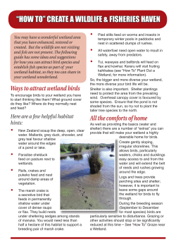


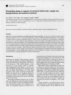
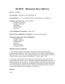


© Copyright 2026