1. business and industrial
2. energy
3. nuclear power

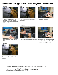
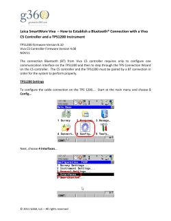
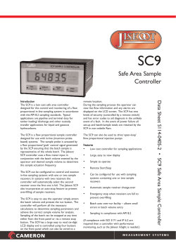
PACKED BED REACTOR
OPERATING MANUAL
REVISION: FALL 2014 – C
EDITOR: HAROLD J. TOUPS
INTRODUCTION
The study of reaction kinetics is at the heart of chemical engineering. Coupled with separations
(i.e., mass transfer) and process control, these three elements are chief distinguishing
characteristics separating chemical engineering from, say, mechanical engineering. Similarly,
knowledge and skill in these three disciplines distinguish chemical engineers from the rest of
engineers.
Laboratory and pilot scale experiments in kinetics – properly performed – provide the necessary
data and insights needed to understand reaction mechanisms; evaluate the effects of
composition, temperature, and catalysts on the rates of reaction; and ultimately allow chemical
engineers to design commercial scale reactors for the manufacture of valuable products.
BACKGROUND ON THE ETHYLENE HYDROGENATION REACTION
The hydrogenation of C2H4 has been studied as a model reduction reaction in characterizing
new metal catalysts. Beeck, in 1950, was one of the first to systematically study the reaction[1].
He found that nickel, while not the most active metal catalyst for this reaction, is active enough
that the hydrogenation reaction can take place at < 200°C.
A S
H 2  2S
AS
HS  HS
Section: Introduction
The reaction typically involves adsorbed, dissociated H2 reacting with adsorbed C2H4. In other
words, both hydrogen atoms and C2H4 molecules form bonds with a metal site (here denoted as
S). The strong bonding of C2H4 with S weakens the double bond sufficiently to allow hydrogen
atoms to add to C2H4, forming ethane, which is not adsorbed. A mechanism for the reaction has
been suggested by Butt (letting A = C2H4, E = C2H6 and S = a metal site) and can be written as
follows[2]:
(1)
(2)
1
AS  HS 
 AHS  S
(3)
AHS  HS 
E  S  S
(4)
If we assume the third reaction is the rate-limiting step, and that the total amount of S sites is
constant (So) we can use an approximate mass balance:
(S0 )  (S )  ( AS )  ( HS ),
(5)
and the quasi-equilibrium assumption of the first two reaction steps to obtain a theoretical
kinetics expression:
r  k ( H 2 )1/2 ( A)(S0 )2 [1  K1 ( A)  K21/2 ( H 2 )1/2 ]2
(6)
Note that in the approximate mass balance we assume that
(S ), ( HS ) and ( AS )
( AHS )
(7)
Also note that (So) is a constant as long as the total number of metal sites remains the same.
When the number of metal sites decreases with respect to time, we say the catalyst
deactivates; when it increases, the catalyst activates. In this reaction, deactivation can be
caused by a side reaction with this stoichiometry:
aC2 H 4 
(CH )2 a  aH 2
(8)
Section: Background on the Ethylene Hydrogenation Reaction
The component (CH)2a – called coke – is too heavy (i.e., a is large) to desorb from the metal
sites and so these metal sites are effectively removed from the catalysis[3]. However,
subsequent reaction conditions may cause the coke to break down, in effect re-activating the
catalyst.
For the kinetics described above, it is evident that for low concentrations of C2H4 the rate is
first-order in C2H4 while for high concentrations of C2H4 it is -1 order. Rate expressions of this
type –also common in enzyme-catalyzed reactions – are called Langmuir-Hinshelwood rate
expressions. Since the equilibrium constant K1 is temperature-dependent, this rate expression
tells us that the order m for C2H4 in a power law rate expression of the type
r  k ( A)m ( H 2 )n
(9)
will change with temperature. Most rate expressions regressed from experimental data are of
the power law type.
The catalyst used in the packed bed reactor employs Ni as the active component, but contains
SiO2 in significant quantity as well. The SiO2 serves as a support for the Ni; its only purpose is to
provide a large surface area for the Ni to cover. The SiO2 is chemically inert at the conditions
used here. Another inert material, SiC, is used to fill up the rest of the reactor.
General reaction kinetics references abound. Fogler’s book is particularly good[4].
2
PACKED BED REACTOR – EXXON CATALYTIC REACTOR PILOT UNIT
Section: Packed Bed Reactor – Exxon Catalytic Reactor Pilot Unit
Donated by the former Exxon Research and Development Laboratories here in Baton Rouge,
the CAT unit – as it is sometimes called – is capable of many different catalyst experimental
testing strategies. Currently, it is equipped to facilitate heterogeneous packed bed reactor
studies testing nickel and other metal-on-support hydrogenation catalysts in the hydrogenation
of ethylene – C2H4. Figure 1 is a simplified schematic of the reactor system.
Figure 1 – Exxon Catalytic Reactor Pilot Unit schematic.
The reactor itself (detailed in Figure 2) is a steel tube contained within a sandbath. The
sandbath is fluidized using air and is heated by metal resistance heaters. Large quantities of
heat can be transferred rapidly to this pilot plant reactor. Catalyst cylinders are located in a
narrow layer at a point roughly 4 inches above the lowest movable thermocouple position. The
precise location and extent can be determined by detection of the reaction exotherm (see
Longitudinal Temperature Variation section later in this document).
Precautions have been taken to make this a safe system. There are relief valves on the system,
a high temperature shutdown, and only diluted H2 (see the specification information on/next to
the cylinder) is used. However, with any reacting system, strict adherence to safety procedures
3
is necessary. The lower flammability limit of H2 in air is 4 vol. %[5], therefore it is important to
ensure that the reactor is not leaking H2 into the surrounding sandbath.
Section: Packed Bed Reactor – Exxon Catalytic Reactor Pilot Unit
Key measurement components of this pilot unit are instrumented through the Emerson Process
Management DeltaVTM control system.
Figure 2 – Reactor mechanical drawing denoting thermowells and inlet preheat coil.
4
OPERATING INSTRUCTIONS
The following section is devoted to instructions on the typical operation of the pilot unit as
currently configured.
LOGGING INTO AND USING THE DELTAV™ SYSTEM
The DeltaV system can be accessed in virtual fashion from any of the computers in the control
room. Though there are several DeltaV virtual machines that allow such access, the che-uolabdv3 virtual machine is reserved for, and set up properly for access to the CAT Unit. Accessing
this virtual machine is done through VMware’s Horizon View Client, as outlined in the multistep
process given below.
To access the che-uolab-dv3.lsu.edu DeltaV virtual machine, follow the steps outlined here:
Section: Operating Instructions
1. Logon to Windows 7 using a valid LSU ID and password
2. Double-click the VM Horizon View Client icon on the Desktop. The app will open and
a screen such as that show in the figure below will appear:
3. If an icon for che-uolab-dv3.lsu.edu is already showing in the gray area, skip to Step
8 in this process. If NO icon for che-uolab-dv3.lsu.edu is showing in the gray area (as
depicted in the figure above), then double-click the Add Server icon. A new popup
will appear, as shown in the figure below:
5
Section: Operating Instructions
4. Here, enter the desired server’s name: che-uolab-dv3.lsu.edu and click the Connect
button. At this point, another popup will appear; one that looks like the following
figure:
5. Here, enter administrator as the User name and deltav as the Password. Click the
Login button.
6. The dv3 virtual machine should appear next and another DeltaV Logon menu
displays. Type deltav in the Password: field. Click OK.
7. A Flexlock menu window appears next. Click the Windows Desktop button.
Minimize this menu window. At this point, skip to Step 13.
8. You are here because an icon for che-uolab-dv3.lsu.edu is showing in the gray area,
appearing like that show in the figure below:
6
Section: Operating Instructions
9. Double-click the che-uolab-dv3.lsu.edu icon, at which point the following popup will
appear:
10. Here, the proper User name has already been loaded but you must enter deltav in
the Password field. Click the Login button.
7
11. The dv3 virtual machine should appear next and another DeltaV Logon menu
displays. Type deltav in the Password: field. Click OK.
12. A Flexlock menu window appears next. Click the Windows Desktop button.
Minimize this menu window.
13. You have logged in successfully to the che-uolab-dv3.lsu.edu virtual machine.
At this point, the DeltaV virtualized station of choice is up and operating. From here you can
access the DeltaV Operate Run program and the Process History View program (and Control
Studio from che-uolab-dv1) from the Windows Start menu. You should also be able to access
the apps drive and a connected jump drive (if installed) from Windows Explorer on the DeltaV
virtual machine.
To start up the control schematic navigate to Start > DeltaV > Operator > DeltaV
Operate Run. The UOLAB_Overview display should come up. Click on the hot-linked
photo of the Exxon Catalytic Reactor unit. Doing this should automatically open the CAT1
display. If a dialog box appears indicating an error, click Skip All on the dialog box.
CHANGING CONTROLLER PARAMETERS FROM CONTROLLER FACEPLATES
On the larger operations schematic, the appearance of a small icon – identifiable by a gray box
with three vertical lines – signals the presence of an automatic controller. To the left of each
controller icon are the process value (PV, the measurement) in yellow, the setpoint (SP) in
white, and the output (OP) in cyan. To change a parameter on a controller, click on this icon to
bring up a faceplate. From the faceplate, controller mode can be changed by clicking on the
desired mode button on the left side of the faceplate.
Section: Operating Instructions
Manually changing the controller output (OP) is only possible in MANual mode. To change the
controller output, click on the MANual value field at the top of the faceplate and enter a new
value. Click-dragging the large cyan pointer – present only when the controller is in MANual
mode – to a new position also changes the output of the controller. The smaller cyan pointers
are output limit indicators and cannot be changed from the controller faceplate.
When the mode is not MAN, the controller uses the process value (PV), setpoint (SP) and
tuning constants to calculate a new output (OP) every processing pass.
Manually changing the controller setpoint (SP) is only possible in AUTO mode. To change the
controller setpoint, click on the setpoint value field on the right side of the faceplate and enter
a new value. Click-dragging the large white pointer – present ONLY when the controller is in
AUTO – to a new position also changes the setpoint of the controller. The smaller white
pointers setpoint limit indicators and cannot be changed from the controller faceplate.
8
ACCESSING ADDITIONAL CONTROLLER DETAILS
Across the bottom of the faceplate are six icons that call up other displays with more details
about this controller. The two most useful ones for this experiment are the first one from the
left, which provides access to controller parameters; and the second one from the right, which
calls up the historical trend for this controller.
ACCESSING REAL-TIME PROCESS HISTORY
To start up the real-time process history view at any time, simply navigate to Start >
DeltaV
>
Operator
>
Process
History
View, and then open
CATUnitOverview (if it does not open automatically). Chart scales can be compressed or
expanded by clicking those buttons on the menu bar. Scales can be shifted up or down by click
dragging on the scale of interest.
STARTUP
1. Be certain the air to the sandbath is on. The rotameter should read ≈ 5 or higher and be
held constant from run to run to provide consistent heating.
2. Enable main power to the sandbath heater by pushing the black-colored START button
on the CAT unit’s panel board.
3. Set automatic temperature controller (TIC-10, for the sandbath) to desired initial set
point, if the reactor is to be heated.
Set mode to AUTO unless you know the exact output desired.
(You can also turn auxiliary heater on (output ≤ 90%) if you desire a rapid heatup, but be
sure to it turn off when the skin (heater) temperature nears your desired reactor T; the
auxiliary heater is not controlled at this time and cooling (≈10 °C/hr) takes much longer
than heating.) – Not typically recommended – See Instructor for guidance.
Section: Operating Instructions
The reactor temperature can lag the heater temperature significantly. You may want to
change the selector switch for TIC-10 to the skin thermocouple (this tells the controller
to use the skin T/C as its input), and raise the set point to compensate for the difference
in temperature between skin and reactor temperature (anywhere from 2 to 5°C is
typically, depending on the desired reactor temperature). You can also change the
selector switch later.
The highest temperature to be used in any experiment is 200oC. The DeltaVTM computer
has been programmed to reduce the input heating power by half at 200oC and to shut
off the heaters at 220oC. A "CRITICAL" warning light will alert you to the high
temperature. Both the sandbath and reactor temperatures are monitored, and both are
programmed to alarm and shut off the heaters.
9
4. Be sure the breaker for the sandbath main heater (#10) is on, as well as breakers for
instrument power (#4), tape heater and GC (#5), and control (#7).
5. If the ammeter for the sandbath heaters is not showing current, press the START switch.
Steps 1 through 5 can be rapidly performed the morning of the experiment. Then you can leave
the experiment unattended with NO GAS FLOWS (unless otherwise negotiated with your
instructor). The catalyst is stable in a no flow condition and, most typically, you can start the
flows during the normal afternoon lab period.
Special Item:
If experimental guidance from your instructor calls for, or you believe you will need to and have
obtained permission to introduce gas flows AND leave the unit unattended during the morning
of an experiment, complete and post the Unattended Operations Placard provided in the
Appendix of this manual, following the instructions given therein.
Do NOT leave the reactor unattended AND at elevated pressure. Use 0 psig during the
pretreating period.
The temperatures can be monitored on the control schematic chart or – even better – using
Process History View. The reactor effluent flow rate should be checked periodically. If
problems (loss of flow, runaway temperature) develop, SHUT OFF BOTH REACTANT FLOWS
USING APPROPRIATE SHUTOFF VALVES AND TURN ALL HEATERS OFF. LEAVE SANDBATH AIR ON.
Should the experimental program suggest or call for the use of elevated pressure reaction
conditions, this can be accomplished by loading the dome of the reactor back pressure
regulator (V-8) with nitrogen pressure. Unless otherwise advised by your instructor, limit
reactor pressures to 30 psig. (Note: Tests in the fall of 2009 indicated that the flow meters
yield the same flow calibration at elevated pressure that they do at 0 psig.)
SETTING FLOW RATES
Set flow rates prior to turning on heaters on Day 1. Note that the main operating screen has a
digital value designating whether the computer or the panel board will be used for this. Set this
value to 1 for computer use. The H2/N2 mixture is set first, using mass flow controller FIC-301.
FIC-301 is a linear response device, but only operates between roughly 20% and 100% of rated
flow. To minimize uncertainty in rate and other calculations which may be based on this flow
rate, a precise calibration of this meter is needed, relating raw input (Field Value % in DeltaVTM
terminology) to the actual flow as measured by the soap bubble-o-meter.
Section: Operating Instructions
The reactor temperature will typically show some oscillation around the controller set point.
This is normal. However, it is not normal for the sandbath T’s to greatly exceed the reactor
temperature by more than 10 °C after a prolonged period. This condition may indicate a
blocked filter on top of the sandbath. Remove and clean it; you can do this while the unit is
running.
10
To build this calibration, a) Bypass the reactor; and b) Determine the flow rates over a range of
field value, or output, percent by changing the controller’s valve opening in MAN (manual)
mode. Wait a minute prior to taking readings to ensure that a steady flow is achieved. The
results from this work can be used as a stand-alone calibration for FIC-301 and, if desired, the
linear calibration coefficients can be entered into the DeltaVTM system to avoid the need for the
stand-alone tool. If the calculated zero (0% of input) is far from zero flow and/or the calibrated
span (100% of input) is far from the estimated maximum flow rate of this meter, there may be a
problem with the instrument requiring the attention of the Lab Coordinator. When finished
checking this flow meter calibration, re-route flow through the reactor. Check a flow rate again
at a high output %. It should be close to your previous reading; if well below (say > 10%), there
may be a serious leak in the reactor; notify the Lab Coordinator.
Calibrate the ethylene mass flow controller, FIC-302, in a similar manner by bypassing the
reactor again, and shutting off the N2/H2 flow. Be sure to close the shutoff valve just before the
mixing tee. Set C2H4 flow rates using FIC-302 in MAN mode. This is also a linear response
device, but it too only operates between roughly 20% and 100% of rated flow. Again use the
bubble-o-meter to determine (using two or more points along the span) the calibration slope
between flow rate and input (Field Value %), and then the calculated zero and span.
To start a reaction, route (or re-route) the combined H2/N2 mixture and C2H4 flows to the
reactor.
If the chromatographic method in use is capable of total feed analysis, it is probably wise to
take at least one sample with the feed through the bypass (a blank sample) to determine the
feed composition. It's OK to change flow rates on the fly without bypassing the reactor. Again, if
GC method allows for it, you can verify that your gas chromatograph is set-up properly by
running the H2/N2 and C2H4 separately, and checking the results versus the composition noted
on the cylinder labels.
Special Item:
LONGITUDINAL TEMPERATURE VARIATION
As conversion of ethylene increases, even the small quantity of catalyst and the large amount of
carborundum diluent present in the reactor may not prevent a longitudinal increase in
temperature from occurring, resulting in a non-isothermal kinetic impact on reaction rate. If
this is of consequence to your experimental program, the longitudinal temperature variation
can be measured and its effect accounted for in post-run analysis.
The following steps illustrate how to measure longitudinal temperature variation whilst carrying
out the ethylene conversion reaction:
Section: Operating Instructions
N.B.: When either calibrating meters or checking exit flow rate during reaction – indeed,
anytime the bubble-o-meter is being actively used to measure flow – the Agilent GC sample line
should be blocked out. This must be done to avoid having gases from the GC contribute
erroneously to measured flow rate through the bubble-o-meter.
11
1. With the reactor thermocouple bottomed-out to its full extent in the reactor centerline
thermowell, collect sufficient data (using the method outlined later in this manual) to
identify an average temperature from this thermocouple.
Note: If a sandbath or skin couple is being used for control, the reactor couple can be
moved with impunity. If, however, the reactor thermocouple is being used to control
temperature, then moving the reactor couple will affect temperature control
undesirably. To avoid this, temporarily place the temperature controller in MANual
mode while performing this procedure, returning it to AUTO mode after completion of
the procedure.
2. Lifting this thermocouple a small and known distance up, again collect sufficient data to
identify an average temperature from this thermocouple. As the couple may be hot, use
appropriate gloves or a cloth to protect your fingers from the lower portion of the
couple (see Mr. Perkins for any needed materials).
3. Repeat step 2 until the thermocouple no longer shows a rise in reactor temperature. A
chart of these average values will reveal the start and end of the catalyst bed
temperature rise, as well as the quantitative data necessary to deal with longitudinal
temperature variation resulting from this exothermic reaction.
4. After gathering all necessary data, return the reactor thermocouple to its bottomed-out
position, being careful to guide the couple down without crimping it. As the couple may
be hot, use appropriate gloves or a cloth to protect your fingers from the lower portion
of the couple (see Mr. Perkins for any needed materials).
CHROMATOGRAPH OPERATING INSTRUCTIONS (AGILENT 3000A MICRO GC)
USING THE AGILENT 3000A
1. Check to make sure the carrier gases (i.e., helium and argon cylinders located behind
the GC itself) are open to the GC and that pressure levels are sufficiently high (i.e.,
supply pressures of roughly 80-to-90 psig and cylinder pressures of 200+ psig). If the
levels look low, contact the Lab Coordinator.
2. Check to ensure the direct connect tubing line to the GC is connected to the source to
be analyzed; i.e., the standard gas cylinder if performing a calibration or the CAT unit
itself if analyzing process gas. If this tubing line needs to be moved from one source to
the other, contact the Lab Coordinator.
3. Log into a suitable UO Lab Control Room computer using your LSU ID and password.
4. Open the Remote Desktop Connection application. In the destination line, type the
virtual computer’s name: che-uolab-gc3. Hit Enter on the keyboard. You will be asked to
Section: Operating Instructions
Use of the Agilent 3000A Micro GC requires the following: a) the GC is powered up and on, b)
carrier gases are available and aligned, c) the gas source to be analyzed is aligned, and d)
software to operate the GC and analyze results is accessible. Instructions for meeting these
requirement are outlined below.
12
log in again, using your LSU ID and password. This will take you to the che-uolab-gc3
virtual computer desktop.
5. On the desktop of that virtual computer, click on the icon for MicroGC 3000 (online), as
shown in the image below:
9. Performing an analysis:
a. When you are ready to perform a run, click on Control (same top line as File) and
then Single Run. A popup menu will appear.
Section: Operating Instructions
This will open the GC operating and analysis software application.
6. At this point you will see a navigation window, a top menu with icon buttons, and a grey
primary screen.
7. Load the method “PH-CAT4”. To do so, click File → Open → Method and choose the
method titled “PH-CAT4”. The method is now loaded onto the system and ready to be
used. The method name should be displayed at the very top of the window. It may be
loaded already; check the top line of the MicroGC program to see if it is already enabled.
8. Display the Instrument Status by clicking on Control → Instrument Status. It may take
some time for the method settings to equilibrate the GC. You cannot perform a run until
all parameters in Instrument Status are green (even though we are not using Channels C
or D).
13
b. Your run will need both a Sample ID as well as a Result Name (group name or
name and run number and date-time, for example). Once you have those lines
complete, click Start in the popup window. Four plots will pop up (one for each
detector).
c. It may take a minute or two for the software to begin plotting. You will know
that the run setup was successful by the changing of the status bar (bottom
right-hand corner) from green to blue.
Section: Operating Instructions
10. For the compounds being tested, your results will come from Channel A and Channel B.
Hydrogen and nitrogen will be detected on channel A, while methane, ethane, and
ethylene will be detected on channel B.
11. To view the report for your run, click Reports → View → Normalization. A report with
the known compounds will pop up.
14
12. If prompted to save Method, click NO. Clicking Yes would create a new method file and
could potentially change the CAT-PH settings.
13. When finished with the GC, log out of the Remote Desktop Connection application using
the Start menu (do NOT exit via the X at the top of the blue Remote Desktop Connection
bar). Logging off not using the Start button would leave you logged into che-uolab-gc3,
preventing the other groups/instructors from logging in.
14. Leave the carrier gases on.
15. When completely finished (both the GC and DeltaV), log off of the main desktop via the
Start button again.
REACTOR SHUTDOWN
The following steps constitute a safe and orderly shutdown of the Exxon Catalytic Reactor Unit:
1. Shutdown main power to the sandbath heater by pushing the red EMERG. STOP button
on the CAT unit’s panel board.
2. Set automatic controller temperature to 0ºC (AUTO) or 0% output (MAN).
3. Set auxiliary heater output to 0%, if on.
4. Set C2H4 flow to 0%.
5. Shut off C2H4 block valve at the mixing tee.
6. Shut off C2H4 main cylinder valve.
7. Shut off air flow to fluidized bed.
8. Wait ~ 2 minutes; then shut off H2/N2 mixture flow to the reactor by setting flow to 0%.
(Maintaining flow for those 2 minutes leaves a blanket of this mixture in the reactor,
prolonging the life of the catalyst.)
9. Shut off H2/N2 mixture main cylinder valve.
11. All other valves should be left open.
EMERGENCY HEATER SHUTDOWN
If the reactor heater needs to be shut down under emergency conditions, press the red
Emergency Stop (EMERG. STOP) button on the front panel of the unit IF CONDITIONS PERMIT
THIS TO BE DONE SAFELY.
Section: Operating Instructions
10. Shut off N2 cylinder main cylinder valve, if open; then, relieve pressure on the reactor
back pressure regulator IF it has been set above 0 psig.
15
HISTORICAL DATA ACCESS USING DELTAV CONT INUOUS HISTORIAN
A continuous historical record of all relevant temperatures, flows, and levels is kept by the
DeltaV system on its hard disk(s). Selected portions of these data can be imported into an Excel
spreadsheet for analysis. This spreadsheet must be saved to a flash drive or a personal directory
if it is to be used on any other personal computer than a dedicated DeltaV workstation as files
stored on the DeltaV network are not accessible from the general LSU network.
To import data from DeltaV history to Excel, Emerson has provided an Excel add-in called the
DeltaV Continuous Historian. It appears under the Add-Ins menu in Excel 2007
when this program is opened on a DeltaV workstation. Any process variable that is enabled in
History Collection can be imported. Most of these variables are collected every 10
seconds, 30 seconds, or 1 minute, so it doesn't make sense to try to read the data any faster.
Though the menu features of the DeltaV Continuous Historian can be used for their
intended purpose, requesting an ad hoc retrieval of data for more than one or two tags is
tedious and time-consuming. To avoid this labor, an Excel 2007 template file is available for
TDU data retrieval. This template is preloaded to request ALL the historically trended TDU tags.
The only information that the user must supply is the starting date and time, the ending date
and time, and the time interval between data values.
To import data, open Excel 2010 on the DeltaV workstation and follow these steps:
1. Put Excel calculations in Manual mode before opening the template or attempting to
change the starting and ending dates.
2. Open the data retrieval template file for CAT.
It is located on the Desktop, in the DeltaV_Excel_Data_Collector_Files folder under the
name CAT_Data_Retrieval.xlsx
For example, data starting October 5th, 2011 at 9AM would be entered as 10/5/2011
9:00
4. Enter (or modify) the ending date and time for the data of interest as mm/dd/yyyy
hh:mm into cell A6.
For example, data ending October 5th, 2011 at 3PM would be entered as 10/5/2011
3:00PM or 10/5/2011 15:00
5. Enter (or modify) the desired time interval between data values.
Section: Operating Instructions
3. Enter (or modify) the starting date and time for the data of interest as mm/dd/yyyy
hh:mm into cell A4.
16
For example, to request data values every 10 seconds, enter =”10seconds” into cell A8.
For data values every 2 minutes, enter =”2minutes” into cell A8. Any value of seconds,
minutes, or hours may be used, but some values make more sense than others. Using
values faster than the fastest data originally collected makes no sense. So, values below
10 seconds only make sense if data collection on some variables has been set to time
intervals below 10 seconds. Data will be interpolated where there are no values.
A maximum of 2161 readings (2160 intervals) are available in any one data retrieval
operation. This will allow the retrieval of 6 hours of 10 second data, 36 hours of 1
minute data, or any other combination that results in 2160 (or fewer) intervals. If more
data are required, two separate requests must be made and concatenated manually. Of
course, if only a few tags are needed, one can bypass the use of the template and
retrieve data ad hoc using DeltaV features.
6. After entering the last of these user inputs, click the Add-Ins menu tab, click the DeltaV
drop-down tab, roll over the Continuous Historian option, and select Refresh. All values
in the spreadsheet should update, signaling successful retrieval of data.
Select the entire worksheet (by clicking in the upper left hand corner of the worksheet
adjacent to the A1 cell. Copy this selection (e.g., ctrl-c). Select the 2nd worksheet tab.
Using Paste Values, paste the values copied from the Data Collection tab into the 2nd
worksheet. These values are now static and will be available even when the spreadsheet
is relocated to another computer. The values in the first tab can be deleted at this point
IF the file will not be used to retrieve additional data from the DeltaV.
8. Save this file with an appropriate name to a device or drive separate from the DeltaV for
use at a later time. (Remember that calculation mode for that file is Manual.)
9. The units for the data are the same as in DeltaV. If the word shutdown appears instead,
then either:



History collection was not enabled for that variable, or
No history collection because the system was shut down, or
No history collection because the variable did not change more than its deviation
value set in history collection (i.e., nothing's changing!)
PROCESS CONTROL BACKGROUND AND THE DELTAV SYSTEM
The control of reaction processes is critical in the chemical, polymer, pharmaceutical,
electronics, and food processing industries. The control problems can be difficult due to the
different demands the reaction imposes on the process – rapid startups and shutdowns,
Section: Process Control Background and the DeltaV System
7. To save these results, these data must be turned into static values, as follows:
17
possible runaway temperature, narrow operating range, etc. Also, it may be difficult to
determine optimal control parameters for any control loop, because different operations may
require markedly different control strategies. Equally important is the setting of operator
alarms and interlocks (an interlock is a logical statement which, when true, locks out the
operation of specified equipment). The logic involved in such operations can be complex even
for simple units.
For the catalytic reactor, you may also be assigned a study of its control/operations
programming in order to make improvements to the control system. The control platform is
DeltaVTM, an Emerson Process Management system that is compatible with several ISA
Instrument Society of America) protocols. It is a modular system; i.e., modules built in a
program called “Control Studio” perform different types of tasks. The main programs and the
modules that have been constructed are listed below:
Control Studio – creates control loop and sequential function chart modules. A sequential
function chart (SFC) is a set of commands for performing a subset of plant operations in a
sequence.
Operate (Configure) – creates process and instrumentation diagrams (P&IDs), with special links
for operation of equipment and control loops
Operate (Run) – general plant operations – setting basic control loop parameters, starting
sequential function charts, directly operating equipment from the P&IDs.
Process History View – examines historical data graphically, if the system has been programmed
to record such data.
The operation of Operate (Run) and Process History View will be demonstrated by the
instructor. The other three programs are for configuration only; you will not need them to
operate the system and they are not available on the computer near the experiment.
Instructions for retrieving data from the control system into Excel are given in “retrievedata.txt”
(in d:\uolab). There are extensive on-line instructional manuals and help files (right click usually
gives you a choice for help) to aid in understanding how to use DeltaVTM. Basically, if you are
familiar with VBA, or any other object-oriented programming language, then you already
understand a lot about Control Studio. If you are familiar with Windows-based drawing
programs, you could pick up Operate (Configure) easily. If you are not familiar with these, you
may consider going back to the 19th century.
The only schematic now provided is CAT1. Start the program DeltaVTM Operate. Open the file
CAT1. Now let’s work with CAT1. You see icons that can be operated in the schematic. For
example, you can click on a faceplate and get the temperature controller TIC-10. This is a PID
controller manipulating the main heater output (OUT) in order to control reactor T. The reactor
T is the measured (process) variable, PV. However, you can click on the input TSELEC and
change the PV that the controller uses. Leaving this loop in manual, you can increase the output
of the heater from 0 to 100% (use the left control). You see the measured variable in the right
indicator. There is also an input box for the set point (SP) – the desired process variable value
Section: Process Control Background and the DeltaV System
Explorer - configure the system, including the I/O.
18
when the controller is in AUTO. Set OUT back to 0%; change to AUTO; and try a SP of 80°C. You
should see OUT gradually increase. Clicking on the bottom left icon gives you the module detail
which contains parameters you would need to tune a controller. Such tuning can be done either
here or in Control Studio. However, Control Studio can only be opened with write access on the
DV1 console (or the DeltaV server itself).
Now examine a control module in Control Studio on a console with write access. Open the
DeltaVTM Explorer, select module TIC-10 in area CAT, and open it in Control Studio. This module
contains the temperature controller, the analog output devices (heaters) and analog input
devices (thermocouples). This will allow you to operate this subsystem from Control Studio.
Click on menu item “VIEW” then “ONLINE”. You will see numbers appear on the screen – you
are operating the entire module in real time. Click on the PID1 box. This also gives you access to
the controller. Set “OUT” to 30% using the “Parameter List” in the bottom left corner. This will
set the main heater output to 30%, if some conditions are met. Following the arrows (logic
flow), determine what these conditions are (click in the appropriate boxes; then click on
“Expressions”). Conditional expressions are logical statement(s) which must be satisfied before
the program performs a subsequent action. Expressions evaluate as 0 = false, 1 = true.
This completes a brief tour of DeltaVTM. In order to complete your assignment you will have to
learn how to use Operate (Run) and Process History View. If problems, you can consult the
Books Online and the extensive online Help files. However, any direct question on a particular
topic will be answered. Some additional information on process control background is provided
below; if you have already completed a process control lab, you can probably skip this
information. Equipment specifications are in the figures below.
The reaction system is equipped with thermocouples, gauge pressure transmitters, thyristors
(also called SCRs, these are power controllers) for the heaters, electronic flow control valves,
and a motor controller for the recycle pump. The following is some background on the
operation of such instruments and their control. For more detailed descriptions you can read
Ch. 8 and 9 of Process Dynamics and Control by Seborg et al. or Ch. 5 of Smith & Corripio,
Principles and Practice of Automatic Process Control, or a similar book on process
instrumentation and control.
Sensor/Transmitter: An example differential pressure transmitter is the one installed to
measure the level in the reactor. The transmitter sends an electric signal in the range of 4 to 20
mA (converted to 1-5 V by a resistor) to the controller; this signal is proportional to the level in
the tank. The controller converts this signal into a percent of range reading according to the
following formula:
PV  100 
(h  h0 )
hs
(10)
Section: Process Control Background and the DeltaV System
Similarly, open FIC-301B in Control Studio. This contains the transmitter and controller for N2/H2
flow. Locate where the zero and span for the transmitter output would be set. Examine which
alarms have been configured, and how they have been configured.
19
where PV is the process variable (level) in percent of transmitter range, h is the level, h0 is the
zero of the transmitter range (lowest level that it can measure), hs is the span of the transmitter
range, that is, the difference between the maximum measurable level and the zero level. The
DeltaVTM controller can then convert this reading into any engineering unit desired – this is
done in Control Studio.
Power Controllers and Control Valves: The controller outputs (AOs) are transmitted as 4 to 20
mA corresponding to 0-100% range. When a control valve is actuated by air pressure, a currentto-pressure (I/P) transducer is used to convert the current signal into air pressure (3-15 psig
range). The control valve can be air-to-open (fails closed), i.e., it opens as the controller output
signal increases; it can also be air-to-close, which is just the opposite. The flow through a
control valve is usually measured by a d/p transmitter (with orifice), a turbine meter, a Coriolis
(spiral tube) flow meter, or the resistance of a heated metal filament (anemometer). In this
experiment, electronic controllers with anemometer flow sensors are used.
An important characteristic of a feedback controller is the direction of its action, i.e., which way
should it change its output when the measured variable rises. If an increase in the output signal
opens a valve on the inlet flow to a tank, which way should the controller output to the valve
actuator move (increase or decrease) when the tank level (measured variable) rises? If your
answer is "increase" we would have a direct acting controller, and if your answer is "decrease",
it would be a reverse acting controller. Which action is correct for the controller in TIC-10?
Why?
The controller calculates the error or difference between the SP and the PV:
E  SP  PV
(11)
The ideal PID controller output signal is given by:
OUT  OUT0  Kc  [ E 
1
dE
Edt  Td
]

Ti
dt
(12)
where the controller output in the range of 0 to 100%, OUT0 is the initial (time zero) output,
and KC, Ti, and Td, are, respectively, the proportional gain, reset (or integral) time, and rate (or
derivative) time. These adjustable parameters can be set on the controller using the module,
either in Control Studio or Operator Interface. Real PID controllers are more complex, but the
above is a useful approximate model.
The three terms in the bracket of the equation represent the proportional (P), integral (I), and
derivative (D) modes of the feedback controller (PID). As you can see, the proportional term
makes the controller output proportional to the error and acts immediately upon a change in
the process variable or in the set point. The second term, integral, is slower because it acts over
time; its purpose is to force the error to zero. The derivative term acts on the rate of change of
Section: Process Control Background and the DeltaV System
Feedback Controllers: These regulate a measured process variable (e.g., temperature) by
adjusting an OUT signal to vary a manipulated variable (e.g., power output). Control is
accomplished by adjusting the SP of the controller (e.g., TIC-10 in Operator Interface), and by
changing the mode of the controller to AUTO.
20
the error; it is the fastest of the three terms. Flow rate controllers usually do not require the
derivative term, so Td may be set to zero for these.
TUNING CONTROLLERS
Figure 3. Controller tuning map for tuning of PI controllers. All subplots are the response of
PV versus time after step change in set point. (Practical Process Control by Cooper, 2004)
There are two general approaches to controller tuning: trial-and-error and model-based (an
approach covered extensively in ChE 4198 – Process Control). Because flow rate dynamics are
relatively fast, a trial-and-error method is preferable in establishing optimal Kc and Ti for flow
rate loops. But for the more complex loops controlling temperature or pressure, model-based
approaches are preferred. A standard model for the open-loop (controller in MANUAL mode)
Section: Process Control Background and the DeltaV System
Consider a simple flow controller. The position of a flow control valve or a variable pump speed
is the manipulated or controller output, and the flow rate is the measured or process variable.
The adjustment of the controller parameters to obtain a fast stable response of the variable
being variable is known as tuning the controller. Figure 3 (Controller Tuning Map) shows,
qualitatively, criteria for evaluating controller performance. The “detail” screen of the module
faceplate in Operator Interface would be used to enter candidate Kc, Ti and Td values, as well as
other controller parameters.
21
dynamics of many systems is first-order-plus-dead-time, or FOPDT. The open-loop dynamics are
assumed to follow the form (when put into dimensionless form):

dY
 Y  K  X  H (t   )
dt
(13)
The measured variable is Y (dimensionless, measured as fraction of span), the output or
disturbance variable is X (dimensionless, same units) and the H-operator is the unit step
function, which models the pure time delay of the process. The adjustable parameters are the
steady-state gain (K), the system time constant (), and the time delay (). Normally, a test of
the system in open-loop is performed as follows. The system is allowed to come to a steady
state, then a disturbance is introduced (X = M). A plot of Y vs. t is constructed – known as a
process reaction curve – and from this, values of K, , and are estimated, from which
candidate Kc, Ti and Td values of the controller parameters can then be generated.
Estimating the process characterization parameters (K, , and ) can be as simple as using
graphical interpretation of the resulting process reaction curve (e.g., the Cohen-Coon open-loop
method[6]) or as complex as performing an optimization procedure to minimize the error
between the entire set of process reaction curve data and the presumed first-order-plus-deadtime model[7].
Candidate tuning parameters are then estimated using an appropriate choice from the myriad
methods available, such as Direct Synthesis (DS)[8], Internal Model Control (IMC)[9], and
Cohen-Coon (CC)[6].
[1]
O. Beeck, "Hydrogenation catalysts," Discussions of the Faraday Society, vol. 8, pp. 118128, 1950.
[2]
J. B. Butt, "Progress toward the a priori determination of catalytic properties," AIChE
Journal, vol. 22, pp. 1-26, 1976.
[3]
J. B. Peri, "Infra-red studies of carbon monoxide and hydrocarbons adsorbed on silicasupported nickel," Discussions of the Faraday Society, vol. 41, pp. 121-134, 1966.
[4]
H. S. Fogler, Elements of chemical reaction engineering, 4th ed. Upper Saddle River, NJ:
Prentice Hall PTR, 2006.
[5]
(2005, August 18, 2010). Lees' Loss Prevention in the Process Industries: Hazard
Identification, Assessment and Control (3rd ed.).
[6]
J. A. Romagnoli and A. Palazoglu, Introduction to Process Control. Boca Raton: Taylor &
Francis, 2006.
[7]
D. J. Cooper. (2008, August 18). Modeling Gravity Drained Tanks Data Using Software.
Section: References
REFERENCES
22
[8]
D. A. Mellencamp, et al. (August 18). Process Dynamics and Control, Chapter 12 slides.
Available: http://www.che.utexas.edu/course/che360/lecture_notes/chapter_12.ppt
[9]
D. A. Cooper. (2006, August 18). PID Control of the Heat Exchanger.
APPENDIX
Section: Appendix
Unattended Operations Placard (See next page.)
23
Exxon Catalytic Reactor Unattended Operations
Unattended Use1 by: ______________ between _______ and2 _______ on __________
Hydrogen/Nitrogen Flow Rate (cc/min): _______________________________________
Ethylene Flow Rate (cc/min): ________________________________________________
Heating to Reactor Temperature, °C ____________ Pressure, psig __________________
Email Notification to Lab Coordinator ([email protected]) at: _________ (clock time)
If necessary, hydrogen/nitrogen flow can be stopped immediately by
blocking out the supply cylinder behind the unit. It is the far right
cylinder as you face the back of the unit. Simply turn the main cylinder
valve clockwise until closed.
1
2
If necessary, ethylene flow can be stopped immediately by blocking out
the supply cylinder at floor level on the unit skid’s left side. It is the only
cylinder at that location. Simply turn the main cylinder valve clockwise
until closed.
Hang this form on the reactor sandbath after completing accurately with needed information. Make sure that the exit gas valve is directed to vent and NOT the bubble meter.
Here, post the times between which the unit will be unattended by you, and the date.