
Manual for Real-Time Quality Control of In-situ Temperature and
Manual for Real-Time Quality Control of In-situ Temperature and Salinity Data A Guide to Quality Control and Quality Assurance for In-situ Temperature and Salinity Observations Version 1.0 January 2014 Document Validation U.S. IOOS Program Office Validation Zdenka S. Willis, Director, U.S. IOOS Program Office 1/13/14 Date QARTOD Project Manager Validation Joseph Swaykos, NOAA National Data Buoy Center 1/13/14 Date QARTOD Board of Advisors Validation Julianna O. Thomas, Southern California Coastal Ocean Observing System ii 1/13/14 Date Table of Contents Document Validation ....................................................................................... ii Table of Contents ............................................................................................ iii List of Figures .................................................................................................. iv List of Tables .................................................................................................... iv Revision History ................................................................................................ v Endorsement Disclaimer ................................................................................. vi Acknowledgements ......................................................................................... vii Acronyms and Abbreviations ......................................................................... viii Definitions of Selected Terms........................................................................... x 1.0 Background and Introduction ................................................................. 1 2.0 Purpose/Constraints/Applications ......................................................... 2 2.1 Data Processing Methodology...................................................................................................................4 2.2 Traceability to Accepted Standards ..........................................................................................................4 2.3 Sensor Deployment Considerations .........................................................................................................4 2.3.1 Fixed Platform and Fixed Vertical Profilers .......................................................................................7 2.3.2 Mobile Surface Vessels ...........................................................................................................................7 2.3.3 3-D Profiler Vessels ................................................................................................................................7 2.4 Hardware Limitations .................................................................................................................................7 3.0 Quality Control ......................................................................................... 8 4.0 5.0 Summary................................................................................................. 27 References .............................................................................................. 28 3.1 QC Flags .......................................................................................................................................................8 3.2 Test Hierarchy ..............................................................................................................................................9 3.3 QC Test Descriptions .............................................................................................................................. 10 3.3.1 Applications of QC Tests to Stationary TS Sensors ...................................................................... 10 Test 1) Timing/Gap Test (Required) ............................................................................................................. 10 Test 2) Syntax Test (Required) ........................................................................................................................ 11 Test 3) Location Test (Required) .................................................................................................................... 11 Test 4) Gross Range Test (Required) ............................................................................................................. 12 Test 5) Climatology Test (Required)............................................................................................................... 13 Test 6) Spike Test (Strongly Recommended)................................................................................................ 13 Test 7) Rate of Change Test (Strongly Recommended) .............................................................................. 14 Test 8) Flat Line Test (Strongly Recommended) ......................................................................................... 15 Test 9) Multi-Variate Test (Suggested) ........................................................................................................... 15 Test 10) Attenuated Signal Test (Suggested) ................................................................................................. 16 Test 11) Neighbor Test (Suggested) ............................................................................................................... 17 Test 12) TS Curve/Space Test (Suggested) ................................................................................................... 18 Test 13) Density Inversion Test (Suggested) ................................................................................................ 18 3.3.2 Applications of QC Tests to Mobile TS Sensors ............................................................................ 19 iii Appendix A. Quality Assurance (QA)........................................................ A-1 A.1 Sensor Calibration Considerations....................................................................................................... A-1 A.2 Sensor Comparison ................................................................................................................................ A-1 A.3 Bio-fouling and Corrosion Prevention Strategies.............................................................................. A-2 A.4 Common QA Considerations............................................................................................................... A-3 A.5 QA Levels for Best Practices ................................................................................................................ A-4 A.6 Additional Sources of QA Information .............................................................................................. A-4 A.7 Example Deployment Checklists ......................................................................................................... A-5 Pre-deployment QA Checklist....................................................................................................................... A-5 Deployment Checklist..................................................................................................................................... A-5 Post-deployment Checklist ............................................................................................................................ A-6 Appendix B. QARTOD TS Manual Team ................................................ B-1 List of Figures Figure 2-1. A profiling Sea-Bird CTD (conductivity, temperature, and depth) mounted on a rosette with Niskin bottles is recovered during a cruise aboard the RV OCEAN VERITAS following the 2010 Deepwater Horizon incident (photo courtesy of Mark Bushnell). ......................................1 Figure 2-2. This Sea-Bird SBE-39-IM temperature and pressure recorder uses an inductive modem to transmit data up the mooring cable to a surface receiver (photo courtesy of Karen Grissom/NOAA NDBC). ...................................................................................................................1 Figure 2-3. This towed RBR concerto CTD uses an inductive sensor with an external field and no pump (photo courtesy of Igor Shkvorets/RBR). .........................................................................................2 Figure 2-4. The TRDI CITADEL CTD-ES is an example of an inductive sensor with an external field. Operators must be certain that additional hardware is sufficiently distant from the toroid to avoid interference. This sensor is designed for simple and easy cleaning (photo courtesy of Paul Devine/TRDI). .............................................................................................................................2 Figure 2-5. The TRDI CITADEL CTD-NH is an example of an inductive sensor with a constrained field (photo courtesy of Paul Devine/TRDI). ...........................................................................................3 Figure 2-6. This JFE Advantech INFINITY-CT A7CT-USB conductivity sensor features a plunge wiper to clear bio-fouling from the interior of the toroid (photo courtesy of Fabian Wolk, Ph.D./Rockland Oceanographic Services Inc.). ...............................................................................3 Figure 2-7. WebbGlider Profiler 3-D (L) and Wave Glider (R) (photo courtesy of Dave Fratantoni, Ph.D./Horizon Marine, Inc.). ..............................................................................................................5 Figure 2-8. WET Labs AMP C100 In-Situ Profiler (courtesy of WET Labs) (L); RBR CTD sensor on an Oceaneering ROV (R) (photo courtesy of Igor Shkovorets/RBR)...............................................5 Figure 2-9. This CTD/bottle rosette shows the use of both Sea-Bird and RBR sensors (photo courtesy of Igor Shkvorets/RBR). ...........................................................................................................................6 List of Tables Table 3-1. Flags for real-time data (UNESCO 2013)...............................................................................................9 Table 3-2. QC Tests in order of implementation and hierarchy. ...........................................................................9 Table 3-3. Comparison of QARTOD, GTSPP, and Argo temperature and salinity QC tests ...................... 19 Table 3-4. Application of Required QC Tests (Tests 1-5) for TS Sensor Deployments................................. 20 Table 3-5. Application of Strongly Recommended QC Tests (Tests 6-8) for TS Sensor Deployments ...... 22 Table 3-6. Application of Suggested QC Tests (Tests 9-13) for TS Sensor Deployments ............................. 24 iv Revision History Date 12/2013 Revision Description Notes Original Document Published v Endorsement Disclaimer Mention of a commercial company or product does not constitute an endorsement by NOAA. Use of information from this publication for publicity or advertising purposes concerning proprietary products or the tests of such products is not authorized. vi Acknowledgements Special thanks go to members of the Temperature/Salinity Manual committee, who contributed their expertise to develop the content of this manual and also to document reviewers, whose many valuable suggestions greatly enhanced the manual content. vii Acronyms and Abbreviations AOML (NOAA) Atlantic Oceanographic and Meteorological Laboratory AOOS Alaska Ocean Observing System AUV Autonomous Underwater Vehicle BOA Board of Advisors CBIBS Chesapeake Bay Interpretive Buoy System CeNCOOS Central and Northern California Ocean Observing System CO-OPS (NOAA) Center for Operational Oceanographic Products and Services CRC Cyclic Redundancy Check CTD Conductivity, Temperature, and Depth EuroGOOS European Global Ocean Observing System GCOOS Gulf of Mexico Coastal Ocean Observing System GLOS Great Lakes Observing System GOOS Global Ocean Observing System GPS Global Positioning System GTSPP Global Temperature-Salinity Profile Program IAPSO International Association for the Physical Sciences of the Oceans IMOS Integrated Marine Observing System IODE International Oceanographic Data and Information Exchange IOOS (U.S.) Integrated Ocean Observing System MARACOOS Mid-Atlantic Regional Association Coastal Ocean Observing System NANOOS Northwest Association of Networked Ocean Observing Systems NCDDC (NOAA) National Coastal Data Development Center NDBC (NOAA) National Data Buoy Center NERACOOS Northeastern Regional Association of Coastal Ocean Observing Systems NERRS National Estuarine Research Reserve System NIST National Institute of Standards and Technology NOAA National Oceanic and Atmospheric Administration NODC (NOAA) National Oceanographic Data Center P Pressure PacIOOS Pacific Islands Ocean Observing System PSU Practical Salinity Unit PSS Practical Salinity Scale viii QARTOD Quality-Assurance/Quality Control of Real-Time Oceanographic Data QA Quality Assurance QC Quality Control RA Regional Association RCOOS Regional Coastal Ocean Observing System SCCOOS Southern California Coastal Ocean Observing System SD Standard Deviation SECOORA Southeast Coastal Ocean Observing Regional Association TS Temperature/Salinity USGS United States Geological Survey ix Definitions of Selected Terms This manual contains several terms whose meanings are critical to those using the manual. These terms are included in the following table to ensure that the meanings are clearly defined. Codable Instructions Codable instructions are specific guidance that can be used by a software programmer to design, construct, and implement a test. These instructions also include examples with sample thresholds. Data Record A data record is one or more messages that form a coherent, logical, and complete observation. Message A message is a standalone data transmission. A data record can be composed of multiple messages. Operator Operators are individuals or entities who are responsible for collecting and providing data. Quality Assurance (QA) QA involves processes that are employed with hardware to support the generation of high quality data. (section 2.0 and appendix A) Quality Control (QC) QC involves follow-on steps that support the delivery of high quality data and requires both automation and human intervention. (section 3.0) Real Time Real time means that: data are delivered without delay for immediate use; time series extends only backwards in time, where the next data points are not available; and there may be delays ranging from a few seconds to a few hours or even days, depending upon the variable. (section 1.0) Threshold Thresholds are limits that are defined by the operator. Toroid A toroid is a coil of insulated or enameled wire wound on a donut-shaped form made of powdered iron. A toroid is used as an inductor (http://searchciomidmarket.techtarget.com/definition/inductor) in electronic circuits, especially at low frequencies, where comparatively large inductances are necessary. x Temperature and Salinity 1.0 Background and Introduction The U.S. Integrated Ocean Observing System (IOOS) has a vested interest in collecting high quality data for the 26 core variables (U.S. IOOS 2010) measured on a national scale. In response to this interest, U.S. IOOS continues to establish written, authoritative procedures for the quality control (QC) of real-time data through the Quality Assurance/Quality Control of Real-Time Oceanographic Data (QARTOD) program, addressing each variable as funding permits. This temperature and salinity (TS) manual is the fourth in a series of guidance documents that address QC of real-time data of each core variable. Please refer to www.ioos.gov/qartod/ for the following documents. 1) U.S IOOS QARTOD Project Plan dated April 1, 2012 2) U.S. Integrated Ocean Observing System, 2012. Manual for Real-Time Quality Control of Dissolved Oxygen Observations: A Guide to Quality Control and Quality Assurance for Dissolved Oxygen Observations in Coastal Oceans. 45pp. 3) U.S. Integrated Ocean Observing System, 2013. Manual for Real-Time Quality Control of In-Situ Current Observations: A Guide to Quality Control and Quality Assurance of Acoustic Doppler Current Profiler Observations. 43pp. 4) U.S. Integrated Ocean Observing System, 2013. Manual for Real-Time Quality Control of In-Situ Surface Wave Data: A Guide to Quality Control and Quality Assurance of In-Situ Surface Wave Observations. 49pp. Please reference this document as: U.S. Integrated Ocean Observing System, 2013. Manual for Real-Time Quality Control of In-situ Temperature and Salinity Data: A Guide to Quality Control and Quality Assurance of In-situ Temperature and Salinity Observations. 53pp. This manual is a living document that reflects the state-of-the-art QC testing procedures for temperature and salinity observations. It is written for the experienced operator but also provides examples for those who are just entering the field. 1 2.0 Purpose/Constraints/Applications This manual documents a series of test procedures for QC of temperature and salinity (TS) data. TS observations covered by these procedures are collected in oceans, coastal waters, and lakes in real time. The tests draw from existing expertise in programs such as the Global Temperature and Salinity Profile Programme (GTSPP) and Argo. The Global Climate Observing System (GCOS) recognizes the GTSPP as one of the international operational activities that provide essential, sub-surface climate variables of temperature and salinity profile data. GTSPP provides timely and complete data with documented quality flags and implements internationally accepted quality control and overall management of ocean data fully in accordance with the GCOS action plan (www.nodc.noaa.gov/GTSPP/). The Argo program is a global array of 3,000 free-drifting profiling floats that measures the temperature and salinity of the upper 2,000 meters (m) of the ocean. The program provides continuous monitoring of the temperature, salinity, and velocity of the upper ocean, with all data being relayed and made publicly available within hours after collection. (www.argo.net). This manual differs from existing QC procedures for TS in that its focus is on real time, and it is not constrained to deep oceans, as are GTSPP and Argo. It presents practices and procedures from these programs as a basis for developing codable instructions and provides guidance for the broader ocean observing community. These existing programs and others within the observing community use many of the same sensors. The tests and codable instructions described herein are examples that might be employed. But, operators may choose to use similar tests from existing programs (such as the MATLAB®-coded QC tests posted by the Integrated Marine Observing System (IMOS) at https://code.google.com/p/imos-toolbox/wiki/QCProcedures or to develop their own tests to accomplish the same results. High quality marine observations require sustained quality assurance (QA) and QC practices to ensure credibility and value to operators and data users. Some QA practices involve processes that are employed with hardware to support the generation of high quality data, such as a sufficiently accurate, precise, and reliable sensor with adequate resolution. Others include: sensor calibration; calibration checks and/or in-situ verification, including post deployment calibration; proper deployment considerations, such as measures for corrosion control and antifouling; reliable data communications; adequate maintenance intervals; and creation of a robust QC process. Post-deployment calibration (instrument verification after recovery) issues are not part of the scope of this manual. Although QC and QA are interrelated and important to the process, QA issues are briefly addressed separately in appendix A. QC involves follow-on steps that support the delivery of high quality data and requires both automation and human intervention. QC practices include many different procedures such as format, checksum, timely arrival of data, threshold checks (minimum/maximum rate of change), neighbor checks, climatology checks, model comparisons, signal/noise ratios, and generation of data flags, most of which are described in detail in this document (Bushnell 2005). The procedures are written as a high-level narrative from which a computer programmer can develop code that will execute specific tests and set and record data flags (data quality indicator) within an automated software program. 2 Temperature and Salinity U.S. IOOS/QARTOD maintains a code repository (www.ioos.noaa.gov/qartod) where operators may find or post examples of code in use. Although certain tests are outlined, thresholds can vary among data providers. In some instances, tests have been simplified and are less rigorous than those implemented by established providers of TS data. A balance must be struck between the time-sensitive needs of real-time observing systems and the degree of rigor that has been applied to non-real-time systems by operators with decades of QC experience. These tests apply only to the in-situ, real-time measurement of TS as observed by sensors deployed on rigidlymounted, moored, or moving platforms (e.g., drifting buoys, autonomous marine vehicles, ships) but not to remotely sensed TS measurements (e.g., satellite observations). The process of ensuring data quality is not always straightforward. QA/QC procedures may be specific to a sensor technology or even to a particular manufacturer’s model, so the establishment of a methodology that is applicable to every sensor remains challenging. Our approach therefore is to keep the codable instructions in section 3 at a level that the average operator can use. The following companies produce sensors covered in this manual. Figures 2-1 through 2-6 are illustrations provided by manufacturers and TS committee members. • • • • • • • • • RBR • Rockland Oceanographic Services, Inc. • Severn Marine Technology • OSIL • Onset • NexSens • Aquatec Group Sea-Bird TRDI YSI Aanderra Campbell Scientific Greenspan Hach In-Situ 3 Temperature and Salinity Figure 2-1. A profiling Sea-Bird CTD (conductivity, temperature, and depth) mounted on a rosette with Niskin bottles is recovered during a cruise aboard the RV OCEAN VERITAS following the 2010 Deepwater Horizon incident (photo courtesy of Mark Bushnell). Figure 2-2. This Sea-Bird SBE-39-IM temperature and pressure recorder uses an inductive modem to transmit data up the mooring cable to a surface receiver (photo courtesy of Karen Grissom/NOAA NDBC). 1 Figure 2-3. This towed RBR concerto CTD uses an inductive sensor with an external field and no pump (photo courtesy of Igor Shkvorets/RBR). Figure 2-4. The TRDI CITADEL CTD-ES is an example of an inductive sensor with an external field. Operators must be certain that additional hardware is sufficiently distant from the toroid to avoid interference. This sensor is designed for simple and easy cleaning (photo courtesy of Paul Devine/TRDI). 2 Temperature and Salinity Figure 2-5. The TRDI CITADEL CTD-NH is an example of an inductive sensor with a constrained field (photo courtesy of Paul Devine/TRDI). Figure 2-6. This JFE Advantech INFINITY-CT A7CT-USB conductivity sensor features a plunge wiper to clear bio-fouling from the interior of the toroid (photo courtesy of Fabian Wolk, Ph.D./Rockland Oceanographic Services Inc.). The instruments described in figs. 2-1 through 2-6 may be referred to as TS (temperature and salinity), CTD (conductivity, temperature and depth) or CT sensors (conductivity and temperature). They directly measure 3 T, C, and pressure (P). These measurements are used to derive salinity, depth, density, specific gravity, and specific conductance. 2.1 Data Processing Methodology The type of sensor system collecting the data and the system processing and transmitting the measurements can affect which QC algorithms are used. In-situ systems with sufficient on-board processing power within the sensor may process the original (raw) data and produce derived products, such as density or speed of sound. If ample bandwidth is available, the entire original data stream may be transmitted ashore and subsequently quality controlled. If lacking sufficient bandwidth, the operator may not be able to apply tests designed for raw data. Therefore, because operators have different data processing methodologies, three levels of QC are proposed: required, strongly recommended, and suggested. 2.2 Traceability to Accepted Standards To ensure that TS sensors are producing accurate data, rigorous calibrations and calibration checks must be performed in addition to QC checks. Most operators rely upon manufacturer calibrations and conduct calibration checks only before deployment. These calibration checks are critical to ensuring that the manufacturer calibration is still valid. These procedures are currently considered QA and addressed further in appendix A. Calibrations and calibration checks must be traceable to accepted standards. The National Institute of Standards and Technology (NIST) (http://www.nist.gov/index.html), a provider of internationally accepted standards, is often the source for these standards. Calibration activities must be tailored to match data use and resources; calibration cost and effort increase dramatically as accuracy requirements increase. NIST standards for temperature and pressure sensors can be met using transfer references such as platinum resistance thermometers and deadweight testers. Salinity/conductivity sensors are most commonly calibrated against the International Association of Physical Sciences of the Ocean (IAPSO) standard seawater. Manufacturers may also provide other reference standards. The ocean observing community uses the practical salinity unit (PSU) as defined by the practical salinity scale (PSS), developed in 1978 (UNESCO 1981). A new absolute salinity scale was adopted in 2009 by the Scientific Committee on Oceanic Research (SCOR) and the IAPSO Working Group 127 (WG127) (McDougall et al., 2009A). However, WG127 has advised the continued use of the PSS for data repositories. 2.3 Sensor Deployment Considerations TS sensors can be deployed in several ways. Stationary sensor deployments are on fixed platforms or moorings where there is minimal horizontal or vertical movement. Mobile platforms are available in a variety of configurations and require different real-time TS QC considerations. Mobile platforms are, in order of increasing complexity: fixed vertical profilers, mobile surface vessels, and vessels freely operating in three dimensions (e.g., gliders, floats, powered automated underwater vehicles or AUVs). Figures 2-7 through 2-9 illustrate examples. 4 Temperature and Salinity Figure 2-7. WebbGlider Profiler 3-D (L) and Wave Glider (R) (photo courtesy of Dave Fratantoni, Ph.D./Horizon Marine, Inc.). Figure 2-8. WET Labs AMP C100 In-Situ Profiler (courtesy of WET Labs) (L); RBR CTD sensor on an Oceaneering ROV (R) (photo courtesy of Igor Shkovorets/RBR). 5 Figure 2-9. This CTD/bottle rosette shows the use of both Sea-Bird and RBR sensors (photo courtesy of Igor Shkvorets/RBR). Sensors deployed on mobile platforms such as gliders require attention to proper QA procedures both before and after the deployment (appendix A provides general QA guidance). While outside the scope of the realtime tests described in this manual, the manufacturer’s recommendations for factory calibration schedules and proper sensor maintenance must be followed. Moving Platform Corrections Mobile and profiling sensors commonly move through gradients over short time scales and require additional QC. Therefore, two additional corrections specifically for mobile and profiling sensors should be applied prior to the real-time QC tests described in this manual: a response time correction and a thermal mass correction. The methods employed to make these corrections are usually developed and provided by the manufacturer, since they are unique to each specific sensor and may even require calibration factors. The following discussion is an overview of the complexity associated with obtaining CTD data of high accuracy but is not meant to instruct or guide operators on these correction processes. Response Time Correction. The first correction is made because the CT sensors on the instrument have different measurement response times; thus, the two independent measurements should be aligned with respect to time so that each CTD record represents a measurement on a single parcel of water. This time shift is accounted for by either the known flow rate of the pump on the CTD sensor (if pumped) or the speed of the glider through the water column (if unpumped) (Garau et al., 2011). Thermal Mass Correction . A second correction is needed to account for the thermal mass of the conductivity cell and its effect on the resulting salinity calculation. Temperature is measured outside of the conductivity cell, 6 Temperature and Salinity while the conductivity is measured inside the cell. In addition, the conductivity cell can store heat from the surrounding water inside the wall of the cell, resulting in a heating or cooling of new water parcels as they pass through the cell. As a result of this configuration, without the corrections, the measured conductivity and temperature used to calculate salinity would result in erroneous salinity values, especially across strong thermoclines. A method to correct for heating inside the cell has been developed, resulting in more accurate salinity profiles (Morison et al. 2011). Garau et al. 2011 specifically addresses the additional considerations associated with unpumped CTD sensors deployed on gliders. 2.3.1 Fixed Platform and Fixed Vertical Profilers Fixed vertical TS profiles are obtained from a variety of systems, including rigid-mounted systems, buoy/mooring climbers, surface- or bottom-tethered systems, or even casts from routine repeated manual station observations. Tests described for a fixed sensor (section 3.3) either remain unchanged or are conducted along the vertical (‘z’) axis, as well as along a time series of observations. 2.3.2 Mobile Surface Vessels Examples of mobile surface vessels include manned vessels of opportunity and autonomously operated vehicles, such as wave gliders, fitted with TS sensors. Samples are obtained at a fixed depth along a track and may be taken at fixed temporal or spatial intervals. Tests may be conducted along the vessel path (‘s’), or the path may be projected along ‘x’ (longitude) and ‘y’ (latitude) coordinates, as well as along a time series of observations. 2.3.3 3-D Profiler Vessels Sensors mounted on gliders, floats, powered AUVs, and animals can provide TS observations in a wide variety of space/time configurations. Observations can be as simple as along path ‘s’, periodic vertical ascent profiles recorded following at-depth drifts (Argo profilers), or real-time processed down/up profiles (gliders). When applying increasingly complex real-time QC tests to increasingly complex deployments, challenges may arise. However, most of the 13 tests described in section 3.3 can be applied with little modification. 2.4 Hardware Limitations Most temperature and pressure sensors can withstand moderate bio-fouling. However, conductivity sensors cannot, so salinity observational accuracy gradually degrades with time. Because the performance decline is gradual, it is difficult to detect and usually is not noticed until the fouled sensor is replaced. Fouling most often leads to lower conductivity/salinity readings. For more information on QA related to bio-fouling, see appendix A. Advances in TS measurement technology have eliminated many of the problems encountered in older devices. Sensors are smarter, smaller, more reliable, and draw less power. More sensors can be employed and used for comparison to make corrections. Most notably, signal processing hardware and software capabilities have grown substantially. For example, sensor response is more easily digitally characterized and calibrated, as opposed to constructing a physical device with a known response. 7 3.0 Quality Control To conduct real-time QC on TS observations, the first pre-requisite is to understand the science and context within which the measurements are being conducted. For example and as was discussed in section 2.3, sensors can be deployed in a number of ways. Each deployment method imposes the need for specific QC methods, with different interpretations of ‘real time.’ A fixed TS sensor deployed in coastal waters may report at 5-minute intervals, while deep ocean CTD casts may take hours to provide a profile. While each sensor provides vastly different products, QC techniques can be applied broadly; with the proper selection of thresholds, a check for temporal data spikes in the former is similar to data spike checks in the vertical profile of the latter. TS measurements can be used to resolve many things, such as internal waves, oceanic fronts, river runoff, upwelling, etc., and some of these can be extreme events. Human involvement is therefore important to ensure that solid scientific principles are applied to data evaluation to ensure that good data are not discarded and bad data are not distributed. The real-time QC of TS observations can be extremely challenging. For example, for real-time QC, gradual calibration changes and long-term system responses (sensor drift) most likely cannot be detected or corrected with real-time, automated QC. Drift correction for TS measurements during post-processing is difficult even if a valid post-recovery calibration could be obtained. Drift is often caused by bio-fouling, affecting different systems in different ways—a sensor’s response will be affected by the added mass of bio-fouling. Another example is the ability of some data providers to backfill data gaps. In both of these examples, the observations are not considered to be real time for purposes of QC checks. 3.1 QC Flags Data are evaluated using QC tests, and the results of those tests are recorded by inserting flags in the data files. QARTOD does not mandate a particular flag scheme but rather follows the lead of various schemes already adopted by the ocean observing community. Table 3-1 provides a set of flags and associated descriptions adopted by the International Oceanographic Data and Information Exchange (IODE) in 2013 and recommended by consensus of the TS committee. A second example is contained in UNESCO-IOC 2010. Operators may select whatever scheme fits their needs as long as the selected flags are clearly defined. Operators may incorporate additional flags for inclusion in metadata records to further assist with troubleshooting. For example, an observation may fail the temperature min/max test and be flagged as having failed. If the data failed the temperature min/max by exceeding the upper limit, a “failed high” flag may indicate that the values were higher than the expected range. Such detailed flags primarily support maintenance efforts and are presently beyond U.S. IOOS requirements for QC of real-time data. Further post-processing of the data may yield different conclusions from those reached during initial assessments. Flags set in real time should not be changed to ensure that historical documentation is preserved. Results from post processing should generate another set of flags. Observations are time ordered, and the most recent observation is n0, preceded by a value at n-1, and so on moving back in time. The focus is primarily on the real-time QC of observations n0, n-1, and n-2. 8 Temperature and Salinity Table 3-1. Flags for real-time data (UNESCO 2013) Flag Description Pass=1 Data have passed critical real-time quality control tests and are deemed adequate for use as preliminary data. Not evaluated=2 Data have not been QC-tested, or the information on quality is not available. Suspect or Of High Interest=3 Data are considered to be either suspect or of high interest to data providers and users. They are flagged suspect to draw further attention to them by operators. Fail=4 Data are considered to have failed one or more critical real-time QC checks. If they are disseminated at all, it should be readily apparent that they are not of acceptable quality. Missing data=9 3.2 Data are missing; used as a placeholder. Test Hierarchy This section outlines the 13 real-time QC tests that are required, recommended, or suggested for TS measurements. Salinity may be computed on-board the sensor package or after transmission of the raw data. When possible, tests should be applied to conductivity and temperature observations, as well as the derived salinity values, regardless of where the salinity calculation takes place. Operators should also consider that some of these tests can be carried out within the instrument, where thresholds can be defined in configuration files. Although more tests may imply a more robust QC effort, there are many reasons operators could use to justify not conducting some tests. In those cases, operators need only to document reasons these tests do not apply to their observations. Such flexibility is needed to support the emerging U.S. IOOS certification effort, since the number of tests conducted and the justification for not applying some tests could be useful for evaluating an operator’s skill levels. Tests are listed in table 3-2 and are divided into three groups: those that are required, strongly recommended, or suggested. Table 3-2. QC Tests in order of implementation and hierarchy. Group 1 Required Test 1) Test 2) Test 3) Test 4) Test 5) Gap Test Syntax Test Location Test Gross Range Test Climatological Test Group 2 Strongly Recommended Test 6) Test 7) Test 8) Spike Test Rate of Change Test Flat Line Test Group 3 Suggested Test 9) Test 10) Test 11) Test 12) Test 13) Multi-Variate Test Attenuated Signal Test Neighbor Test TS Curve/Space Test Density Inversion Test 9 3.3 QC Test Descriptions A variety of tests can be performed to evaluate data quality. Testing the timely arrival and integrity of the data transmission itself is a first step. If the data are corrupted during transmission, further testing may be irrelevant. The checks defined in these 13 tests evaluate data through various comparisons to other data and to the expected conditions in the given environment. The tests listed in this section presume a time-ordered series of observations and denote the most recent observation as previously described. Sensor operators need to select the best thresholds for each test, which are determined at the operator level and may require trial and error/iteration before final selections are made. A successful QC effort is highly dependent upon selection of the proper thresholds, which should not be determined arbitrarily but can be based on historical knowledge or statistics derived from more recently acquired data. Although this manual provides some guidance for selecting thresholds based on input from various operators, it is assumed that operators have the expertise and motivation to select the proper thresholds to maximize the value of their QC effort. Operators should openly provide thresholds as metadata for user support. This shared information will help U.S. IOOS to document standardized thresholds that will be included in future releases of this manual. 3.3.1 Applications of QC Tests to Stationary TS Sensors These 13 tests require operators to select a variety of thresholds. Examples are provided in the following test tables; however, operators are in the best position to determine the appropriate thresholds for their operations. Some tests rely on multiple data points most recently received to determine the quality of the current data point. When this series of data points reveals that the entire group fails, the current data point is flagged, but the previous flags are not changed. This action supports the view that historical flags are not altered. The first example of this scenario is Test 8, the Flat Line Test. Test 1) Timing/Gap Test (Required) Check for arrival of data. Test determines that the most recent data point has been measured and received within the expected time window (TIM_INC) and has the correct time stamp (TIM_STMP). Note: For those systems that do not update at regular intervals, a large value for TIM_STMP can be assigned. The gap check is not a solution for all timing errors. Data could be measured or received earlier than expected. This test does not address all clock drift/jump issues. Flags Condition Codable Instructions Fail=4 Data have not arrived as expected. If NOW – TIM_STMP > TIM_INC, flag = 4 Suspect=3 N/A N/A Pass=1 Applies for test pass condition. N/A Test Exception: None Test specifications to be established locally by the operator. Example: TIM_INC= 1 hour 10 Temperature and Salinity Test 2) Syntax Test (Required) Check to ensure that the message is structured properly Received data message (full message) contains the proper structure without any indicators of flawed transmission such as parity errors. Possible tests are: a) the expected number of characters (NCHAR) for fixed length messages equals the number of characters received (REC_CHAR), or b) passes a standard parity bit check, cyclic redundancy check (CRC), etc. Many such syntax tests exist, and the user should select the best criteria for one or more syntax tests. Capabilities for dealing with flawed messages vary among operators; some may have the ability to parse messages to extract data within the flawed message sentence before the flaw. A syntax check is performed only at the message level and not within the message content. In cases where a data record requires multiple messages, this check can be performed at the message level but is not used to check message content. Flags Condition Codable Instructions Fail=4 Data sentence cannot be parsed to provide a valid observation. If REC_CHAR ≠ NCHAR, flag = 4 Suspect =3 N/A N/A Pass=1 Expected data sentence received; absence of parity errors. Test Exception: None. Test specifications to be established locally by the operator. Example: NCHAR = 128 Test 3) Location Test (Required) Check for reasonable geographic location. Test checks that the reported present physical location (latitude/longitude) is within operator-determined limits. The location test(s) can vary from a simple impossible location to a more complex check for displacement (DISP) exceeding a distance limit (RANGEMAX) based upon a previous location and platform speed. Operators may also check for erroneous locations based upon other criteria, such as reported positions over land, as appropriate. Flags Condition Codable Instructions Fail=4 Impossible location LAT > | 90 | or LONG > | 180 | Suspect=3 Unlikely platform displacement DISP > RANGEMAX Pass=1 Applies for test pass condition. N/A Test Exception: Test does not apply to fixed deployments when no location is transmitted Test specifications to be established locally by the operator. Example: Displacement DISP calculated between sequential position reports, RANGEMAX = 20 km 11 Test 4) Gross Range Test (Required) Data point exceeds sensor or operator-selected min/max. Applies to T, S, C and P. All sensors have a limited output range, and this can form the most rudimentary gross range check. No values less than a minimum value or greater than the maximum value the sensor can output (T_SENSOR_MIN, T_SENSOR_MAX) are acceptable. Additionally, the operator can select a smaller span (T_USER_MIN, T_USER_MAX) based upon local knowledge or a desire to draw attention to extreme values. NOTE: Operators may choose to flag as suspect values that exceed the calibration span but not the hardware limits (e.g., a value that sensor is not capable of producing or negative conductivity). Flags Condition Codable Instructions Fail=4 Reported value is outside of sensor span. If Tn < T_SENSOR_MIN, or Suspect=3 Pass=1 Tn > T_SENSOR_MAX, flag = 4 Reported value is outside of userselected span. If Tn < T_USER_MIN, or Tn > T_USER_MAX, flag = 3 Applies for test pass condition Test Exception: None. Test specifications to be established locally by the operator. Examples: The following global range min/max are applied on some climate and forecast standard-names in the IMOS toolbox : depth : -5, 12000 m sea_water_pressure : -5, 12000 decibars (dbar) sea_water_pressure_due_to_sea_water : -15, 12000 dbar sea_water_salinity : 2, 41 PSU sea_water_temperature : -2.5, 40 °C 12 Temperature and Salinity Test 5) Climatology Test (Required) Test that data point falls within seasonal expectations. Applies to T and S. This test is a variation on the gross range check, where the gross range T_Season_MAX and T_Season_MIN are adjusted monthly, seasonally, or at some other operator-selected time period (TIM_TST). Expertise of the local user is required to determine reasonable seasonal averages. Longer time series permit more refined identification of appropriate thresholds. The ranges should also vary with water depth, if the measurements are taken at sites that cover significant vertical extent and if climatological ranges are meaningfully different at different depths (e.g., narrower ranges at greater depth). Flags Condition Codable Instructions Fail=4 Because of the dynamic nature of T and S in some locations, no fail flag is identified for this test. N/A Suspect=3 Reported value is outside of operator-identified climatology window. If Tn < T_Season_MIN or Applies for test pass condition. N/A Pass=1 Tn > T_Season_MAX, flag = 3 Test Exception: None. Test specifications to be established locally by operator: A seasonal matrix of Tmax and Tmin values at all TIM_TST intervals. Examples: T_SPRING_MIN = 12 °C, T_SPRING_MAX = 18.0 °C Test 6) Spike Test (Strongly Recommended) Data point n-1 exceeds a selected threshold relative to adjacent data points. Applies to T, S, C, and P. This check is for single value spikes, specifically the value at point n-1. Spikes consisting of more than one data point are difficult to capture, but their onset may be flagged by the rate of change test. The spike test consists of two operator-selected thresholds, THRSHLD_LOW and THRSHLD_HIGH. Adjacent data points (n-2 and n0) are averaged to form a spike reference (SPK_REF). The absolute value of the spike is tested to capture positive and negative spikes. Large spikes are easier to identify as outliers and flag as failures. Smaller spikes may be real and are only flagged suspect. The thresholds may be fixed values or dynamically established (for example, a multiple of the standard deviation over an operator-selected period). Flags Condition Codable Instructions Fail=4 High spike threshold exceeded. If | Tn-1 - SPK_REF| > THRSHLD_HIGH, flag = 4 Suspect=3 Low spike threshold exceeded. If | Tn-1 - SPK_REF| > THRSHLD_LOW and Pass=1 | Tn-1 - SPK_REF| ≤ THRSHLD_HIGH, flag = 3 Applies for test pass condition. N/A Test Exception: None. Test specifications to be established locally by the operator. Examples: THRSHLD_LOW = 3 °C, THRSHLD_HIGH = 8 °C 13 Test 7) Rate of Change Test (Strongly Recommended) Excessive rise/fall test. Applies to T, S, C, and P. This test inspects the time series for a time rate of change that exceeds a threshold value identified by the operator. T, S, C, P values can change substantially over short periods in some locations, hindering the value of this test. A balance must be found between a threshold set too low, which triggers too many false alarms, and one set too high, making the test ineffective. Determining the excessive rate of change is left to the local operator. The following show three different examples of ways to select the thresholds provided by QARTOD VI participants. Implementation of this test can be challenging. Upon failure, it is unknown which of the points is bad. Further, upon failing a data point, it remains to be determined how the next iteration can be handled. • The rate of change between temperature Tn-1 and Tn must be less than three standard deviations (3*SD). The SD of the T time series is computed over the previous 25-hour period (operator-selected value) to accommodate cyclical diurnal and tidal fluctuations. Both the number of SDs (N_DEV) and the period over which the SDs (TIM_DEV) are calculated and determined by the local operator. • The rate of change between temperature Tn-1 and Tn must be less than 2 °C +2SD. • |Tn-1 – Tn-2| + |Tn-1 – Tn| <= 2*N_DEV*SD (example provided by EuroGOOS) Flags Condition Codable Instructions Fail=4 No fail flag is identified for this test. N/A Suspect=3 The rate of change exceeds the selected threshold. If |Tn – Tn-1|>N_DEV*SD, flag = 3 Pass=1 Applies for test pass condition. N/A Test Exception: None. Test specifications to be established locally by operator. Example: N_DEV = 3, TIM_DEV = 25 14 Temperature and Salinity Test 8) Flat Line Test (Strongly Recommended) Invariant value. Applies to T, S, C, and P. When some sensors and/or data collection platforms fail, the result can be a continuously repeated observation of the same value. This test compares the present observation n to a number (REP_CNT_FAIL or REP_CNT_SUSPECT) of previous observations. Observation n is flagged if it has the same value as previous observations within a tolerance value, EPS, to allow for numerical round-off error. Note that historical flags are not changed. Flags Condition Codable Instructions Fail=4 When the five most recent observations are equal, Tn is flagged fail. For i=1,REP_CNT_FAIL Tn -Tn-i <EPS , flag = 4 Suspect=3 It is possible but unlikely that the present observation and the two previous observations would be equal. When the three most recent observations are equal, Tn is flagged suspect. For i=1,REP_CNT_SUSPECT Tn -Tn-i <EPS, flag = 3 Pass=1 Applies for test pass condition. N/A Test Exception: None. Test specifications to be established locally by the operator. Examples: REP_CNT_FAIL = 5, REP_CNT_SUSPECT= 3, EPS = 0.05° Test 9) Multi-Variate Test (Suggested) Comparison to other variables. Applies to T, S, and P. This is an advanced family of tests, starting with the simpler test described here and anticipating growth towards full co-variance testing in the future. It is doubtful that anyone is conducting tests such as these in real time. As these tests are developed and implemented, they should be documented and standardized in later versions of this manual. This example pairs rate of change tests as described in test 7. The T (or S or P) rate of change test is conducted with a more restrictive threshold (N_T_DEV). If this test fails, a second rate of change test operating on a second variable (salinity or conductivity would be the most probable) is conducted. The absolute value rate of change should be tested, since the relationship between T and variable two is indeterminate. If the rate of change test on the second variable fails to exceed a threshold (e.g., an anomalous step is found in T and is lacking in salinity), then the Tn value is flagged. Note that Test 12, TS Curve/Space Test is a well-known example of the multi-variate test. Flags Condition Codable Instructions Fail=4 No fail flag is identified for this test. N/A Suspect=3 Tn fails the rate of change and the second variable does not exceed the rate of change. If |Tn – Tn-1|>N_T_DEV*SD_T AND |Sn – Sn-1|<N_S_DEV*SD_S, flag = 3 Pass=1 N/A Test Exception: None. Test specifications to be established locally by the operator. Examples: N_T_DEV = 2, N_TEMP_DEV=2, TIM_DEV = 25 hours 15 In a more complex case, more than one secondary rate of change test can be conducted. Temperature, salinity, turbidity, nutrients, and chlorophyll are all possible secondary candidates, and all could be checked for anomalous rate of change values. In this case, a knowledgeable operator may elect to pass flag a high rate of change observation when any one of the secondary variables also exhibits a high rate of change. Such tests border on modeling, should be carefully considered, and may be beyond the scope of this effort. The QARTOD TS committee recognized the high value in full co-variance testing but also noted the challenges. Therefore full co-variance QC tests are still considered experimental. Test 10) Attenuated Signal Test (Suggested) A test for inadequate variation of the time series. Applies to T, S, C, and P. A common sensor failure mode can provide a data series that is nearly but not exactly a flat line (e.g., if the sensor head were to become wrapped in debris). This test inspects for an SD value or a range variation (MAX-MIN) value that fails to exceed threshold values (MIN_VAR_WARN, MIN_VAR_FAIL) over a selected time period (TST_TIM). Flags Condition Codable Instructions Fail=4 Variation fails to meet the minimum threshold MIN_VAR_FAIL. If During TST_TIM, SD <MIN_VAR_FAIL, or During TST_TIM, MAX-MIN <MIN_VAR_FAIL, flag = 4 Suspect=3 Variation fails to meet the minimum threshold MIN_VAR_WARN. If During TST_TIM, SD <MIN_VAR_WARN, or During TST_TIM, MAX-MIN <MIN_VAR_WARN, flag = 3 Pass=1 Applies for test pass condition. N/A Test Exception: None. Test specifications to be established locally by the operator. Examples: TST_TIM = 12 hours MIN_VAR_WARN=0.5 °C, MIN_VAR_FAIL=0.1 °C 16 Temperature and Salinity Test 11) Neighbor Test (Suggested) Comparison to nearby sensors. Applies to T, S, C, and P. The check has the potential to be the most useful test when a nearby second sensor is determined to have a similar response. Ideally, redundant sensors utilizing different technology would be co-located and alternately serviced at different intervals. This close neighbor would provide the ultimate QC check, but cost prohibits such a deployment in most cases. However, there are few instances where a second sensor is sufficiently proximate to provide a useful QC check. Just a few hundred meters in the horizontal and less than 10 m vertical separation can often yield greatly different results. Nevertheless, the test should not be overlooked where it may have application. This test is the same as Test 9), Multi-variate Check – comparison to other variables where the second variable is the second sensor. The selected thresholds depend entirely upon the relationship between the two sensors as determined by the local knowledge of the operator. In the instructions and examples below, data from one site (T1) are compared to a second site (T2). The standard deviation for each site (SD1, SD2) is calculated over the period (TIM_DEV) and multiplied as appropriate (N_T1_DEV for site T1) to calculate the rate of change threshold. Note that an operator could also choose to use the same threshold for each site, since they are presumed to be similar. Flags Condition Codable Instructions Fail=4 No fail flag is identified for this test. N/A Suspect=3 T1n fails the rate of change and the second sensor T2 n does not exceed the rate of change. If T1n – T1n-1|>N_T1_DEV*SD1 AND |T2n – T2n-1|<N_T2_DEV*SD2, flag = 3 Fail=1 N/A Test Exception: There is no adequate neighbor. Test specifications to be established locally by the operator. Examples: N_T1_DEV = 2, N_T2_DEV=2, TIM_DEV = 25 hours 17 Test 12) TS Curve/Space Test (Suggested) Comparison to expected TS relationship. Applies to T, S. The TS curve is a classic tool used to evaluate observations, especially in the open ocean below the thermocline. Site-specific TS curve characteristics are used to identify outliers. The curve could be either a fitted equation or numerical table. For a given Tn, Sn is expected to be within Sfit ± S_fit_warn or S_fit_fail, operator-provided values. The value Sfit is obtained from the equation or table. Flags Condition Codable Instructions Fail=4 For a given temperature, the observed salinity falls outside the TS curve failure threshold. If |Sn-Sfit| > S_fit_fail, flag = 4 Suspect=3 For a given temperature, the observed salinity falls outside the TS curve warning threshold. If |Sn-Sfit| < S_fit_fail and |Sn-Sfit | > S_fit warn, flag = 3 Fail=1 N/A Test Exception: The test will probably not be useful in estuaries or ocean surface waters. Test specifications to be established locally by the operator. Examples: At the Bermuda Atlantic Time Series site, for a temperature of 18°C, Sfit = 36.5 PSU. S_fit_fail = 0.05 PSU, S_fit_warn = 0.02 PSU Test 13) Density Inversion Test (Suggested) Checks that density increases with pressure (depth). With few exceptions, potential water density σθ will increase with increasing pressure. When vertical profile data are obtained, this test is used to flag as failed T, C, and S observations, which yield densities that do not sufficiently increase with pressure. A small operator-selected density threshold (DT) allows for microturbulent exceptions. Here, σθn is defined as one sample increment deeper than σθn-1. With proper consideration, the test can be run on downcasts, upcasts, or down/up cast results produced in real time. From a computational point of view, this test is similar to the rate of change test (test 7), except that the time axis is replaced by depth. The same code can be used for both, using different variables and thresholds. As with the rate of change test, it is not known which side of the step is good versus bad. An example of the software to compute sigma-theta is available at http://www.teos-10.org/software.htm. Flags Condition Codable Instructions Fail=4 Potential density does not sufficiently increase with increasing depth. If σθn-1 +DT > σθn , flag = 4 Suspect=3 No suspect flag is identified for this test. N/A Pass=1 Potential density sufficiently increases with increasing depth. If σθn-1 +DT ≤ σθn, flag = 1 Test Exception: None. Test specifications to be established locally by the operator. 3 Examples: DT = 0.03 kg/m 18 Temperature and Salinity 3.3.2 Applications of QC Tests to Mobile TS Sensors The specific application of the QC tests can be dependent on the way the sensor is deployed. For mobile platforms, at least two existing programs, GTSPP and Argo, have developed QC tests that are similar to the U.S. IOOS QARTOD tests in this manual. Manuals from both programs are available online - GTSPP QC manual is at http://www.nodc.noaa.gov/GTSPP/document/qcmans/MG22rev1.pdf and the Argo QC manual is at http://www.argodatamgt.org/content/download/15699/102401/file/argo-quality-controlmanual-version2.8.pdf. Operators within such programs will likely find their present QC process to be compliant with U.S. IOOS QARTOD requirements and recommendations, which is the intention of the QARTOD TS Committee. Table 3.3 provides a comparison of salinity and temperature QC tests from the U.S. IOOS QARTOD, GTSPP, and real-time Argo programs. Table 3-3. Comparison of QARTOD, GTSPP, and Argo temperature and salinity QC tests QARTOD GTSPP Argo 1) 2) 3) 4) 5) 6) 7) 8) 9) 10) 11) 12) 13) 1.2 No match 1.3, 1.4 2.1 3.1, 3.2, 3.3, 3.4 2.7, 2.8 2.9, 4.1 2.4, 2.5 No match 2.4 No match No match 2.10 2 1 (close, not identical) 3, 4, 5 6, 7 No match 9 11 14, 18 No match 16 (close, not identical) No match No match 14 Time/Gap Test Syntax Test Location Test Gross Range Test Climatological Test Spike Test Rate of Change Test Flat Line Test Multi-Variate Test Attenuated Signal Test Neighbor Test TS Curve/Space Test Density Inversion Test Tables 3-4 through 3-6 provide a summary of each QC test described in section 3.3.1 and indicate any changes necessary for the test to be applied to mobile deployment scenarios. Note that the “s” axis indicates “along path” for mobile platforms. Each data point, whether horizontal, vertical, or along the path, is quality controlled and assigned a flag using these tests. Operators may choose to expand upon the flagging scheme using another tier of flags, e.g., to characterize the entire vertical profile. 19 Table 3-4. Application of Required QC Tests (Tests 1-5) for TS Sensor Deployments Test Condition Platform Codable Instructions 1) Timing/Gap Test (Required) Check for arrival of data. Stationary Fixed Vertical Mobile 3D No change Expected data sentence received, absence of parity errors. Stationary Fixed Vertical Mobile 3D No change Check for acceptable geographic location. Stationery Fixed Vertical Mobile 3D No change Test determines that the most recent data point has been measured and received within the expected time window (TIM_INC) and has the correct time stamp (TIM_STMP). Note: For those systems that do not update at regular intervals, a large value for TIM_STMP can be assigned. The gap check is not a panacea for all timing errors. Data could be measured or received earlier than expected. This test does not address all clock drift/jump issues. 2) Syntax Test (Required) Received data message (full message) contains the proper structure without any indicators of flawed transmission such as parity errors. Possible tests are: a) the expected number of characters (NCHAR) for fixed length messages equals the number of characters received (REC_CHAR), or b) passes a standard parity bit check, cyclic redundancy check (CRC), etc. Many such syntax tests exist, and the operator should select the best criteria for one or more syntax tests. Note: Capabilities for dealing with flawed messages vary among operators; some may have the ability to parse messages to extract data within the flawed message sentence before the flaw. A syntax check is performed only at the message level and not within the message content. In cases where a data record requires multiple messages, this check can be performed at the message level, but is not used to check message content 3) Location Test (Required) Test checks that the reported present physical location (latitude/longitude) is within operatordetermined limits. The location test(s) can vary from a simple impossible location to a more complex check for displacement (DISP) exceeding a distance limit RANGEMAX based upon a previous location and platform speed. Operators may also check for erroneous locations based upon other criteria, such as reported positions over land, as appropriate. 20 Temperature and Salinity Test Condition Platform Codable Instructions 4) Gross Range Test (Required) All sensors have a limited output range, and this can form the most rudimentary gross range check. No values less than a minimum value or greater than the maximum value the sensor can output (T_SENSOR_MIN, T_SENSOR_MAX) are acceptable. Additionally, the operator can select a smaller span (T_USER_MIN, T_USER_MAX) based upon local knowledge or a desire to draw attention to extreme values. Data point exceeds sensor or operator selected min/max. Stationary Fixed Vertical Mobile 3D No change 5) Climatology Test (Required) This test is a variation on the gross range check, where the gross range T_Season_MAX and T_Season_MIN (for example) are adjusted monthly, seasonally, or at some other operatorselected time period (TIM_TST). Expertise of the local user is required to determine reasonable seasonal averages. Longer time series permit more refined identification of appropriate thresholds. Test that data point falls within seasonal expectations. Stationary Fixed Vertical No change Test is conducted along z axis Test is conducted along s, x, or y axis Test is conducted along s, x, y, or z axis Mobile 3D 21 Table 3-5. Application of Strongly Recommended QC Tests (Tests 6-8) for TS Sensor Deployments Test Condition Platform Codable Instructions 6) Spike Test (Strongly Recommended) This check is for single value spikes, specifically the value at point n-1. Spikes consisting of more than one data point are difficult to capture, but their onset may be flagged by the rate of change test. The spike test consists of two operator-selected thresholds, THRSHLD_LOW and THRSHLD_HIGH. Adjacent data points (n-2 and n) are averaged to form a spike reference (SPK_REF). The absolute value of the spike is tested to capture positive and negative spikes. Large spikes are easier to identify as outliers and flag as failures. Smaller spikes may be real and are only flagged suspect. The thresholds may be fixed values or dynamically established (for example, a multiple of the standard deviation over a specified period). Data point n-1 exceeds a selected threshold relative to adjacent data points. Stationary Fixed Vertical No change Test is conducted along z axis Mobile No change, or test is conducted along s, x, or y axis 3D No change, or test is conducted along s, x, y, or z axis 7) Rate of Change Test (Strongly Recommended) This test inspects the time series for a time rate of change that exceeds a threshold value identified by the operator. T, S, C, P values can change substantially over short periods in some locations, hindering the value of this test. A balance must be found between a threshold set too low, which triggers too many false alarms, and one set too high, making the test ineffective. Determining the excessive rate of change is left to the local operator. The following show two different examples of ways to select the thresholds provided by QARTOD VI participants. Implementation of this test can be challenging. Upon failure, it is unknown which of the points is bad. Further, upon failing a data point, it remains to be determined how the next iteration can be handled. • The rate of change between Tn-1 and Tn must be less than three standard deviations (3*SD). The SD of the T time series is computed over the previous 25-hour period (operator-selected value) to accommodate cyclical diurnal and tidal fluctuations. Both the number of SDs (N_DEV) and the period over which the SDs (TIM_DEV) are calculated and determined by the local operator. • The rate of change between Tn-1 and Tn must be less than 2 °C +2SD. • |Tn-1 – Tn-2| + |Tn-1 – Tn| <= 2*N_DEV*SD (example provided by EuroGOOS) Excessive rise/fall test Stationary Fixed Vertical No change Test is conducted along z axis Mobile No change, or test is conducted along s, x, or y axis 3D No change, or test is conducted along s, x, y, or z axis 22 Temperature and Salinity Test Condition Platform Codable Instructions 8) Flat Line Test (Strongly Recommended) When some sensors and/or data collection platforms fail, the result can be a continuously repeated observation of the same value. This test compares the present observation n to a number (REP_CNT_FAIL or REP_CNT_SUSPECT) of previous observations. Observation n is flagged if it has the same value as previous observations within a tolerance value EPS to allow for numerical roundoff error. Note that historical flags are not changed. Invariant value Stationary Vertical No change Test is conducted along z axis No change, or test is conducted along s, x, or y axis Mobile 3D 23 No change, or test is conducted along s, x, y, or z axis Table 3-6. Application of Suggested QC Tests (Tests 9-13) for TS Sensor Deployments Test Condition Platform Codable Instructions 9) Multi-Variate Test (Suggested) This is an advanced family of tests, starting with the simpler test described here and anticipating growth towards full co-variance testing in the future. It is doubtful if anyone is conducting tests such as these in real time. As these tests are developed and implemented, they should be documented and standardized in later versions of this manual. This example pairs the rate of change tests as described in test 7. The T (or S or P) rate of change test is conducted with a more restrictive threshold (N_T_DEV). If this test fails, a second rate of change test operating on a second variable (salinity or current would be the most probable) is conducted. The absolute valued rate of change should be tested, since the relationship between T and variable two is indeterminate. If the rate of change test on the second variable fails to exceed a threshold (e.g., an anomalous step is found in T and is lacking in salinity), then the Tn value is flagged. Comparison to other variables Stationary Fixed Vertical No change Test is conducted along z axis Test is conducted along s, x, or y axis Test is conducted along s, x, y, or z axis 10) Attenuated Signal Test (Suggested) A common sensor failure mode can provide a data series that is nearly but not exactly a flat line (for example, if the sensor head were to become wrapped in debris). This test inspects for a standard deviation (SD) value or a range variation (MAX-MIN) value that fails to exceed threshold values (MIN_VAR_WARN, MIN_VAR_FAIL) over a selected time period (TST_TIM). Inadequate variation test Mobile 3D Stationary Fixed Vertical Mobile 3D 24 No change Test is conducted along z axis No change, or test is conducted along s, x, or y axis No change, or test is conducted along s, x, y, or z axis Temperature and Salinity Test Condition Platform Codable Instructions 11) Neighbor Test (Suggested) The check has the potential to be the most useful test when a nearby second sensor is determined to have a similar response. Ideally, redundant sensors utilizing different technology would be co-located and alternately serviced at different intervals. This close neighbor would provide the ultimate QC check, but cost prohibits such a deployment in most cases. However, there are few instances where a second sensor is sufficiently proximate to provide a useful QC check. Just a few hundred meters in the horizontal and less than 10 meters vertical separation can often yield greatly different results. Nevertheless, the test should not be overlooked where it may have application. This test is the same as Test 9), Multi-variate Check – comparison to other variables where the second variable is the second sensor. The selected thresholds depend entirely upon the relationship between the two sensors as determined by the local knowledge of the operator. In the instructions and examples below, data from one site (T1) are compared to a second site (T2). The standard deviation for each site (SD1, SD2) is calculated over the period (TIM_DEV) and multiplied as appropriate (N_T1_DEV for site T1) to calculate the rate of change threshold. Note that an operator could also choose to use the same threshold for each site, since they are presumed to be similar. Comparison to nearby sensors of the same variable Stationary Fixed Vertical No change Test is conducted along z axis No change No change Mobile 3D 25 Test Condition Platform Codable Instructions Test 12) TS Curve/Space Test (Suggested) Comparison to expected TS relationship Stationary No change Fixed Vertical Test is conducted along z axis Test is conducted along s, x, or y axis Test is conducted along s, x, y, or z axis The TS curve is a classic tool used to evaluate observations, especially in the open ocean below the thermocline. Site-specific TS curve characteristics are used to identify outliers. The curve could be either a fitted equation or numerical table. For a given Tn, Sn is expected to be within Sfit ± S_fit_warn or S_fit_fail, operator-provided values. The value Sfit is obtained from the equation or table. Test 13) Density Inversion Test (Suggested) With few exceptions, potential water density σθ will increase with increasing pressure. When vertical profile data is obtained, this test is used to flag as failed T, C, and S observations, which yield densities that do not sufficiently increase with pressure. A small operator-selected density threshold (DT) allows for micro-turbulent exceptions. Here, σθn is defined as one sample increment deeper than σθn-1. With proper consideration, the test can be run on downcasts, upcasts, or down/up cast results produced in real time. Mobile 3D Checks that density increases with pressure (depth) Stationary No change Fixed Vertical Test is conducted along z axis Mobile No change, or test is conducted along s, x, or y axis No change, or test is conducted along s, x, y, or z axis 3D From a computational point of view, this test is similar to the rate of change test (test 7), except that the time axis is replaced by depth. The same code can be used for both, using different variables and thresholds. As with the rate of change test, it is not known which side of the step is good versus bad. An example of the software to compute sigmatheta is available at http://www.teos10.org/software.htm. 26 Temperature and Salinity 4.0 Summary The QC tests in this TS document have been compiled using the guidance provided by the TS committee and valuable reviewers (appendix B), all QARTOD workshops (www.ioos.noaa.gov/qartod), and earlier U.S. IOOS/QARTOD manuals. Test suggestions came from both operators and TS data users with extensive experience. Wherever possible, redundant tests have been merged. In some instances, tests have been simplified and are less rigorous than those offered by established providers of TS data. A balance must be struck between the time-sensitive needs of real-time observing systems and the degree of rigor that has been applied to non-real-time systems by operators with decades of QC experience. The 13 QC tests identified in this manual apply to TS observations from a variety of sensor types and platforms that may be used in U.S. IOOS. At least two existing programs, GTSPP (UNESCO-IOC 2010) and Argo (Argo 2013), have developed QC tests for mobile platforms that are similar to the U.S. IOOS QARTOD tests in this manual. The QARTOD TS committee intends for the QC tests of these programs to be compliant with U.S. IOOS QARTOD requirements and recommendations. The individual tests are described and include codable instructions, output conditions, example thresholds, and exceptions (if any). Selection of the proper thresholds is critical to a successful QC effort. Thresholds can be based on historical knowledge or statistics derived from more recently acquired data, but they should not be determined arbitrarily. This manual provides guidance for selecting thresholds based on input from various operators, but also notes that operators need the subject matter expertise and motivation to select the proper thresholds to maximize the value of their QC effort. Future QARTOD reports will address standard QC test procedures and best practices for all types of common and uncommon platforms and sensors for all the U.S. IOOS core variables. Some test procedures may take place within the sensor package. Significant components of metadata will reside in the sensor and be transmitted either on demand or automatically along with the data stream. Users may also reference metadata through Uniform Resource Locators (URLs) to simplify the identification of which QC steps have been applied to data. However, QARTOD QC test procedures in this manual address only real-time in-situ observations. The tests do not include post-processing, which is not in real time but may be useful for ecosystem-based management, or delayed-mode, which might be suitable for climate studies Each QARTOD manual is envisioned as a dynamic document and will be posted on the QARTOD website at www.ioos.noaa.gov/qartod/. This process allows for QC manual updates as technology development occurs for both upgrades of existing sensors and new sensors. . 27 5.0 References Argo Quality Control Manual, version 2.8. Argo Data Management Program, January 3, 2013. http://www.argodatamgt.org/Data-Mgt-Team/News/Argo-quality-control-manual-version-2.8-release Bushnell, M., Presentation at QARTOD III: November 2005. Scripps Institution of Oceanography, La Jolla, California. Garau, B., Ruiz, S., Zhang, W., Pasucal, A., Heslop, E., Kerfoot, J., and Tintore, J., 2011. Thermal Lag Correction on Slocum CTD Glider Data, Journal of Atmospheric and Oceanic Technology, 28, 1065 – 1071. GTSPP Real-Time Quality Control Manual, First Revised Edition. UNESCO-IOC 2010. (IOC Manuals and Guides No. 22, Revised Edition.) (IOC/2010/MG/22Rev.) Note: The initial version of the manual was published in 1990 (SC-90/WS-74) Published in 2010 by the United Nations Educational, Scientific and Cultural Organization 7, Place de Fontenoy, 75352, Paris 07 SP UNESCO 2010 http://www.nodc.noaa.gov/GTSPP/document/qcmans/MG22rev1.pdf McDougall, T.J., Feistel, R., Millero, F.J., Jackett, D.R., Wright, D.G., King, B.A., Marion, G. M., Chen, CT.A., and Spitzer, P., 2009. Calculation of the Thermophysical Properties of Seawater, Global Ship-based Repeat Hydrography Manual. IOCCP Report No. 14, ICPO Publication Series No. 134. http://www.marine.csiro.au/~jackett/TEOS-10/Thermophysical_Manual_09Jan09.pdf. Morison, J., R. Andersen, N. Larson, E. D'Asaro, and T. Boyd, 1994: The correction for thermal-lag effects in Sea-Bird CTD data. J. Atmos. Ocean. Technol., 11, 1151–1164. Paris. Intergovernmental Oceanographic Commission of UNESCO. 2013. Ocean Data Standards, Vol. 3: Recommendation for a Quality Flag Scheme for the Exchange of Oceanographic and Marine Meteorological Data. (IOC Manuals and Guides, 54, Vol. 3.) 12 pp. (English.) (IOC/2013/MG/54-3) http://www.nodc.noaa.gov/oceanacidification/support/MG54_3.pdf. UNESCO, Tenth Report of the Joint Panel on Oceanographic Tables and Standards. UNESCO Technical Papers in Marine Science 36. Sydney, BC, 1981. U.S. IOOS Office, November 2010. A Blueprint for Full Capability, Version 1.0, 254 pp. www.ioos.gov/library/us_ioos_blueprint_ver1.pdf 28 Temperature and Salinity Additional References to Related Documents: Alliance for Coastal Technologies (ACT) 2012. Accessed September 20, 2012 at http://www.actus.info/evaluations.php CALCOFI: Seabird dual SBE43 oxygen sensors (O2); rated to 7000m used with Seabird CTD in conjunction with temperature and salinity sensors to calculate all pertinent data. http://calcofi.org/references/ccmethods/283-art-ctdatsea.html Scheme on QC flags, which is a general document that discusses how to write the results of tests, but does not discuss the actual tests. http://www.oceandatastandards.org/index.php?option=com_content&task=view&id=46&Itemid=0 The ocean data standards resource pool can be found at: http://www.oceandatastandards.org/index.php?option=com_content&task=view&id=22&Itemid=28 http://www.oceandatastandards.org/index.php?option=com_content&task=view&id=5&Itemid=7 is the higher level page (see menu to the right for sub pages). There is a sub page for T and S profiles that contains a lot of good information including names and reference documents. Some of the references under T and S also apply to DO. National Oceanographic Partnership Program (NOPP) January 2006. The First U.S. Integrated Ocean Observing System (IOOS)Development Plan – A report of the national Ocean Research Leadership Council and the Interagency Committee on Ocean Science and Resource Management Integration. The National Office for Integrated and Sustained Ocean Observations. Ocean US Publication No. 9. Dickson, A.G., Sabine, C.L. and Christian, J.R. (Eds.) 2007. Guide to best practices for ocean CO2 measurements. PICES Special Publication 3, 191 pp. https://www.wmo.int/pages/prog/www/IMOP/meetings/Surface/ETSTMT1_Geneva2004/Doc6.1(2).pdf IODE recommendation on flagging scheme: http://www.oceandatastandards.info The OceanSITES manual also has a description of flagging schemes. http://www.oceansites.org/docs/oceansites_user_manual.pdf Sun, C. & Co-Authors (2010). "The Data Management System for the Global Temperature and Salinity Profile Programme" in Proceedings of OceanObs.09: Sustained Ocean Observations and Information for Society (Vol. 2), Venice, Italy, 21-25 September 2009, Hall, J., Harrison, D.E. & Stammer, D., Eds., ESA Publication WPP-306, doi:10.5270/OceanObs09.cwp.86 NODC Website http://www.nodc.noaa.gov/GTSPP/ 29 Argo Website http://www.argodatamgt.org/Documentation Thermodynamic Equation of Seawater - 2010 (TEOS-10) http://www.teos-10.org Absolute Salinity and TEOS-10: Sea-Bird's Implementation http://www.seabird.com/application_notes/AN90.htm National Data Buoy Center (NDBC) Technical Document 09-02, Handbook of Automated Data Quality Control Checks and Procedures, August 2009. National Data Buoy Center, Stennis Space Center, Mississippi 39529-6000. NOAA, 2005. Second Workshop Report on the QA of Real-Time Ocean Data, July 2005. 48 pp. Norfolk, Virginia. CCPO Technical Report Series No. 05-01 NOAA, 2005, Workshop Report on Salinity Data Management Best Practices, August 2005, 37 pp, Charleston, SC, Hosted by Coastal Services NOAA, 2009. Fifth Workshop on the QA/QC of Real-Time Oceanographic Data. November 16-19, 2009. 136 pp. Omni Hotel, Atlanta, Georgia. Ocean.US ,2006. National Office for Integrated and Sustained Ocean Observations. The First U.S. Integrated Ocean Observing System (IOOS) Development Plan, Publication 9, January 2006. U.S. IOOS QARTOD Project Plan, February 18, 2012. http://www.ioos.gov/qartod/meetings.html Draft DBCP TD. No. 42 - Sea Surface Salinity Quality Control processes for potential use on Data Buoy observations http://www.jcomm.info/index.php?option=com_oe&task=viewDocumentRecord&docID=5656 <http://www.jcomm.info/index.php?option=com_oe&task=viewDocumentRecord&docID=5 656> CLIVAR-GSOP Coordinated Quality-Control of Global Subsurface Ocean Climate Observations http://www.clivar.org/organization/gsop/activities/clivar-gsop-coordinated-quality-control-globalsubsurface-ocean-climate GTSPP Real-time Quality Control Manual Revised Edition, 2010 http://www.nodc.noaa.gov/GTSPP/document/qcmans/index.html Data QC Flags from CSIRO Cookbook http://www.nodc.noaa.gov/GTSPP/document/qcmans/qcflags.htm IMOS Toolbox https://code.google.com/p/imos-toolbox/wiki/QCProcedures 30 Temperature and Salinity Supporting Documents Available from the QARTOD Website: (http://www.ioos.gov/qartod/) Quality Control of Profiling Float Oxygen Data (file name: AGU_2010_Float_Oxy_Final) Report from the COL-NASA Data QA/QC Workshop (file name: Data_QC_Workshop_Final_Report_2012-08-07) U.S. IOOS Development Plan (file name: ioos_devplan) NDBC Handbook of Automated Data Quality Control (file name: NDBCHandbookofAutomatedDataQualityControl2009) YSI Environmental Dissolved Oxygen Values above 100% Air Saturation (file name: Super Saturation) WHP Operations and Methods – July 1991 Dissolved Oxygen (file name: WOCE 02 recommendations) Argo Quality Control Manual, V 2.7 3 January 2012 (file name: argo-quality-control-manual-V2.7) Data Quality Control in the U.S. IOOS (file name: IOOS CWP_Lankhorst_Data_QC.doc) Ocean Deoxygenation in a Warming World (file name: Keeling et al 2010.Ocean Deoxygenation in a warming world) Spatial and Temporal Monitoring of Dissolved Oxygen (DO) in New Jersey Coastal Waters using AUVs – Data Quality Assurance Project Plan (file name: QAPP_CoastalGlider_Final_revised_signed) In-situ Calibration of Optode-Based Oxygen Sensors (file name: Uchida et al., 2008, In-situ calib) National Water Quality Monitoring Council Water Quality Data Elements: A User Guide (file name: wqde_trno3) Requirements for Global Implementation of the Strategic Plan for Coastal GOOS - Panel for Integrated Coastal Observation (PICO-I) (file name: Requirements_for_Global_Implementation_of_the_Strategic_Plan_for) Coastal) GOOS_GOOS-193) Integrating Standards in Data QA/QC into OpenGeospatial Consortium Sensor Observation Services (file name: IEEE Ocean09Bremen) UHM Stormwater Monitoring System Servicing Checklist (file name: UHM Stormwater Monitoring System Servicing Checklist PDF 31 Temperature and Salinity Appendix A. Quality Assurance (QA) A major pre-requisite for establishing quality control standards for TS measurements is a strong quality assurance program. Remember the mantra that good QC requires good QA, and good QA requires good scientists, engineers, and technicians. A good QA effort continuously seeks to ensure that end data products are of high value and strives to prove they are free of error. The following sections suggest ways to ensure QA by using specific procedures and techniques. Operators should document the processes they use to perform QA. Additionally, details of QA for sensors associated with specific observations should be captured and made available to data consumers as part of the accompanying metadata (e.g., sensor calibration date, sensor service history). A.1 Sensor Calibration Considerations Observations must be traceable to one or more accepted standards through a calibration performed by the manufacturer and/or the operator. If the calibration is conducted by the manufacturer, the operator must also conduct some form of an acceptable calibration check. NIST provides a wealth of information on standards and calibrations for many variables, including time, temperature, and pressure. Virtually all manufacturers provide calibrations traceable to NIST standards as part of their standard product services. However, this is not the case for salinity. Salinity/conductivity sensors are most commonly calibrated against IAPSO standard seawater, which is available from OSIL. The ocean observing community uses the practical salinity unit (PSU) as defined by the practical salinity scale, developed in 1978 (UNESCO 1981). An often overlooked calibration or calibration check can be performed by choosing a consensus standard. For example, deriving the same answer (within acceptable levels of data precision or data uncertainty) from four different sensors of four different vendors, preferably utilizing several different technologies, constitutes an acceptable check. Because of the trend towards corporate conglomeration, those wishing to employ a consensus standard should ensure that the different vendors are truly independent. A.2 Sensor Comparison An effective QA effort continuously strives to ensure that end data products are of high value and to prove they are free of error. Operators should seek out partnering opportunities to inter-compare systems by colocating differing sensors. Agreement of multiple systems would provide a robust observation, while disagreement may offer a measure of data uncertainty. If possible, operators should retain an alternate sensor or technology from a second vendor for similar in-house checks. For resource-constrained operators, however, it may not be possible to spend the time and funds needed to procure and maintain two systems. For those who do so and get two different results, the use of alternate sensors or technologies provide several important messages: a) a measure of corporate capabilities; b) a reason to investigate, understand the different results, and take corrective action; and c) increased understanding that when variables are measured with different technologies, different answers can be correct, and they must be understood in order to properly report results. For those who succeed, the additional sensors provide a highly robust demonstration of capability. Such efforts form the basis of a strong QA/QC effort. Further, it provides the operator with an expanded supply source, permitting less reliance upon a single vendor and providing competition that is often required by procurement offices. A-1 A.3 Bio-fouling and Corrosion Prevention Strategies Bio-fouling is the most frequent cause of sensor failure, so the following strategies may be useful for ameliorating the problem: • • • • • • • • • • • Use anti-fouling paint with the highest copper content available (up to 75%) when possible (not on aluminum). Wrap body of sensor with clear packing tape for a small probe or plastic wrap for a large instrument. This keeps the PVC tape from leaving residue on the sensor. Heavy PVC underground cable tape is the best for bad bio-fouling. Wrap with copper tape (again, beware of aluminum). Coat with zinc oxide (Desitin ointment). Remember that growth is sensor, depth, location, and season dependent. Plan for routine changing or cleaning of sensor as necessary. Check with calibration facility on which anti-foulants will be handled (allowed) by the calibrators. Avoid or isolate dissimilar metals. Maintain sacrificial anodes and ensure they are properly installed (good electrical contact). Maximize use of non-metallic components. Use UV-stabilized components that are not subject to sunlight degradation. A-2 Temperature and Salinity A.4 Common QA Considerations The following lists suggest ways to ensure QA by using specific procedures and techniques: • • • • • • • Pre-deployment calibrations on every sensor Post-deployment calibrations on every sensor, plus in-situ comparison before recovery Periodic calibration of ready-to-use spares Monitor with redundant sensors whenever possible Take photos of sensor fouling for records Record all actions related to sensors – calibration, cleaning, deployment, etc. Monitor battery voltage and watch for unexpected fluctuations When evaluating which instrument to use, consider these factors: • • • • • • • • • • Selection of a reliable and supportive manufacturer and appropriate model Operating range (i.e., some instruments won’t operate at a certain temperature, depth or pressure range) Resolution/precision required Sampling frequency – how fast sensor can take measurements Reporting frequency – how often the sensor reports the data Response time of the sensor – sensor lag – time response Instrument check – visual inspection for defects, bio-fouling, etc. Power check – master clock, battery, etc. Standardize sensor clock to a reference such as GPS timing Capability to reveal a problem with data When evaluating which specifications must be met: • • • • State the expected accuracy Determine how the sensor compares to the design specifications Determine if the sensor meets those specifications Determine whether result is good enough (fit for purpose: data are adequate for nominal use as preliminary data) General comments regarding QA procedures: • • • A diagram (http://www.ldeo.columbia.edu/~dale/dataflow/), contributed by Dale Chayes (LDEO) provides a visual representation of proper QA procedures. Require serial numbers and model ID from the supplier. Develop a checklist; do not make it so detailed that it will not be used. • Do not assume the calibration is perfect (could be a calibration problem rather than a sensor problem). • • • Keep good records of all related sensor calibrations and checks (e.g., temperature). Use NIST-traceable instrumentation when conducting calibrations or calibration checks. A sensor that maintains an internal file of past calibration constants is very useful since it can be downloaded instead of transcribed manually (which introduces human error). The calibration constants or deviations from a standard should be plotted over time to determine if the sensor has a drift in one direction or another. A sudden change can indicate a problem with the sensor or the last calibration. A-3 A.5 QA Levels for Best Practices A wide variety of techniques are used by operators to assure that sensors are properly calibrated and operating within specifications. While all operators must conduct some form of validation, there is no need to force operators to adhere to one single method. A balance exists between available resources, level of proficiency of the operator, and target data reproducibility requirements. The various techniques span a range of validation levels and form a natural hierarchy that can be used to establish levels of certification for operators (table A-1). The lists in the following sections suggest ways to ensure QA by using specific procedures and techniques. Table A-1. Best practices indicator for QA QA Best Practices Indicator Description Good Process Sensors are swapped and/or serviced at sufficient regular intervals. Sensors are pre- and post-deployment calibration checked. Better Process Good process, plus an overlapping operational period during sensor swap-out to demonstrate continuity of observations. Best Process Better process, and follow a well-documented protocol or alternative sensors to validate in-situ deployments. Or, the better process employing manufacturer conducted pre- and post-calibrations. A.6 Additional Sources of QA Information TS sensor operators also have access to other sources of QA practices and information about a variety of instruments. For example, the Alliance for Coastal Technologies (ACT) serves as an unbiased, third party test bed for evaluating sensors and platforms for use in coastal and ocean environments. ACT conducts instrument performance demonstrations and verifications so that effective existing technologies can be recognized and promising new technologies can become available to support coastal science, resource management, and ocean observing systems (ACT 2012). The NOAA Ocean Systems Test and Evaluation Program (OSTEP) http://tidesandcurrents.noaa.gov/ostep.html also conducts independent tests and evaluations on emerging technology as well as new sensor models. Both ACT and OSTEP publish findings that can provide information about QA, calibration, and other aspects of sensor functionality. The following list provides links to additional resources on QA practices. • • • • • • Manufacturer specifications and supporting Web pages/documents QARTOD http://www.ioos.noaa.gov/qartod/ ACT http://www.act-us.info/ NOAA CO-OPS - http://tidesandcurrents.noaa.gov/pub.html under the heading Manuals and Standards WOCE http://woce.nodc.noaa.gov/wdiu/ NOAA NDBC http://www.ndbc.noaa.gov/ A-4 Temperature and Salinity A.7 Example Deployment Checklists The following samples provide hints for development of deployment checklists taken from QARTOD IV: Pre-deployment QA Checklist Read the manual. Establish, use, and submit (with a reference and version #) a documented sensor preparation procedure (protocol). Should include cleaning sensor according to the manufacturer’s procedures. Calibrate sensor against an accepted standard and document (with a reference and version #). Compare the sensor with an identical, calibrated sensor measuring the same thing in the same area (in a calibration lab). View calibration specifications with a critical eye (don’t presume the calibration is infallible). Execute detailed review of calibrated data. Check the sensor history for past calibrations, including a plot over time of deviations from the standard for each (this will help identify trends such a progressively poorer performance). Control chart calibrations. Check the sensor history for past repairs, maintenance, and calibration. Consider storing and shipping information before deploying. o Heat, cold, vibration, etc. Provide detailed documentation. Record operator/user experiences with this sensor after reading the manual. Search the literature for information on your particular sensor(s) to see what experiences other researchers may have had with the sensor(s). Establish and use a formal pre-deployment checklist. Ensure that technicians are well-trained. Use a visual tracking system for training to identify those technicians who are highly trained and then pair them with inexperienced technicians. Have a data quality review chain. Deployment Checklist Scrape bio-fouling off platform. Verify sensor serial numbers. Deploy and co-locate multiple sensors (attention to interference if too close). Perform visual inspection; take photos if possible (verify position of sensors, connectors, fouling, and cable problems). Verify instrument function at deployment site prior to site departure. Allot sufficient time for temperature equilibration. Monitor sensors for issues (freezing, fouling). Automate processing so you can monitor the initial deployment and confirm the sensor is working while still on-site. Specify date/time for all recorded events. Use GMT or UTC. Check software to ensure that the sensor configuration and calibration coefficients are correct. Also check sampling rates and other timed events, like wiping and time averaging. Visually inspect data stream to ensure reasonable values. Compare up and down casts and/or dual sensors (if available). Note weather conditions and members of field crew. A-5 Post-deployment Checklist Take pictures of recovered sensor as is for metadata. Check to make sure all clocks agree or, if they do not agree, record all times and compare with NIST. Post-calibrate sensor and document before and after cleaning readings. Perform in-situ side by side check using another sensor. Provide a mechanism for feedback on possible data problems and/or sensor diagnostics. Clean and store the sensor properly or redeploy. Visually inspect physical state of instrument. Verify sensor performance by: o Checking nearby stations; o Making historical data comparisons (e.g., long-term time-series plots, which are particularly useful for identifying long-term bio-fouling or calibration drift.) A-6 Temperature and Salinity Appendix B. QARTOD TS Manual Team Temperature/Salinity Manual Committee Name Organization Mark Bushnell, Chair Ray Toll, Editor Helen Worthington, Editor Mathieu Belbeoch Fred Bingham Julie Bosch Rich Bouchard Richard Butler Paul Devine Janet Fredericks Gustavo Goni Karen Grissom Bill Harrington Bob Heitsenrether Chris Heyer Fred Holloway Matt Howard Betty Howell Leonid Ivanov Carol Janzen Bob Jensen Scott Kendall Sung-Chan Kim Josh Kohut Matthias Lankhorst Mike Lizotte Hank Lobe Rick Lumpkin Bryan Mensi Terry Merrifield Ellyn Montgomery Chris Paternostro Dan Rudnick Claudia Schmid Igor Shkvorets Vembu Subramanian Charles Sun Julie Thomas Doug Wilson Fabian Wolk CoastalObsTechServices LLC/CO-OPS Old Dominion University REMSA/CO-OPS JCOMMOPS SECOORA/UNCW NCDDC NOAA/NDBC Aanderra TRDI WHOI NOAA/AOML NOAA/NDBC Hach NOAA/CO-OPS YSI Greenspan GCOOS/BOA NAVOCEANO Woods Hole Group Sea-Bird USACE GLOS USACE MARACOOS/Rutgers OCEAN SITES YSI Severn Marine Technology NOAA Naval Oceanographic Office In-Situ USGS CO-OPS UCSD NOAA/AOML RBR, Ltd. SECOORA NODC Scripps Institution of Oceanography/CDIP MARACOOS Rockland Oceanographic Services, Inc. B-1 Temperature/Salinity Manual Reviewers Name Organization Charly Alexander Rob Bassett Fred Bingham Julie Bosch Rich Bouchard Gisbert Breitbach Janet Fredericks Grace Gray Bob Heitsenrether Scott Kendall Josh Kohut Matthias Lankhorst Jim Manning Ellyn Montgomery Jennifer Patterson Jim Potemrya Sylvie Pouliquen Claudia Schmid Igor Shkvorets Vembu Subramanian Charles Sun Julie Thomas NOAA NOAA/CO-OPS UNCW NCDDC NOAA Institute of Coastal Research/ Germany WHOI NOAA/CO-OPS NOAA/CO-OPS GVSU Rutgers UCSD NERACOOS USGS CeNCOOS PacIOOS IFREMER/ France NOAA/AOML RBR, Ltd. SECOORA NOAA SCCOOS QARTOD Board of Advisors Name Organization Joe Swaykos - Chair Julie Bosch Janet Fredericks Matt Howard Bob Jensen Chris Paternostro Derrick Snowden Julie Thomas NOAA/NDBC NOAA/NCDDC WHOI GCOOS USACE NOAA/CO-OPS U.S. IOOS Scripps Institution of Oceanography/CDIP B-2 Temperature and Salinity DMAC Committee Name Organization Rob Bochenek Eric Bridger Jorge Capella Jeremy Cothran Lisa Hazard Matt Howard Steven Le Emilio Mayorga Jennifer Patterson Jim Potemra Rob Ragsdale Tad Slawecki Derrick Snowden Shane StClair Vembu Subramanian Kyle Wilcox AOOS/Axiom Consulting & Design NERACOOS/GMRI CariCOOS/University of Puerto Rico SECOORA SCCOOS/Scripps Institute of Oceanography GCOOS/Texas A&M University CeNCOOS/SAIC NANOOS/University of Washington CeNCOOS/MBARI PacIOOS/University of Hawaii U.S. IOOS GLOS/LimnoTech U.S. IOOS AOOS/Axiom Consulting & Design SECOORA MARACOOS/Applied Science Associates, Inc. U.S. IOOS Regional Associations Name Organization Josie Quintrell – Director Leslie Rosenfeld Jan Newton Debra Hernandez Julie Thomas Ann Jochens Gerhard Kuska Molly McCammon Ru Morrison Jorge Corridor Heather Kerkering Jen Read U.S. IOOS Association CeNCOOS NANOOS SECOORA SCCOOS GCOOS MARACOOS AOOS NERACOOS CariCOOS PacIOOS GLOS B-3
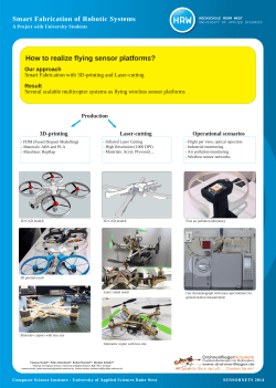
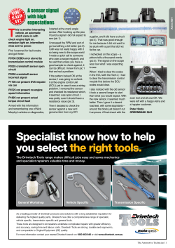


© Copyright 2026