1. sports
2. swimming

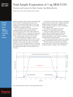
SE-14-001
Methods for Calculation of Evaporation from
Swimming Pools and Other Water Surfaces
Mirza Mohammed Shah, PE, PhD
Fellow/Life Member ASHRAE
ABSTRACT
The calculation of evaporation is required from a variey
of water pools including swimming pools, water storage tanks
and vessels, spent fuel pools in nuclear power plants, etc. The
author has previously published formulas for the calculation
of evaporation from occupied and unoccupied indoor swimming pools, which were shown to agree with all available test
data. In this paper, evaporation from many types of water pools
and vessels is discussed and formulas are provided for calculating evaporation from them. These include indoor and
outdoor swimming pools (occupied and unoccupied), spent
nuclear fuel pools, decorative pools, water tanks, and spills.
Look-up tables are provided for simplifying manual calculations.
INTRODUCTION
This paper attempts to provide reliable methods for the
calculation of evaporation from many types of water pools,
tanks, vessels, and spills. The author has previously published
formulas for the calculation of evaporation from occupied and
unoccupied indoor swimming pools, which were validated
with all available test data (Shah 1992, 2008, 2012a, 2013) and
are widely used. The calculation of evaporation is also
required for many other applications and situations. In this
paper, in addition to the author’s published correlations for
indoor swimming pools, formulas and methods are also
provided for the calculation of evaporation for the following:
•
•
•
•
Outdoor occupied and unoccupied swimming pools
Pools with hot water, such as spent nuclear fuel pools
Decorative pools
Pools used for heat rejection from refrigeration systems
•
•
Vessels/tanks with low water level
Water spills
The calculation methods presented are based on physical
phenomena, theory, and test data.
MECHANISM OF EVAPORATION
Consider evaporation from an undisturbed water surface,
such as that of an unoccupied swimming pool. A very thin
layer of air, which is in contact with water, quickly gets saturated due to molecular movement at the air-water interface. If
there is no air movement at all, further evaporation proceeds
entirely by molecular diffusion, which is a very slow process.
On the other hand, if there is air movement, this thin layer of
saturated air is carried away and is replaced by the comparatively dry room air and evaporation proceeds rapidly.
Thus, it is clear that for any significant amount of evaporation to occur, air movement is essential. Air movement can
occur due to two mechanisms:
1.
2.
Air currents caused by the building ventilation system for
indoor pools and wind for outdoor pools. This is the
forced convection mechanism.
Air currents caused by natural convection (buoyancy
effect). Room air in contact with the water surface gets
saturated and thus becomes lighter compared to the room
air, and therefore moves upwards. The heavier and drier
room air moves downwards to replace it.
For outdoor swimming pools, forced convection is
usually the prevalent mechanism. For indoor pools, natural
convection mechanism usually prevails while most published
formulas have considered only forced convection.
Mirza Mohammed Shah is an independent consultant, Redding, CT.
 2014 ASHRAE. THIS PREPRINT MAY NOT BE DISTRIBUTED IN PAPER OR DIGITAL FORM IN WHOLE OR IN PART. IT IS FOR DISCUSSION PURPOSES ONLY
AT THE 2014 ASHRAE ANNUAL CONFERENCE. The archival version of this paper along with comments and author responses will be published in ASHRAE
Transactions, Volume 120, Part 2. ASHRAE must receive written questions or comments regarding this paper by July 21, 2014 for them to be included in Transactions.
UNOCCUPIED INDOOR SWIMMING POOLS
Present Author’s Method
Shah developed formulas for evaporation from undisturbed water surfaces, which starting with Shah (1981), went
through several modifications (Shah 1990, 1992, 2002, 2008).
The final version is in Shah (2012), according to which the
evaporation rate E0 is the larger of those given by the following
two equations:
E 0 = C w  r – w 
1/3
W w – W r
E 0 = b  pw – pr 
(1)
(2)
with C = 35 in SI units and C = 290 in I-P units, b = 0.00005
in SI and b = 0.0346 in I-P units.
Equation 1 is the evaporation due to natural convection
effect. It was derived using the analogy between heat and mass
transfer. The derivation is given in the Appendix. Equation 2
shows the evaporation caused by the air currents produced by
the building ventilation system. This was obtained by analyzing
the test data for negative density difference as shown in Figure
1. The reasoning was that as natural convection essentially
ceases under such conditions, all the evaporation must be occurring due to forced convection. As noted by the ASHRAE Handbook—HVAC Applications (ASHRAE 2007), air velocities in
typical swimming pools range between 0.05 and 0.15 m/s (10 to
30 fpm). The computational fluid dynamics (CFD) simulations
by Li and Heisenberg (2005) of a large swimming pool showed
very complex airflow patterns along the surface and height of
the pool, but the velocities within 1 m (3 feet) of the water
surface were also in this range. Equation 2 is therefore considered applicable to velocities up to 0.15 m/s (30 fpm).
This method was validated by comparison with test data
from 11 sources in Shah (2012b). Table 1 gives the range of
parameters in each of these data sets. In Shah (2008), the same
database (except the data of Hyldegard [1990]) was also
compared to the ten published correlations listed in Table 2.
Table 3 gives the results of these data analyses. It is seen that
the 113 data points were predicted by the Shah formulas with
a mean absolute deviation of 14.5% giving equal weight to
each data set. All the other correlations gave much inferior
agreement with datal; thus, the Shah method is the most reliable among available methods and therefore may be used for
practical calculations.
For ease of calculation using the Shah method, Equations
1 and 2 and Tables 4 and 5 have been prepared. These tables
give the evaporation rates at discrete values of temperature and
humidity in the range that may occur in swimming pools.
Evaporation at intermediate values can be obtained by linear
interpolation.
2
Figure 1 Analysis of data at negative density difference to
obtain Equation 2 for forced convection evaporation in indoor pools. 1 Pa= 2.953E-4 in. Hg, 1
kg/m2·h = 0.205 lb/ft2·h.
Various Formulas for Undisturbed Water Pools
Many researchers performed tests in which air was blown
or drawn over water surfaces and correlated their own test data
in the form:
E =  a + bu   p w – p r 
(3)
Where a and b are constants and u is the air velocity.
Table 2 lists several such correlations. These are applied to
indoor pools by inserting u  0. Such formulas do not take into
account natural convection, which depends on air density
difference, and hence cannot be expected to be generally
applicable to indoor pools in which natural convection effects
are prevalent. This was pointed out by early researchers. For
example, Himus and Hinchley (1924) performed tests on
evaporation by natural convection as well as with forced
airflow and gave formulas for both cases. They found that
their forced convection formula extrapolated to zero velocity
predicts three times their formula for natural convection.
Lurie and Michailoff (1936) stated that forced convection
equations should not be extrapolated to zero velocity as they
will give erroneous results. Nevertheless, such formulas have
continued to be proposed. The best known among such
formulas is that of Carrier (1918) which is recommended by
ASHRAE (2011) with correction factors called activity
factors.
Many other researchers performed tests under natural
convection conditions and correlated their own data by formulas of the form:
E = a  pw – pr 
n
(4)
SE-14-001
Table 1. Range of Test Data for Undisturbed Water Pools
with which Equations 1 and 2 and Other Formulas were Compared
Pool Area
Researcher
m
2
Hyldegard
(1990)
418
Bohlen
(1972)
ft
2
Water
Temp.
°C
°F
Air Temp.
°C
pw – pr
RH,
%
°F
Evaporation
Rate,
ρr – ρw
3
Pa
in. Hg
kg/m
lb/ft
3
2
Notes
2
kg/m ·h
lb/h·ft
4493 26.1
79.0
28.5 83.3
37
1944
0.574
0.0134
8.4E-4
0.125
0.026
1
32
344
25.0
77.0
27.0 80.6
60
1029
0.303
0.0043
2.7E-4
0.052
0.011
1
Boelter et al.
(1946)
0.073
0.78
24.0 75.2 18.7 65.7
94.2 201.6 24.7 76.5
64
98
1272
80156
0.375
23.7
0.022
1.0025
1.4E-3
0.062
0.082
21.07
0.016
4.2
2
Rohwer
(1931)
0.837
9.0
7.1
16.5
44.5
61.7
6.1 43.0
17.2 63.0
69
78
247
638
0.073
0.188
0.0049
0.0080
3.1E-4
5.0E-4
0.010
0.040
0.0021
0.0082
2
Sharpley and
Boelter (1938)
0.073
0.78
13.9
33.4
57.0
92.1
21.7 71.1
53
210
3786
0.062
1.12
–0.0049
0.088
-3.1E-4
5.5E-3
0.018
0.402
0.0036
0.0804
2
Biasin &
Krumme
(1974)
62.2
668
24.3
30.1
75.7
86.2
24.3 75.7
34.6 94.3
40
68
1010
2128
0.298
0.628
0.0007
0.030
4.4E-5
1.9E-3
0.030
0.154
0.006
0.0301
1
Sprenger (c.
1968)
200
2150 28.5
83.3
31.0 87.8
54
55
1422
1467
0.420
0.433
0.0070
0.0076
4.4E-4
4.7E-4
0.070
0.235
0.014
0.047
1
Tang et al.
(1993)
1.13
12.1
25.0
77.0
20.0 68.0
50
2001
0.591
0.0433
2.7E-3
0.168
0.034
2
Reeker
(1978)
Note 3
23.0
73.4
25.5 77.9
71
493
0.145
–0.004
–2.5E-4
0.0265
0.054.
1, 3
Smith et al.
(1993)
404
4343 28.3
82.9
21.7 71.1
27.8 82.0
51
73
1127
1990
0.332
0.588
0.0150
0.0554
9.4E-4
3.5E-3
0.090
0.246
0.018
0.049
1
Doering
(1979)
425
4568 25.0
77.0
27.5 81.5
28
2142
0.632
0.0153
9.4E-4
0.175
0.035
1
All Sources
0.073
425.0
0.78
7.1 44.5
6.1 43.0
4568 94.2 201.6 34.6 94.3
28
98
210
80156
0.062
23.7
–0.004 –2.5E-4
+1.002 +0.065
0.010
21.073
0.002
4.202
Notes: 1. Field tests on swimming pool 2. Laboratory tests 3. Private pool, size not given
Where a and n are constants. Such formulas do not take into
account density difference, which determines the intensity of
natural convection, and hence cannot be expected to be generally applicable.
Many of the correlations of the type of Equations 3 and 4
are listed in Table 2. As is seen in Table 3, these give poor
agreement with most data.
OCCUPIED INDOOR POOLS
Experience shows that evaporation from occupied pools
is higher than from unoccupied pools. This increase is attributed to an increased area of contact between air and water due
to waves, sprays, wet bodies of occupants, and wetting of
deck. As deck area is usually comparable to the pool area,
wetted deck represents the largest increase in air-water contact
area. The air-water contact area is expected to increase with an
increasing number of occupants. A number of formulas have
SE-14-001
been published according to which the increase in evaporation
compared to unoccupied pools depends only on the number of
occupants (Hens 2009; Smith et al. 1999; Shah 2003). The
basic assumption in these formulas is that the rate of evaporation from the increased air-water contact area is the same as
from the pool area.
Shah (2013) pointed out that the rate of evaporation from
the wetted deck area may not be the same as from the pool
surface. Water spilled on the deck will quickly cool down,
approaching the wet-bulb temperature. If the pool water
temperature is higher than the air temperature, the rate of evaporation from the wetted deck will be much lower than from the
pool surface as the density difference between air and water
will be much lower at the deck, reducing the natural convection intensity. On the other hand, if the water and air temperatures are about equal, the rate of evaporation from the wetted
deck will be comparable to that from the pool surface. Thus,
3
Table 2.
Various Empirical Correlations for Undisturbed Water Pools
Author
Correlation, SI Units
Correlation, IP Units
Carrier (1918)
 0.089 + 0.0782u   p w – p r 
E = -------------------------------------------------------------------i fg
 95 + 0.425u   p w – p r 
E = ---------------------------------------------------------i fg
Smith et al. (1993)
0.76  0.089 + 0.0782u   p w – p r 
E = ------------------------------------------------------------------------------i fg
0.76  95 + 0.425u   p w – p r 
E = --------------------------------------------------------------------i fg
Biasin and Krumme
(1974)
E = – 0.059 + 0.000079  p w – p r 
E = – 0.0118 + 0.0535  p w – p r 
Rohwer (1931)
E = 0.000252  1.8  t w – t r  + 3 
2/3
 pw – pr 
Boelter et al. (1946)
For x < 0.008, E = 5.71 x
For 0.008 < x  0.016,
E = 4.88 (–0.024 + 4.05795 x)
For x > 0.016, E = 38.2 (x)1.25
Boelter et al. (1946)
E = 0.0000162  p w – p r 
Tang et al. (1993)
1.22
E = 0.08  t w – t r + 3 
2/3
 pw – pr 
Forx<5E-4, E=91.4x
For 5E-4 < x  1E-3,
E = 0.98 (–0.024 + 64.92 x)
For x > 1E-3, E = 1222 (x)1.25
E = 0.065  p w – p r 
1.22
E = 0.0000258  p w – p r 
1.2
E = 0.089  p w – p r 
1.2
Leven (c. 1969)
E = 0.0000094  p w – p r 
1.3
E = 0.073  p w – p r 
1.3
E = 0.0000778  p w – p r 
the increase in evaporation due to occupancy depends not only
on the number of occupants but also the density difference
between room air and the air in contact with the pool surface.
Accordingly, Shah presented the following formula for evaporation from occupied pools:
For N*  0.05,
E occ /E 0 = 1.9 – 21   r –  w  + 5.3N *
(5)
where N* is the number of occupants per unit pool area. For
N* < 0.05, perform linear interpolation between Eocc/E0 at
N* = 0.05 persons/m2 (0.0046 persons/ft2) and Eocc/E0 = 1 at
N* = 0. For (r – w) < 0, use (r – w) = 0. E0 is calculated
by the Shah (2012) method, larger of Equations 1 and 2.
In Figure 2, predictions of Equation 5 are plotted together
with the predictions of the correlations of Hens (2009) and
Smith et al. It is seen that at  = 0.05 kg/m3 (0.0031 lb/ft3),
the predictions of Equation 5 and those of Smith et al. (1999)
are almost identical. For  = 0, the predictions of Equation 5
are fairly close to the Hens formula. The formulas of Smith et
al. and Hens were based entirely on their own data. The difference in their predictions is because of the different air and
water conditions in their respective tests. Smith et al. (1993)
report that water temperature was 28.3°C (83°F) and the air
temperature varied from 21.6°C to 27.8°C (71°F to 82.0°F),
with relative humidity from 51% to 73%; these conditions
indicate that  was high. In the tests reported by Hens, air
4
Formula 1
Formula 2
1.237
E = 222(x)
E = 35(x)1.237
Himus and Hinchley
(1924)
Box (1876)
Note
E = 0.054  p w – p r 
temperature was higher than water temperature; these conditions indicate that  was small during the tests.
Equation 5 was compared to test data from four sources
(all that could be found); the range of those data is listed in
Table 6. The data were predicted with a mean absolute deviation of 18%, with deviations of 87% of the data within 30 %.
The same data were also compared with Shah (2003) phenomenological and empirical correlations, ASHRAE Handbook—
HVAC Applications method (2007), and the formulas of Hens
(2009), Smith et al. (1993), and VDI (1994). These correlations are listed in Table 7. The results of the comparison are in
Table 8. While the Shah (2003) correlations performed fairly
well, the others gave poor agreement. Thus Shah (2013),
Equation 5, is easily the most reliable correlation for occupied
pools.
For ease in hand calculations with Equation 5, Tables 9
and 10 list the density differences in the range of air and water
conditions typical for indoor swimming pools. Hand calculations can be done easily using Table 9 or 10 together with Table
4 or 5, depending on the units being used.
Table 11 lists comparison of some individual data points
for occupied and unoccupied indoor swimming pools with
various formulas. It is seen that the Shah (2013) formula gives
much better agreement with the data.
SE-14-001
Table 3.
Results of Comparison of Data for Undisturbed Water Pools from All Sources with All Formulas
Percent Deviation From Correlation of Mean Absolute Average
Number
of Data
Points
Data of
Biasin
and
Box
Krumme
Leven Rohwer
Himus
Boelter
Boelter
Tang
and
et al.,
et al.,
et al.
Hinchley Formula 2 Formula 1
Carrier
Smith
Shah Notes
et al.
Rohwer
(1931)
40
310.3
–310.3
74.6
69.8
40.6
19.9
21.2
6.2
86.2
81.9
44.4
28.4
35.0
–5.3
52.3
42.4
210.5
210.4
137.4
135.9
34.2
12.0
Bohlen
(1972)
1
57.1
–57.1
54.0
54.1
49.9
49.9
NA
104.5
104.5
47.4
47.4
16.7
–16.7
60.5
60.5
181.5
181.5
111.1
111.1
1.0
–1.0
Smith et al.
(1993)
5
56.5
–56.5
20.1
–20.1
9.0
–9.0
30.8
5.4
17.7
17.7
14.3
–14.3
27.6
–27.6
10.1
–10.1
45.3
45.3
9.5
9.5
18.7
–18.7
Boelter
et al. (1946)
24
49.6
–49.6
44.6
–4.3
27.7
27.7
188.9
188.9
31.9
31.4
7.5
0.1
7.3
–3.0
9.9
–4.3
28.2
8.0
30.6
–17.9
12.0
10.2
Sharpley
and Boelter
(1938)
29
59.2
–59.2
39.8
21.1
35.1
31.0
65.9
55.6
72.7
71.9
31.3
24.8
10.1
0.9
38.6
35.3
121.4
121.4
68.4
68.2
16.9
9.0
1
18.7
–18.7
63.0
63.0
76.5
76.5
NA
132.4
132.4
68.7
68.7
34.8
34.8
82.1
82.1
198.0
198.0
126.5
126.5
6.1
6.1
1
9
16.0
–1.0
63.0
63.0
89.7
89.7
40.2
19.6
143.8
143.8
77.9
77.9
67.8
67.8
91.0
91.0
198.0
198.0
126.5
126.5
31.5
31.5
2
Tang et al.
(1993)
1
41.0
–41.0
7.3
–7.3
10.1
10.1
58.6
58.6
40.5
40.5
2.7
2.7
0.0
0.0
9.8
9.8
69.4
69.4
28.7
28.7
7.7
7.7
Reeker
(1978)
1
156.9
–156.9
8.6
8.6
15.3
–15.3
NA
24.4
24.4
11.6
–11.6
39.4
–39.4
1.2
–1.2
98.6
98.5
48.8
48.8
7.0
–7.0
Doering
(1979)
1
37.0
–37.0
4.8
–4.8
15.5
–15.5
NA
40.5
40.5
2.7
2.7
9.9
9.9
9.8
9.8
69.4
69.4
27.0
27.0
21.9
–21.9
Hyldegard
(1990)
1
Note 3
Note 3
Note 3
Note 3
Note 3
Note 3
Note 3
5.0
–5.0
113
137.2
–135.9
52.5
32.8
39.2
30.4
74.4
60.6
73.2
71.4
34.1
24.3
25.8
3.9
40.7
32.8
136.2
132.1
86.8
76.4
22.73
10.2
4
82.7
–82.7
40.6
33.3
39.3
26.5
67.6
67.6
76.6
76.6
34.5
29.3
24.9
2.2
36.5
33.5
121.8
121.8
71.3
67.7
14.5
2.0
5
Biasin and
Krumme
(1974)
Note 3 Note 3 Note 3
All Data
Note: 1. Pool area 200 m2.
Table 4.
Water
Temp.,
°C
2. Pool area 62.2 m2. 3. Not evaluated. 4. Giving equal weight to each data point. 5. Giving equal weight to each data set.
Evaporation from Unoccupied Indoor Swimming Pools by the Shah Formulas in SI Units
Evaporation from Unoccupied Pool (E0), Space Air Temperature, and Relative Humidity
25°C
26°C
27°C
28°C
29°C
30°C
50%
60%
50%
60%
50%
60%
50%
60%
50%
60%
50%
60%
25
0.1085
0.0809
0.0917
0.0636
0.0732
0.0515
0.0639
0.0450
0.0583
0.0382
0.0523
0.0311
26
0.1333
0.1042
0.1171
0.0872
0.0997
0.0693
0.0806
0.0547
0.0679
0.0479
0.0620
0.0408
27
0.1597
0.1289
0.1433
0.1118
0.1262
0.0941
0.1081
0.0753
0.0885
0.0582
0.0723
0.0510
28
0.1877
0.1556
0.1711
0.1380
0.1539
0.1200
0.1360
0.1014
0.1171
0.0818
0.0968
0.0618
29
0.2174
0.1841
0.2006
0.1661
0.1831
0.1477
0.1651
0.1287
0.1463
0.1092
0.1268
0.0888
30
0.2491
0.2146
0.2319
0.1962
0.2142
0.1773
0.1959
0.1579
0.1771
0.1380
0.1575
0.1176
SE-14-001
5
Table 5. Calculated Evaporation Rate from Unoccupied Pools at
Typical Design Conditions by the Shah (2012a) Method in I-P Units
Water
Temp.,
°F
Evaporation from Unoccupied Pool (E0) Space Air Temperature and Relative Humidity
76°F
78°F
80°F
82°F
84°F
86°F
50%
60%
50%
60%
50%
60%
50%
60%
50%
60%
50%
60%
76
0.0213
0.0159
0.0176
0.0120
0.0135
0.0099
0.0123
0.0085
0.0110
0.0069
0.0097
0.0053
78
0.0269
0.0211
0.0232
0.0173
0.0193
0.0133
0.0149
0.0106
0.0132
0.0091
0.0118
0.0075
80
0.0327
0.0266
0.0291
0.0228
0.0252
0.0188
0.0212
0.0146
0.0166
0.0114
0.0141
0.0097
82
0.0390
0.0326
0.0353
0.0287
0.0314
0.0246
0.0274
0.0204
0.0232
0.0160
0.0185
0.0122
84
0.0458
0.0391
0.0420
0.0350
0.0381
0.0309
0.0340
0.0266
0.0298
0.0222
0.0253
0.0176
86
0.0530
0.0461
0.0492
0.0419
0.0452
0.0377
0.0410
0.0333
0.0368
0.0288
0.0323
0.0241
88
0.0608
0.0536
0.0569
0.0494
0.0528
0.0450
0.0486
0.0405
0.0442
0.0358
0.0397
0.0311
90
0.0692
0.0618
0.0651
0.0574
0.0610
0.0529
0.0567
0.0482
0.0522
0.0435
0.0476
0.0386
Pool Occupancy Limits
According to the International Building Code 2006, the
maximum allowable occupancy in swimming pools is 4.6 m2
(50 ft2) of pool surface area per person. This code has been
adapted in many parts of the world. In the U.S., each state and
almost every town has its own code. Some of them have incorporated the International Building Code while some have not
done so. Local authorities should be contacted to find the
applicable regulations.
Recommended Calculation Procedure
The following calculation procedure is recommended:
•
•
For unoccupied swimming pools, calculate evaporation
with Equations 1 and 2 and use the larger of the two.
For occupied swimming pools, calculate E0 as above
and then apply Equation 5.
OUTDOOR SWIMMING POOLS
Unoccupied Pools
Natural convection effects in outdoor pools will be the
same as in indoor pools. The difference will be in the
forced-convection effects. In indoor pools, airflow is due to
building ventilation system, while airflow on outdoor pools
is due to wind. If there were no obstructions such as trees
and buildings, evaporation could be calculated using the
analogy between heat and mass transfer considering the
pool surface to be a heated plate. With this approach, Shah
(1981) derived a simplified equation for evaporation due to
wind velocity, which is given in the Appendix. That equation is applicable if there are no obstructions around the
6
Figure 2 Comparison of the Shah formula (2013) Equation
5 with the correlations of Hens (2009) and Smith
et al. (1999) at two values of air density difference, in lb/ft3, 1 lb/ft3 = 16 kg/m3, 1 ft2 = 0.093 m3.
pool. This is also the case for equations developed from
wind tunnel tests. Most outdoor pools are located close to
buildings and trees which distort the airflow streams.
Hence, formulas developed from tests on actual swimming
pools are preferable. The only one found in the literature is
that by Smith et al. (1999) who measured evaporation from
an unoccupied outdoor swimming pool and fitted the
following equation to their test data:
E 0 =  C 1 + C 2 u   p w – p a /i fg
(6)
SE-14-001
Table 6.
Range of Data for which the Shah (2013) Formula for Occupied Indoor Pools has Been Verified
Source
Pool Area,
m2 (ft2)
Persons,
per m2 (per ft2)
Air Temp.,
°C (°F)
RH,
%
Water Temp.,
°C (°F)
ρr – ρw ,
kg/m3 (lb/ft3)
(pw – pr),
Pa (in. Hg)
Doering (1979)
425
(4575)
0.082 (0.008)
0.167 (0.017)
27.5 (81.5)
29.0 (84.2)
33
41
25.0 (77)
0.0024 (0.00015)
0.0153 (0.00096)
1526 (0.45)
2141 (0.63)
Biasin and
Krumme (1974)
64
(689)
0.016 (0.0015)
0.325 (0.03)
26.0 (78.8)
30.0 (86.0)
46
72
26.0 (78.8)
30.0 (86.0)
–0.0013 (–8 × 10–5)
0.0313 (0.0019)
1067 (0.31)
2087(0.62)
Heimann andRink
(1970)
200
(2153)
0.10 (0.0093)
0.325 (0.039)
31.0 (87.8)
54
55
28.5 (83.3)
0.007 (0.00044)
1422 (0.42)
Hanssen and
Mathisen (1990)
72
(774)
0.028 (0.037)
0.486 (0.045)
30.0 (86.0)
60
65
32.0 (89.6)
0.0312 (0.00195)
0.0421 (0.0026)
2084 (0.62)
2377 (0.70)
All Data
64(689)
425(4575)
0.016 (0.0015)
0.486 (0.045)
26 (78.8)
31 (87.8)
32
72
25 (77)
32 (89.6)
–0.0013 (–8 × 10–5)
0.0421 (0.0026)
1067 (0.37)
2377 (0.7)
Table 7.
Various Correlations for Occupied Pools which Were Evaluated Together with Equation 5
Correlation of
SI Units
I-P Units
ASHRAEHandbook—
HVAC Applications
(2007)
E = 0.000144  p w – p r 
E = 0.1  p w – p r 
Smith et al. (1999)
E = 0.0000106  1.04 + 4.3N *   p w – p r 
E = 0.0072  1.04 + 46.3N *   p w – p r 
VDI (1994)
E = 0.0000204  1 + 8.46N *   p w – p r 
E = 0.014  p w – p r 
Hens (2009)
E = 0.0000409  1 + 8.46N *   p w – p r 
E = 0.028  1 + 91N *   p w – p r 
Shah (2003)
Empirical
E = 0.113 – 0.000079/F U + 0.000059  p w – p r  E = 0.0226 – 0.000016/F U + 0.04  p w – p r 
Shah (2003)
Phenomenological
Table 8.
E/E0 = 3.3FU + 1
E/E0 = 1.3FU + 1.2
E/E0 = 2.5
for FU < 0.1
for 0.1  FU 1
for FU > 1
E/E0 =3.3FU +1 forFU < 0.1
E/E0 = 1.3FU + 1.2 for 0.1  FU  1
E/E0 = 2.5
for FU > 1
Deviations of Various Formulas for Occupied Pools with Test Data
Evaluated Formulas
Data of
ASHRAE
(2007)
VDI
(1994)
Smith
et al. (1999)
Hens
(2009)
Shah (2003)
Empirical
Shah (2003)
Phenom.
Shah (2013)
Equation 5
15.3
60.2
20.6
–42.8
-0.4
–24.3
–7.0
17.2
60.2
21.5
42.8
6.0
29.1
23.9
–34.2
-8.6
–28.6
–51.0
–49.0
–27.0
–18.7
34.2
26.4
28.6
51.0
49.0
27.0
20.1
–4.5
32.7
16.6
–25.4
–8.1
–26.1
–5.5
13.0
32.7
16.6
25.4
14.3
26.1
8.1
39.9
94.3
36.2
–38.8
32.7
–5.1
6.8
44.4
94.3
37.8
38.8
36.2
23.6
17.9
18.3
64.3
20.7
–39.7
8.9
–14.4
–1.1
34.3
69.9
31.0
39.7
30.6
25.3
18.0
Doering (1979)
Hanssen andMathisen (1990)
Heimann and Rink (1970)
Biasin and Krumme (1974)
All data
Note: For each data source, first line is arithmetic average deviation, second line is mean absolute deviation.
SE-14-001
7
Table 9.
Air Density Difference
Density Difference
Water
Temp.,
°C
25°C
ρ r – ρ w at Typical Swimming Pool Conditions in SI Units
ρ r – ρ w , kg/m3 Space Air Temperature and Relative Humidity
26°C
27°C
29°C
30°C
50%
60%
50%
60%
50%
60%
50%
60%
50%
60%
50%
60%
25
0.0185
0.0148
0.0135
0.0096
0.0084
0.0043
0.0034
0
0
0
0
0
26
0.0246
0.0209
0.0196
0.0157
0.0145
0.0104
0.0095
0.0051
0.0044
0
0
0
27
0.0308
0.0271
0.0258
0.0218
0.0207
0.0166
0.0156
0.0113
0.0105
0.0059
0.0054
0.0005
28
0.0370
0.0333
0.0320
0.0281
0.0270
0.0228
0.0219
0.0175
0.0168
0.0122
0.0116
0.0068
29
0.0434
0.0397
0.0384
0.0344
0.0333
0.0292
0.0282
0.0238
0.0231
0.0185
0.0180
0.0131
30
0.0498
0.0461
0.0448
0.0409
0.0397
0.0356
0.0347
0.0303
0.0295
0.0249
0.0244
0.0195
Table 10.
Air Density Difference
Density Difference
Water
Temp.,
°F
76°F
ρ r – ρ w at Typical Pool Conditions in I-P Units
ρ r – ρ w , lb/ft3 Space Air Temperature and Relative Humidity
78°F
80°F
82°F
84°F
86°F
50%
60%
50%
60%
50%
60%
50%
60%
50%
60%
50%
60%
76
0.0011
0.0009
0.0008
0.0005
0.0004
0.0002
0.0001
0
0
0
0
0
78
0.0015
0.0013
0.0012
0.0010
0.0008
0.0006
0.0005
0.0002
0.0001
0
0
0
80
0.0020
0.0017
0.0016
0.0014
0.0013
0.0010
0.0009
0.0006
0.0006
0.0003
0.0002
0
82
0.0024
0.0022
0.0020
0.0018
0.0017
0.0014
0.0013
0.0011
0.0010
0.0007
0.0006
0.0003
84
0.0028
0.0026
0.0025
0.0022
0.0021
0.0019
0.0018
0.0015
0.0014
0.0011
0.0011
0.0008
86
0.0033
0.0031
0.0029
0.0027
0.0026
0.0023
0.0022
0.0020
0.0019
0.0016
0.0015
0.0012
In SI units, C1 = 235, C2 = 206, u is in m/s, p in Pa, ifg in J/kg.
In I-P units C1 = 70.3, C2 = 0.314, u is in fpm, p in in. of Hg,
ifg in Btu/lb.
The wind velocity was measured at 0.3 m (3 ft) above the
water surface and the maximum was 1.3 m/s (264 fpm). There
must have been strong natural convection effects as water
temperature was always higher than the air temperature. Jones
et al. (1994) report that during the companion unoccupied pool
tests in this research program, water temperature was 29°C and
the air temperature varied from 14.4°C to 27.8°C (58°F to
82°F), with relative humidity from 27% to 65% . Thus, the
predictions of this formula at lower velocities do not represent
forced-convection effects. Their measurements at 200 fpm (1
m/s) and higher velocity are likely to be free of natural convection effects. Further, considering that Equation 2 is valid up to
a velocity of 0.15 m/s (30 fpm), the following equation is
proposed for forced-convection effects.
E 0 = a  u/b 
8
28°C
0.7
 pw – pa 
(7)
In SI units, a = 0.00005, b = 0.15 m/s. In I-P units, a = 0.0346,
b = 30 fpm.
This equation is plotted in Figure 3 along with the Smith
et al. correlation Equation 6. Also plotted in this figure is the
following formula given by Meyer (1942) which is among the
most verified for large reservoirs.
E =  a + bu   p w – p a 
(8)
In SI units, a = 0.000116, b = 0.000126, and u in m/s. In I-P
units a = 0.0807, b = 0.000407, and u in fpm.
It is seen that the proposed formulas agrees closely with
with Equation 2 at the velocity of 0.15 m/s (30 fpm) and with
the formulas of Meyer and Smith et al. (1999) at higher velocities. As the Smith et al. (1999) measurements were only upto
a velocity of 1.3 m/s (254 fpm), agreement with the Meyer
formula at higher velocities gives confidence that Equation 7
can be used for a wide range of wind velocities.
SE-14-001
Table 11. Comparison of Some Data Points for
Occupied and Unoccupied Swimming Pools with Various Formulas
Source
Biasin and
Krumme
(1974)
Pool
Area
m2 (ft2)
62.2
(669)
Air
Temp.
°C (°F)
Air
RH,
%
Water
Numberof
Temp.
Persons
°C (°F)
32.2
(90)
51.6
27.9
(82.2)
6
28.0
(82.4)
57.6
30.0
(86.0)
31.0
54.0
31.0
(87.8)
Measured
Evaporation
kg/m2·h
(lb/ft2·h)
Percent Deviation From Formula of
Smith
Hens Shah
et al.
(2009) (2013)
(1993,1999)
ASHRAE
(2011)
VDI
(1994)
0.152
(0.031)
21.0
68.1
28.5
–39.0
0.3
1
0.172
(0.035)
73.2
140.5
43.3
–43.3
14.9
28.5
0
0.07
50.9
6.9
122.0
–14.0
6.0
55.0
28.5
(83.3)
20
0.175
(0.035)
17.0
62.5
27.3
–38.7
–7.3
31.0
(87.8)
55.0
28.5
(83.3)
65
0.235
(0.048)
–12.9
21.0
57.2
–7.3
5.1
Heimann
and Rink
(1970)
200
(2149)
Doering
(1979)
425
(4568)
27.5
(81.5)
34
25
(77.0)
35
0.212
(0.043)
30.5
81.3
34.6
–37.2
12.9
Hansen
and
Mathieson
(1990)
72
(774)
30.0
(86.0)
63
32
(89.6)
27
0.60
(0.122)
–50.0
–30.5
–1.8
–40.8
–9.7
Hyldgaard
(1990)
418
(4493)
28.5
(83.3)
37.0
26.1
(79.0)
0
0.125
(0.026)
12.0
–20.7
64.7
–36.4
–5.0
Bohlen
(1972)
32 (344)
27.0
(80.6)
60.0
25.0
(77.0)
0
0.052
(0.011)
42.3
0.9
110.8
–19.1
–1.0
Reeker
(1978)
Not
Given
25.5
(77.9)
71.0
23.0
(73.4)
0
0.026
(0.0054)
33.9
-5.1
95.7
–23.0
–7.0
Effect of Occupancy
Smith et al. (1999) report results of their tests on both
indoor and outdoor swimming pools, occupied and unoccupied. They found no difference in the effect of occupancy on
evaporation rate between indoor and outdoor pools. This is
what would be expected from the physical phenomena
involved. Hence, Equation 5 is also applicable to outdoor
pools.
Effect of Solar Radiation and Radiation to Sky
Solar radiation adds heat to pool water and thus reduces
the energy needed for heating the pool. Further, the pool loses
heat by radiation to the sky, which has to be made up by additional heating. These heat gains and losses have to be taken into
consideration in the calculation of pool energy requirements.
As seen in the formulas above, the rate of evaporation depends
only on the water temperature and air conditions. In heated
pools, water temperature is maintained constant by the heating
system, and, hence, loss or gain by radiation is not involved in
the calculation of evaporation. For unheated pools, water
temperature has to be calculated taking into consideration all
SE-14-001
heat gains and losses, including those by radiation. The calculation of evaporation is then done using the calculated water
temperature.
Recommended Calculation Procedure
for Outdoor Pools
The following calculation procedure is recommended for
outdoor swimming pools:
•
•
For unoccupied pools, calculate evaporation by Equations 1, 2, and 7. Use the largest of the three.
For occupied pools, calculate E0 as above and then
apply Equation 5.
POOLS CONTAINING HOT WATER
A notable example of pools with hot water is the pool for
storing spent fuel in nuclear power plants. During normal
operation, water temperature could be up to 50°C (122°F). If
cooling for the pool is lost during an abnormal/accidental
event, temperatures can rise to boiling point. The Shah
formula for natural convection has been verified for water
temperatures up to 94°C (201°F) Shah (2002). Figure 4 shows
9
Figure 3 Comparison of the proposed new formula for
evaporation, Equation 7, due to forced airflow,
with the formulas of Smith et al. (1999) and Meyer
(1944), 1 kg/m2·h = 0.205 lb/ft2·h, 1 m/s = 0.3048
ft/s.
the comparison of the data of Boelter et al. (1946) with the
Shah formula. Air temperature during these tests varied from
19°C to 25°C (66.2°F to 77.0°F) and the relative humidity
from 64% to 98 %. The agreement is excellent throughout the
range of water temperature.
Hugo (2013) provided the author with preliminary data
from the fuel pool of a nuclear power plant (Columbia Generating Station). The pool dimensions were 10.4 × 22.6 m (34 ×
40 ft). He measured the increase in evaporation as water
temperature rose above 36.7°C (98°F). Air temperature was
25.5°C (78°F) and its relative humidity was 57 %. Air velocity
above the pool was 0.31 m/s (62 fpm). To get the total evaporation, evaporation at 36.7°C (98°F) was calculated by the
Shah method described in the foregoing (largest of the values)
and added to the measurements at other water temperatures.
These were then compared with the Shah correlation as the
larger of the free and forced convection evaporation, as calculated with Equation 1 and 7. The comparison of measured and
predicted evaporation is shown in Figure 5. Good agreement
is seen. Considering the good agreement with high temperature data of Boelter et al. (1946) and Hugo (2013), the Shah
method can be confidently used for high-temperature pools.
For ease in hand calculations, Tables 12 and 13 have been
prepared in SI and I-P units respectively. These list evaporation rates at discrete values of temperature and relative humidity, calculated as the larger of those from Equations 1 and 2.
Calculations for intermediate values can be done by linear
interpolation. Do not use these tables if air velocity is higher
than 0.15 m/s (30 fpm).
10
Figure 4 Comparison of the data of Boelter et al. (1946)
with the predictions of the Shah correlation
(2012a), Equations 1 and 2, 1 kg/m2·h = 0.205 lb/
ft2·h.
Figure 5 Comparison of data of Hugo (2013) for evaporation from a nuclear fuel pool with the Shah
formula. Building air temperature 25.5°C (78°F),
relative humidity 57%, 1 kg/m2·h = 0.205 lb/ft2·h.
Recommended Calculation Procedure
The following procedure is recommended for calculation
of evaporation from pools containing hot water:
•
Calculation procedure is the same as for unoccupied
swimming pools: calculate evaporation by Equations 1,
2, and 7 and use the largest of the three.
•
Calculations may alternatively be done with Table 12 or
13 if air velocity does not exceed 0.15 m/s (30 fpm).
SE-14-001
Table 12. Calculated Evaporation Rates at High Water Temperatures
by the Shah Correlation (2012a), Larger of Equations 1 and 2, SI Units
Air Temperature, °C, and Relative Humidity, %
Water
Temp., oC
30°C
35°C
40°C
45°C
50°C
30°C
70°C
30°C
70°C
30°C
70°C
30°C
70°C
30°C
70°C
35
0.443
0.246
0.350
0.116
0.236
0.023
0.138
0
0.096
0
40
0.707
0.485
0.608
0.332
0.495
0.165
0.033
0.033
0.184
0
45
1.057
0.816
0.951
0.644
0.830
0.448
0.691
0.232
0.530
0.047
50
1.516
1.26
1.403
1.072
1.274
0.853
1.126
0.603
0.956
0.325
55
2.113
1.845
1.992
1.643
1.855
1.405
1.698
1.128
1.517
0.809
60
2.879
2.603
2.752
2.390
2.607
2.137
2.441
1.839
2.251
1.489
65
3.856
3.576
3.721
3.352
3.569
3.088
3.396
2.775
3.198
2.403
70
5.088
4.809
4.948
4.578
4.790
4.306
4.661
3.983
4.407
3.598
75
6.632
6.358
6.486
6.123
6.323
5.847
6.140
5.520
5.932
5.130
80
8.550
8.288
8.400
8.053
8.234
7.778
8.049
7.453
7.840
7.066
85
10.92
10.67
10.76
10.44
10.60
10.17
10.41
9.859
10.21
9.487
90
13.81
13.60
13.66
13.38
13.49
13.12
13.31
12.83
13.12
12.48
Table 13. Calculated Evaporation Rates at High Water Temperatures
by the Shah Correlation (2012a), Larger of Equations 1 and 2, I-P Units
Air Temperature, °F, and Relative Humidity, %
Water
Temp., °F
90°F
100°F
110°F
120°F
30°F
70°F
30°F
70°F
30°F
70°F
30°F
70°F
100
0.111
0.063
0.087
0.029
0.058
0.004
0.031
0
110
0.182
0.128
0.157
0.088
0.27
0.043
0.092
0.006
120
0.278
0.220
0.251
0.175
0.22
0.122
0.183
0.062
130
0.408
0.346
0.379
0.297
0.345
0.238
0.306
0.168
140
0.58
0.516
0.549
0.463
0.513
0.399
0.471
0.323
150
0.805
0.740
0.772
0.684
0.735
0.617
0.691
0.536
160
1.097
1.032
1.063
0.975
1.023
0.905
0.978
0.821
170
1.471
1.408
1.435
1.35
1.395
1.28
1.349
1.195
180
1.946
1.887
1.91
1.829
1.869
1.760
1.823
1.677
190
2.544
2.491
2.507
2.435
2.467
2.37
2.423
2.291
200
3.290
3.246
3.254
3.194
3.215
3.134
3.173
3.064
SE-14-001
11
VARIOUS POOLS AND TANKS
For pools in residences, condominiums, hotels, and therapeutic pools, the methods for indoor and outdoor swimming
pools presented earlier in this paper are recommended. The
ASHRAE Handbook—HVAC Applications (2007, 2011)
recommends activity factors which give lower evaporation
rates from such pools compared to public pools. The
ASHRAE activity factors are based on experience and probably indicate that these pools have lower occupancy compared
to public pools. While calculating evaporation with the present
method, occupancy based on experience should be used.
Water pools are often provided inside and outside buildings to enhance aesthetics. In hot, dry climates, water pools
provide evaporative cooling in naturally ventilated buildings.
Outdoor pools are often used to provide cooling water for the
condensers of refrigeration plants. Evaporation in all such
pools can be calculated by the methods presented earlier for
unoccupied indoor and outdoor swimming pools.
The same methods are recommended for various tanks
and vessels containing water.
EFFECT OF EDGE HEIGHT OR LOW WATER LEVEL
If the water level is lower than the top edge of the pool or
vessel, one will expect some impairment of natural convection
currents and hence some reduction in evaporation. This effect
will be expected to increase with increasing (/d) where  is
the edge height and  is the equivalent diameter of the vessel
or pool. This possible effect has been investigated by several
researchers.
Sharpley and Boelter (1938) measured evaporation into
quiet air from a 0.305 m (1 ft) diameter pan. The water level
was flush with top. Tests were also performed with water level
12.7 and 38.1 mm (0.5 and 1.5 in.) below the top edge. Thus,
(/d) varied from 0 to 0.125. Sharpley and Boelter found no
effect of liquid level variation. Hickox (1944) also did similar
tests. His data do not show any clear effect of level variation.
Stefan (1884) measured evaporation from tubes of diameter 0.64 to 6.16 mm (0.025 to 0.24 in.) and depth below the
rim of 0 to 44 mm (0 to 1.7 in.). He found the evaporation rate
to be inversely proportional to the depth. Considering the
larger tube, (/d) at 44 mm (17.3 in.) depth below the top
would be 7.1. As noted earlier, reduction in evaporation at
large (/d) is expected as inward and outwards movement of
natural convection streams of air will be hampered. At very
large depths, evaporation will be entirely due to molecular
diffusion.
For large values of (/d), evaporation by forced convection will also be impaired as airstream will be unable to
remove the air layers near the water surface.
In swimming pools, the water level is close to the top and
hence there is no reduction in evaporation. For other types of
pools and vessels in which water level is very low, the predictions by the Shah method will need to be corrected. Details of
Stefan’s tests are not available and no other test data were
12
found. Based on the results of Stefan (1884) mentioned earlier,
the following is tentatively suggested as a rough guide:
For  /d  1 ,
E = E shah  /d 
is  E md
(9)
Where Eshah is the evaporation rate by the Shah method and
Emd is the evaporation by molecular diffusion. Methods to
calculate evaporation by molecular diffusion are explained in
text books as well as in Chapter 6 of the ASHRAE Handbook—Fundamentals (2013).
EVAPORATION FROM WATER SPILLS
Water spilled on the floor will cool down fairly quickly,
approaching the wet-bulb temperature of air. If it reaches the
wet bulb temperature, the difference of density between room
air and the air at water surface will be zero, there will be no
natural convection, and evaporation will be due to forced
convection. Hence, the following simple method is suggested
for approximately calculating evaporation rate from spills:
1.
Assume water temperature to be equal to the wet-bulb
temperature of air.
2.
For spills inside buildings, use Equation 2 to calculate
evaporation.
3.
For outdoor spills, use Equation 7 to calculate evaporation.
More rigorous transient calculations may be done with a
computer model that takes into consideration heat transfer
between the floor and water together with heat and mass transfer between air and water. The Shah correlation may be incorporated into such a model.
SUMMARY OF
RECOMMENDED CALCULATION METHODS
The calculation methods recommended in the foregoing
are summarized in Table 14.
CONCLUSION
In this paper, methods for calculating evaporation from
many types of pools and other water surfaces were presented
and discussed. These include the author’s published correlations for indoor occupied and unoccupied swimming pools.
Also presented were methods for outdoor occupied and unoccupied swimming pools, hot-water pools such as nuclear fuel
pools, decorative pools, tanks and vessels/containers, and
water spills. These methods are based on theory, physical
phenomena, and test data. A number of look-up tables were
provided for easy manual calculations.
More tests to collect data on evaporation from swimming
pools is highly desirable, especially for occupied pools as data
from only four sources could be found.
SE-14-001
Table 14.
Application
Summary of Recommended Calculation Methods
Calculation Method
Notes
Indoor swimming pool, unoccupied
Use larger of Equations 1 and 2
Tables 4 and 5 may be used for manual calculations
Indoor swimming pool, occupied
Use Equation 5
Tables 9 and 10 may be used with Tables 4 and 5 for
manual calculations
Outdoor swimming pool, unoccupied
Use largest of Equations 1, 2, and 7
Outdoor swimming pool, occupied
Use Equation 5
—
E0 by the method for outdoor unoccupied pools
Various types of pools, indoor or outdoor Same as for unoccupied swimming pools
For indoor hot-water pools, Tables 12 and 13 may
be used for manual calculations
Vessels, tanks, containers
Same as for unoccupied swimming pools
If water level is very low, correct prediction with
Equation 9
Water spills
Assume water is at wet-bulb temperature
For more accuracy, perform computerized transient
of air and then calculate as for unoccupied
calculations considering all factors
swimming pool
ACKNOWLEDGEMENT
The author thanks Mr. Bruce Hugo for providing the data
from his ongoing tests on evaporation from a nuclear fuel pool.
Thanks are also due to Mr. Rui Igreja for checking the lookup tables in the author’s previous publications and pointing out
some discrepancies.
NOMENCLATURE
A
d
D
E
Eocc
E0
FU
g
Gr
ifg
hM
L
N
N*
Nu
p
Pr
ReL
Sc
= area of water surface, m2 (ft2)
= diameter or equivalent diameter of vessel/tank, m
(ft). Equivalent diameter = (A/0.785)0.5
= coefficient of molecular diffusivity, m2/h (ft2/h)
= rate of evaporation under actual conditions, kg/m2·h
(lb/ft2·h)
= rate of evaporation from occupied swimming pool,
kg/m2·h (lb/ft2·h)
= rate of evaporation from unoccupied pools, kg/m2·h
(lb/ft2·h)
= pool utilization factor, = 4.5 N* (42N*), dimensionless
= acceleration due to gravity, m/s2 (ft/s2)
= Grashof number, dimensionless
= latent heat of vaporization of water, J/kg (Btu/lb)
= mass transfer coefficient, m/h (ft/h)
= characteristic length m (ft)
= number of pool occupants
= N/A, persons/m2 (persons/ft2)
= Nusselt number, dimensionless
= partial pressure of water vapor in air, Pa (in. Hg)
= Prandtl number, dimensionless
= Reynolds number = uL/µ, dimensionless
= Schmidt number = /D, dimensionless
SE-14-001
Sh
u
W
x
x
= Sherwood number, = hML/D, dimensionless
= air velocity, m/s (fpm)
= specific humidity of air, kg of moisture/kg of air (lb
of moisture/lb of air)
= concentation of moisture in air, kg of water/m3 of air
(lb of moisture/ft3 of air)
= (xw – xr), kg/m3 (lb/ft3)
Greek Symbols




= depth of water level below top edge, m (ft)
= dynamic viscosity of air, kg/m·h (lb/ft·h)
= density of air, mass of dry air per unit volume of
moist air, kg/m3 (lb/ft3) (This is the density in
psychrometric charts and tables)
= (r – w), kg/m3 (lb/ft3)
Subscripts
a
H
M
r
w
=
=
=
=
=
of air away from the water surface
heat transfer
mass transfer
at room temperature and humidity
saturated at water surface temperature
APPENDIX
Derivation of Formula for Evaporation by
Natural Convection
The formula is derived using the analogy between heat
and mass transfer, considering the water surface to be a horizontal plate with the heated face upwards.
The rate of evaporation is given by the relation (Eckert
and Drake 1972)
13
E 0 = h M w  W w – W r 
(A1)
The air density  has been evaluated at the water surface
temperature as recommended by Kusuda (1965).
Heat transfer during turbulent natural convection to a
heated plate facing upwards is given by the following relation
(McAdams 1954):
Nu = 0.14  Gr H Pr 
1/3
(A2)
Using the analogy between heat and mass transfer, the
corresponding mass transfer relation is
Sh = 0.14  Gr M Sc 
1/3
(A3)
3 2
g  W w – W r L 
Gr M = ---------------------------------------------2

(A4)
where
1 
 = – ---  ---------
  W 
(A5)
r – w
 = ------------------------------W w – W r 
(A6)
Combining Equations A4 and A6
3
(A7)
Using Equation A7 and the definitions of Sh and Sc,
Equation A3 becomes
(A8)
Combining Equations A1 and A8:

w  r – w 
1/3
W w – W r
(A9)
The value of (D2/3 –1/3) does not vary much over the typical range of room air conditions. Inserting a mean value, Equation A9 becomes:
E 0 = C w  r – w 
1/3
W w – W r
(A10)
with C = 35 in SI units and 290 in I-P units.
It is noteworthy that Equations A9 and A10 have been
derived from theory without any empirical adjustments. Equa14
1/3
(A11)
Using the analogy between heat and mass transfer, the
corresponding mass transfer relation is
1/3
(A12)
The viscosity and Schmidt number of air change very
little over the typical air conditions. Taking a mean value for
them and substituting an empirical relation for the coefficient
of diffusivity, the following formula is obtained for air-water
in SI units.
E 0 =  0.0016t + 0.22 L
0.8
–1
(A13)
– 256  w  W w – W a 
Where u is the free stream velocity in m/min and L is the
length of pool in the direction of air in meters.
In I-P units, the equation is:
 3.5  Lu a 
0.8
–1
(A14)
– 256  w  W w – W a 
Where u is in fpm and L is in feet..
The above derivation is from Shah (1981).
REFERENCES
3 1/3
hM L
  r –  w g L
---------- = 0.14 -------------------------------D
D
2/3 – 1/3
Nu =  0.036 Re L – 836 Pr
E 0 =  0.0092t + 2.07 L
g   r –  w L 
Gr M = -----------------------------------2

D
For heat transfer during flow of air over a heated horizontal plate with turbulent flow, the mean Nusselt number for the
plate is given by
 2.54  Lu a 
Equation A5 may be approximately written as
1/3
Derivation of Formulas for Evaporation by
Forced Convection
Sh =  0.036 Re L – 836 Sc
GrM is defined as (Eckert and Drake 1972)
E 0 = 0.14g
tion A10 was first published in Shah (1992); the detailed derivation was published in Shah (2008).
ASHRAE. 2007. ASHRAE Handbook—HVAC Applications.
Atlanta: ASHRAE.
ASHRAE. 2011. ASHRAE Handbook—HVAC Applications.
Atlanta: ASHRAE.
ASHRAE 2013. ASHRAE Handbook—Fundamentals.
Atlanta: ASHRAE.
Biasin, K., and W. Krumme. 1974. Die wasserverdunstung
in einem innenschwimmbad. Electrowaerme International 32(A3):A115—A129.
Boelter, L.M.K., H.S. Gordon, and J.R. Griffin. 1946. Free
evaporation into air of water from a free horizontal quiet
surface. Industrial & Engineering Chemistry 38(6):596–
600.
Bohlen, W.V. 1972. Waermewirtschaft in privaten, geschlossenen Schwimmbaedern–Uberlegungen zur Auslegung
und Betriebserfahrungen, Electrowaerme International
30(A3):A139–A142.
SE-14-001
Box, T. 1876. A Practical Treatise on Heat. Quoted in Boelter et al. (1946).
Carrier, W.H. 1918. The Temperature of evaporation
ASHVE Trans., 24: 25–50.
Doering, E. 1979. Zur auslegung von luftungsanlagen fur
hallenschwimmbaeder. HLH 30(6):211–16.
Eckert, E.R.G., and R.M. Drake. 1972. Analysis of Heat and
Mass Transfer. New York: McGraw-Hill.
Hanssen, S.A.,and Mathisen, H.M. 1990 Evaporation from
swimming pools. Roomvent 90:2nd International Conference, Oslo, Norway.
Heimann and Rink. 1970. Quoted in Biasin & Krumme
(1974)
Hens, H. 2009. Indoor climate and building envelope performance in indoor swimming pools. Energy efficiency and
new approaches, Ed. by N. Bayazit, G. Manioglu, G.
Oral, and Z. Yilmaz., Istanbul Technical University:
543–52.
Hickox, G.H. 1944. Evaporation from a free water surface.
Proceedings ASCE 70: 1297–327.
Himus, G.W., and J.W. Hinchley. 1924. The effect of a current of air on the rate of evaporation of water below the
boiling point. Chemistry and Industry. August(22):
840–45.
Hugo, B. R. 2013. Personal communication. Seior Reactor
Opeartor at the Columbia Generating Station and
researcher at Washington State University. Email.
Hyldgaard, C.E. 1990. Water evaporation in swimming
baths.: Roomvent 90, International Conference on Engineering Aero- and Thermodynamics of Ventilated
Rooms, Oslo, Norway.
Jones, R., C. Smith, and G. Lof. 1994. Measurement and
analysis of evaporation from an inactive outdoor swimming pool. Solar Energy 53(1):3
Kusuda, T. 1965. Calculation of thE Temperature Of A Flat
Platewet Surface Under Adiabatic Conditions With
Respect To The Lewis Relation. Humidity and Moisture,
vol. 1, edited by R. E. Ruskin, Rheinhold: 16–32.
Leven, K. Betrag zur Frage der wasserverdunstung. Warme
und Kaltetechnik 44(11):161–67.
Li, Z., and P. Heisenberg. 2005. CFD simulations for water
evaporation and airflow movement in swimming baths.
Report, Dept. of Building Technology, University of Aalborg: Denmark.
Lurie, M., and N. Michailoff. 1936. Evaporation from free
water surfaces. Industrial and Engineering Chemistry
28(3):345–49.
McAdams, W.H. 1954. Heat Transmission. New York:
McGraw Hill.
SE-14-001
Meyer, A.F. 1942. Evaporation from Lakes and Reservoirs.
Minnesota Resources Commission.
Rohwer, C. 1931. Evaporation from free water surfaces. Bulletin No. 271. United States Department of Agriculture.
Reeker, J. 1978. Wasserverdunstung in hallenbaedern.
Klima + Kaelte-Ingenieur 84(1):29–33.
Shah, M.M. 1981. Estimation of Evaporation from Horizontal Surfaces. ASHRAE Trans., 87(1)35–51.
Shah, M. M. 1990. Calculating evaporation from swimming
pools. Heating/Piping/Air Conditioning December:
103–105.
Shah, M.M. 1992. Calculation of evaporation from pools
and tanks. Heating/Piping/Air Conditioning April:
69–71.
Shah, M.M. 2002. Rate of evaporation from undisturbed
water pools: Evaluation of available correlations. International J. HVAC&R Research 8(1):125–32.
Shah, M.M. 2003. Prediction of evaporation from occupied
indoor swimming pools.
Energy & Buildings,
35(7):707–13.
Shah, M.M. 2008. Analytical formulas for calculating water
evaporation from pools. ASHRAE Transactions.
114(2)610–18:
Shah, M.M. 2012a. Calculation of evaporation from indoor
swimming pools: further development of formulas.
ASHRAE Transactions 118(2):460–66:
Shah, M.M. 2012b. Improved method for calculating evaporation from indoor water pools. Energy & Buildings.
49(6):306–09.
Shah, M.M. 2013. New correlation for prediction of evaporation from occupied swimming pools. ASHRAE Transactions 119(2)450–55:
Sharpley, B.F., and L.M.K. Boelter. 1938. Evaporation of
water into quiet air from a one-foot diameter surface.
Industrial & Engineering Chemistry 30(10):1125–31.
Smith, C.C., R. Jones, and G. Lof. 1993. Energy requirements and potential savings for heated indoor swimming
pools. ASHRAE Transactions 99(2):864–74.
Smith, C.C., G.O.G. Lof, and R. W. Jones. 1999. Rates of
evaporation from swimming pools in active use.
ASHRAE Transactions 104(1):514–23.
Sprenger, E. 1968. Verdunstung von wasser aus offenen
oberflaechen. Heizung und Luftung 17(1):7–8.
Stefan. 1884. Sitzber. K. K. Akad. Wien. 68: 385-423.
Tang, T.D., M.T. Pauken, S.M. Jeter, and S.I. Abdel-Khalik,
1993. On the use of monolayers to reduce evaporation
from stationary water pools. Journal of Heat Transfer
115(1993):209–14.
VDI. 1994. Wärme, Raumlufttechnik, Wasserer- und –entsorgung in Hallen und Freibädern. VDI 2089.
15