1. family and parenting
2. children

Thyroid Cancer Following Scalp Irradiation:
A Reanalysis Accounting for Uncertainty in
Dosimetry
July 18, 2000
Daniel W. Schafer, Jay H. Lubin, Elaine Ron, Marilyn Stovall and
Raymond J. Carroll
Abstract
In the 1940's and 1950's, children in Israel were treated for tinea capitis (ringworm)
by irradiation. Follow{up studies showed that the radiation was associated with the development of malignant thyroid neoplasms. Despite this clear evidence of an eect, the
magnitude of the dose{response is much less clear because of errors in dosimetry. These
errors have the potential to bias dose{response estimation, a potential that was not
widely appreciated at the time of the original analyses. We revisit this issue, describing
in detail how errors in dosimetry might occur, and we develop a new dose{response
model that takes the uncertainties of the dosimetry into account. Our model for the
uncertainty in dosimetry is a complex and new variant of the classical multiplicative
Berkson error model, having components of classical multiplicative measurement error
as well as missing data. Analysis of the tinea capitis data suggest that measurement
error in the dosimetry has only a negligible eect on dose{response estimation and
inference.
Berkson measurement error; Dose uncertainty; Likelihood; Measurement
error; Missing data; Person{year tables; Poisson regression; Regression calibration; Structural models; Survival analysis.
Accounting for Uncertainty in Radiation Dosimetry
KEY WORDS:
Short title:
AUTHOR AFFILIATIONS AND
ACKNOWLEDGMENTS
Daniel W. Schafer ([email protected]) is Professor, Department of Statistics, 44 Kidder
Hall, Oregon State University, Corvallis, OR 97331-4606.
Jay H. Lubin ([email protected]) is Mathematical Statistician, Biostatistics Branch,
and Elaine Ron ([email protected]) is Chief, Radiation Epidemiology Branch, both
with the Division of Cancer Epidemiology and Genetics, National Cancer Institute, Executive
Plaza North, Room 431, 6130 Executive Boulevard, MSC 7368, Bethesda MD 20892{7368.
Marilyn Stovall ([email protected]) is Associate Professor, Department of Radiation Physics, University of Texas M. D. Anderson Cancer Center, 1515 Holcombe Boulevard, Houston TX 77030.
Raymond J. Carroll ([email protected]) is Distinguished Professor, and Professor in the
Department of Statistics, the Department of Epidemiology and Biostatistics, the Faculty
of Nutrition and the Faculty of Toxicology, Texas A&M University, TAMU 3143, College
Station, TX 77843-3143.
Carroll's research was supported by a grant from the National Cancer Institute (CA57030),
through the Texas A&M Center for Environment and Rural Health via a grant from the National Institute of Environmental Health Sciences (P30-ES09106). Carroll's research partially
occurred during a visit to the Centre for Mathematics and its Applications at the Australian
National University, with partial support from ARC Large Research Grant A00000506.
1 INTRODUCTION
In the 1940's and 1950's, approximately 11,000 children in Israel received radiation therapy
for tinea capitis (ringworm). The purpose of the treatments was to deliver a reasonably
uniform dose of approximately 7 Gy to the scalp in order to produce epilation (Adamson,
1909; Schulz & Albert, 1968). The radiation therapy consisted of ve elds to the scalp
(anterior, posterior, right and left laterals, and vertical), with lead shielding over the face
and neck. The patients wore a cap that positioned the elds, but they were not immobilized during treatment. The beams were supercial x{rays, 70{100 kVp, half{value layer of
approximately 1.0 mm A1.
Several investigators have assessed the late eects of radiation therapy, including the
incidence of thyroid tumors (Modan, et al., 1977; Ron, et al., 1989; Ron, et al., 1995). The
thyroid gland is highly sensitive to the carcinogenic eects of ionizing radiation. Ron, et al.
(1989) note that the Israel study \is one of the few human studies reporting a signicant
risk of cancers at doses on the order of 10 cGy".
The study is described more fully in Section 2, but the major issue for this paper involves the dosimetry in converting a recorded course of radiation therapy into a dose to the
thyroid. In their analysis of the tinea capitis data, Ron, et al. (1989) used the results of
anthropomorphic phantom studies (Modan, et al., 1977; Lee & Youmans, 1970; Schulz &
Albert, 1968) to construct a dose to the thyroid from the child's age at rst irradiation,
ltration of the x{ray machine. prescribed radiation exposure in Roentgens and number of
treatments.
At the time of the analysis reported by Ron, et al. (1989), the potential biases due to
dose imprecision in relative risk regression were not as widely appreciated as they are today.
More recent articles (Pepe, Self & Prentice, 1989; Pierce, Stram & Vaeth, 1990; Pierce,
Stram, Vaeth & Schafer, 1992; Nakamura, 1992; Hughes, 1993; Thomas, Stram & Dwyer,
1993; Lubin, Boice & Samet, 1995; Hu, Tsiatis & Davidian, 1998) have heightened the
awareness of the problem and have provided solutions in various situations. The workshop
1
(Ron
& Homan, 1999) was particularly inuential in motivating a reexamination of the tinea
capitis data.
The purpose of this paper is to reconsider the tinea capitis study to see whether the
thyroid radiation dose uncertainties have an eect on the reported dose{response relationship and on the modifying eects of age at exposure. We will also provide a reanalysis that
accounts for uncertainties. A major component of this work is the formal incorporation of
"external prediction data" into the analysis. By this we mean something like the standard
idea of "external validation data" (Carroll, Ruppert & Stefanski, 1995, Chapter 1) in which
dose and estimated dose are available on an external data set, the dierence in the tinea capitis data being that instead we observe only estimated dose and predictor variables for dose.
The use of an externally estimated prediction equation leads to a multiplicative Berkson{
type model, but with a classical measurement error component due to the estimation of
parameters in the prediction equation. Two additional diÆculties complicate the analysis:
the dose predictor variables are missing for many patients and the use of the external data
set, which is based on phantoms (simulated human bodies exposed in the same way as actual
patients), misses some of the sources of dose uncertainty in live humans. Some speculation
is necessarily required therefore, and sensitivity analysis is used to study the ramications
of this speculation.
The outline of the paper is as follows. In Section 2, we describe the data set in some
detail. Section 3 provides details of the dosimetry modeling. Section 4 describes likelihood
analyses. Section 5 gives our reanalysis of the data. Section 6 gives concluding remarks.
Technical details are given in an appendix.
Uncertainties in Radiation Dosimetry and Their Impact on Dose{Response Analysis
2 DESCRIPTION OF THE DATA SET
The study population consists of 10; 834 persons who received x{ray therapy between 1948{
1960, 10; 834 nonirradiated population matched controls and 5; 392 nonirradiated tinea{free
2
siblings. All the irradiated subjects were less than 16 years old at treatment. Study subjects either immigrated to Israel from Africa or Asia or were children of fathers who had
immigrated from the same regions. Thyroid cancers occurring between 1960{1986 were ascertained by computer linkage of the study subject roster with the Israel Cancer Registry and
were subsequently validated individually. Among the irradiated subjects, 43 developed malignant thyroid tumors and 55 developed benign tumors. Among the nonirradiated subjects,
16 developed malignant thyroid tumors and 41 developed benign tumors.
We decided for simplicity to ignore both kinds of matching and treat subjects as if their
responses are independent. We are justied in doing this for the nonexposed matched controls
since we include the matching variables (age, sex, country of origin) as explanatory variables
in the regression model. We are not justied in treating the siblings as independent, but
since there are only 6 of these siblings who developed thyroid cancer, none of whom had
a treated sibling who developed thyroid cancer, it is unlikely that correctly accounting for
sibling dependence, which would greatly complicate the analysis, will make any dierence. It
should be noted that there is a potential non{independence from members of the same family
being included in the set of exposed patients. The familial connections were not recorded,
however, so we must proceed under the assumption that any eect of familial dependence
must be small relative to the nal resolution of dose-response here. The same assumption
was made by Ron, et al. (1989) and Ron, et al. (1995).
Table 1 summarizes the number of thyroid cancers observed by 1986. Some subjects were
irradiated for ringworm more than once, as indicated in the column \Number of Courses".
Of interest in this paper is inference about parameters in a relative risk regression model.
Particular attention is given to models of the following form for the age{specic thyroid
cancer rate (hazard function) as a function of total radiation dose to the thyroid, D, and
additional covariates X :
h(tjX; D; B) = expfX T (t)
br
In (1), X = X (t) = (X
br
;X
em
br
h
i
g 1 + D expf + X T (t) g :
dr
em
em
(1)
), where X is a vector of those covariates associated with
br
3
Number of Database
Number of Number of cancers
average
courses
subjects per 1000
dose
0
16226
1.0
0.0
1
9814
4.0
8.4
2
904
5.5
17.5
3
110
0.0
25.7
4
6
0.0
27.0
Table 1: Basic statistics for the tinea capitis data base, and the results of the dosimetry.
Here \Database average dose" is the average dose (in centi{Grays) as listed in the data base.
background rate (hence \br"), such as time since rst exposure, while X is a vector of those
covariates that modify the radiation dose{response, i.e., eect modiers (hence \em"). In
what follows, we will suppress the dependence of X on t. The parameters B = ( ; ; )
are associated with (X ; X ; D), and hence control background rate, eect modiers and
dose response (hence \dr"), respectively.
Standard techniques (Breslow, Lubin, Marek, & Langholz, 1983) could be used to make
inferences about B, except for the fact that D is unavailable and must be predicted for each
patient from auxiliary information. As detailed later in the paper, we have partial information from phantom studies to estimate an equation for predicting D from this auxiliary
information. The gist of our approach is likelihood analysis for the induced hazard function
given the auxiliary information, using both the combined primary data set and the secondary
phantom studies. Sensitivity analyses will be used to explore those parts of the model that
necessarily require some speculation.
The estimated dose depends on three pieces of information: what we know from phantom
studies about how to estimate dose from x{ray machine settings and child age, what we know
about the machine settings for the particular machines used on the tinea capitis patients,
and what we know from the database about the children's age at times of exposure and
the particular machine they were exposed with. As we shall see, all three of these types
of information are imperfect or incomplete. It is convenient therefore, to let W represent
those types of information that are actually available in the existing database for predicting
em
br
br
em
4
em
dr
Code for Place Number of Courses
Centers
for Irradiation
1 2 3 4
01
7187 394 17 0
H
02
1261 13 0 0
T
03
0 11 1 0
H+T
04
1364 30 1 0
J
05
2 27 4 0
H+J
06
0 3 0 0
T+J
09
0 75 6 0
H+O
10
0 12 0 0
T+O
12
0 4 0 0
J+O
13
0 0 1 0
H+J+O
17
2 140 38 5
H+A
18
0 4 0 0
T+A
20
0 24 8 0
J+A
21
0 0 2 0
H+J+A
33
0 136 18 0
H+N
34
0 3 0 0
T+N
35
0 0 2 0
H+T+N
36
0 28 6 0
J+N
37
0 0 1 0
H+J+N
41
0 0 1 0
H+O+N
49
0 0 3 0
H+A+N
52
0 0 1 0
J+A+N
53
0 0 0 1 H+J+A+N
Table 2: Description of the places of irradiation and the number of irradiations in the tinea
capitis data set. Here H = Haifa, Shar Alia Hospital; T = Tel Hashomer Hospital; J =
Jerusalem, Hadassah Hospital, N = unknown, O = "Other", A = "Abroad". Of the children
who only received one course of treatment, the percentages are: Haifa: 73%, Tel Hashomer:
13%, Jerusalem: 14%. Of the approximately 12,151 total irradiations (of 10,834 children,
some treated more than once) the percentages are approximately: Haifa: 72%, Tel Hashomer:
11%, Jerusalem: 13%, "Other": .8%, "Abroad: 1.9%, "N": 1.6%. The order of visitation
for the centers, for those children with courses at several centers, has not been retained in
the database.
dose for each child: age at rst exposure, number of exposures, code for place of irradiation
(Table 2). It is also convenient to let V be the set of variables that are used to estimate dose
in the phantom studies, although with machine settings limited to those that are available
for the machines used in Israel: number of exposures, ages at all exposures, prescribed beam
exposures in Roentgens at all exposures, added ltration in mm of aluminum at all exposures.
Our task then is to estimate the parameters in the radiation dose{response model from the
induced hazard function given the observable variables (X; W ). This will require us to (a)
devise and estimate models for dose as a function of (X; V ); (b) devise and estimate a model
for the distribution of V given (X; W ); and (c) put these together to obtain a model for dose
5
given (X; W ). Sections 3.2, 3.3 and 3.4 detail our approach for handling (a), (b) and (c),
respectively.
3 MODELING TRUE DOSE
3.1 Introduction
In this section, we show that our problem is oriented around a Berkson{type error model
but with nonstandard features in the error model and important sources of missing data.
We will rst describe the basic model (Section 3.2), describe our model for the missing data
(Section 3.3), and contrast our estimated doses to those in the original data base (Section
3.4).
The principal sources of uncertainties in the dosimetry are related to patient treatment.
These include patient movement during treatment, errors in calibration of machine output,
patient set{up including target to skin distance, machine{on time, constancy of machine
output during treatment, and documentation of treatment parameters. Of presumably lesser
magnitude are the uncertainties inherent in the methods of estimating dose to the thyroid,
such as phantom measurements and associated calculations.
3.2 Dosimetry from Experiments on Phantoms
Several studies experimentally estimated radiation thyroid doses associated with tinea capitis
radiotherapy by exposing phantoms to similar x{ray conditions (Werner, Modan and Davido, 1968; Schulz & Albert, 1968; Lee & Youmans, 1970; Modan, Ron and Werner, 1977).
Phantoms were constructed from actual skulls with simulated brains and soft tissue fabricated from materials of appropriate density. Dosimeters were inserted so that radiation dose
at the thyroid could be determined after exposure under various conditions. From the early
dosimetry studies it was believed that conditions like those in Israel would produce thyroid
doses of about 6 cGy (centi{Grays) on a 6{year old child treated a single time. Modan, et
6
al. (1977) believed that doses would tend to be higher for live children, who might have been
positioned imperfectly and who would have moved during the course of treatment. They
investigated the eect of slight repositioning of the phantoms prior to exposure and found a
6{year old dose to be closer to 9 cGy.
There are further eects due to dierent machines used. The amount of radiation to the
thyroid depends on the beam quantity, as measured by half{value thickness (HVT, in mm of
beam penetration into aluminum) and beam quality, as measured by beam exposure to the
skin (in Roentgens). The recommended values for tinea treatment were 1.0 mm A1 HVT and
skin exposure of 300 to 500 Roentgens (Lee & Youmans, 1970). The actual values used in
Israel were between 0.0 and 1.0 mm A1 HVT and 350 to 425 Roentgens. Some information
about the specic values at the treatment centers listed in Table 2 is also available.
The remainder of this section pertains to the use of the Modan, et al. (1977) data to
derive a model for thyroid dose as a function of skin exposure and machine ltration. The
latter is the only variable associated with HVT that is available on the machines used in
Israel. The following assumptions will be used: (a) all else being equal, thyroid dose is
directly proportional to skin exposure; and (b) physical models developed by dosimetrists
adequately reect the eects of age. The results on the phantom data are consistent with
the rst assumption being true. The second concerns the fact that the thyroid doses will
tend to be larger for younger children since their thyroid glands will tend to be closer to the
source of radiation. Table 3 shows the presumed dose adjustment factor relating dose at a
given age to the dose of a 6{year old exposed under the same condition. These adjustment
factors are based on known physical sizes of children in the various age groups and models
of radiation transmission through the head to the thyroid. Although some phantom data
based on skulls from children of dierent ages are available (Lee & Youmans, 1977 report
phantoms of ages 3, 6 and 12), they are insuÆcient for checking adequately the presumed
relationship between age and thyroid dose given in Table 3, so assumption (b) will be used
without direct empirical verication.
7
Age, A 1 2 3 4 5 6 7 8
C
1.70 1.50 1.39 1.25 1.10 1.00 0.90 0.82
A
Age, A 9 10 11 12 13 14 15
C
0.74 0.66 0.63 0.60 0.59 0.58 0.56
Table 3: Dose adjustment factors C , giving dose relative to the dose for a six year old.
A
A
After considering sources of uncertainty, using the assumptions discussed above, and
analyzing the phantom data of Modan, et al. (1977) and Lee & Youmans (1970), we derived
the following model for the distribution of dose on a single course of treatment from rounded
age of exposure A, added ltration in mm of aluminum F and prescribed beam exposure in
Roentgens R:
log(D) = log(C R) + 0 + 1 F 2 + + + ;
A
w
b
(2)
r
where = (0 ; 1) are unknown parameters and the 's are random error terms representing
within{individual eects, between{individual eects and random errors due to dierences
between prescribed and actual skin exposure. The error terms are taken to have mean zero
and standard deviations , and , respectively.
The dose to the thyroid on the j th course of treatment for the ith individual is D , and
the total dose to the thyroid for this individual is D = P D .
The random error represents a within{individual eect, reecting the dierent thyroid
doses that would occur if a child were hypothetically irradiated twice under ideal conditions.
The sources of this terms are primarily movement during treatment and peculiarities in
positioning the body for treatment. An estimate of the standard deviation of these
eects can be obtained from the Modan, et al. (1977) phantom study. In this study, a
\seven year old" phantom was repositioned between repeated irradiations. We nd that
an estimate is b = 0:17 based on 13 degrees of freedom. However, this estimate involves
speculation that the researchers accurately simulated the movement and positioning of a live
child with their manipulations of the phantom. The Modan, et al. study supports assuming
w
b
r
ij
i
j
ij
w
w
w
8
that the within{individual errors are normally distributed.
The random error term represents a between{individual eect, reecting the dierent
thyroid doses that would occur for dierent children of identical rounded ages under ideal
machine conditions, due to dierences in head size and shape. An estimate of from the
three distinct phantoms investigated by Lee & Youmans (1970) is b = 0:49, on two degrees
of freedom. We will assume normality for the between{individual errors, but this assumption
is purely speculative. To the level of roughness of the entire analysis though, this assumption
seems innocuous.
We have no data for estimating the standard deviation of . A study of a single machine by Schulz & Albert (1968) found that the actual skin exposure might dier from the
prescribed amount R by 15% or more. The dosimetrist among us (Stovall) believes that
around 25% is a better estimate. We will explore a range of values that includes these
possibilities.
If normality is assumed for the three random errors, and if the estimate of is used in
place of the unknown values, the median dose from a single exposure as a function of age,
skin exposure and ltration can be written as
b
b
b
r
r
n
median(DosejA; R; F ) = 8:6C (R=375) exp 0:5(F 0:5)2
o
A
;
where 8:6 is the estimated median dose for a 6-year old exposed at 375 Roentgens and 0:5
Filtration. The mean dose is then given by
n
o
mean(DosejA; R; F ) = median(DosejA; R; F ) exp (2 + 2 + 2 )=2
w
b
r
:
The mean is of course larger than the median since the distribution of dose is assumed to
be skewed. There is no need to think about which of these two is more appropriate for
individual dose estimation since the statistical theory is explicit in what is called for, see
Section 4.
9
3.3 Models for Missing Data
0
200
400
600
800
1000
1200
Assuming total thyroid dose for a tinea capitis{treated child to be the sum of doses at all
of his or her exposures, we could use the model of the previous section to estimate the total
dose given (X; V ) (dened in Section 2). Of course, we do not have this information for all
individuals. All that is available is (X; W ) (also dened in Section 2). As an intermediate
step for deriving a model for total dose given (X; W ), we detail in this section an assumed
model for V given (X; W ).
0
5
10
15
Age at First Treatment (years)
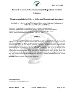
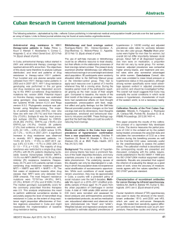
Figure 1: Histogram of the age at rst treatment for irradiated subjects.
The age at rst exposure A 1 is known for all individuals in the study. However, approximately 9% of the children had at least two irradiations (Table 1), and for those individuals
who were irradiated more than once, the age at which subsequent irradiation took place
is unknown, although it necessarily took place before the age of 16. Given the lack of information, we are forced to rely on a derived distribution for the ages of second and later
irradiations, as follows. In Figure 1 we give the age at rst irradiation histogram for irradiated subjects. Based on anecdotal evidence, we assumed that the age at second irradiation
was at least a year older than the age at rst irradiation. Using this, we set the age at second,
i
10
and if necessary subsequent irradiations as if they were a random sample from the histogram
in Figure 1 conditional on being at least a year older than the age at rst irradiation.
The ltration and nominal exposures depend on the machine and on the location. Table
2 shows what is known about where the irradiation took place. For example, a subject
whose irradiation code is "03" is known to have had one course of treatment at Haifa and
one course of treatment at Tel Hashomer, but it is not known which came rst. Table 4
shows the information known about prescribed skin exposure and ltration for the machines
used.
Percentage of
Prescribed
Place
all treatments Machine Filtration Exposure (R)
Haifa
72%
1
0.5
400
2
0.5
384
3
0.5
383
4
0.6
NA
Jerusalem
13%
1
0.5
425
2
0.5
425
3
0.5
425
Tel Hashomer
11%
1
0.0
350
2
0.0
350
"N"
1.6%
1
1.0
350{400
"Abroad"
1.9%
NA
NA
"Other"
0.8%
NA
NA
Table 4: Available information about machines used at the various treatment locations:
"NA" means not available. Notice that most treatments were performed in Haifa, and only
about 3% were performed in "N", "Abroad" or "Other".
In Jerusalem the machines had a common ltration 0:5 and nominal exposure 425. The
same occurs in Tel Hashomer, although the values of the ltration (0:0) and nominal exposure (350) diered from that in Jerusalem. In Haifa, there were four machines, with
ltrations (0:5; 0:5; 0:5; 0:6) and nominal exposures (400; 384; 383; NA), where NA means unknown, but the machine used on each child was not recorded. Thus, for Haifa we assumed
that the actual ltration was 0:5 with probability 0:75 and 0:6 with probability 0:25. For
the nominal exposure, we assumed that the distribution was 400, 384 and 383, each with
probability 0:25, while with probability 0:25 the nominal exposure was taken to be uniformly
11
Condition Label Nominal Exposure Re
Filtration F
C1
400
0.5
C2
384
0.5
C3
383
0.5
C4
Uniform[350,425]
0.6
C5
425
0.5
C6
350
0.0
C7
Uniform[350,425]
1.0
C8
Uniform[350,425] 0.0 with probability 0.10
0.5 with probability 0.85
1.0 with probability 0.05
Table 5: The distribution of ltration F and exposure R . The logarithm of the exposure
is assumed to be normally distributed with mean log(Re ) and standard deviation = 0:25.
Children exposed in Haifa are assumed to be in one of conditions C1 {C4 at random, each
with probability 0:25. For Jerusalem, the condition is C5 . For Tel Hashomer, the condition
is C6 . For location \N", the condition is C7 . For \other" and \abroad", the condition is C8 .
ij
ij
ij
r
distributed between 350 and 425, reecting the range of nominal exposures recorded in the
various centers. For those recorded as being in site "N", the ltration was 1:0 but the nominal exposure was unknown and again taken to be uniformly distributed between 350 and
425. Finally, for those who were irradiated abroad, neither ltration nor nominal exposure
were available. The nominal exposure was taken to be uniformly distributed between 350
and 425, while the ltration is assumed to take on the values (0:0; 0:5; 1:0) with probabilities (0:10; 0:85; 0:05), a distribution somewhat in keeping with the observed ltrations. We
describe the distributions of ltration and exposure in Table 5.
3.4 Expected Dose Given Available Information
The model developed above, and especially in Section 3.3 can be applied to compute expected
doses for individuals given available information. Let L be the number of irradiations for
person i. We need to compute E (D jX ; W ). The relevance of this quantity in the induced
hazard function given (X ; W ) is described in Section 4. Let D be the thyroid dose on
i
i
i
i
i
i
ij
12
treatment j . It follows of course that
E (D jX ; W ) =
i
i
i
X
XZ
E (D jX ; W ) =
E (D jX ; V )f (V jX ; W )dV :
=1
=1
Li
Li
i`
i
i
`
i`
i
i
i
i
i
i
`
40
30
20
1 course
2 courses
3 courses
4 courses
10
Estimate of E(Dose|Available Information) (cGy)
50
This quantity can be computed for each subject using the model for expected dose given
(X; V ) from Section 3.2, and the model for V given (X; W ) from Section 3.3. The integration
can be accomplished with Monte{Carlo methods, because in Section 3.3 we specied the
requisite distribution.
10
20
30
40
50
Previous Estimate of Dose (cGy)
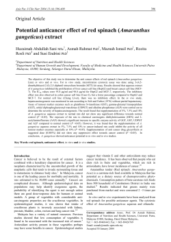
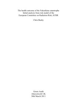
Figure 2: Plots of expected and mean doses given the observed data against the original
dose in the data base.
Values of E (DjX; W ) using the estimates of from the Modan, et al. data are plotted
versus the database estimates of dose in Figure 2. For the lower doses the mean is higher
than the database dose, primarily for the reasons discussed at the end of Section 3.2, i.e., the
mean of a skewed distribution is higher than the median. Another key feature of the plot
13
though is the curvature on the high end. This is due to our use of more realistic assumptions
about ages at second and subsequent exposures. The database dose used calculations that
assumed age at rst exposure for all courses of treatment, and therefore tended to be too
large because the calculations assumed that the subjects did not grow over time.
Table 6 compares the data base mean dose with the estimated doses from our dosimetry
model, on the basis of the number of treatments received.
Database
Model
Number of Number of average Average
courses
subjects
dose mean dose
0
16226
0.0
0.0
1
9814
8.4
9.8
2
904
17.5
18.6
3
110
25.7
26.4
4
6
27.0
28.1
Table 6: Basic statistics for the tinea capitis data base, and the results of the dosimetry.
Here \Database average dose" is the average dose as listed in the data base. \Model average
mean dose" is the average of the dose from the model, where the model dose is the mean
dose from the simulation.
4 LIKELIHOOD FORMULATION
4.1 Background and Introduction
The purpose of this section is to describe in detail the likelihood formulation we used to estimate the parameters in the model. Let D be true dose, V be a vector of variables available
for predicting dose from phantom studies (number of exposures, ages at all exposures, prescribed beam exposures in Roentgens at all exposures, added ltration in mm of aluminum
at all exposures), let W be a vector of variables available for predicting dose in the tinea
subjects (age at rst exposure, number of exposures, irradiation place code) and let X be a
vector of additional, observable covariables that may be present in the dose{response model
(sex, country of origin, age at rst exposure, number of exposures). Let T be the random
variable representing the elapsed time after entry into the study until onset of thyroid cancer.
14
The goal is to use the censored observations on T from the tinea capitis study group
to estimate the induced hazard function associated with the distribution of T given the
observables X and W , which will reveal the important features about the hazard function
of interest, namely the one associated with the distribution of T given D and X . The vector
V plays an intermediate role in this.
Let h(tjD; X; B) be the hazard function corresponding to the distribution of T conditional
on true dose and additional covariates X . We use (1) for the hazard function, which is a
commonly used model for dose-response at low doses of radiation.
4.2 Induced Hazard Function
Assume conditional independence of time to cancer and W , i.e.,
h(tjD; X; W ; B) = h(tjD; X; B):
(3)
It then follows from arguments analogous to those of Prentice (1982) that the induced hazard,
given X and W , has the form
h(tjX; W ; B; ) = E fh(tjD; X; B)jT
t; X; W ; g ;
(4)
where represents the unknown parameters in the distribution of D given X and W . It
is important to note that Prentice showed this to be true for the special case that W is a
measurement of D. In our case W is, instead, a vector of predictor variables. The derivation,
as shown in Section A.1 below, is identical to Prentice's, but the conditional independence
assumption (3) requires some dierent considerations.
In particular, the variable age at rst exposure is one component of W . On the surface,
therefore, it appears that we must assume that time to cancer is independent of age at rst
exposure when true dose is available; that is, we must assume there is no modifying eect
of exposure age in order to proceed. The situation is not so bad, though, since age at rst
exposure is also present in X . Apparently, the conditional independence assumption is only
that T is conditionally independent of those components of W that are not also present in
15
X.
Nevertheless, there must be some recognition that simultaneously accounting for dose
uncertainties and the modifying eect of exposure age may pose diÆculties, since exposure
age is one of the main variables that provides information about dose. The variable number
of exposures has similar problems. Since the risk of disease is small, the approximation to
(4) obtained by dropping the condition T t should be adequate (as discussed in Pepe et
al., 1989); in which case the hazard based on the observable covariates X and W is
h(tjX; W ; B; ) = E fh(tjD; X; B)jX; W ; g = h ftjE (DjX; W ; ); X; Bg ;
where the last equality holds because the assumed hazard function of interest is linear in
dose.
Thus, the parameters of interest are present in the hazard function given the observable
variables:
h(tjX; W ; B; ) = exp(X T (t)
br
br
h
i
) 1 + E (DjX; W ; ) expf + X T (t) g
dr
em
em
:
(5)
If, for example, is known and E (DjX; W ; ) can be calculated for each subject in
the tinea study group, then parameters may be estimated with standard methods but with
unknown doses replaced by their expectations given X and W . In general, the technique
of using usual methods but with the unknown doses replaced by their expectations given
available variables is known as regression calibration (Carroll, et al., 1995). There is additional justication here, though, since (5) is essentially the exact hazard function given the
available variables and not the result of a rst-order Taylor approximation for small dose
uncertainties.
If were known, then the parameters in the relative risk portion of (5), i.e., the part in
brackets, could be estimated either by the partial likelihood analysis of the Cox regression
model or by the subject-years method, which is based on Poisson likelihood calculations
of cancer occurrences tabulated over intervals of time after entry into the study. We shall
focus on the latter because we wish to use an exact likelihood function. In that way we can
16
combine the likelihood associated with the tinea subjects with the likelihood associated with
the phantom studies, in order to simultaneously estimate B and .
4.3 Likelihood function
The density function for T for the ith member of the tinea study group is
i
f (tjD; X ; B; ) = h(tjD ; X ; B) exp
i
i
Z
0
i
i
t
h(ujD; X ; B)du ;
i
i
where D is an abbreviation for E (D jX ; W ; ) and h(tjD; X ; B) is the hazard function
in (5) above, see, for example, Cox and Oakes (1984, Section 2.2). Assuming independence,
i.e., that the joint density of the T 's given expected doses and additional covariates is the
product of the individual densities, the log likelihood function from the tinea subjects is
h
n
o
i
given by ` (B; ) = P log h(T jD; X ; B) R0 h(ujD; X ; B)du , where is an
indicator variable for uncensored observations, and S is the minimum of T and the censoring
time (Cox and Oakes, 1984, Section 3.2).
The subject-years or Poisson approach oers relatively simple calculations by tabulation
according to various states that the subjects pass through during the course of observation.
For a given xed value of , the tinea data may be cross-classied according to J states
formed by all combinations of various categories of time since exposure and explanatory
variables such as sex, country of origin, expected dose and age at rst exposure. With
the inconsequential assumption that the covariables (X; D) take on constant values within
states, the loglikelihood reduces to
i
i
i
i
i
i
i
tinea
i
i
i
Si
i
i
i
i
i
`
tinea
(B; ) =
i
i
n
o
i
Xh
O log h(tjD ; X ; B) h(tjD ; X ; B)E ;
=1
J
j
j
j
j
j
j
(6)
j
where O is the observed number of cancers and E is the person-years of observation in
state j , see for example Breslow, et al. (1983). The actual value used for D, for a given ,
is the person-years weighted average of expected dose for all individuals i that observed in
state j .
j
j
j
17
One approach is to estimate from the phantom data, then treat it as known for maximum likelihood estimation of B from (6): we call this regression calibration. In this, however, the covariate Db is an imprecise estimate of the explanatory variable of interest, D.
Writing Db = D + , where represents the imprecision due to sampling variability in
estimating , it is evident that classical measurement error is present. Note, however, that
cov( ; ) 6= 0 because the error component b is common to all values.
Alternatively, we may combine the tinea likelihood with the likelihood from the phantom
studies and maximize them, with respect to (B; ) jointly: we call this calibrated likelihood.
Let `
() represent the log likelihood function from the phantom study. The combined
log likelihood is therefore
j
j
j
j
j
j
j
j
phantom
`
combined
(B; ) = `
n
o
i
Xh
() + O log h(tjD; X ; B) h(tjD; X ; B)E :
=1
J
phantom
j
j
j
j
j
j
(7)
j
This seems awkward in that the states j are dened for an unknown value of . Using a
Newton-Raphson or Fisher scoring algorithm for maximization, however, it is apparent that
the tabulations only need to be formed for current estimates of at each iteration.
4.4 Model for Expected Dose Given Proxy Variables
Recall that V represents the variables that are available for predicting dose from the phantom
studies but what we need is the expected value of dose given (X; W ), the variables available
on the tinea subjects. The connection between V and W is used in the following way:
E (DjX; W ; ) =
Z
E (DjX; V ; )f (VjX; W )dW :
(8)
The phantom data and dosimetric considerations lead to a model for E (DjX; V ; ). Details
of this are laid out in Section 3.
The distribution of V given (X; W ) depends on: (i) the distribution of ages at 2nd and
subsequent treatments given age at rst treatment (if applicable) and (ii) the distribution
of machine exposure (in Roentgens) and ltration given the subject's irradiation place code.
18
Details of the assumptions involved in this are laid out in Section 3. It is straightforward to
use Monte Carlo integration for (7).
It is now useful to insert the particular model derived from the phantom studies:
E (DjX; W ; ) = expf( 2
w
X
+ 2 + 2 )=2g g(A ; R ) exp(0 + 1 F 2);
=1
L
b
`
r
`
`
`
where L is the number of courses of treatment, A is the age at the time of the `th treatment,
R is the nominal skin exposure of the machine used in the `th treatment, F is the machine
ltration used in the `th treatment, and g() is a known function, see (2). So, using Monte
Carlo integration, take M samples from the distribution of V given (X; W ) and call these
V for m = 1; :::; M . Then we have as an approximation
`
`
`
m
XX
E (DjX; W ; ) M 1
expf(2 + 2 + 22 )=2gg(A ; R ) exp(0 + 1 F 2 ):
=1 =1
In the log likelihood function (6), D is the person-years weighted average of the doses
M
L
w
m
m;`
b
m;`
m;`
`
j
for all individuals represented in state j . Thus, for xed ,
X XX
D = M 1
w
2S =1 =1
M
L
i
j
i
j m
expf(2 + 2 + 2)=2gg(A
w
b
r
i;m;`
;R
i;m;`
) exp(0 + 1 F 2 ):
i;m;`
`
where S is the set of indices i corresponding to individuals whose exposure history includes
state j , w is the person-years of observation of individual i in state j as a proportion of the
total person-years of observation in state j .
The Fisher Scoring Algorithm may be used to nd the values of B and that maximize
(7).
j
i
5 THE REANALYSIS
In Section 4 we detailed two approaches for the analysis. In the regression calibration approach the "subject-years" or "Poisson" method is used to estimate the hazard function, but
with doses replaced by their expectations given available patient information; and with the
unknown parameter associated with the expectations, THETA, replaced by its estimate from
19
the phantom study. The cross-classication, in this case, was based on sex ( 2 levels); origin (3
levels: Africa, Asia, Israel); age at rst exposure (8 levels: [0,2),[2,4),[4,6),[6,8),[8,10),[10,12),
[12,14),[14,16)), attained age (8 levels: [0,15), [15,20), [20,25), [25,30), [30,35), [35,40),
[40,45), [45,)), and expected dose (6 levels: 0, (0,7.5), [7.5,15), [15,22.5), [22.5,30), [30,100)).
Attained age at time of thyroid cancer is the response here. Since the patients were all
exposed as children there is little dierence between using this response and time since exposure. In the calibrated likelihood approach the cross-classication is performed at each
iteration after an updating of the estimates of based on the combined data sets.
As seen in Table 7 the dierence in the estimates from these two approaches is very small
relative to the standard errors. Notice, though, that the standard error for the coeÆcient of
dose is larger in the calibrated likelihood estimate, as would be expected since this estimate
correctly incorporates the uncertainty in the estimate of . Neither approach, however,
incorporates the uncertainty in the estimates of the variances of the random eects.
The results in Tables 7 and 8, which are more suited for interpretation, are based on the
regression calibration approach. The results from Tables 7, 8 and 9 may be summarized as
follows:
1. There is a statistically signicant dose-response (1-sided p-value = 0.009). Although
the estimated modifying eect of age on the dose-response is pronounced, it is not
statistically signicant (2-sided p-value = 0.37).
2. Accounting for error in dosimetry changes hardly any of the parameter estimates, or
the relative risk for dierent ages at rst exposure.
3. There are a few technical points worth noting.
(a) We did not include sex as a modifying eect since, in all cases, its p-value is about
.4 (likelihood ratio test).
(b) The coeÆcients for background terms are not very interesting to us. Since these
20
do not depend on dose, we should expect to see what we did observe, namely
essentially no dierences in these for the various methods.
(c) These results are for ( ; ; ) = (0:17; 0:49; 0:15). We have redone the analysis
with ( ; ; ) = (0:17; 0:25; 0:25), and there is little change in the analysis.
(d) The value of the log likelihood from the phantom data alone is about -0:6. This
is essentially the amount by which the log likelihoods in the last two columns of
Table 7 dier.
w
w
b
b
r
r
6 DISCUSSION AND CONCLUSIONS
The uncertainties in thyroid radiation dose in the tinea capitis study are due to a variety of
factors, particularly the following.
1. Of course, radiation dose to the thyroid is unknown for all patients. In addition, there
are substantial amounts of missing data.
(a) Age at second+ exposure is missing for the 9% of the subject with more than one
exposure.
(b) The machines used, their ltration and the prescribed beam exposures to the
scalp are not known for many patients.
2. There are a variety of sources of Berkson{type errors.
(a) Within{individual eects, reecting the dierent thyroid doses that would occur
if a child were hypothetically irradiated twice under ideal conditions.
(b) Between{individual eects, reecting the dierent thyroid doses that would occur
for dierent children of identical rounded ages under ideal machine conditions,
due to dierences in head size and shape.
(c) Random errors due to dierences between prescribed and actual skin exposure.
21
3. There are some sources of classical measurement errors.
(a) The error model (2) includes two parameters, (0 ; 1), that control the relationship
between added ltration and dose, and these parameters are unknown and must
be estimated. When they are estimated from phantom studies, that act as a type
of classical measurement error, although shared among all individuals.
(b) The variances of the Berkson{type errors are unknown and must be estimated.
In principle, the error in this estimation is of the same classical{type as the error
in estimating (0 ; 1 ). Because these error variances are estimated with little
precision, we have chosen to perform a sensitivity analysis for them, nding little
sensitivity.
We have developed models that account for these uncertainties, and methods of estimation and inference for them. In particular, we developed the idea of a calibrated likelihood,
which is similar to the standard regression calibration or substitution algorithm, but which
uses the likelihood contribution about uncertainty parameters from external sources.
Our results were striking in nding little eect due to accounting for uncertainty. Parameter estimates, standard errors and inferences were all little aected by accounting for
the uncertainty. We believe this is due to the fact that the relative risk model (1) is linear
in dose, and because much of the uncertainty is of Berkson{type.
REFERENCES
Adamson, H. G. (1909). A simplied method of x{ray application for the cure of ringworm
of the scalp: Kienbock's method. Lancet, 1, 1378{1380.
Breslow, N. E., Lubin, J. H., Marek, P. & Langholz, B. (1983). Multiplicative models and
cohort analysis. Journal of the American Statistical Association, 78, 1{12.
Carroll, R. J., Ruppert, D. & Stefanski, L. A. (1995). Measurement Error in Nonlinear
Models. Chapman & Hall, London.
Cox, D. R. & Oakes, D. (1984). Analysis of Survival Data. Chapman & Hall, London.
Hu, P., Tsiatis, A. A. & Davidian, M. (1998). Estimating the parameters in the Cox model
when covariate variables are measured with error. Biometrics, 54, 1407{1409.
22
Hughes, M. D. (1993). Regression dilution in the proportional hazards model. Biometrics,
49, 1056{1066.
Lee, W. & Youmans, H. D. (1970). Doses to the central nervous system of children resulting
from x{ray therapy for tinea capitis. U.S. Department of Health, Education and Welfare,
Public Health Service Technical Report BRH/DBE, 70{74.
Lubin, J. H., Boice, J. D. & Samet, J. M. (1995). Errors in exposure assessment, statistical
power and the interpretation of residential radon studies. Radiation Research, 144, 329{
341.
Modan, B., Ron, E. & Werner, A. (1977). Thyroid cancer following scalp irradiation. Radiology, 123, 741{744.
Nakamura, T. (1992). Proportional hazards models with covariates subject to measurement
error. Biometrics, 48, 829{838.
Pepe, M. S., Self, S. G. & Prentice, R. L. (1989). Further results in covariate measurement
errors in cohort studies with time to response data. Statistics in Medicine, 8, 1167{1178.
Pierce, D. A., Stram, D. O. & Vaeth, M. (1990). Allowing for random errors in radiation
dose estimates for the atomic bomb survivors. Radiation Research, 123, 275{284.
Pierce, D. A., Stram, D. O., Vaeth, M., Schafer, D. (1992). Some insights into the errors in
variables problem provided by consideration of radiation dose{response analyses for the
A{bomb survivors. Journal of the American Statistical Association, 87, 351{359.
Ron, E., Lubin, J. H., Shore, R. E., Mabuchi, K., Modan, B., Pottern, L. M., Schneider,
A. B., Tucker, M. A. & Boice, J. D. (1995). Thyroid cancer after exposure to external
radiation: a pooled analysis of seven studies. Radiation Research, 141, 259{277.
Ron, E. & Homan, F. O. (1999). Uncertainties in Radiation Dosimetry and Their Impact
on Dose response Analysis. National Cancer Institute Press.
Ron, E., Modan, B., Preston, D., Alfandary, E., Stovall, M. & Boice, J. D. (1989). Thyroid
neoplasia following low{dose radiation in childhood. Radiation Research, 120, 516{531.
Rudemo, M., Ruppert, D. & Streibig, J. C. (1989). Random eect models in nonlinear
regression with applications to bioassay. Biometrics, 45, 349-362.
Schulz, R. J. & Albert, R. E. (1968). Follow{up study of patients treated by x{ray epilation
for tinea capitis III: dose to organs of the head from the x{ray treatment of tinea capitis.
Archives of Environmental Health, 17, 935{950.
Thomas, D., Stram, D. & Dwyer, J. (1993). Exposure measurement error: inuence on
exposure-disease relationships and methods of correction. Annual Review of Public
Health, 14, 69{93.
23
Werner, A., Modan B. & Davido, D. (1968). Doses to the brain, skull and thyroid following
x{ray therapy for tinea capitis. Phys. Med. Biol., 13, 247{258.
Appendix A
TECHNICAL DETAILS
A.1 Justication of (3)
As in Prentice (1982) and Pepe, et al. (1989), the hazard function induced by the observed
data is
pr(t T T + jX; W ; B)
h(tjX; W ; B) = lim
!0
Z pr(t T T + jD; X; W ; B; T t)f (DjX; W ; T t; )
dD
= lim
!0
Z
pr(t T T + jD; X; B; T t) f (DjX; W ; T t; )dD;
= lim
!0
this last step following from the conditional independence assumption (3). We have thus
shown that
h(tjX; W ; B) = E fh(tjD; X; B)jX; W ; T T; )g ;
as claimed.
24
Model With Age at Exposure
as Modifying Eect of Dose
Regression Calibrated
Naive Calibration Likelihood
Terms in Background Rate
constant
female indicator
Africa indicator
Israel indicator
attained age in [15,20)
attained age in [20,25)
attained age in [25,30)
attained age in [30,35)
attained age [35,inf)
Dose
Eect modier
age at exposure
Maximized log likelihood
Maximized log likelihood
without modifying eects
Dose without modifying eects
-11.94 (.65)
1.37 (.33)
-0.29 (.33)
-0.84 (.46)
1.05 (.56)
1.23 (.52)
1.32 (.51)
1.30 (.51)
1.34 (.58)
-0.38 (.57)
-11.95 (.65)
1.37 (.33)
-0.30 (.32)
-0.84 (.46)
1.05 (.56)
1.23 (.52)
1.32 (.51)
1.30 (.52)
1.34 (.58)
-0.53 (.57)
-11.94 (.65)
1.37 (.33)
-0.29 (.32)
-0.85 (.46)
1.04 (.56)
1.23 (.52)
1.32 (.51)
1.29 (.52)
1.33 (.58)
-0.52 (.58)
-0.12 (.09) -0.11 (.09) -0.11 (.09)
-598.0
-597.8
-598.4
-598.9
-598.6
-599.3
-1.05 (0.41) -1.18 (0.40) -1.17 (0.43)
Maximized log likelihood
without dose eects
-614.3
-614.3
-614.9
Table 7: Results for the dose{response model exp(X T )f1 + D exp( + X T )g. Parameter estimates are given, along with standard errors (in parentheses). There is obviously
little dierence between regression calibration and calibrated likelihood. The results are for
within{person standard deviation = 0:17, between{person standard deviation = 0:49,
and the standard deviation of random errors due to dierences between prescribed and actual
skin exposure = 0:15.
br
w
br
dr
em
em
b
r
Model
Age = 1 Age = 6 Age = 15
Naive
0.61
0.34
0.12
Corrected
0.53
0.30
0.11
Table 8: The relative risk depends on dose in the form 1 + Dose. This table gives the
estimates of for children with dierent ages at rst exposure.
25
Model
Naive
Age = 1 Age = 6 Age = 15
7.1
4.4
2.2
(3.2,17.6) (2.4,8.8) (1.2,9.7)
Corrected
6.3
4.0
2.1
(2.9,15.3) (2.2,8.2) (1.1,9.6)
Table 9: The estimated relative risk when children are exposed at a dose of 10cGy; 95%
condence intervals are given in parentheses.
26