NCSS Statistical Software
NCSS.com
Chapter 190
Box-Cox
Transformation
Introduction
This procedure finds the appropriate Box-Cox power transformation (1964) for a single batch of data. It is used to
modify the distributional shape of a set of data to be more normally distributed so that tests and confidence limits
that require normality can be appropriately used. It cannot correct every data ill. For example, data that contain
outliers may not be properly normalized by this technique.
Example of the Box-Cox λ Plot
190-1
© NCSS, LLC. All Rights Reserved.
NCSS Statistical Software
NCSS.com
Box-Cox Transformation
The Box-Cox transformation has the following mathematical form
𝑌𝑌 = (𝑋𝑋 + 𝛿𝛿)𝜆𝜆
where λ is the exponent (power) and δ is a shift amount that is added when X is zero or negative. When λ is zero,
the above definition is replaced by
𝑌𝑌 = ln(X + δ)
Usually, the standard λ values of -2, -1.5, -1, -0.5, 0, 0.5, 1, 1.5, and 2 are investigated to determine which, if any,
is most suitable. The program will also solve for the optimum value of λ using maximum likelihood estimation.
The program also calculates confidence limits about the optimum value. The usual procedure is to adopt the most
convenient standard value between the confidence limits. For example, if the confidence limits were 0.4 to 1.1, λ
would be set to the standard value of ‘1’ (no transformation) since this is the most convenient. Care must be used
when using the confidence limits, because they are heavily dependent on the sample size.
Box-Cox Algorithm
Suppose you have a sample of n response values X1, X2, …, Xn. Further suppose you visually determine a value of
δ the will keep all X + δ > 0. Calculate a set of Zi’s corresponding to the Xi’s using
�(𝑋𝑋 + 𝛿𝛿)𝜆𝜆 − 1�/�𝜆𝜆𝐻𝐻 𝜆𝜆−1 � 𝜆𝜆 ≠ 0
𝑍𝑍 = �
𝐻𝐻 ln(𝑋𝑋 + 𝛿𝛿)
𝜆𝜆 = 0
where H is the geometric mean of X + δ. That is,
𝑛𝑛
𝑛𝑛
𝐻𝐻 = ��(𝑋𝑋 + 𝛿𝛿)
𝑖𝑖=1
Scaling by H is intended to keep the standard deviation of the Z’s approximately the same as the standard
deviation of the X’s so that the standard deviations can be compared at various values of λ.
Maximum Likelihood Estimation of λ
In this case, the likelihood for a given λ is inversely proportional to the standard deviation of the corresponding
Z’s. The likelihood function is maximized when the standard deviation is minimized. A bracketing search
algorithm is conducted that continues to tighten the boundaries until a specified precision (bracket width) is
reached.
Approximate Confidence Interval for λ
An approximate confidence interval for λ is based on likelihood function which in turn is proportional to the
standard deviation (SD) of Z. The confidence limits correspond to the two values of λ at which
𝑆𝑆𝐷𝐷𝜆𝜆2 = 𝑆𝑆𝐷𝐷𝜆𝜆�2 exp �
𝜒𝜒12 (1 − 𝛼𝛼)
�
𝑛𝑛
where 𝜆𝜆̂ is the maximum likelihood estimate of λ and 𝜒𝜒12 (1 − 𝛼𝛼) is the percentage point of the chi-squared
distribution with one degree of freedom.
190-2
© NCSS, LLC. All Rights Reserved.
NCSS Statistical Software
NCSS.com
Box-Cox Transformation
Data Structure
The data may be entered as a single variable or as several variables that are joined together into one variable
during the analysis.
Procedure Options
This section describes the options available in this procedure.
Variables Tab
This panel specifies the variables used in the analysis.
Data Variables
Variable(s)
Specify one or more variables containing numeric values to be analyzed. The data in these variables will be
analyzed separately or combined depending on the setting of the Multiple Variables option below.
Multiple Variables
If more than one variable is specified, this option specifies whether these variables are analyzed separately or
jointly.
The options are
•
Perform a separate analysis...
A separate analysis is conducted for each variable.
•
Join all variables...
Join the data from all variables selected into one large variable that is then analyzed as if it were a single
variable.
Correction for Non-Positive Data Values
All values must be positive to use the Box-Cox transformation. When negative values are encountered, an amount
δ is added to each observation so that all resulting values are positive. This option controls if and how δ is
specified.
•
Do Nothing (δ = 0)
No corrective action is taken. Non-positive values will be treated as missing values.
•
Add a fixed amount δ to each data value
Specify a value for δ which will always be added.
•
Add δ = |Min| + 1% of Range to each data value
Automatically set δ equal to the mini8mum plus one percent of the data range. This will insure that the result
data values are always positive.
δ (Shift)
Specify an amount that will be added to each observation so that all values analyzed are positive. Hence, when
one or more values are negative, δ should be less than the absolute value of the data minimum.
Any values that are negative or zero after δ has been added are treated as missing values in the analysis.
190-3
© NCSS, LLC. All Rights Reserved.
NCSS Statistical Software
NCSS.com
Box-Cox Transformation
Maximum Likelihood Estimation of λ
Search for λ from Minimum to Maximum
The maximum likelihood estimate of λ is found using a special search algorithm that looks between two
boundaries for the optimum value. Set the minimum boundary and the left and the maximum boundary on the
right.
Typically, λ is between -5 and 5, so the minimum is often set to -5 and the maximum is often set to 5.
Width Around λ is Less Than
The search for the optimum value of λ uses a simple bracketing strategy. As the algorithm progresses, the distance
between the upper and lower boundaries is decreased. Once this distance is less than the amount specified here,
the algorithm is considered to have converged.
The scale is in terms of λ. Since λ is usually rounded to the nearest half, a precision of 0.001 will be more than
adequate.
Width Around C.L. is Less Than
The search for the confidence limits of the optimum λ uses a simple bracketing strategy. As the algorithm
progresses, the distance between the upper and lower boundaries is decreased. Once this distance is less than the
amount specified here, the algorithm is considered to have converged.
The scale is in terms of the standard deviation of Y (X + δ). In most cases, a value of 0.0001 will be more than
adequate.
Number of Iterations is More Than
Specify the maximum number of iterations used in the search for the optimum λ and in the search for the
confidence limits about that optimum λ.
Usually, the algorithm will converge in 20 to 30 iterations, so we recommend 50 just to be on the safe side.
Standard λ’s (Shown on Reports and Plots)
Input Type
Specify the input format of the standard λ values.
•
Range of λ values
Enter the minimum, maximum, and interval width from which a set of λ’s may be calculated.
•
List of λ values
Specify a list of λ’s directly.
Generate λ’s from Min to Max
Enter the minimum and maximum values of λ. A set of λ’s between the minimum and maximum is generated at
points indicated by the Interval parameter. The maximum value is always included in the set, even if it does not
match perfectly with the minimum and interval width.
The scaled standard deviation and normality test probability level are reported for each λ. Note that λ is the power
(exponent) of the variable transformation. If λ is zero, the logarithmic transformation is used. Usually, λ is
between -3 and 3.
Example
The settings minimum = 0, maximum = 2.5, and interval = 1 generates the set
0 1 2 2.5
190-4
© NCSS, LLC. All Rights Reserved.
NCSS Statistical Software
NCSS.com
Box-Cox Transformation
Interval
Enter the interval between successive λ values. Typically, the interval is set to 0.5 or 0.25. Other values may be
used, but most authors recommend either 0.5 or 0.25.
This value must be a positive number (zero is not allowed).
List of λ Values
Enter a list of λ values separated by blanks or commas. The scaled standard deviation and normality test
probability level are displayed for each λ in the list.
Usually, λ is between -3 and 3.
Examples
-3 -2 -1 -0.5 0 0.5 1 2 3
-3 -2 -1 -0.5 -0.1
0 0.5 1 2 3
Reports Tab
The following options control the formatting of the reports.
Select Reports
Run Summary
Check to display this report.
Optimum λ and Confidence Limits
Check to display this report.
Standard λ’s
Check to display this report.
Confidence Intervals
Confidence Level
Enter the confidence level of the confidence interval for the optimum λ. This value is entered as a percentage
between 50 and 99.99. Usually, 95 is entered.
Reports Options Tab
The following options control the formatting of the reports.
Report Options
Variable Names
This option lets you select whether to display variable names, variable labels, or both.
190-5
© NCSS, LLC. All Rights Reserved.
NCSS Statistical Software
NCSS.com
Box-Cox Transformation
Decimal Places
λ’s – Test Statistics
These options allow you to specify the number of decimal places directly or based on the significant digits. If one
of the Auto options is used, the ending zero digits are not shown. For example, if ‘Auto (Up to 7)’ is chosen,
0.0500 is displayed as 0.05, 1.314583689 is displayed as 1.314584
The output formatting system is not always designed to accommodate ‘Auto (Up to 13)’, and if chosen, this will
likely lead to lines that run on to a second line. This option is included, however, for the rare case when a very
large number of decimals is needed.
Plots Tab
These options let you specify which plots are displayed.
Select Plots
Histogram of Original Data
Check to output this histogram.
Histogram of using Optimum λ
Check to output this histogram.
Histogram of using Standard λ’s
Check to output these histograms.
Histogram Format
Click this button to specify the format of these histograms. A plot using sample data (not your actual data) will be
displayed. If you would like to edit the plot with your actual data loaded into the plot preview, check the Edit
During Run box in the upper right-hand corner of the plot format button.
Probability Plot of Original Data
Check to output this probability plot.
Probability Plot of using Optimum λ
Check to output this probability plot.
Probability Plot of using Standard λ’s
Check to output these probability plots.
Probability Plot Format
Click this button to specify the format of these probability plots. A plot using sample data (not your actual data)
will be displayed. If you would like to edit the plot with your actual data loaded into the plot preview, check the
Edit During Run box in the upper right-hand corner of the plot format button.
λ vs SD Plot
Check to output this plot.
λ vs SD Plot Format
Click this button to specify the format of this plot. A plot using sample data (not your actual data) will be
displayed. If you would like to edit the plot with your actual data loaded into the plot preview, check the Edit
During Run box in the upper right-hand corner of the plot format button.
190-6
© NCSS, LLC. All Rights Reserved.
NCSS Statistical Software
NCSS.com
Box-Cox Transformation
Plots Options Tab
These options let you specify where to store various row-wise statistics.
Decimal Places for Plot Titles and Label
λ in Labels and Titles
These options allow you to specify the number of decimal places directly or based on the significant digits. If one
of the Auto options is used, the ending zero digits are not shown. For example, if ‘Auto (Up to 7)’ is chosen,
0.0500 is displayed as 0.05 and 1.314583689 is displayed as 1.314584.
δ in Labels and Titles
These options allow you to specify the number of decimal places directly or based on the significant digits. If one
of the Auto options is used, the ending zero digits are not shown. For example, if ‘Auto (Up to 7)’ is chosen,
0.0500 is displayed as 0.05.
Text for Plot Titles and Label
λ vs SD Plot Title Line 1 – Legend - Standard
Enter the text to be used in plot titles, labels, and legends.
The following substitutions will take place as the entered text is processed.
{Z} will be replaced by the current variable name (or names).
{D} will be replaced by the current value of δ.
190-7
© NCSS, LLC. All Rights Reserved.
NCSS Statistical Software
NCSS.com
Box-Cox Transformation
Example 1 – Box-Cox Transformation of Brain Weights
This section presents an example of how to run a Box-Cox transformation analysis of the brain weights of 15
types of mammals. The data used are found in the Mammals dataset.
You may follow along here by making the appropriate entries or load the completed template Example 1 by
clicking on Open Example Template from the File menu of the procedure window.
1
Open the Mammals dataset.
•
From the File menu of the NCSS Data window, select Open Example Data.
•
Click on the file Mammals.
•
Click Ok.
2
Open the Box-Cox Transformation window.
•
On the menus, select Analysis, then Descriptive Statistics, then Box-Cox Transformation. The BoxCox Transformation procedure will be displayed.
•
On the menus, select File, then New Template. This will fill the procedure with the default template.
3
Specify the variables.
•
On the Box-Cox Transformation window, select the Variables tab.
•
Double-click in the Variable(s) box. This will bring up the variable selection window.
•
Select Brain_Weight from the list of variables and then click Ok. Brain_Weight will appear in the
Variables box.
•
That’s it. All other options can stay at their default values.
4
Run the procedure.
•
From the Run menu, select Run Procedure. Alternatively, just click the green Run button.
Run Summary Section
Run Summary for Brain_Weight
Parameter
δ (Shift)
Optimum λ (Power)
Minimum λ Searched
Maximum λ Searched
Target Search Width of λ
MLE Iterations Used
Max MLE Iterations
Value
0
-0.0899
-5
5
0.0001
26
50
Parameter
Rows Processed
Rows Used
Rows Positive (with δ)
Value
15
15
15
Geometric Mean (with δ)
Minimum
Maximum
326.7287
26.0000
5712.0000
This report summarizes the run by showing main results as well as the input settings that were used. You should
pay particular attention to the Rows lines to make sure that they are as you expect. Also, if the number of MLE
Iterations is equal to the Max MLE Iterations, the search algorithm may not have converged properly.
190-8
© NCSS, LLC. All Rights Reserved.
NCSS Statistical Software
NCSS.com
Box-Cox Transformation
Optimum (Maximum Likelihood) Estimate of λ
Optimum (Maximum Likelihood) Estimate of λ for X = Brain_Weight
Power Transformation: Y = (X + δ) ^ λ
Standard
Shapiro-Wilk
Deviation
Normality
Power
Shift
of Y =
Test
Item
λ
δ
(X + δ) ^ λ
Statistic
Optimum (MLE)
-0.0899
0
501.4511
0.9726
Lower 95% C. L.
-0.4211
0
569.9324
0.9165
Upper 95% C. L.
0.2294
0
569.9583
0.8950
Shapiro-Wilk
Prob Level
0.8946
0.1700
0.0800
This report gives the results for the maximum likelihood estimation portion of the analysis.
Item
The name of item being reported on this line of the report.
Power λ
The value of λ for this item. This is the transformation exponent.
Shift δ
The value of δ, the shift value.
Standard Deviation of Y = (X + δ) ^ λ
This is the standard deviation of the transformed data values. Actually, the data have not only been shifted and
raised to the indicated power, but they have also been scaled by the geometric mean so that the standard
deviations are directly comparable. Note the geometric mean is not used when using the λ that has been found by
this algorithm.
Shapiro-Wilk Normality Test Statistic
The value of the Shapiro-Wilk normality test statistic calculated on transformed data.
Shapiro-Wilk Prob Level
The probability level of the Shapiro-Wilk normality test. Since the desire is to transform the data to be more
normally distributed, you are looking for large (non-significant) values. Remember that this value is not only
influenced by the normality of the data, but also by the sample size.
Standard λ’s
Standard λ’s for X = Brain_Weight
Power Transformation: Y = (X + δ) ^ λ
Item
1
2
3
4
5
6
7
8
Power
λ
-2.0000
-1.0000
-0.5000
0.0000
0.5000
1.0000
1.5000
2.0000
Shift
δ
0
0
0
0
0
0
0
0
Standard
Deviation
of Y =
(X + δ) ^ λ
6717.1155
1117.7134
607.4627
506.5852
761.9966
1733.7314
4804.2570
14744.4980
Shapiro-Wilk
Normality
Test
Statistic
0.4763
0.7051
0.8896
0.9640
0.7694
0.5836
0.4961
0.4583
Shapiro-Wilk
Prob Level
0.0000
0.0003
0.0661
0.7615
0.0015
0.0000
0.0000
0.0000
λ's between the maximum likelihood confidence limits are bolded.
This report displays the results for each of the standard λ’s.
190-9
© NCSS, LLC. All Rights Reserved.
NCSS Statistical Software
NCSS.com
Box-Cox Transformation
Item
The number of item being reported on this line of the report.
Power λ
The value of λ for this item. This is the transformation exponent.
Shift δ
The value of δ, the shift value.
Standard Deviation of Y = (X + δ) ^ λ
This is the standard deviation of the transformed data values. Actually, the data have not only been shifted and
raised to the indicated power, but they have also been scaled by the geometric mean so that they standard
deviations are directly comparable. Note the geometric mean is not used when using the λ that has been found by
this algorithm.
Shapiro-Wilk Normality Test Statistic
The value of the Shapiro-Wilk normality test statistic calculated on transformed data.
Shapiro-Wilk Normality Prob Level
The probability level of the Shapiro-Wilk normality test. Since the desire is to transform the data to be more
normally distributed, you are looking for large (non-significant) values. Remember that this value is not only
influenced by the normality of the data, but also by the sample size.
Plots
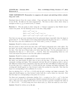
Plot for Choosing λ
This plot gives a visual representation that will help you select the value of λ that you want to use. The optimum
value found by maximum likelihood is plotted with a large, red asterisk. This value is usually inconvenient to use,
so a convenient (standard) value is sought for that is close to the optimum value. These convenient values are
plotted using a blue circle with a red center. In this example, it is obvious that λ = 0 is certainly a reasonable
choice. The large shaded area in the middle of the plot highlights the values of λ that are within the confidence
interval for the optimum.
190-10
© NCSS, LLC. All Rights Reserved.
NCSS Statistical Software
NCSS.com
Box-Cox Transformation
Note that this plot was created using the Scatter Plot procedure. The shading effects and different plot symbols
were made by making several groups of data.
Plot for Assessing Normality at Various λ’s
These plots let you see the improvement towards normality achieved by the power transformation. The top row
shows the histogram and probability plot of the original data. The lack of normality is evident in the two plots.
The bottom row shows the same two plots applied to the data that has been transformed by the optimum λ. They
are now much closer to being normally distributed.
190-11
© NCSS, LLC. All Rights Reserved.