
- Astronomy & Astrophysics
Astronomy
&
Astrophysics
A&A 573, A137 (2015)
DOI: 10.1051/0004-6361/201424924
c ESO 2015
Compton thick AGN in the XMM-COSMOS survey
G. Lanzuisi1,2 , P. Ranalli1 , I. Georgantopoulos1 , A. Georgakakis1,3 , I. Delvecchio2,4 , T. Akylas1 , S. Berta3 ,
A. Bongiorno5 , M. Brusa2,4 , N. Cappelluti2 , F. Civano6 , A. Comastri2 , R. Gilli2 , C. Gruppioni2 , G. Hasinger7 ,
K. Iwasawa8,9 , A. Koekemoer10 , E. Lusso11 , S. Marchesi4,6 , V. Mainieri12 , A. Merloni3 , M. Mignoli2 , E. Piconcelli5 ,
F. Pozzi2,4 , D. J. Rosario3 , M. Salvato3 , J. Silverman13 , B. Trakhtenbrot14, , C. Vignali2,4 , and G. Zamorani2
1
2
3
4
5
6
7
8
9
10
11
12
13
14
Institute of Astronomy & Astrophysics, National Observatory of Athens, Palaia Penteli, 15236 Athens, Greece
e-mail: [email protected]
INAF – Osservatorio Astronomico di Bologna, via Ranzani 1, 40127 Bologna, Italy
Max-Planck-Institut für extraterrestrische Physik, Giessenbachstrasse, 85748 Garching, Germany
Dipartimento di Fisica e di Astronomia, Universitá di Bologna, via Ranzani 1, 40127 Bologna, Italy
INAF – Osservatorio Astronomico di Roma, via Frascati 33, 00040 Monte Porzio Catone (RM), Italy
Yale Center for Astronomy and Astrophysics, 260 Whitney Avenue, CT 06520 New Haven, USA
Institute for Astronomy, 2680 Woodlawn Drive, HI 96822-1839 Honolulu, USA
ICREA and Institut de Ciències del Cosmos, Universitat de Barcelona, IEEC-UB, Martí i Franquès, 1, 08028 Barcelona, Spain
Institut de Ciéncies del Cosmos (ICCUB), Universitat de Barcelona, Martí i Franqués, 1 08028 Barcelona, Spain
Space Telescope Science Institute, 3700 San Martin Drive, MD 21218 Baltimore, USA
Max Planck Institut fur Astronomie, Königstuhl 17, 69117 Heidelberg, Germany
European Southern Observatory, Karl-Schwarzschild-Strasse 2, 85748 Garching, Germany
Kavli Institute for the Physics and Mathematics of the Universe (IPMU) 5-1-5 Kashiwanoha Kashiwa, 277-8583 Chiba, Japan
Department of Physics, Institute for Astronomy, ETH Zurich, Wolfgang-Pauli-Strasse 27, 8093 Zurich, Switzerland
Received 5 September 2014 / Accepted 25 November 2014
ABSTRACT
Heavily obscured, Compton thick (CT, NH > 1024 cm−2 ) active galactic nuclei (AGN) may represent an important phase in
AGN/galaxy co-evolution and are expected to provide a significant contribution to the cosmic X-ray background at its peak. However,
unambiguously identifying CT AGN beyond the local Universe is a challenging task even in the deepest X-ray surveys, and given
the expected low spatial density of these sources in the 2−10 keV band, large area surveys are needed to collect sizable samples. Through direct X-ray spectra analysis, we selected 39 heavily obscured AGN (NH > 3 × 1023 cm−2 ) at bright X-ray fluxes
−14
−1
−2
2
(F2−10 >
∼ 10 erg s cm ) in the 2 deg XMM-COSMOS survey. After selecting CT AGN based on the fit of a simple absorbed
two power law model to the shallow XMM-Newton data, the presence of bona fide CT AGN was confirmed in 80% of the sources
using deeper Chandra data and more complex models. The final sample comprises ten CT AGN (six of them also have a detected
Fe Kα line with EW ∼ 1 keV), spanning a wide range of redshifts (z ∼ 0.1−2.5) and luminosity (L2−10 ∼ 1043.5 −1045 erg s−1 ) and is
complemented by 29 heavily obscured AGN spanning the same redshift and luminosity range. We collected the rich multi-wavelength
information available for all these sources, in order to study the distribution of super massive black hole and host properties, such as
black hole mass (MBH ), Eddington ratio (λEdd ), stellar mass (M∗ ), specific star formation rate (sSFR) in comparison with a sample
of unobscured AGN. We find that highly obscured sources tend to have significantly smaller MBH and higher λEdd with respect to
unobscured sources, while a weaker evolution in M∗ is observed. The sSFR of highly obscured sources is consistent with the one
observed in the main sequence of star forming galaxies, at all redshifts. We also present and briefly discuss optical spectra, broadband
spectral energy distribution (SED) and morphology for the sample of ten CT AGN. Both the optical spectra and SED agree with
the classification as highly obscured sources: all the available optical spectra are dominated by the stellar component of the host
galaxy, and to reproduce the broadband SED, a highly obscured torus component is needed for all the CT sources. Exploiting the high
resolution Hubble-ACS images available, we are able to show that these highly obscured sources have a significantly larger merger
fraction with respect to other X-ray selected samples of AGN. Finally we discuss the implications of our findings in the context of
AGN/galaxy co-evolutionary models, and compare our results with the predictions of X-ray background synthesis models.
Key words. galaxies: nuclei – galaxies: Seyfert – quasars: general – X-rays: galaxies
1. Introduction
Observational and theoretical arguments suggest that the obscured phase of super massive black hole (SMBH) growth
holds important information on both the accretion history of the
Appendices are available in electronic form at
http://www.aanda.org
Zwicky postdoctoral fellow.
Universe and the interplay between active galactic nuclei (AGN)
and their host galaxies. Obscured AGN for example, are essential for reconciling the mass function of black holes in the local
Universe with that expected from AGN relics, i.e. inferred by
integrating the luminosity function of AGN via the continuity
equation (e.g. Soltan 1982; Marconi et al. 2004). The spectral
shape of the diffuse X-ray background also requires a large number of mildly obscured AGN (Gilli et al. 2007) and even possibly deeply buried ones with column densities in excess of the
Article published by EDP Sciences
A137, page 1 of 23
A&A 573, A137 (2015)
24
−2
Compton thick limit (CT AGN, NH >
∼ 10 cm ; Treister et al.
2009; Akylas et al. 2012).
X-ray surveys provide a relatively unbiased census of the
accretion history in the Universe, as they can penetrate large
amounts of dust and gas, especially in the hard, 2−10 keV
band. X-ray surveys indeed find that the accretion density of the
Universe is dominated by black holes that grow their mass behind large columns of dust and gas clouds (e.g. Mainieri et al.
2002; Ueda et al. 2003; Tozzi et al. 2006; Akylas et al. 2006;
Buchner et al. 2014; Ueda et al. 2014).
However, the exact intrinsic fraction of CT AGN remains
highly uncertain, ranging from about 10% of the total AGN population up to 35%. Owing to ultra-hard X-ray surveys above
10 keV performed with Swift and INTEGRAL, CT AGN are
commonly observed in the local Universe, representing up
to 20% of local active galaxies at energies 15−200 keV down
to a flux limit of 10−11 erg cm−2 s−1 (see Burlon et al. 2011, and
references therein). Still, the identification of CT AGN beyond
the local universe is challenging. Recent results on preliminary
NuSTAR (Harrison et al. 2013) data were only able to put an upper limit (<33%) to the fraction of CT AGN between z = 0.5−1
(Alexander et al. 2013).
Within the AGN/galaxy co-evolution perspective, dust and
gas enshrouded AGN represent an evolutionary point that is critical for understanding how the growth of black holes relates
to the build-up of the stellar populations of their hosts. The
generic picture proposed involves gas inflows triggered by internal (Hopkins & Hernquist 2006; Ciotti & Ostriker 1997, 2007;
Bournaud et al. 2011; Gabor & Bournaud 2013) or external
(Sanders et al. 1988; Di Matteo et al. 2005; Hopkins et al.
2006) processes. These result in a period of rapid black hole
growth that takes place within dense dust and gas cocoons. It
is then followed by a blow-out stage during which some form
of AGN feedback depletes the gas reservoirs thereby regulating both the star-formation and black hole growth. The study of
obscured AGN has the potential to provide important pieces of
the puzzle, such as the nature of the triggering mechanism, the
physics of AGN outflows and their impact on the host galaxy.
The evidence above motivated numerous studies to identify
the most heavily obscured AGN, determine their space density
relative to unobscured sources and study their host galaxy properties (e.g. Hickox et al. 2009; Brusa et al. 2009; Mainieri et al.
2011; Donley et al. 2012; Rovilos et al. 2014; Delvecchio et al.
2014). At X-rays in particular, there has been an explosion recently in the quality and quantity of data available, a development that led to direct constraints on the fraction of even the
most deeply shrouded CT sources over a wide range of redshifts
(e.g. Tozzi et al. 2006; Burlon et al. 2011; Comastri et al. 2011;
Brightman & Ueda 2012; Georgantopoulos et al. 2013; Buchner
et al. 2014; Brightman et al. 2014). Despite significant progress,
there are still differences in the heavily obscured AGN samples
compiled by different groups using the same data. This is primarily related to variations in the spectral analysis methods, e.g.
the complexity of the X-ray spectral models adopted or how uncertainties due to photometric redshifts or the Poisson nature of
X-ray spectra are propagated in the analysis. It has been shown
for example, that a common feature of obscured AGN spectra
is emission at soft energies in excess to the primary continuum, possibly due to scattered radiation into the line of sight
(Brightman & Nandra 2012; Buchner et al. 2014). Taking this
component into account is clearly important for identifying the
most obscured AGN in X-ray surveys. Recently, Buchner et al.
(2014) also demonstrated the importance of advanced statistical
methods that properly account for various sources of uncertainty,
A137, page 2 of 23
allow robust X-ray spectral parameter estimation and hence, the
identification of secure heavily obscured AGN samples.
In this paper we search for the most heavily obscured AGN
in the COSMOS field (Scoville et al. 2007) starting from the
XMM-COSMOS catalog (Hasinger et al. 2007; Cappelluti et al.
2009) and using deeper Chandra data (Elvis et al. 2009) to test
the efficiency of our selection method for CT AGN. Moreover,
using the wealth of multi-wavelength data available in the
COSMOS field, we explore the accretion and host galaxy properties of the obscured AGN sample, in order to place them in
the context of AGN-Galaxy co-evolution scenarios. This stage
should be characterized by small BH masses, high accretion and
star formation (SF) rates (e.g. Fabian 1999; Page et al. 2004;
Draper & Ballantyne 2010), and could be possibly merger-driven
(Hopkins et al. 2008). Our multi-wavelength analysis attempts
to provide constraints on such models. Finally we present an
atlas of the multi-wavelength properties (i.e. broadband SED,
optical spectra, morphology) of the sample of 10 bona fide
CT AGN. Throughout the paper, a standard Λ−CDM cosmology with H0 = 70 km s−1 Mpc−1 , ΩΛ = 0.7 and ΩM = 0.3 is
used. Errors are given at 90% confidence level.
2. The dataset
2.1. Multi-wavelength coverage in the COSMOS field
One of the main goals of the Cosmic Evolution Survey
(COSMOS; Scoville et al. 2007) is to trace star formation
and nuclear activity along with the mass assembly history of
galaxies as a function of redshift. The 2 deg2 area of the
HST COSMOS Treasury program is bounded by 9h 57.5m <
RA < 10h 03.5m ; 1◦ 27.50 < Dec < 2◦ 57.50. The field
has a unique deep and wide multi-wavelength coverage, from
the optical band (Hubble, Subaru, VLT, and other groundbased telescopes), to the infrared (Spitzer, Herschel), X-ray
(XMM-Newton and Chandra) and radio (Very Large Array
(VLA) and future Jansky-VLA, P.I. V. Smolcic) bands. Large
dedicated ground-based spectroscopy programs in the optical
with Magellan/IMACS (Trump et al. 2009), VLT/VIMOS (Lilly
et al. 2009), Subaru-FMOS (P.I. J. Silverman), and DEIMOSKeck (P.I. N. Scoville) have been completed or are well under
way. Very accurate photometric redshifts are available for both
the galaxy population (Δz/(1+z) < 1%; Ilbert et al. 2009) and the
AGN population (Δz/(1 + z) ∼ 1.5% Salvato et al. 2009, 2011).
The COSMOS field has been observed with XMM-Newton
for a total of ∼1.5 Ms at a rather homogeneous depth of ∼60 ks
(Hasinger et al. 2007; Cappelluti et al. 2009). The XMM-Newton
catalog used in this work includes ∼1800 point-like sources, detected in one or more of the 3 adopted bands (0.5−2, 2−10 and
5−10 keV), and having a hard (2−10 keV) band limiting flux of
2.5 × 10⁻¹⁵ erg cm−2 s−1 (and 5.6(9.3) × 10−15 erg cm−2 s−1 on
50% (90%) of the area). The adopted likelihood threshold corresponds to a probability of ∼4.5 × 10⁻⁵ that a catalog source
is a spurious background fluctuation. 197 sources are classified
as stars or unclassified (Brusa et al. 2010), so they are excluded
from the following X-ray spectral analysis.
At the hard band flux limit of the XMM-COSMOS survey,
current CXB models predict a fraction of CT-AGN between 1
and 3% (Gilli et al. 2007; Treister et al. 2009; Ueda et al. 2014),
while at a flux limit of F2−10 ∼ 10−14 erg cm−2 s−1 , above which
a basic spectral analysis is viable, this fraction is even smaller
(<
∼1%, see Sect. 8). Therefore, the XMM-COSMOS catalog may
seem not the best place where to look for, in order to select a
large sample of CT AGN, even taking into account the large area
G. Lanzuisi et al.: Compton thick AGN in the XMM-COSMOS survey
covered. However, the great advantage of the XMM-COSMOS
dataset is that there are deeper X-ray observations available in
the same area: the Chandra-COSMOS and its new extension,
COSMOS legacy (Elvis et al. 2009; Civano et al. 2014), that
together cover the same 2 deg2 area of the XMM-Newton observation, with a homogeneous exposure time of ∼160 ks (flux
limit F2−10 ∼ 7 × 10⁻¹⁶ erg cm−2 s−1 ). This will allow us to use
the deeper X-ray data to evaluate, a posteriori, the efficiency of
our XMM-based CT AGN selection method (see Sect. 4.1), with
the final goal to extend, in the future, these studies to the deeper
full Chandra catalog in COSMOS. Given the difficulty of unambiguously identifying CT AGN beyond the local Universe, this
is a valid alternative approach to simulations, to evaluate the efficiency of the selection method.
Furthermore, a great wealth of information has been made
available in the latest years, regarding multi-wavelength, host
and SMBH properties of the sources in the XMM-COSMOS catalog: Trump et al. (2009), Merloni et al. (2010) and Rosario et al.
(2013) present SMBH masses for large samples of type-1 AGN
(182, 89 and 289, respectively, the latter computed from a compilation of all the spectra available); Mainieri et al. (2011)
present multi-wavelength properties of 142 obscured QSOs;
Bongiorno et al. (2012, B12 hereafter) present host properties
(star formation rate, stellar mass etc.) of a sample of 1700 AGN;
Lusso et al. (2012, L12 hereafter) present bolometric luminosities and Eddington ratios of a sample of 929 AGN, both
type-1 and type-2, and SMBH masses estimated trough scaling relations for 488 type-2 AGN. Delvecchio et al. (2014, D14
hereafter) performed broadband SED decomposition for all the
160 μm Herschel detected COSMOS sources. The availability
of all this information is crucial in order to study the role of
CT AGN in the context of AGN/galaxy co-evolution.
2.2. Sample selection
The XMM-Newton spectra have been extracted as described in
Mainieri et al. (2007). The original spectral extraction was performed only for the EPIC pn-CCD (pn) camera (Struder et al.
2001). All the spectral fits are performed with Xspec v. 12.7.1
(Arnaud et al. 1996). We analyzed the 1625 X-ray pn spectra
of the identified extragalactic sources, using the same automated
fit procedure presented in Lanzuisi et al. (2013a). This procedure
makes use of the C-statistic (Cash 1979), especially developed to
model spectra with a small number of counts. It requires the simultaneous fit of the background (BKG) and very limited counts
binning (minimum of 1 counts per bin, in order to avoid empty
channels).
The global XMM-Newton pn background between 0.3 and
10 keV is complex, and comprises an external, cosmic BKG,
passing through the telescope mirrors, and therefore convolved
with the instrumental Auxiliary Response File (ARF), and the
internal, particle induced BKG, which is not convolved by the
ARF. The external BKG, which dominates at soft energies (below ∼1 keV) is modeled with two thermal components (Xspec
model APEC), with solar abundances, one for the local hot bubble (kT ∼ 0.04 keV) and the second for the Galactic component
(kT ∼ 0.12 keV), produced by the ISM of the Galactic disk
(Kuntz & Snowden 2000), plus a power-law reproducing the
Cosmic X-ray Background (Γ ∼ 1.4), mostly due to unresolved
discrete sources (Comastri et al. 1995; Brandt et al. 2002). The
particle induced BKG is well reproduced by a flat power-law
(Γ ∼ 0.5), plus several strong emission lines at energies of 1.5,
7.4, 8.0 and 8.9 keV, due to Al, Ni, Cu and Zi+Cu Kα lines,
respectively (Freyberg et al. 2004).
We adopted as source model a simple double power-law:
the primary power-law, modified by intrinsic absorption at the
source redshift, representing the transmitted component, plus a
second power-law to account for the soft emission commonly
observed in local highly obscured sources (e.g. Done et al.
2003). This emission can be due to unobscured flux leaking
out in the soft band (through scatter or partial covering), thermal emission related to star-formation, or the blend of emission lines from photo-ionized circumnuclear gas (Guainazzi &
Bianchi 2007) or a combination of these components. Given the
relatively poor photon statistics and the lack of high spectral resolution, distinguishing between these different origins is not possible here, and the second power-law is only used as a simple
description of the observed spectra in the soft band. However,
the presence of a second, soft component is essential in order
to recover a correct estimate of the intrinsic absorption affecting
the primary power-law, especially for highly obscured sources
(Brightman et al. 2014; Buchner et al. 2014).
The normalization of the soft component is constrained to
be less than 10% with respect to the hard component. In wellstudied nearby AGN, a small percentage is the typical flux
contribution of the soft component with respect to the unobscured primary one (e.g. Turner et al. 1997). The photon index of the soft component is linked to that of the primary
power-law, in order to minimize the number of free parameters.
Both power-laws are absorbed by a Galactic column density of
1.7 × 1020 cm−2 (Kalberla et al. 2005), observed in the direction of the COSMOS field1 . The energy range in which the fit is
performed is 0.3−10 keV.
We note that the minimum number of counts for which this
kind of analysis can be applied is constrained only by the maximum relative error that one wants to allow for the free parameters in the fit. Because here we are mainly interested in recovering the intrinsic absorption and luminosity of our sources,
we fixed the photon index Γ to 1.9 for sources with fewer than
100 net counts (70% of the sources have fewer than 100 counts).
This value is the one typically found in AGN at any luminosity
level (Nandra & Pounds 1994; Piconcelli et al. 2005; Tozzi et al.
2006). In this way the number of free parameters is three (NH
and the two power-law normalizations) and we are able to constrain, with a typical relative error smaller than 60%, the NH for
sources with more than 30 net counts in the full 0.3−10 keV
band. We discuss in Appendix A the detection limits of the
XMM-COSMOS survey in the z − L2−10 plane, for highly obscured sources with at least 30 net counts in full band, compared
with the one for the full XMM-COSMOS catalog.
Figure 1 shows the distribution of the intrinsic column density NH for the 1184 extragalactic sources with >30 counts.
The first bin at NH = 1020 cm−2 includes the 390 sources for
which the NH is an upper limit (for clarity the y-axis of the
plot is rescaled in the range 0−100). With this simple spectral
fit, we are able to select ten CT AGN candidates (best fit NH ≥
1 × 1024 cm−2 , initial Compton thick sample, CTKi hereafter),
plus a larger sample of 29 highly obscured (NH > 3×1023 cm−2 ),
but nominally not CT (NH < 1 × 1024 cm−2 , initial Compton thin
sample, CTNi hereafter) AGN. The global properties of all the
39 sources comprised in both sample are described in the next
section, before performing more detailed spectral analysis.
1
In
XSPEC
notation
wa*(po+zwa*po).
the
above
model
is
expressed
as
A137, page 3 of 23
A&A 573, A137 (2015)
and CTNi samples can be considered not variable in the 0.5−2
and 2−10 keV bands at 95% confidence level (variability estimators for the full XMM-COSMOS catalog are available in
Lanzuisi et al. 2013b) through the 3.5 years of observation of
the XMM-COSMOS survey. Therefore the merged X-ray spectra used in the analysis should be considered as representative of
the typical spectrum for each source.
3. CT spectral modeling
Fig. 1. Distribution of NH (in units of 1022 cm−2 ) in the XMMCOSMOS survey. Only extragalactic sources with >30 pn net counts
are shown. The green (red) shaded histogram show the sample of CTNi
(CTKi ) sources. The first bin includes the 390 sources for which the NH
is an upper limit (for clarity the y-axis is rescaled in the range 0−100).
2.3. The obscured sample
Figure 2 (left) shows the distribution of 0.3−10 keV net counts
for the CTKi (red) and CTNi (green) sources. As expected, all
these highly obscured sources are faint, and 40−50% of them
have between 30 and 50 counts, just above the threshold chosen
for the X-ray spectral analysis, with the CTKi sources having
typically fewer counts. As shown by this plot, the ability to push
the analysis to very low counts is crucial, in order to recover a
sizable sample of such highly obscured sources in rather shallow
X-ray catalogs.
The total number of available spectroscopic redshifts in the
obscured sample is 19. The majority of them have optical spectra from the zCOSMOS survey (11 out of 19). Seven sources
have been observed with the IMACS spectrograph on Magellan,
and one has a SDSS spectrum. They are all classified as narrow
line AGN (see Sect. 6.1 for the optical classification of the final
CTKi sample). Sources without spectroscopic classification are
classified on the basis of their spectral energy distribution (SED)
best fit template from Salvato et al. (2009, 2011): 15 are classified as type-2 and five as type-1 (the photometric classification
is however affected by large uncertainties). The redshift distribution for CTKi (in red) and CTNi (in green) sources is shown
in Fig. 2 (right) The gray shaded histogram shows the distribution of photometric redshifts, where we note that the fraction of
sources with photometric redshift increases at higher redshifts,
being ∼30% for z < 1 and ∼60% for z > 1. We also underline
that CTNi sources tend to have higher redshift with respect to
CTKi ones.
The XMM-Newton pn spectra analyzed here are obtained
as the sum of X-ray counts collected in different observations,
performed during a period of ∼3.5 years. X-ray spectral variability, due to occultation by broad line clouds, and producing
large variation in observed column densities, has been found
to be common in local AGN (e.g. Risaliti et al. 2009; see
Torricelli-Ciamponi et al. 2014; and Markowitz et al. 2014, for
systematic studies). We checked that all the sources in the CTKi
A137, page 4 of 23
Studies of the X-ray spectra of local Seyferts have identified
different components associated with different physical process,
such as reflection, scattering and absorption of the direct X-ray
emission. Properly modeling these components is important for
meaningful parameter derivation, especially in the case of heavily obscured and CT sources. Indeed, building a general model
for the X-ray spectrum of CT AGN is difficult, because of the
complex interplay between photoelectric absorption, Compton
scattering, reflection and fluorescence emission lines along different lines of sight (see e.g. Murphy & Yaqoob 2009, for a detailed discussion).
In addition to the primary power-law, obscured up to very
high energies (typically up to 7−10 keV rest frame), a rather flat
reflection component is usually present, together with a strong
(EW >
∼ 1 keV) Fe Kα line, which is considered to be the unambiguous sign of the presence of a CT absorber (Matt et al.
2000), and even used as one of the most reliable CT selection
techniques for sources with medium-good quality X-ray spectra
(Corral et al. 2014). Several recent studies showed that a second component in the soft band, and a reflection component
in the hard, are generally both needed by the data, even in the
case of low quality X-ray spectra (Brightman & Nandra 2012;
Brightman & Ueda 2012; Buchner et al. 2014).
Because of the complex spectral shape and typical low
flux levels, the definition of a source as CT, beyond the local Universe, is in general model dependent and therefore not
univocal: see for example the differences in CT samples in
Chandra Deep Field South (CDFS) data from Tozzi et al. (2006),
Georgantopoulos et al. (2008), Brightman & Ueda (2012),
Georgantopoulos et al. (2013), summarized in Castelló-Mor
et al. (2013, the disagreement is typically ∼50%), or the case of
IRAS 09104+4109, a rather bright and low redshift (z = 0.442)
hyper-luminous IR galaxy for which the classification as CT has
been debated for a decade (Franceschini et al. 2000; Piconcelli
et al. 2007; Vignali et al. 2011; Chiang et al. 2013).
Given the low statistics available for the X-ray spectra in our
sample, and the need to minimize the number of free parameters,
we will use two rather simple models, in which the geometry is
fixed, based on what we know from local CT sources. This will
allow us to constrain the amount of obscuration, the intrinsic
luminosity, the strength of the scattered emission, and the EW of
the Fe Kα line.
The first model (Tor hereafter) uses the TORUS template presented in Brightman & Nandra (2012), which selfconsistently reproduces photoelectric absorption, Compton
scattering and line fluorescence, as a function of NH and system
geometry (Fig. 3 left). The second (Pl hereafter) is built up with
an obscured power-law (PLCABS, Yaqoob et al. 1997, that properly takes into account Compton scattering up to 15−20 keV),
a PEXRAV component (Magdziarz & Zdziarski 1995) contributing with only the reflected component, and a redshifted
Gaussian line, with line energy fixed at 6.4 keV, to reproduce the
Fe Kα line (Fig. 3 right). In both models, a second unobscured
power-law is included.
G. Lanzuisi et al.: Compton thick AGN in the XMM-COSMOS survey
Fig. 2. Left panel: 0.3−10 keV net counts distribution for CTKi (red) and CTNi (green) sources. Right panel: redshift distribution for CTKi (red)
and CTNi (green) sources. The gray shaded histogram shows the distribution of photometric redshifts.
Fig. 3. As an example, the two models used in the fit of source 2608 at z = 0.125 are shown: Tor (left) and Pl (right). In the Tor model the blue line
includes the primary power-law, the reflection component and fluorescence lines, all self-consistently computed as a function of NH and geometry.
In the Pl model the blue line represents the primary power-law, modified by photoelectric absorption and taking into account Compton scattering
(PLCABS component in Xspec), The magenta line represents the PEXRAV component (i.e. reflection produced by a slab of infinite optical depth
material), and the green line represents a Gaussian emission line reproducing the fluorescent Fe Kα line. In both models the red line represents the
secondary power-law, reproducing scattered light and/or thermal emission in the soft band.
Since for highly obscured sources the primary power-law is
observed only at the highest energies, if observed at all, in both
models we fixed its photon index at the typical value of 1.9 for
all the sources (including the four with >100 counts). The photon index of the secondary component is also fixed at 1.9, while
the ratio of its normalization with respect to the primary component is a free parameter, and is used to estimate the intensity
of the scattered component2, expressed as % of the flux emitted
by the soft component with respect to the flux emitted by the
unobscured primary component. As mentioned in Sect. 2.2, the
scattered component is constrained to be <10% of the primary
component.
2
The secondary component must be a redshifted power-law
(ZPOWERLW in Xspec) in order to have the normalization relative to
1 keV rest-frame, as for the TORUS template and the PLCABS model.
For the Tor model we have to make an assumption on the
geometry of the system, using fixed torus half-opening and inclination angles (θtor = 60◦ and θi = 85◦ respectively). These
correspond to a situation in which the line of sight intercepts the
torus itself, and the torus has an intermediate opening angle. The
use of a smaller half-opening angle for the torus (i.e. θtor = 30◦ ),
increases the amount of reflection, which contributes to the flux
below the absorption cut-off (see Fig. 3 left), and requires higher
NH values to reproduce the same data points. Therefore, the NH
values reported in the following analysis, could be underestimated, if the absorbing material geometry is closer to a sphere
(see Brightman et al. 2014).
For the Pl model, we fixed the ratio between the reflection
and the Gaussian line normalizations, so that the EW of the emission line is EW = 1 keV with respect to the reflected continuum.
This choice is made in order to minimize the number of free
A137, page 5 of 23
A&A 573, A137 (2015)
parameters, and is justified by observational evidence, both at
low and high redshift (Matt et al. 1997; Guainazzi et al. 2000;
Feruglio et al. 2011), and by model predictions (Ghisellini et al.
1994; Ikeda et al. 2009; Murphy & Yaqoob 2009, see discussion
in Sect. 4.1).
Therefore the number of free parameters of the Tor model
is three: the obscuring NH and normalization of the primary
component (the TORUS template) and the normalization of the
secondary component (ZPOWERLW). The number of free parameters for the Pl model is four: the obscuring NH and normalization of the primary component (PLCABS), the normalization of the the secondary component (ZPOWERLW) and
the normalization of the reflection plus emission line complex
(PEXRAV+ZGAUSS).
We stress that the Tor model is expected to give more accurate NH and intrinsic luminosities for these highly obscured
sources. This is because its reflection component is computed
for a more physically motivated geometry with respect to the
PEXRAV component, in which the reflection is computed as
produced by an infinite slab of neutral material with a given inclination. The PEXRAV component was indeed introduced to
reproduce reflected emission from a face-on accretion disk, and
not reflection from an obscuring torus. The Pl model is meant to
mimic, as much as possible, the global shape of the Tor model,
and to compute independently the EW of the Fe Kα line, which
is not an output in the Tor model. Then, the Fe Kα line EW
can be used as further evidence of the presence of CT absorbing
material, and its evolution, e.g. with NH , can be compared with
model predictions (see Sect. 4.1).
The PEXRAV component is also known to reproduce a different global continuum shape and Compton hump, with respect
to CT dedicated modeling, i.e. Monte Carlo simulations that assume a toroidal geometry and self-consistently include reflection and scattering in their ansatz (e.g. the Torus template from
Brightman et al. 2014, or MYTORUS model from Murphy &
Yaqoob 2009). The difference is significant enough to potentially affect fitting results for high signal-to-noise data. For our
low signal-to-noise data, we checked that the overall continuum properties obtained from the two models used here are in
good agreement. We show in Appendix B the results of this
comparison.
4. Results
The fit results are summarized in Table 1 for the entire obscured
sample. All the parameters, except for the Fe Kα line EW, are
derived from the Tor model fit. The ten sources belonging to
the CTKi sample (the first group of sources in Table 1) show a
CT absorber from both fits, and five of them have a detection
of an emission Fe line with EW consistent with the CT nature
(i.e. EW >
∼ 1 keV rest frame). For three sources, the NH is unconstrained at the upper end (the NH upper limit of the TORUS
template is 1026 cm−2 ). Source XID 2608, the lowest redshift,
brightest CT candidate, was identified as a CT candidate already
in Hasinger et al. (2007, the so called pink source, for its peculiar
X-ray colors), and in Mainieri et al. (2007).
Five sources (the second group of sources in Table 1) are
border line: they are either seen as CT from one model but not
by the other (see Appendix B), or they are in both models very
close to the dividing line (NH = 1024 cm−2 ) and with large upper
error bars, that make them fully consistent with being CT. The
remaining 24 sources are highly obscured but in the Compton
thin regime. All of the latter have only an upper limit for the EW
of the Fe line.
A137, page 6 of 23
Given the relatively poor photon statistics available for all
our sources, and the availability of deeper X-ray data in the
COSMOS field, we decided to look more carefully into the
X-ray properties of the small sample of CTKi sources, plus
the 5 border-line sources. The idea is to collect all the available X-ray data for this subsample, with the aim of improving
the available statistics, and possibly confirm, with better data,
the CT nature of these sources.
4.1. XMM-Newton pn, MOS and Chandra spectra
For the majority of our sources, XMM-Newton MOS1 and
MOS2 data are available, each with roughly the same net exposure of pn. The sum of MOS1 and MOS2 spectra typically increases the available number of counts by a factor of 1.5. We extracted the spectra for the candidate CT sources from the MOS1
and MOS2 cameras in each observation, following the procedure
developed in Ranalli et al. (2013) for the XMM-CDFS. We then
merged the spectra together (MOS1+MOS2) producing average
matrices using standard HeaSOFT tools3 .
Furthermore, merging the original C-COSMOS data (Elvis
et al. 2009) with the new Legacy data (Civano et al. 2014, observations concluded in April 2014), we have a Chandra counterpart for all our sources. The Chandra observation of the
COSMOS field is much deeper (∼160 ks average) and affected
by much lower background levels. Therefore, even if the net
number of counts available from the Chandra spectra is typically on the same order as the XMM-Newton pn one (in the
range 30−100, thus doubling the number of counts available),
the signal-to-noise ratio is always much higher. The results of the
joint fit (pn+MOS+Chandra) are indeed more reliable and the
parameters better constrained (average error on NH of 35% instead of 56%), and they can be used as an a-posteriori test of the
reliability of the XMM-pn only fits. The systematic differences,
in flux and photon index, between Chandra and XMM-Newton,
found for faint sources (Lanzuisi et al. 2013a) are too small to
have any measurable effect, given the data quality of the sample
discussed here.
We performed a joint fit of the three spectra for each
source, using the same models described in Sect. 3. For 8 out
of 10 sources, classified as CT from the XMM-Newton pn spectrum alone, we can confirm, through the simultaneous fit of
Chandra and XMM-Newton pn and MOS spectra, that the NH
is indeed >1 × 1024 cm−2 , and therefore in the CT regime.
Therefore they will be included in the final CTK sample (CTK f
hereafter). Two sources from the original CTKi sample, namely
XID 217 and XID 60314, have instead a best fit value of NH ∼
3−4 × 1023 cm−2 : when observed with deeper X-ray data they
fall into the Compton thin regime and are excluded from the
CTK f sample, and will be included in the final CTN sample
(CTN f hereafter).
Furthermore, two of the border-line sources, namely
XID 54490 and XID 70145 show, in the joint fit, a column
density which is actually higher than the one measured by the
XMM-Newton pn fit alone, and in the CT regime, and a strong
Fe Kα line, again consistent with these sources being CT. We
therefore include them in the CTK f sample, see Table 2. The
other three border-line sources show high levels of obscuration,
but in the Compton thin regime, and are therefore not included
in the CTK f sample.
We conclude that the selection method, based on the simple
two power law model, applied to XMM-Newton spectra alone
3
http://heasarc.nasa.gov/lheasoft/
G. Lanzuisi et al.: Compton thick AGN in the XMM-COSMOS survey
Table 1. Results of the XMM-Newton pn spectral fit for the highly obscured sources, sorted for decreasing NH .
XMM ID
(1)
z
(2)
Cl.
(3)
C
(4)
NH
(5)
F2−10
(6)
Log (LI )
(7)
Log (LO )
(8)
Sc. %
(9)
EW
(10)
Cstat/d.o.f.
(11)
60 361∗
70 082∗
60 314
217
60 152∗
60 342∗
5511∗
54 514∗
60 211∗
2608∗ †
1.73
2.429
1.107
0.66
0.579
0.941
1.023
0.707
0.511
0.125
Ph
Ph
Ph
Sp
Sp
Ph
Ph
Sp
Sp
Sp
49
34
49
56
74
33
101
121
38
142
6.35+...
−4.80
+5.53
3.19−1.48
+4.05
3.15−2.28
2.82+...
−2.53
1.97+...
−1.21
+2.21
1.48−1.40
+2.24
1.26−1.19
+0.55
1.23−0.88
+2.87
1.11−0.21
+0.59
1.10−0.26
+0.05
0.92−0.13
+0.19
1.47−0.16
+0.29
2.53−0.28
+0.23
1.92−0.19
+0.27
3.36−0.42
+0.25
1.34−0.35
+0.21
2.03−0.31
+0.45
4.45−0.76
+0.21
0.88−0.51
+0.79
4.72−0.96
45.15+...
−0.61
+0.43
45.34−0.26
+0.35
45.34−0.69
44.47+...
−1.25
44.48+...
−0.43
+0.39
44.67−1.32
+0.44
44.70−1.29
+0.17
44.51−0.56
+0.55
43.94−0.26
+0.19
43.30−0.16
+1.50
43.46−0.03
+0.15
43.65−0.03
+0.08
43.38−0.08
+0.04
42.97−0.06
+0.03
43.04−0.06
+0.05
43.04−0.05
+0.03
43.42−0.04
+0.07
43.57−0.06
+0.06
42.64−0.23
+0.05
42.17−0.10
0.36 ± 0.14
<2.10
<5.20
<5.60
<0.80
<1.22
4.10 ± 3.50
1.50 ± 0.70
1.42 ± 0.45
0.24 ± 0.08
+2.29
2.29−1.79
<3.07
<0.39
+0.77
0.61−0.43
+0.63
0.57−0.43
<0.32
<0.38
+0.43
0.35−0.25
<0.23
+0.33
0.50−0.25
175.6/201
238.7/255
156.9/157
144.7/157
164.0/162
145.4/143
215.5/246
214.0/220
122.6/144
256.8/299
202
60 043
54 490∗
258
70 145∗
1.32
1.73
0.908
1.748
2.548
Sp
Ph
Sp
Ph
Ph
115
35
63
66
50
+0.37
1.06−0.28
+2.10
0.86−0.59
+1.08
0.82−0.40
+0.93
0.80−0.36
+1.24
0.79−0.39
+0.21
1.84−0.19
+0.10
0.94−0.12
+0.46
3.60−0.63
+0.38
2.30−0.46
+0.11
0.87−0.13
+0.13
44.65−0.14
+0.54
44.51−0.53
+0.37
44.69−0.31
+0.34
45.09−0.27
+0.41
44.69−0.32
+0.05
43.73−0.04
+0.11
43.33−0.07
+0.05
43.69−0.07
+0.07
44.10−0.05
+0.10
43.96−0.08
1.87 ± 1.32
<3.80
<2.60
<2.62
1.82 ± 0.87
<0.92
<1.31
<0.93
<1.51
<3.67
233.0/270
187.0/200
196.5/206
198.8/203
135.5/111
60 024
5006
5357
5185
5130
348
54 541
5534
60 492
70 084
5033
473
70 135
5496
5007
5222
70 007
302
5042
60 436
5562
5427
70 216
5014
1.147
2.417
2.189
2.19
1.553
0.779
2.841
2.12
1.914
1.27
0.67
2.148
2.092
0.694
2.390
0.332
1.848
0.186
2.612
2.313
2.626
1.177
1.577
0.213
Sp
Sp
Ph
Ph
Sp
Ph
Sp
Ph
Ph
Ph
Ph
Ph
Ph
Sp
Ph
Ph
Sp
Sp
Sp
Ph
Sp
Sp
Ph
Sp
55
80
56
32
79
36
35
33
41
54
87
50
54
81
31
120
38
72
90
48
64
55
36
155
+0.50
0.70−0.38
+0.40
0.67−0.29
+0.33
0.63−0.19
+0.90
0.57−0.38
+0.39
0.55−0.22
+0.84
0.52−0.24
+0.35
0.51−0.28
+0.83
0.50−0.33
+3.39
0.48−0.30
+0.58
0.46−0.23
+0.27
0.46−0.18
+0.97
0.45−0.28
+0.72
0.44−0.28
+0.35
0.44−0.25
+0.47
0.41−0.23
+0.16
0.39−0.13
+0.50
0.39−0.24
+0.37
0.39−0.20
+0.21
0.39−0.16
+0.37
0.37−0.18
+0.28
0.32−0.19
+0.20
0.32−0.13
+0.36
0.31−0.20
+0.11
0.31−0.09
+0.21
1.44−0.35
+0.22
2.25−0.32
+0.37
1.96−0.44
+0.45
1.94−0.40
+0.23
1.97−0.27
+0.23
0.47−0.33
+0.40
2.06−0.64
+0.26
1.51−0.27
+0.24
1.16−0.22
+0.36
2.43−0.38
+1.70
8.98−1.62
+0.15
1.00−0.18
+0.29
1.68−0.32
+1.35
6.86−1.47
+0.21
1.24−0.21
+0.96
10.05−1.73
+0.11
0.77−0.10
+0.33
1.87−0.47
+0.19
1.31−0.23
+0.16
1.07−0.15
+0.13
0.90−0.16
+0.52
3.42−0.64
+0.17
0.94−0.19
+2.80
20.70−3.50
+0.24
44.10−0.37
+0.21
45.21−0.26
+0.20
45.03−0.17
+0.42
45.05−0.52
+0.23
44.71−0.23
+0.42
44.39−0.30
+0.25
45.23−0.39
+0.43
44.89−0.48
+0.91
44.67−0.45
+0.35
44.51−0.31
+0.21
44.66−0.24
+0.50
44.68−0.44
+0.42
44.88−0.46
+0.26
44.48−0.41
+0.33
44.89−0.37
+0.15
44.03−0.19
+0.36
44.41−0.43
+0.29
42.70−0.35
+0.19
45.02−0.25
+0.30
44.76−0.30
+0.27
44.78−0.40
+0.21
44.63−0.25
+0.34
44.33−0.47
+0.14
43.92−0.17
+0.06
43.48−0.08
+0.08
44.24−0.06
+0.09
44.13−0.06
+0.12
44.12−0.10
+0.05
43.89−0.05
+0.07
43.64−0.09
+0.14
44.49−0.11
+0.07
44.08−0.05
+0.08
43.84−0.07
+0.05
43.93−0.06
+0.08
43.87−0.08
+0.06
43.99−0.07
+0.07
44.18−0.07
+0.08
43.84−0.12
+0.08
44.07−0.06
+0.05
43.37−0.07
+0.05
43.79−0.06
+0.07
42.16−0.10
+0.06
44.29−0.07
+0.07
44.06−0.05
+0.06
44.21−0.06
+0.06
43.99−0.07
+0.07
43.70−0.07
+0.05
43.31−0.07
<3.59
<2.82
<3.60
<5.34
3.05 ± 1.83
<2.38
<2.63
<10.00
<2.91
<4.66
<0.93
5.80 ± 4.20
<9.93
<1.76
<3.63
1.78 ± 0.53
7.30 ± 5.15
4.20 ± 1.70
<7.66
<5.92
<10.00
<1.32
<4.52
1.71 ± 0.35
<0.88
<1.55
<0.72
<2.46
<1.61
<0.21
<1.53
<1.71
<0.75
<1.36
<0.40
<2.31
<1.08
<0.53
<1.65
<0.37
<2.15
<1.43
<0.62
<0.49
<0.90
<0.95
<0.84
<0.54
175.2/165
293.4/293
129.5/123
105.7/111
224.5/251
179.8/190
114.6/82
134.2/129
193.5/208
132.8/119
132.8/150
203./188
211.0/197
166.5/152
216.2/198
243.3/235
125.0/109
157.1/166
227.3/231
182.9/174
145.9/160
148.4/183
147.5/135
209.4/218
Notes. The first group includes the ten sources belonging to the CTKi sample, the second and third groups include the 29 sources belonging to the
CTNi sample, with the five sources in the second group being border line. Column: (1) XMM-Newton ID number; (2) redshift; (3) classification
(photometric or spectroscopic redshift); (4) 0.3−10 keV net counts; (5) column density in units of 1024 cm−2 ; (6) 2−10 keV observed flux in units
of 10−14 erg cm−2 s−1 ; (7) Log of the 2−10 keV rest frame intrinsic luminosity, in units of erg s−1 . The errors are obtained taking into account
the errors on the observed luminosity and on the column density; (8) Log of the 2−10 keV rest frame observed luminosity, in units of erg s−1 ;
(9) intensity of the scatter component, relative to the primary power-law; (10) rest-frame equivalent width of the Fe Kα line, in units of keV, from
the Pl fit; (11) best fit Cstat/d.o.f. ∗ Sources whose CT nature is confirmed by the combined analysis of XMM-Newton (pn and MOS) and Chandra
data (see Table 2). † Source 2608 was already identified as a CT candidate in Hasinger et al. (2007) and Mainieri et al. (2007).
has a selection efficiency of ∼80%: given the above results, we
indeed measure a 20% contamination by non CT sources in the
sample, and 20% of missed CT out of the sample. This can be
compared with results from Brightman & Ueda (2012): through
simulations, they estimated a similar, rather constant selection
efficiency, for sources with z > 1 (in this NH regime the shift of
the intrinsic spectrum through the observed band helps in identifying CT sources), while the selection efficiency at lower redshift
decreases strongly with the number of counts. Indeed our lowest
redshift source (XID 2608, z = 0.125) is also the one with the
largest number of counts, and would be probably classified as
a soft source (see the spectrum in Fig. 4), in case of shallower
X-ray data.
Table 2 summarizes the final results for the CTK f sample (8 from the CTKi sample and 2 from the border-line sample), ordered by increasing redshift. Column 2 shows the ID of
A137, page 7 of 23
A&A 573, A137 (2015)
Table 2. Results of the joint fit of XMM-Newton-pn+MOS+Chandra spectra for the CTK f sample.
XMM ID
(1)
2608
60 211
60 152
54 514
54 490
60 342
5511
60 361
70 082
70 145
Ch. ID
(2)
z
(3)
Tot C
(4)
NH
(5)
F2−10
(6)
Log (LI )
(7)
Log (LO )
(8)
Sc. %
(9)
EW
(10)
C/d.o.f.
(11)
482
368
298
New
284
576
New
New
747
708
0.1251
0.5112
0.5792
0.7072
0.9082
0.9413
1.0233
1.733
2.4293,∗
2.5483
271
85
121
265
147
72
202
120
102
123
+0.50
1.92−0.46
+0.43
1.16−0.21
+0.54
2.10−0.46
+0.28
1.29−0.26
+0.40
1.12−0.27
+0.69
1.01−0.30
+0.57
1.08−0.34
3.92+...
−2.84
+0.87
1.20−0.47
+0.54
1.28−0.40
+0.46
4.72−0.24
+0.15
1.17−0.22
+0.35
1.87−0.25
+0.37
4.18−0.44
+0.47
2.25−0.35
+0.12
1.00−0.11
+0.13
1.52−0.12
+0.10
1.01−0.09
+0.09
1.47−0.13
+0.23
0.87−0.11
+0.10
43.68−0.12
+0.14
43.45−0.12
+0.12
44.15−0.11
+0.09
44.48−0.11
+0.15
44.74−0.16
+0.23
44.11−0.17
+0.18
44.55−0.17
44.75+...
−0.57
+0.25
44.95−0.25
+0.16
44.63−0.18
+0.03
42.10−0.04
+0.04
42.72−0.07
+0.07
43.07−0.03
+0.04
43.57−0.05
+0.08
43.48−0.10
+0.05
43.10−0.06
+0.03
43.55−0.03
+0.04
43.48−0.05
+0.11
43.54−0.09
+0.05
43.79−0.06
0.34 ± 0.15
1.62 ± 0.90
<0.41
1.58 ± 0.48
<1.50
<1.22
6.78 ± 2.50
0.59 ± 0.45
<2.01
2.72 ± 0.93
+0.19
0.85−0.45
<0.61
+0.32
0.89−0.59
+0.34
0.50−0.32
+0.19
0.54−0.39
<0.71
<0.59
+0.50
1.47−0.76
<1.301
+0.67
0.89−0.57
542.6/579
158.2/217
189.4/236
403.9/416
258.7/261
195.4/196
401.3/422
335.2/382
402.0/418
140.1/138
Notes. Sources are ordered by increasing redshift. Column: (1) XMM-Newton ID number; (2) Chandra ID; (3) redshift ((1) spectroscopic from
SDSS; (2) spectroscopic from zCOSMOS-20 k; (3) photometric from Salvato et al. (2011), (∗) tentative spectroscopic redshift of z = 2.710 from
zCOSMOS-deep, see Sect. 6.1 ); (4) total 0.3−10 keV net counts; (5) column density in units of 1024 cm−2 ; (6) 2−10 keV observed flux in units
of 10−14 erg cm−2 s−1 ; (7) Log of the 2−10 keV rest frame absorption corrected luminosity, in units of erg s−1 . The errors are obtained taking into
account the errors on the observed luminosity and on the column density; (8) Log of the 2−10 keV rest frame observed luminosity, in units of
erg s−1 ; (9) intensity of the scattered component, relative to the primary power-law; (10) equivalent width of the Fe Kα line, in units of keV, from
the Pl fit; (11) best fit Cstat/d.o.f.
the Chandra counterpart, if already available in the catalog of
Elvis et al. (2009), Col. 3 show the redshift (and its origin) for
each source, while Col. 4 shows the total number of net counts
(pn+MOS+Chandra). The rest of the columns show the same
parameters of Table 1, this time obtained from the joint fit of all
the instruments.
Finally, we co-added all the available counts, following
Iwasawa et al. (2012). We show in Fig. 4 the resulting total spectra for all the CTK f sources. The spectra are de-convolved for
each instrumental response, then merged together, and shown
in units of photons/keV/s/cm2. In this way we show the intrinsic spectrum, free from the distorting effects of the instrumental
response, without imposing any preferred model, and therefore
providing a more objective visualization of the fluxed spectra4 .
All sources appear to be strongly absorbed, up to rest frame energies of 7−10 keV. Furthermore, more than half of the sources
show some evidence of an emission line in correspondence of
the expected rest frame Fe Kα line energy (dashed line in each
panel). Indeed, six out of ten CTK f sources have a detection of
the Fe Kα line in the joint fit (Col. 10 of Table 2). Our result
is strengthened by the fact that all our sources have an NH constrained to be >1023.7 cm−2 within the 90% error-bar.
Figure 5 shows the final distribution of 2−10 keV intrinsic,
absorption corrected luminosity vs. column density, for all the
sources in the sample (the CTK f in red and CTN f in green).
As expected by the fact that these sources are highly obscured,
and that the XMM-COSMOS survey has a shallow X-ray limiting flux, almost all sources are in the QSO regime (L2−10 >
1044 erg s−1 ), with a few exceptions due to the very low redshift sources. For the most obscured source of the CTK f sample (XID 60361) the upper boundary of the NH distribution is
not constrained, due to the very low quality of the spectrum (see
Fig. 4). As a result, also the 2−10 keV absorption corrected luminosity has no upper boundary. However, assuming as upper limit
of NH = 1025 cm−2 , we can estimate the resulting Log (L2−10 ) upper limit to be ∼45.4 erg s−1 .
Figure 6 (left) shows the rest frame equivalent width of the
Fe Kα line as a function of the column density NH . Sources for
4
See Appendix C for an example of a spectrum plus model plot.
A137, page 8 of 23
which the pn+MOS+Chandra joint fit has been performed are
shown in black, while the remaining are in gray. It is well known
that, as the EW is measured against a suppressed continuum, its
value increases with increasing column density, from a few tens
of eV in type-1 AGN (Bianchi et al. 2007), to values of several hundred eV to over 1 keV in CT sources (Matt et al. 1997;
Guainazzi et al. 2000). The red shaded area in Fig. 6 (left) shows
the expected Fe Kα EW as a function of NH as computed in the
torus model of Ikeda et al. (2009), for a torus half-opening angle of 30◦ and an inclination angle in the range 60−84◦ . The
green shaded area shows the predictions from the torus model
of Murphy & Yaqoob (2009) for a torus half-opening angle
of 60◦ and similar inclination angles (60−84.26◦). The number of detected lines in our sample is small (and all above NH =
1024 cm−2 ). Therefore we decided to include 55 highly obscured
sources (in cyan) taken from a sample of 88 local Seyfert galaxies analyzed in Fukazawa et al. (2011) observed with Suzaku, to
put in a context our result. The two samples populate differently
the EW-NH plane, but are in very good agreement where they
overlap (e.g. around NH ∼ 1024 cm−2 ). All together, these observational results show that, while for Compton-thin absorbers
the observed EW lies between the predictions of the two models, and closer to the prediction of the Ikeda et al. model at
NH ∼ 1024 cm−2 (i.e. EW ∼ 0.5−1 keV), the increase in EW
saturates above 1024 cm−2 , and the EW remains in the range
∼0.5−1.5 keV even for NH = 4 × 1024 cm−2 , closer to the predictions of the Murphy & Yaqoob model.
Figure 6 (right) shows the fraction of the soft component,
with respect to the primary power-law, as a function of NH . If
the soft component is indeed produced by scattered light, and
assuming that the covering factor of the torus increases with obscuration, the scattered fraction is expected to decrease with increasing NH (Brightman & Ueda 2012). There is indeed some
evidence that, above NH = 1.5 × 1024 cm−2 , the typical scattered
fraction is significantly lower (below 1%) with respect to less
severely obscured sources. However, given the limited sample
available, and the large number of upper limits on the scattered
fraction, plus the limited dynamical range probed, (especially in
NH ) we cannot draw any firm conclusion in this case. A similar
but more significant trend of decreasing scattered fraction with
G. Lanzuisi et al.: Compton thick AGN in the XMM-COSMOS survey
Fig. 4. Fluxed, merged pn+MOS+Chandra spectra of the CTK f sources, ordered by increasing redshift. The XMM source ID and redshift are
labeled in each panel. The dashed line marks the expected location of the 6.4 keV Fe Kα line.
increasing NH has been found in Brightman et al. (2014), in a
much larger sample of CT sources, in two redshift bins.
4.2. Bolometric luminosity
Given the wealth of multi-wavelength data available in the
COSMOS field, and the great effort already put in the data analysis (see Sect. 2.1), we can rely on the independent measurement
of the bolometric luminosity (Lbol ), available for our sources
from SED fitting. This information can then be used in order
to test our selection method for highly obscured sources.
The absorption-corrected X-ray luminosity, after the application of a bolometric correction kbol , is generally considered
a good measure of the AGN bolometric luminosity because it is
less affected by obscuration/reprocessing than other wavelengths
The X-ray bolometric correction, ranging from factor 10 to 100,
is known to be luminosity dependent (i.e. brighter objects have
larger X-ray kbol , Marconi et al. 2004; Hopkins et al. 2007; L12).
A137, page 9 of 23
A&A 573, A137 (2015)
an overestimate of the obscuration would lead to an overestimate of the X-ray luminosity, that is finally multiplied by the
10−100 factor of the kbol . Therefore, we can interpret the fact of
having a good agreement between the two quantities (within a
factor of ∼2), as a further confirmation of the reliability of our
NH estimates.
5. SMBH and host properties of highly obscured
sources
Fig. 5. 2−10 keV rest frame, absorption corrected luminosity vs.
column density. In red are shown CTK f sources, and in green
CTN f sources.
Even if this general trend is robust, different kbol − Lbol relations
have been derived in the literature for different sample selections of AGN, and the scatter is usually large. We decided to
use for our sources the 2−10 keV kbol − Lbol relation computed
in L12, which is derived from a large sample of X-ray selected
type-2 AGN from the same XMM-COSMOS catalog. The uncertainties in kbol is estimated to be ∼0.20 dex. The X-ray based
Lbol is shown in the y-axis of Fig. 7, together with the Lbol that
would be obtained using the observed L2−10 (error-bars).
On the other hand, it is possible to estimate the AGN bolometric luminosity, assuming that the AGN mid-IR luminosity is
an indirect probe (through absorption and isotropic re-emission)
of the accretion disk optical/UV luminosity. The accretion luminosity is then computed through the SED fitting, by first decomposing the host and AGN emission and then integrating the
AGN IR luminosity LIR , e.g. between 1 and 1000 μm, correcting the IR emission to account for the obscuring torus geometry
and optical thickness (see Pozzi et al. 2007, 2010). The bolometric luminosity is then obtained adding the absorption corrected total X-ray luminosity, computed in the 0.5−500 keV energy range5 . We collected SED based bolometric luminosities
for nine out of ten CTK f sources and 19 out of 29 CTN f either
from L12 or D14. There is a good agreement between the two
quantities, with a small systematic shift in the direction of higher
X-ray based Lbol . The agreement is even more striking considering the large differences between the Lbol estimated from the
observed and absorption corrected L2−10 , shown with the vertical
error-bars. The dotted lines in the figure marks the 1σ dispersion
of 0.31 dex.
We stress that the contribution of the X-ray, absorption corrected luminosity to the Lbol from SED fitting is very small
(∼15%), and therefore the SED based Lbol is largely independent of the NH as estimated from the X-ray. On the other hand,
the X-ray based Lbol is extremely sensitive to the NH , given that
5
L0.5−500 is estimated from the observed L2−10 assuming a power-law
spectrum with Γ = 1.9 and an exponential cut-off at 200 keV. The value
found for the ratio L0.5−500 /L2−10 is =4.1.
A137, page 10 of 23
An important goal of searches for highly obscured AGN, in the
context of AGN/galaxy co-evolution models, is to understand if
they occupy a special place in the proposed evolutionary track
that goes from gas inflow (driven by mergers or internal processes, e.g. Hernquist 1989; Ciotti & Ostriker 1997; Hopkins
et al. 2006) to highly accreting/highly star-forming systems, to
unobscured quasar in red ellipticals or if such evolutionary track
exists at all. The key to test these models resides in looking for
the distribution of physical SMBH and host properties, such as
BH mass and Eddington ratio (λEdd 6 ), stellar mass (M∗ ) and specific star formation rate (SFR/M∗ , sSFR). For example, if this
evolutionary scenario is true, we expect to see these highly obscured systems to have lower BH masses, accrete close to or possibly above the Eddington limit, and reside in hosts with greater
star formation compared to unobscured AGN. On the other hand,
if these sources are seen as obscured only for geometrical effects,
no such trends are expected.
5.1. MBH , λEdd and M∗
Because the sample of highly obscured sources is rather small,
we analyzed CTK f and CTN f sources together. We stress however that the distribution of the parameters discussed in this section is very similar between CTK f and CTN f . We have available
MBH (and hence λEdd ) for 25 out of 39 of the obscured sources,
from L12. These were obtained rescaling the M∗ , obtained from
the SED fitting and corrected for the bulge-to-total mass fraction, fbulge (when morphological information was available, from
the ZEST catalog, Scarlata et al. 2007; Sargent et al. 2007). The
scaling relation of Häring & Rix (2004) was adopted, taking also
into account its redshift evolution as estimated in Merloni et al.
(2010). Typical uncertainties are estimated to be ∼0.5 dex.
For the remaining sources, we rely on the M∗ computed
in B12 or D147 , and estimated the MBH following the same
steps described in L12. For all the sources without morphological information, from which an estimate of the fbulge need to be
inferred, the MBH is considered to be an upper limit. We also
derived the λEdd for all our sources, using the MBH described
above, and the X-ray based bolometric luminosities illustrated
in Sect. 4.2.
We then compared the distribution of these quantities, with
the one of a control sample of unobscured AGN. MBH for a large
sample of type-1 AGN in XMM-COSMOS have been computed
using virial estimators, in several papers. We use the compilation published in Rosario et al. (2013) for ∼289 type-1 AGN.
To compare these distributions, the two samples have to be
matched in intrinsic X-ray luminosity (42.7 <
∼ L2−10 <
∼ 45.6)
6
Defined as Lbol /LEdd , where LEdd is the Eddington luminosity associated with a given BH mass, i.e. LEdd = 1.3 × 1038 erg s−1 per M .
7
We verified that, when in common, the M∗ estimates between
the 3 catalogs are always in good agreement, within 0.3 dex, with no
systematic shift.
G. Lanzuisi et al.: Compton thick AGN in the XMM-COSMOS survey
Fig. 6. Left panel: column density vs. Fe Kα EW for the obscured sources with pn+MOS+Chandra joint fit (black) and pn only fit (gray). The red
(green) shaded areas show the expected Fe Kα EW as a function of NH as computed in the torus model of Ikeda et al. 2009 (Murphy & Yaqoob
2009). Cyan points represent the observed NH and EW for a sample of local Seyfert galaxies observed with Suzaku (Fukazawa et al. 2011). Right
panel: scattered fraction vs. column density for the obscured sources with pn+MOS+Chandra joint fit (black) and pn only fit (gray).
and redshift (0.1 <
∼ z <
∼ 2.8). Within these limits, the distributions of L2−10 and z, between type-1 and our highly obscured
sources are very similar: the average L2−10 of type-1 AGN is
Log (L2−10 ) = 44.39 erg s−1 with dispersion σ = 0.48 and average redshift is z = 1.58 with dispersion σ = 0.70, while the average L2−10 of obscured sources is Log (L2−10 ) = 44.47 erg s−1
with dispersion σ = 0.51 and the average redshift is z = 1.47
with dispersion σ = 0.78. The final sample of type-1 AGN
comprise 247 sources. We note that highly obscured AGN have
typically higher L2−10 and z with respect to the total population
of type-2 AGN in COSMOS, and therefore more similar to the
ones of type-1 AGN (Brusa et al. 2010), because of the positive
K-correction introduced by the shape of their X-ray spectrum
(see Appendix A).
We also take into account the bias against obscured sources
related to the flux-limited nature of the XMM-COSMOS catalog. In Appendix A we describe how we computed the detection
limit in the z − L2−10 plane for CTK and CTN sources, compared
with the one derived for the full XMM-COSMOS catalog. We
can then compute the weight w, defined as the ratio between the
maximum volume sampled for obscured and unobscured sources
of a given intrinsic luminosity, given the flux-area curve of the
survey. The weight range is w = 1.1−3.5 for CTN f sources and
w = 1.3−5.1 for CTK f . This correction assumes that sources
with the same luminosity share the same properties (BH mass,
Eddington ratio, etc.) and that there is no redshift evolution of
these properties for sources at a given luminosity. However, we
will show that the quantitative results described below are robust, and do not depend on the details of this correction.
The final distributions of MBH , λEdd and M∗ , are shown
in Fig. 8. The left panel shows the fractional distribution of
Log (MBH ), for type-1 AGN, in blue, and for CTN f and CTK f
together, in red, after the volume correction. Obscured sources
for which the MBH is considered an upper limit, due to lack of
fbulge information, are shown with the dashed gray histogram.
This plot shows that obscured sources indeed tend to have
smaller MBH with respect to non obscured AGN. The central
Fig. 7. Comparison between the SED-based Lbol from L12 or D14
and the X-raybased Lbol for CTK f (CTN f ) sources in red (green).
The error-bars show the difference between the Lbol computed from
the absorption-corrected and the observed L2−10 . The dashed line
shows the 1:1 relation, while the dotted lines show the 1σ dispersion
of 0.31 dex.
panel of Fig. 8 shows the distribution of Log (λEdd ) for the
same samples. Obscured sources for which the λEdd is considered a lower limit, due to the upper limit in the MBH , are
represented by the gray shaded histogram. Because the distributions of X-ray luminosities (and therefore of bolometric luminosities) are very similar in the two samples, the difference
in the distribution of λEdd is clearly driven by the different distributions of MBH . Finally the right panel of Fig. 8 shows M∗
computed from SED fitting for the sample of 247 type-1 AGN,
A137, page 11 of 23
A&A 573, A137 (2015)
Fig. 8. Left panel: fractional distribution of Log (MBH ) for type-1 sources (in blue) and highly obscured sources (red). The gray shaded histogram
and arrow show obscured sources for which the MBH must be considered an upper limit, due to lack of bulge-to-total mass ratio information.
Central panel: fractional distribution of Log (λEdd ) (same colors of left panel). The gray shaded histogram and arrow show obscured sources for
which the λEdd must be considered a lower limit, due to the upper limit in MBH . Right panel: fractional distribution of the total stellar mass, as
computed through SED fitting either in L12, B12 or D14 (same colors of left panel).
and the 39 obscured sources, from L12, B12 or D14. Comparing
M∗ can in principle mitigate the uncertainties related to the fact
that masses for type-1 and obscured AGN are computed through
completely different methods. On the other hand, the M∗ for
type-1 are not always well constrained in the SED fitting of
bright QSOs at high redshift, given that the central source outshines the host galaxy in the optical (Merloni et al. 2010).
The standard way to quantitatively assess the difference between these quantities, in presence of lower or upper limits,
would be to use the Kaplan-Meier estimator (KM; Kaplan &
Meier 1958; also known as the product limit estimator, and also
independently introduced to astronomy by Avni et al. 1980) to
derive the expected cumulative distribution functions, and the
logrank test to quantify the difference between two samples. A
weighted version of the logrank test has been introduced by Xie
& Liu (2005), in which the weights are inversely proportional to
the probability of a source to be selected in any of the samples.
This definition of weights corresponds to the one we employed
above (i.e. ratio between the type-1 and obscured AGN sampled volumes). Applying the weighted logrank test to our sample, we found that obscured AGN have smaller MBH and higher
λEdd , with respect to type-1 AGN, at a confidence level ∼5σ. We
stress that this result does not depend on the weights used, since
an unweighted logrank test would still indicate a difference at
the same confidence level. Furthermore, if no redshift evolution
is applied in the MBH − M∗ relation adopted for the obscured
sources (see Schulze & Wisotzki 2014), the difference in MBH
between type-1 and obscured sources would be even larger, i.e.
obscured sources would have even smaller MBH .
For M∗ , the logrank test cannot be applied because the hazard functions (H( f )) for both samples cross each other8 . Since
the M∗ values in our sample do not include upper or lower limits, and ignoring the weights, that do not significantly change
the distribution, one could employ the Wilcoxon-Mann-Whitney
test (Lehmann 2006). This test would support a significant difference between the M∗ distributions for type-1 and obscured AGN
only at ∼2σ level. The same result is obtained if a two-sample
K-S test is applied.
The fact that the results for MBH (and λEdd ) and M∗ disagree
in such strong way is worrying, given that type-1 AGN in the
control sample, on average, follow the same M∗ − MBH relation
used for the obscured sources to derive MBH 9 . We stress, however, that the results on MBH take into account the upper limits in the classical sense of survival analysis, i.e. that an upper
limit represents a value that can be everywhere in the distribution, below the limit value itself (the same applies to λEdd and its
lower limits). We know, instead, that the MBH of a source without morphological information can only be some fraction fbulge
of the MBH (Tot), obtained from the total M∗ , with reasonable
fbulge comprised between ∼0.25 and 1, with typical value of 0.5.
Given that the vast majority (28 out of 39) of the MBH of obscured sources are indeed upper limits, an incorrect treatment of
the limits can lead to significantly incorrect results. Therefore we
investigated more carefully the effect of different assumptions on
these limits. First, we computed the significance of the difference
between the two distributions, if the upper limits are considered
as detections. The same Wilcoxon-Mann-Whitney test used for
M∗ gives a significance of only 2.6σ in this case, therefore consistent with what observed for M∗ . Second, we considered all
the upper limits as detections, but decreased by 0.3 dex (corresponding to fbulge = 0.5). In this case the significance of the
difference is 4.5σ, somewhat in between what observed treating
the upper limits in the classical way, and what found in the most
conservative case of all detections. We therefore consider this
(2.6 <
∼σ<
∼ 5) as a reasonable interval for the significance of the
difference between MBH of highly obscured and type-1 AGN.
5.2. sSFR
We collected sSFR derived in D14 for all the COSMOS sources
with a detection in the 160 μm Herschel-PEP catalog (PACS
Evolutionary Probe, Lutz et al. 2011). Interestingly, six out of
ten CTK f (eight out of 29 CTN f ) sources have a >3σ detection
in the Herschel-PEP catalog, giving a detection rate of 60 ± 38%
for the CTK and 35 ± 9% for the full obscured sample. The detection fraction for the full XMM-COSMOS catalog is instead
After including a small systematic shift by ∼0.3 dex toward smaller
MBH at all redshifts, to account for the missing fbulge information for
type-1 AGN.
9
8
For a given flux f , H( f ) gives the probability of detecting an object
at flux < f , conditioned on its non-detection at flux > f .
A137, page 12 of 23
G. Lanzuisi et al.: Compton thick AGN in the XMM-COSMOS survey
Fig. 9. Ratio between the sSFR of highly obscured sources and the
sSFR of MS star forming galaxies, as a function of redshift. Red
(green) circles represent CTK f (CTN f ) sources. Filled (empty) circles represent Herschel PACS detected (undetected) sources. The MS
is taken from Whitaker et al. (2012). The dashed lines shows the ratio sSFR/sSFRMS = 4 times above and below the MS, used as starbursts and quiescent galaxy definition. The blue dotted (dashed) curves
mark the sSFR/sSFRMS observability limit of the Herschel PEP survey
in COSMOS, obtained for a Log (M∗ ) = 11.5 (10.5), using the Seyfert-2
template of Polletta et al. (2007).
18 ± 2% (L12). A similar detection rate is found (20 ± 2%)
if we look only at sources having more than 30 counts, in the
same redshift and luminosity range of the highly obscured sample (42.7 <
∼ L2−10 <
∼ 45.6 and 0.1 <
∼z<
∼ 2.8), regardless of the
classification (type-1 or type-2). Therefore the Herschel-PEP detection rate of the CTK sample can be considered significantly
higher (at 90% confidence) with respect to the one observed for
the full XMM-COSMOS catalog.
Figure 9 shows the distribution of the ratio between the sSFR
for the highly obscured sources, and the sSFR of main sequence
(MS) star forming galaxies as a function of redshift. We adopted
the redshift and M∗ dependent MS of star-forming galaxies as
derived in Whitaker et al. (2012). For each source we computed
the sSFRMS expected for that specific redshift and M∗ , and hence
the ratio with the observed sSFR. The dashed lines marks the
definition of starbursts (sSFR/sSFRMS > 4) and quiescent galaxy
(sSFR/sSFRMS < 1/4) as proposed in Rodighiero et al. (2011,
see also Bongiorno et al. 2014). The sSFR for CTK f (red) and
CTN f (green) is shown with filled circles in Fig. 9.
For 22 sources without Herschel detection we can rely on
SFR estimates from SED fitting published in B12. However, the
lack of far infrared (FIR) detection prevent the authors from disentangling the AGN and SF contribution. The SFR is therefore
estimated on the basis of the UV emission, which traces only the
unobscured SF, scaled up by the dust correction factor derived
from the full SED10 . The sSFR for these sources is shown with
empty circles in Fig. 9 (red for CTK f and green for CTN f ) and
can be considered as a lower limit for their sSFR. Indeed almost
10
B12 compare, in their Appendix B, the SFR estimated from the
SED fitting with the one derived using FIR data for the small subsample (10%) of Herschel detected sources in their sample. They find that
for high star formation rates (above tens of M yr−1 ) the agreement is
quite good, while at lower SFR the disagreement becomes evident, with
SFR(FIR) being systematically higher than SFR(SED).
all of these measurements fall well below the MS region at all
redshift. The upper limit in the ratio sSFR/sSFRMS that can be
derived for Herschel undetected sources from the flux limit of
the PEP coverage in COSMOS (2.0 mJy at 160 μm), is shown
with the blue dotted (dashed) lines, assuming Log (M∗ ) = 11.5
(10.5) and the Seyfert 2 template of Polletta et al. (2007).
Taken at face value, this result would imply that 70% of the
CTK f sources (7 out of 10) fall within the star forming MS region, while 68% of the CTN f sources (17 out of 25) fall in the
quiescent galaxy region. The fact that CTK f sources have an exceptionally high Herschel detection fraction with respect to both
CTN f and the full XMM-COSMOS catalog, points in this direction. However, as the blue lines show, most of the CTN f sources
at z > 1 would remain undetected, even being in the MS region, due to the shallow flux limit of the PEP catalog. Indeed,
the higher average redshift of the CTN f sources (see Sect. 2.3)
probably plays a major role in the smaller fraction of Herschel
detection in this sample. Interestingly, none of the highly obscured sources presented in this work falls in the starburst region
as defined in Rodighiero et al. (2011). We can therefore conclude that these obscured sources are all consistent with being
star forming or even strongly star forming (four of them have
SFR > 100 M yr−1 ), but that there is not necessarily a direct
connection between the presence of a highly obscured AGN,
and the strongest, possibly major merger driven, star-burst activity, that powers for example ULIRGs and Sub-mm Galaxies
(SFR > 1000 M yr−1 ). Similar results were obtained for other
X-ray selected samples of obscured QSOs, such as the sample
of type-2 QSO selected in the COSMOS field in Mainieri et al.
(2011), and the sample of CT AGN selected in the CDFS from
Georgantopoulos et al. (2013).
6. Atlas of multi-wavelength properties of CT AGN
6.1. Optical spectra
In Fig. 10 the optical spectra of the CT sources are shown, one
from SDSS (top) and six from the zCOSMOS survey (Lilly et al.
2009). The first five spectra provide secure redshifts (0.125 <
z < 0.908) and all of them show typical spectral characteristics
of obscured sources, with narrow emission lines (of Hα, [OII],
[OIII]) and continuum dominated by the stellar component of the
host galaxy. The only exception is the source XID 54514, which
has strong emission lines with FWHM ∼ 900 km s−1 , resolved in
the VIMOS spectrum but well in the range expected for type-2
AGN.
We computed the [OIII] λ5007 luminosity of the four
sources for which this line falls in the observed band. The observed L[OIII] are in the range Log (L[OIII] ) = 40.4−41.8 erg s−1
(after slit loss correction for the zCOSMOS spectra). These
values are ∼2.5 order of magnitudes lower than the intrinsic, absorption corrected L2−10 . To reconcile these values in
a self-consistent AGN intrinsic luminosity, we need to apply
a rather extreme L[OIII] -L2−10 correlation, similar to the one
found by Heckman et al. (2005) for X-ray selected AGN, that
gives Log (L2−10 /L[OIII] ) ∼ 2, higher than the typical correction of Log (L2−10 /L[OIII] ) ∼ 1−1.5 (e.g. Panessa et al. 2006;
Georgantopoulos & Akylas 2009). However, on top of that, we
need to invoke also a correction factor of ∼0.7 for Log (L[OIII] )
for dust reddening for sources 60 152 and 54 514, or even more
(a factor of ∼1.3) for 2608. These values are higher than those reported for samples of e.g. optically selected type-2 AGN (∼0.4,
Zakamska et al. 2003; ∼0.3, Mignoli et al. 2013). Our spectra do
not allow us to actually compute the Balmer decrement through
A137, page 13 of 23
A&A 573, A137 (2015)
Fig. 10. Optical spectra of CTK f sources, ordered by increasing redshift, one from SDSS (top) and six from zCOSMOS. The source ID and redshift
is labeled in each panel.
the Hα/Hβ ratio. We stress however that similar or even higher
extinction values (up to AV = 6.9 mag, more typical values of
AV ∼ 2−3) have been found for a sample of CT candidates selected in the SDSS (Goulding et al. 2011). All this would imply
that, apart from the CT obscuration produced by the torus at pc
scales around the SMBH, these systems may have strong dust
reddening occurring at larger distances, ∼100−1000 pc scales,
obscuring the narrow line region.
The optical spectrum of the source 60 361 does not provide
a redshift, but it is shown in the figure to stress the absence of
strong emission lines in the wide spectral range covered. The
photometric redshift adopted through the text for this source is
z = 1.73. If the photometric redshift is correct, the absence of
strong emission lines is a further indication of obscuration, even
if the observing band would allow only the Mg II λ2800 to be
observed. The narrow component of this line is known to show
no tight correlation with the intrinsic AGN luminosity, and can
be easily reddened (Zakamska et al. 2003; Mignoli et al. 2013).
Finally, source XID 70082 has a tentative spectroscopic redshift of z = 2.71, based on a faint Lyα in emission with a
A137, page 14 of 23
continuum break across the line. Because of the uncertain identification, we used through the analysis the photometric redshift
of z = 2.429. If the identification of the Lyα is indeed correct,
the measured NH and L2−10 would be underestimated by a factor
of ∼15% and 30%, respectively, i.e. the source would be even
more extreme in terms of obscuration and luminosity.
6.2. Broadband SED
D14 performed broadband SED fitting for all the
COSMOS sources with a detection in the 100 or 160 μm
Herschel-PEP catalog, with the aim of disentangling the stellar
and star-forming emission from the AGN contribution. The
SED fitting is based on a modified version of the MAGPHYS
code (Berta et al. 2013; Da Cunha et al. 2008), that combines
stellar light, emission from dust, heated by stars and a possible
warm dust contribution, heated by the AGN, in a simultaneous
three-components fit. The adopted libraries are the stellar
models by Bruzual & Charlot (2003), the star-forming dust
G. Lanzuisi et al.: Compton thick AGN in the XMM-COSMOS survey
Fig. 11. Rest-frame SED fit for the CTK f sources, ordered by increasing redshift. The fit has been performed as in D14. In green is shown the
unextincted stellar emission, in blue the star formation contribution, and in red the AGN contribution.
models by Da Cunha and the Torus library by Feltre et al. (2012)
and Fritz et al. (2006).
Figure 11 shows the rest-frame SED decomposition performed by D14 for the 6 CTK f sources detected with Herschel
in the PEP catalog, plus the 4 CTK f not detected with Herschel.
The green curve represents the unextincted stellar emission (not
fitted to the observed data), the blue curve represents the star formation contribution re-distributed across the MIR/FIR range in
a self-consistent way. The red line reproduces the AGN emission and incorporates both the accretion disk and the torus
emission. Data points include photometry from the optical
to the Herschel SPIRE bands (250, 350 and 500 μm) for
most of the sources. In each panel are reported the SFR in
M yr−1 , obtained converting the IR luminosity using a standard Kennicutt (1998) law, rescaled to a Chabrier initial mass
function (Chabrier et al. 2003), the M∗ and the specific SFR.
We note that all the sources need an AGN torus component, in
order to reproduce the MIR photometric points, with the only
exception of XID 70145, probably due to the non-detection at
24 μm. Furthermore all the tori used in these fits are highly
obscured: except for source 60 342 (Log (NH (SED) = 22.5),
the NH derived from the torus template used in the SED fitting are in the range Log (NH (SED) = 23−23.8). We stress
that Log (NH (SED) = 23.8) is the maximum value allowed in
the torus library, corresponding to a maximum optical depth of
τ(9.6 μm) = 6.
A137, page 15 of 23
A&A 573, A137 (2015)
We note that the flux limits (at 3σ) of the PACS and
SPIRE imaging in the COSMOS field are 5.0 mJy at 100 μm,
10.2 mJy at 160 μm, 8.1 mJy at 250 μm, 10.7 mJy at 350 μm
and 15.4 mJy at 500 μm. Even if the upper limits are not taken
into account in the SED fitting code, we checked a posteriori,
that the best fit model for the four sources undetected in both
SPIRE and PACS, is always lower than the upper limits that can
be placed in these bands, and therefore fully consistent with the
available observational constraints.
6.3. Morphology
The most important asset of the COSMOS field are the
deep (down to IAB = 26), high resolution (0.09
FWHM
and 0.03
pixels) Hubble-ACS observations, covering the full
1.8 deg2 (Koekemoer et al. 2007; Scoville et al. 2007) for a total of 590 orbits in Cycles 12−13. These mosaics allowed the
study of the morphology for several hundred thousand galaxies (Leauthaud et al. 2007; Scarlata et al. 2007; Zamojski et al.
2007). We exploited this unprecedented dataset with the aim of
studying the morphological properties of our small sample of
highly obscured sources. Figure 12 shows 15
× 15
ACS I band
cut-outs for the ten CTK f sources, in increasing redshift order.
Apart from XID 2608, our best CT candidate at very low redshift
(z = 0.125), the majority of CTK f sources appear as small but
resolved galaxies up to z ∼ 2.
We have secure morphological information available for
six our of ten CTK f AGN obtained from the updated Zurich
Estimator of Structural Types (ZEST; Scarlata et al. 2007),
known as ZEST+ (Carollo et al., in prep.). For two source at
z > 1, not present in the ZEST+ catalog, we visually derived a
basic classification. Source XID 70082 at z = 2.429 is not detected in the ACS imaging while it is detected as a low surface
brightness object in CFHT and Subaru optical bands. Finally
source XID 70145 at z = 2.548 is not detected in the optical,
while it becomes visible at longer wavelengths, from K band,
to Spitzer-IRAC MIR channels, and up to 24 μm. However, the
much poorer resolution of ground-based optical, or IR observations does not allow us to draw any conclusion about the morphology of these two high redshift sources, and they are therefore excluded from the following discussion.
Interestingly, between 3 and 5 of the 8 sources that we can
resolve up to z ∼ 2, show signs of merger/interaction: sources
XID 60152 and XID 60361 clearly show post-merger morphologies, source XID 54514 has a close companion at the same spectroscopic redshift, with some structure possibly connecting the
two. For the neighbor of sources XID 54490 there is a spectroscopic redshift (from zCOSMOS) of z = 0.527 but with very
low quality flag, while for the neighbors of source XID 60342
there is no redshift information, even if a hint of a disturbed
morphology can be seen in both sources. All these morphological indications would translate into a merger/disturbed morphology fraction of ∼35% for our CTK f sources up to z ∼ 2,
that could be even higher, depending on the interpretation for
sources XID 54490 and XID 60342. We extended this study to
the remaining 29 CTN f sources (17 of them have an entry in
the ZEST+ catalog, the remaining were visually inspected), and
found that a similar fraction of sources have merging/disturbed
morphologies, indicative of past or ongoing merging: excluding
the 8 sources that are not detected or resolved in the ACS images (all at z >
∼ 2), we found 8 sources out of 21 (38 ± 12% of
the sample) with merging/disturbed morphologies.
These results can be compared with an optical galaxy merger
fraction between 1 and 10% (typically found to increase from
A137, page 16 of 23
z = 0 to z = 2, Lotz et al. 2008; Bundy et al. 2009; Conselice
et al. 2009) and the average merger fraction of X-ray selected
AGN: Villforth et al. (2014) found a merger fraction between 10
and 20% for a sample of 76 low luminosity (Log (L2−10 ) <
∼ 44)
X-ray selected AGN at 0.5 < z < 0.8, using CANDELS data
on the CDFS. Similar results are reported in Kocevski et al.
(2012), for a sample of 72 X-ray selected AGN of similar luminosities but higher redshift (1.5 < z < 2.5) in the same field.
Cisternas et al. (2011) found a merger fraction of ∼15% in a
sample of 140 X-ray selected AGN in the COSMOS field (see
also Brusa et al. 2009), and no differences with a control sample of normal galaxies. Georgakakis et al. (2009) estimated an
interacting fraction of 20 ± 3% for 266 sources X-ray selected
AGN at z = 0.5−1.3. Finally, using the same ZEST+ catalog in COSMOS for consistency in the morphological classification, we derived a fraction of merging/disturbed morphologies of ∼15%, for a sample of 238 type-2 AGN with average
redshift z ∼ 0.77 (with 1σ dispersion of 0.44) and average
Log (Lbol ) = 44.6 (1σ dispersion of 0.69 dex).
We stress that all these studies explored a luminosity range of
Log (Lbol ) ∼ 43−45.5, while our highly obscured sources are in a
higher Lbol range, and the merger fraction is thought to increase
with Lbol (Schawinski et al. 2012; Treister et al. 2012). Indeed,
the majority of them have Log (Lbol ) > 45.5, the luminosity
above which mergers are thought to dominate AGN triggering
(see e.g. Hopkins et al. 2013). A similar Lbol range was explored
in Mainieri et al. (2011), where they found a merger fraction
of ∼20% for a sample of 142 obscured QSOs, 95% of them
having 22 < Log (NH ) < 23.5. Therefore, the merger fraction
observed in our sample of highly obscured sources (35−45%) is
significantly higher, even with respect to the merger fraction of
high luminosity, X-ray selected, type-2 AGN, and the high obscuration seems to play a major role in this difference. While the
studies mentioned above showed that merger has a limited importance in triggering/fueling AGN accretion and SF in general
(i.e. in a wide range of NH ), by selecting CT-AGN specifically,
we are picking up sources in which highly obscured AGN activity may indeed be triggered by merger events.
Finally, a number of recent works have demonstrated that
looking for merger signatures in optical images of high redshift (>
∼1) sources, can lead to significantly under-estimated
merger fraction, because of image quality degradation and because large-scale tidal features and other disturbed structures
fade away or become less prominent at (rest frame) shorter
wavelengths (Cameron et al. 2011; Petty et al. 2009; Hung et al.
2014). Therefore the merger fraction computed in our sample of
highly obscured AGN, derived from I band HST images, can be
slightly under-estimated: we have 8 sources at 1 < z < 2 in the
full sample, for which the morphological classification can be
affected by these effects.
7. Discussion
7.1. Implication for evolutionary models
Most hierarchical models are based on co-evolution through major mergers (e.g. Di Matteo et al. 2005; Hopkins et al. 2008),
or steady accretion from disk instabilities (e.g. Hopkins &
Hernquist 2006; Bournaud et al. 2011; Gabor & Bournaud 2013)
in which gas inflow triggers both intense SF and fast BH accretion, in a highly obscured environment. This is followed by a
blow-out phase, in which supernova and AGN feedback (through
radiation pressure and/or hot winds/jets) clear the environment
from gas and dust, leading to starvation of both the BH accretion
G. Lanzuisi et al.: Compton thick AGN in the XMM-COSMOS survey
Fig. 12. HST-ACS I band 15
× 15
cut-outs of the COSMOS mosaic (Koekemoer et al. 2007), for the ten CTK f sources, ordered by increasing
redshift.
and the circumnuclear SF. All these processes are short lived
with respect to the total lifetime of the system (∼107 yr, Fiore
et al. 2012), and are expected to be deeply buried by gas and dust,
making them difficult to observe. The BH accretion rate of these
short lived episodes can be very high, even above Eddington
(Fabian et al. 2009).
From our results there is strong indication that highly obscured sources tend to have smaller SMBH, accreting at higher
rates, with respect to type-1 AGN. The significance of these
differences is at least ∼2.6σ, in case of the most conservative assumption of fbulge = 1 for the highly obscured sources.
Furthermore there is evidence in favor of a stronger role for
A137, page 17 of 23
A&A 573, A137 (2015)
interactions/mergers, in comparison with what found in previous
studies for moderately obscured QSOs and moderate/low luminosity AGN. However, we observe that this increased merger
fraction does not translate into a large fraction of extreme starbursts, of the kind that powers ULIRG and Sub-mm galaxies at
low redshift (e.g. Veilleux et al. 2002) and possibly also at high
redshift (Kartaltepe et al. 2010; Hung et al. 2013; but see also
Melbourne et al. 2008). All the highly obscured sources selected
in this work, sit in, or are consistent with, the MS of star-forming
galaxies.
As already pointed out, even if statistically significant at face
value, the reliability of all these results is limited by the number of steps needed to go from the observables to the physical
properties of these sources, and the big uncertainties associated
with each of these steps. Therefore larger sample of sources are
needed, with at least comparable high quality multi-wavelength
data of the ones provided by COSMOS, in order to mitigate these
uncertainties and give more reliable results. We plan to apply
the selection method for CT AGN tested here, to the full catalog of ∼4000 sources expected in the full Chandra coverage of
the COSMOS field, going one order of magnitude fainter in flux
limit, with the aim of collecting a sample of hundreds of reliable
CT AGN candidates.
Finally, for our CT AGN there is indication from the optical
spectra, (at least for the 4 sources with a detected [OIII] line)
that strong dust reddening may be present. This should occur
on galaxy structures at ∼0.1−1 kpc scales, in order to be able
to obscure the narrow line region. On the other hand, given the
low quality X-ray spectra available here for our CT AGN, it
is not possible to distinguish between a small-scale obscuring
torus and a host galaxy scale obscuration. There is therefore the
possibility that also the CT obscuration that we see in X-rays
(or some part of it) is produced by gas in the host. We stress,
however, that a host galaxy scale structure with CT column density is hard to imagine. Even if there are large uncertainties involved in the determination of the gas mass of such structure
(i.e. size, geometry, filling factor), a very rough upper limit can
be obtained assuming e.g. a sphere of radius 1 kpc and constant
density, resulting in a gas mass of ∼1011 M . In this scenario
the gas mass obtained for that density would be larger than the
stellar mass of the host galaxy. On the other hand, this dense
gas could be concentrated in a circumnuclear, star forming ring
(e.g. Alonso-Herrero et al. 2012). This scenario would be also in
agreement with the increased merger fraction observed for these
galaxies, since galaxy mergers are very efficient in driving the
gas to the center (Kauffmann & Haehnelt 2000). Recent results
(e.g. Goulding et al. 2011) showed, on the other hand, that not
all CT AGN show dust extinction in the mid-IR, possibly due
to different host properties (edge-on and mergers vs. face on).
These results may imply that the gas producing obscuration in
X-ray and the dust producing extinction in the mid-IR are not
always or necessarily related.
7.2. Implication for CXB models
Cosmic X-ray Background (CXB) synthesis models have been
powerful tools in predicting the existence of a vast population
of unseen, highly obscured sources, able to reproduce the hard
shape of the CXB, and its peak at ∼30 keV (Comastri et al. 1995;
Gilli et al. 200711 ; but see also Akylas et al. 2012). However,
the fraction of CT sources in X-ray surveys, especially at faint
fluxes, is still largely unknown, given the already mentioned
11
Available at http://www.bo.astro.it/~gilli/counts.html
A137, page 18 of 23
difficulties in unambiguously identifying CT AGN in low signal to noise spectra. All current models predict a fraction of
CT sources that strongly decrease with increasing X-ray flux:
at F2−10 = 10−16 erg s−1 cm−2 , the Akylas et al. (2012) model12
predicts a CT fraction of 7%, while Ueda et al. (2014) and Gilli
et al. (2007) predict ∼20%; going to F2−10 = 10−15 erg s−1 cm−2 ,
the predicted fraction drops to 5, 10 and 4% respectively.
Our sample of CT sources has a too bright flux limit in order
to disentangle between different models: all of them predict a
fraction ∼1−2% at F2−10 = 0.9 × 10⁻¹⁴ erg s−1 cm−2 , which is
the limiting flux of our CTK f sample (see Table 2). Indeed the
fraction of CT AGN observed is roughly in agreement with these
predictions, since we have 10 ± 2 CT, out of a total sample of
∼1000 sources detected in the XMM-COSMOS catalog above
that flux limit.
In order to clarify which model is the closest to data,
CT searches in deeper X-ray surveys are needed. Brightman
et al. (2014) already found 64 CT AGN candidates, of which
28 are highly probable CT AGN in the original 0.8 deg2
C-COSMOS survey. The planned extension of the analysis
presented here, to the full, 2 deg2 Chandra coverage in the
COSMOS field, will give a robust measurement (based on
a very large sample of sources, with a well tested selection
method), down to limiting fluxes on the order of F2−10 ∼
10−15 erg cm−2 s−1 . Given the expected total number of sources
(∼4000 AGN) the three models mentioned above predict 200,
400 and 160 CT AGN respectively. With these numbers we
should be able to discriminate between the different models.
Finally, the 7 Ms total Chandra exposure time that will be
reached in the CDFS (P.I. N. Brandt), combined with the existing 3 Ms of XMM-Newton exposure time (Comastri et al.
2011), will hopefully clarify the situation at even fainter fluxes
(10−16 erg cm−2 s−1 , see Sect. 2).
8. Summary
We have exploited the unique multi-wavelength dataset available
in the COSMOS field, with the aim of producing a robust catalog
of CT AGN, X-ray selected from the XMM-COSMOS catalog.
Our results can be summarized as follows:
– We have shown that specially designed spectral modeling is
crucial, to correctly identify these highly obscured sources,
and to produce reliable NH , luminosities and Fe Kα line EW,
given their complex X-ray spectra. Deeper X-ray data available in the same field, allowed us to unambiguously identify 10 bona fide CT AGN (6 of them also have a detected
Fe Kα line with EW ∼ 1 keV) out of a sample of 39 highly
obscured AGN, and to determine an efficiency of the selection of CT AGN, based on the simple two power law model
applied to XMM-Newton data alone, of ∼80%.
– We compared the bolometric luminosity obtained from the
X-ray with the one computed through SED decomposition
techniques. Because the X-ray based Lbol is very sensitive to
the NH estimate (the correction can be as large as 1−1.5 dex),
the fact that the different Lbol agrees extremely well, within
∼0.3 dex, is a further indication that our NH estimates are
reliable.
– We studied the distribution of intrinsic SMBH and host properties, such as the MBH , λEdd and M∗ , for the larger sample
of highly obscured sources, with respect to those of a sample
of ∼240 type-1 AGN, matched in luminosity and redshift.
12
Available at http://indra.astro.noa.gr/
G. Lanzuisi et al.: Compton thick AGN in the XMM-COSMOS survey
–
–
–
–
Highly obscured AGN show a distribution of MBH significantly shifted toward smaller masses (at >2.6σ significance),
and consequently a distribution of λEdd significantly shifted
toward higher accretion rates (at the same significance), with
respect to type-1 AGN. A somewhat less significant shift toward smaller M∗ for obscured AGN is observed (∼2σ).
We have shown that the sSFR of the selected sources is typical of MS star forming galaxies al all redshifts, and no source
is observed with sSFR/sSFRMS > 4, typical of major merger
driven starbursts.
The available optical spectra of CT sources are typical of
highly obscured sources, being dominated by the host stellar component. Four of them show indication of strong dust
reddening occurring on host galaxy scales.
The broadband SED of all the CT sources show that an
obscured torus component is needed for all the sources
analyzes.
High resolution, HST-ACS images show that 35−45%
of our CT sources show some indication of being in
merger/disturbed system, a fraction significantly higher than
the one observed in several X-ray selected AGN samples
(around 15%), and than the observed merger fraction of high
luminosity X-ray selected type-2 AGN (20%).
Our results point toward the possibility that X-ray selected,
highly obscured sources preferentially have a small SMBH, accreting close or above Eddington, harbored by a small, strongly
star-forming host galaxy. Finally, we verified that the number
of CT AGN identified in the XMM-COSMOS catalog is consistent with predictions from several CXB synthesis models, i.e.
around 1% for a flux limit of F2−10 ∼ 1 × 10⁻¹⁴ erg cm−2 s−1 .
The depth of the XMM-COSMOS catalog does not allow us to
investigate this fraction at fluxes where the various models start
to strongly diverge. More stringent results, in both cases, will be
obtained applying the same methodology to the deeper Chandra
coverage of the COSMOS 2 deg2 .
Acknowledgements. We thank the anonymous referee for constructive comments that have helped us to improve the quality of this paper. The authors
thank M. Brightman for useful discussions on the X-ray selection of CT AGN.
G.L. and M.B. acknowledge support from the FP7 Career Integration Grant
eEASy (CIG 321913). G.L. acknowledges support from the PRIN 2011/2012.
K.I. acknowledges support by DGI of the Spanish Ministerio de Economía
y Competitividad (MINECO) under grant AYA2013-47447-C3-2-P. This work
benefited from the thales project 383549 that is jointly funded by the
European Union and the Greek Government in the framework of the programme
“Education and lifelong learning”. This work is based on observations obtained
with XMM-Newton, an ESA science mission with instruments and contributions
directly funded by ESA Member States and NASA. Also based on observations
made with Chandra X-ray satellite, founded by NASA. This research has made
use of data and/or software provided by the High Energy Astrophysics Science
Archive Research Center (HEASARC), which is a service of the Astrophysics
Science Division at NASA/GSFC and the High Energy Astrophysics Division of
the Smithsonian Astrophysical Observatory.
References
Akylas, A., Georgantopoulos, I., Georgakakis, A., Kitsionas, S., &
Hatziminaoglou, E. 2006, A&A, 459, 693
Akylas, A., Georgakakis, A., Georgantopoulos, I., Brightman, M., & Nandra, K.
2012, A&A, 546, A98
Alexander, D. M., Chary, R.-R., Pope, A., et al. 2008, ApJ, 687, 835
Alexander, D. M., Stern, D., Del Moro, A., et al. 2013, ApJ, 773, 125
Alonso-Herrero, A., Sánchez-Portal, M., Ramos Almeida, C., et al. 2012,
MNRAS, 425, 311
Arnaud, K. A. 1996, Astronomical Data Analysis Software and Systems V, 101,
17
Avni, Y., Soltan, A., Tananbaum, H., & Zamorani, G. 1980, ApJ, 238, 800
Ballantyne, D. R., Draper, A. R., Madsen, K. K., Rigby, J. R., & Treister, E.
2011, ApJ, 736, 56
Barmby, P., Alonso-Herrero, A., Donley, J. L., et al. 2006, ApJ, 642, 126
Berta, S., Lutz, D., Santini, P., et al. 2013, A&A, 551, A100
Bianchi, S., Guainazzi, M., Matt, G., & Fonseca Bonilla, N. 2007, A&A, 467,
L19
Bongiorno, A., Merloni, A., Brusa, M., et al. 2012, MNRAS, 427, 3103
Bongiorno, A., Maiolino, R., Brusa, M., et al. 2014, MNRAS, 443, 2077
Bournaud, F., Dekel, A., Teyssier, R., et al. 2011, ApJ, 741, L33
Brandt, W. N., Alexander, D. M., Bauer, F. E., & Hornschemeier, A. E. 2002,
Roy. Soc. London Philos. Trans. Ser. A, 360, 2057
Brightman, M., & Nandra, K. 2012, MNRAS, 422, 1166
Brightman, M., & Ueda, Y. 2012, MNRAS, 423, 702
Brightman, M., Nandra, K., Salvato, M., Hsu, L.-T., & Rangel, C. 2014,
MNRAS, 443, 1999
Brown, M. J. I., Brand, K., Dey, A., et al. 2006, ApJ, 638, 88
Brusa, M., Fiore, F., Santini, P., et al. 2009, A&A, 507, 1277
Brusa, M., Civano, F., Comastri, A., et al. 2010, ApJ, 716, 348
Bruzual, G., & Charlot, S. 2003, MNRAS, 344, 1000
Buchner, J., Georgakakis, A., Nandra, K., et al. 2014, A&A, 564, A125
Bundy, K., Fukugita, M., Ellis, R. S., et al. 2009, ApJ, 697, 1369
Burlon, D., Ajello, M., Greiner, J., et al. 2011, ApJ, 728, 58
Cameron, E., Carollo, C. M., Oesch, P. A., et al. 2011, ApJ, 743, 146
Cappelluti, N., Brusa, M., Hasinger, G., et al. 2009, A&A, 497, 635
Cappi, M. 2006, Astron. Nachr., 327, 1012
Cash, W. 1979, ApJ, 228, 939
Castelló-Mor, N., Carrera, F. J., Alonso-Herrero, A., et al. 2013, A&A, 556,
A114
Chabrier, G. 2003, ApJ, 586, L133
Chiang, C.-Y., Cackett, E. M., Gandhi, P., & Fabian, A. C. 2013, MNRAS, 430,
2943
Ciotti, L., & Ostriker, J. P. 1997, ApJ, 487, L105
Ciotti, L., & Ostriker, J. P. 2007, ApJ, 665, 1038
Cisternas, M., Jahnke, K., Inskip, K. J., et al. 2011, ApJ, 726, 57
Civano, F., Elvis, M., Brusa, M., et al. 2012, ApJS, 201, 30
Civano, F. M., & the Chandra COSMOS Legacy Team 2014, AAS Meet.
Abstracts, 223, 254.46
Comastri, A., Setti, G., Zamorani, G., & Hasinger, G. 1995, A&A, 296, 1
Comastri, A., Ranalli, P., Iwasawa, K., et al. 2011, A&A, 526, L9
Conselice, C. J., Yang, C., & Bluck, A. F. L. 2009, MNRAS, 394, 1956
Corral, A., Georgantopoulos, I., Watson, M. G., et al. 2014, A&A, 569, A71
da Cunha, E., Charlot, S., & Elbaz, D. 2008, MNRAS, 388, 1595
Delvecchio, I., Gruppioni, C., Pozzi, F., et al. 2014, MNRAS, 439, 2736
Di Matteo, T., Springel, V., & Hernquist, L. 2005, Nature, 433, 604
˙
Done, C., Madejski, G. M., Zycki,
P. T., & Greenhill, L. J. 2003, ApJ, 588, 763
Donley, J. L., Koekemoer, A. M., Brusa, M., et al. 2012, ApJ, 748, 142
Draper, A. R., & Ballantyne, D. R. 2010, ApJ, 715, L99
Elvis, M., Civano, F., Vignali, C., et al. 2009, ApJS, 184, 158
Fabian, A. C. 1999, MNRAS, 308, L39
Fabian, A. C., Vasudevan, R. V., Mushotzky, R. F., Winter, L. M., & Reynolds,
C. S. 2009, MNRAS, 394, L89
Feltre, A., Hatziminaoglou, E., Fritz, J., & Franceschini, A. 2012, MNRAS, 426,
120
Feruglio, C., Daddi, E., Fiore, F., et al. 2011, ApJ, 729, L4
Fiore, F., Puccetti, S., Grazian, A., et al. 2012, A&A, 537, A16
Franceschini, A., Bassani, L., Cappi, M., et al. 2000, A&A, 353, 910
Freeman, P., Doe, S., & Siemiginowska, A. 2001, Proc. SPIE, 4477, 76
Freyberg, M. J., Briel, U. G., Dennerl, K., et al. 2004, Proc. SPIE, 5165, 112
Fritz, J., Franceschini, A., & Hatziminaoglou, E. 2006, MNRAS, 366, 767
Frontera, F., Orlandini, M., Landi, R., et al. 2007, ApJ, 666, 86
Fukazawa, Y., Hiragi, K., Mizuno, M., et al. 2011, ApJ, 727, 19
Gabor, J. M., & Bournaud, F. 2013, MNRAS, 434, 606
Gandhi, P., Horst, H., Smette, A., et al. 2009, A&A, 502, 457
Georgakakis, A., Coil, A. L., Laird, E. S., et al. 2009, MNRAS, 397, 623
Georgantopoulos, I., & Akylas, A. 2010, A&A, 509, A38
Georgantopoulos, I., Georgakakis, A., Rowan-Robinson, M., & Rovilos, E.
2008, A&A, 484, 671
Georgantopoulos, I., Akylas, A., Georgakakis, A., & Rowan-Robinson, M. 2009,
A&A, 507, 747
Georgantopoulos, I., Comastri, A., Vignali, C., et al. 2013, A&A, 555, A43
Ghisellini, G., Haardt, F., & Matt, G. 1994, MNRAS, 267, 743
Gilli, R., Comastri, A., & Hasinger, G. 2007, A&A, 463, 79
Giustini, M., Cappi, M., & Vignali, C. 2008, A&A, 491, 425
Goulding, A. D., Alexander, D. M., Mullaney, J. R., et al. 2011, MNRAS, 411,
1231
Guainazzi, M., & Bianchi, S. 2007, MNRAS, 374, 1290
Guainazzi, M., Matt, G., Brandt, W. N., et al. 2000, A&A, 356, 463
Häring, N., & Rix, H.-W. 2004, ApJ, 604, L89
Harrison, F. A., Craig, W. W., Christensen, F. E., et al. 2013, ApJ, 770, 103
Hasinger, G., Cappelluti, N., Brunner, H., et al. 2007, ApJS, 172, 29
A137, page 19 of 23
A&A 573, A137 (2015)
Heckman, E. M., Hagen, J. A., Yaney, P. P., Grote, J. G., & Hopkins, F. K. 2005,
Appl. Phys. Lett., 87, 211115
Hernquist, L. 1989, Nature, 340, 687
Hickox, R. C., Jones, C., Forman, W. R., et al. 2009, ApJ, 696, 891
Hopkins, P. F., & Hernquist, L. 2006, ApJS, 166, 1
Hopkins, P. F., Hernquist, L., Cox, T. J., et al. 2006, ApJS, 163, 1
Hopkins, P. F., Richards, G. T., & Hernquist, L. 2007, ApJ, 654, 731
Hopkins, P. F., Hernquist, L., Cox, T. J., & Kereš, D. 2008, ApJS, 175, 356
Hopkins, P. F., Cox, T. J., Hernquist, L., et al. 2013, MNRAS, 430, 1901
Hung, C.-L., Sanders, D. B., Casey, C. M., et al. 2013, ApJ, 778, 129
Hung, C.-L., Sanders, D. B., Casey, C. M., et al. 2014, ApJ, 791, 63
Ikeda, S., Awaki, H., & Terashima, Y. 2009, ApJ, 692, 608
Ilbert, O., Capak, P., Salvato, M., et al. 2009, ApJ, 690, 1236
Iwasawa, K., Mainieri, V., Brusa, M., et al. 2012, A&A, 537, A86
Kalberla, P. M. W., Burton, W. B., Hartmann, D., et al. 2005, A&A, 440, 775
Kaplan, E. L., & Meier, P. 1958, J. Am. Stat. Assoc., 53, 457
Kartaltepe, J. S., Sanders, D. B., Le Floc’h, E., et al. 2010, ApJ, 721, 98
Kauffmann, G., & Haehnelt, M. 2000, MNRAS, 311, 576
Kennicutt, R. C., Jr. 1998, ARA&A, 36, 189
Kocevski, D. D., Faber, S. M., Mozena, M., et al. 2012, ApJ, 744, 148
Koekemoer, A. M., Aussel, H., Calzetti, D., et al. 2007, ApJS, 172, 196
Krolik, J. H., Madau, P., & Zycki, P. T. 1994, ApJ, 420, L57
Kuntz, K. D., & Snowden, S. L. 2000, ApJ, 543, 195
Lanzuisi, G., Civano, F., Elvis, M., et al. 2013a, MNRAS, 431, 978
Lanzuisi, G., Ponti, G., Salvato, M., et al. 2013b [arXiv:1312.2264]
Leauthaud, A., Massey, R., Kneib, J.-P., et al. 2007, ApJS, 172, 219
Lehmann, E. L. 1975, Nonparametrics. Statistical Methods Based on Ranks
(Prentice-Hall), 1st edn. Revised edition 2006, XVI, 464
Lilly, S. J., Le Brun, V., Maier, C., et al. 2009, ApJS, 184, 218
Lotz, J. M., Davis, M., Faber, S. M., et al. 2008, ApJ, 672, 177
Lusso, E., Comastri, A., Vignali, C., et al. 2011, A&A, 534, A110
Lusso, E., Comastri, A., Simmons, B. D., et al. 2012, MNRAS, 425, 623
Lutz, D., Maiolino, R., Spoon, H. W. W., & Moorwood, A. F. M. 2004, A&A,
418, 465
Lutz, D., Poglitsch, A., Altieri, B., et al. 2011, A&A, 532, A90
Magdziarz, P., & Zdziarski, A. A. 1995, MNRAS, 273, 837
Mainieri, V., Bergeron, J., Hasinger, G., et al. 2002, A&A, 393, 425
Mainieri, V., Hasinger, G., Cappelluti, N., et al. 2007, ApJS, 172, 368
Mainieri, V., Bongiorno, A., Merloni, A., et al. 2011, A&A, 535, A80
Maiolino, R., Shemmer, O., Imanishi, M., et al. 2007, A&A, 468, 979
Marconi, A., Risaliti, G., Gilli, R., et al. 2004, MNRAS, 351, 169
Markowitz, A. G., Krumpe, M., & Nikutta, R. 2014, MNRAS, 439, 1403
Matsuoka, K., Silverman, J. D., Schramm, M., et al. 2013, ApJ, 771, 64
Matt, G., Guainazzi, M., Frontera, F., et al. 1997, A&A, 325, L13
Matt, G., Fabian, A. C., Guainazzi, M., et al. 2000, MNRAS, 318, 173
Melbourne, J., Ammons, M., Wright, S. A., et al. 2008, AJ, 135, 1207
Merloni, A., Bongiorno, A., Bolzonella, M., et al. 2010, ApJ, 708, 137
Mignoli, M., Vignali, C., Gilli, R., et al. 2013, A&A, 556, A29
Murphy, K. D., & Yaqoob, T. 2009, MNRAS, 397, 1549
Nandra, K., & Pounds, K. A. 1994, MNRAS, 268, 405
Page, M. J., Stevens, J. A., Ivison, R. J., & Carrera, F. J. 2004, ApJ, 611,
L85
Panessa, F., Bassani, L., Cappi, M., et al. 2006, A&A, 455, 173
Petty, S. M., de Mello, D. F., Gallagher, J. S., III, et al. 2009, AJ, 138, 362
Piconcelli, E., Jimenez-Bailón, E., Guainazzi, M., et al. 2005, A&A, 432, 15
Piconcelli, E., Fiore, F., Nicastro, F., et al. 2007, A&A, 473, 85
Pozzi, F., Vignali, C., Comastri, A., et al. 2007, A&A, 468, 603
Pozzi, F., Vignali, C., Comastri, A., et al. 2010, A&A, 517, A11
Ranalli, P., Comastri, A., Vignali, C., et al. 2013, A&A, 555, A42
Risaliti, G., Braito, V., Laparola, V., et al. 2009, ApJ, 705, L1
Rodighiero, G., Daddi, E., Baronchelli, I., et al. 2011, ApJ, 739, L40
Rosario, D. J., Trakhtenbrot, B., Lutz, D., et al. 2013, A&A, 560, A72
Rovilos, E., Georgantopoulos, I., Akylas, A., et al. 2014, MNRAS, 438, 494
Salvato, M., Hasinger, G., Ilbert, O., et al. 2009, ApJ, 690, 1250
Salvato, M., Ilbert, O., Hasinger, G., et al. 2011, ApJ, 742, 61
Sanders, D. B., Soifer, B. T., Elias, J. H., Neugebauer, G., & Matthews, K. 1988,
ApJ, 328, L35
Sargent, M. T., Carollo, C. M., Lilly, S. J., et al. 2007, ApJS, 172, 434
Scarlata, C., Carollo, C. M., Lilly, S., et al. 2007, ApJS, 172, 406
Schawinski, K., Simmons, B. D., Urry, C. M., Treister, E., & Glikman, E. 2012,
MNRAS, 425, L61
Schulze, A., & Wisotzki, L. 2014, MNRAS, 438, 3422
Scoville, N., Aussel, H., Brusa, M., et al. 2007, ApJS, 172, 1
Soltan, A. 1982, MNRAS, 200, 115
Strüder, L., Briel, U., Dennerl, K., et al. 2001, A&A, 365, L18
Tombesi, F., Cappi, M., Reeves, J. N., et al. 2010, A&A, 521, A57
Torricelli-Ciamponi, G., Pietrini, P., Risaliti, G., & Salvati, M. 2014, MNRAS,
442, 2116
Tozzi, P., Gilli, R., Mainieri, V., et al. 2006, A&A, 451, 457
Treister, E., Urry, C. M., & Virani, S. 2009, ApJ, 696, 110
Treister, E., Schawinski, K., Urry, C. M., & Simmons, B. D. 2012, ApJ, 758, L39
Trump, J. R., Impey, C. D., Elvis, M., et al. 2009, ApJ, 696, 1195
Turner, T. J., George, I. M., Nandra, K., & Mushotzky, R. F. 1997, ApJ, 488, 164
Ueda, Y., Akiyama, M., Ohta, K., & Miyaji, T. 2003, ApJ, 598, 886
Ueda, Y., Akiyama, M., Hasinger, G., Miyaji, T., & Watson, M. G. 2014, ApJ,
786, 104
Vignali, C., Piconcelli, E., Lanzuisi, G., et al. 2011, MNRAS, 416, 2068
Villforth, C., Hamann, F., Rosario, D. J., et al. 2014, MNRAS, 439, 3342
Whitaker, K. E., van Dokkum, P. G., Brammer, G., & Franx, M. 2012, ApJ, 754,
L29
Xie, J., & Liu, C. 2005, Statistics in Medicine, 24, 3089
Yaqoob, T. 1997, ApJ, 479, 184
Zakamska, N. L., Strauss, M. A., Krolik, J. H., et al. 2003, AJ, 126, 2125
Zamojski, M. A., Schiminovich, D., Rich, R. M., et al. 2007, ApJS, 172, 468
Pages 21 to 23 are available in the electronic edition of the journal at http://www.aanda.org
A137, page 20 of 23
G. Lanzuisi et al.: Compton thick AGN in the XMM-COSMOS survey
Appendix A: Detection limits
We computed the detection limits in the z − L2−10 plane for
highly obscured sources, assuming two different spectral models, one with NH = 7 × 10²³ for CTN sources and the other
with NH = 1.6 × 1024 cm−2 for CTK sources. We then estimated the maximum redshift at which a CTN or CTK source
can be detected, with >30 net counts in full band, for a given
intrinsic luminosity, given the flux limit of the XMM-COSMOS
survey (red and green dashed lines in Fig. A.1), and compare
this with the one computed for a typical unobscured AGN spectrum i.e. assuming as model an unabsorbed power-law with
γ = 1.9 (black dashed line). Red (green) circles represent
CTK f (CTN f ) sources. Gray points represent the 1073 hard
(2−10 keV) band detected XMM-COSMOS sources (hard band
undetected sources suffer from larger uncertainties in the L2−10 ,
because an extrapolation from the soft band have to be made).
We stress that the shape of the X-ray spectrum of CT AGN is
responsible for a positive K-correction, which shift the X-ray
flux of the very hard (>7−10 keV) unobscured part of the spectrum in the observing band and favors the detection of high z CT
with respect to low redshift (relatively to the flux limit of the
survey). This can be clearly seen in Fig. A.1: the red (CT) detection limit line is flatter than the black one for the full hard
detected sources. Using these curves we computed the weight
to be applied to each source (CTK or CTN) of a given L2−10 ,
defined as the ratio between the maximum volume sampled for
an unobscured source of the same intrinsic L2−10 and the maximum volume sampled for a CTK or CTN source. From the plot
is clear that the weights are larger for low luminosity sources,
and slightly larger for CTK sources with respect to CTN.
Appendix B: Model comparison
As described in Sect. 3, we used two different models to reproduce the observed spectra of highly obscured sources in
XMM-COSMOS: one makes use of the TORUS table developed
in Brightman & Nandra (2012), which was specifically developed to model CT sources, while the second is built in order to
mimic as much as possible the first one, with the advantage of
having as output the Fe Kα line EW. Therefore, we are interested in testing how the two models agree in determining the
two main parameters involved in our analysis, namely the NH
and the absorption corrected 2−10 keV luminosity. Figure B.1
(left) shows a comparison of the best fit values obtained for NH
from the Tor and Pl models, respectively. In red are shown the
ten CTKi sources, in green the 29 CTNi sources. In blue we
highlighted 5 sources that are border-line: they are either seen
as CT from one model but not the other, or they are very close
to the dividing line (NH = 1024 cm−2 ) and with large error bars,
that makes them fully consistent with being CT (see Table 1).
Several CTKi sources are shown with their lower limit in NH ,
because their NH is consistent with the model upper boundaries,
which is NH = 1025 cm−2 for the Tor model and NH = 1026 cm−2
for the Pl model. The Pl model typically slightly overestimates
the NH with respect to the Tor model, in both Compton thin and
thick regimes. However, all the measurements are perfectly consistent within the large error-bars. Figure B.1 (right) shows a
comparison of the 2−10 keV, absorption corrected luminosity,
obtained from the Pl and Tor model. The intrinsic luminosity
obtained from the Tor model is systematically slightly higher
(∼0.1−0.2 dex) than the one obtained from the power-law model.
The small differences in NH and L2−10 between the two models
are probably related to the different reflection modelization, that
slightly underestimate the primary power-law normalization in
the Pl case with respect to Tor, to reproduce the same data points
(see the different levels of the continuum above 10 keV in Fig. 3
left and right).
Fig. A.1. Redshift vs. L2−10 distribution for CTK f (red) and CTN f
(green) sources. Gray squares represent the 2−10 keV band detected
XMM-COSMOS sources. The black dashed line represents the detection limit computed for an unabsorbed power-law with Γ = 1.9, while
the red (green) dashed line show the detection limit computed for a CTK
(CTN) source.
A137, page 21 of 23
A&A 573, A137 (2015)
Fig. B.1. Left panel: comparison of the NH best fit obtained from the Pl (y-axis) and Tor (x-axis) models. Right panel: comparison of the 2−10 keV,
absorption corrected luminosity, obtained from the same two models. In both panels we show CTNi sources in green, CTKi sources in red and
border-line sources in blue, and the solid line represents the 1:1 relation.
Appendix C: Unfolded spectrum plus model
Figure C.1 shows the unfoled, co-added spectrum of one of the
sources in the CTK f sample (namely XID 54514), togheter with
the best fit model obtained from the Tor model. The presence of
the best fit model helps in interpreting the spectral features observed in this as in all the CTK spectra shown in Fig. 4: the sharp
flux drop below 7−10 keV due to absorption, the soft emission
arising below 1−2 keV, the presence of the Fe Kα line, and the
strong feature at ∼7 keV due to the absorption edge.
However, we believe that, given the limited quality of these
spectra, adding the best fit model in these plots would be a very
strong guide for the eye, while we do not want to impose a bias
to the reader. Furthermore it would be misleading, since we are
not fitting our models to these co-added spectra, but rather to
the single XMM-Newton pn, MOS and Chandra spectra simultaneously. Even if the model parameters are the same for all the
spectra, and therefore there is no conceptual difference between
fitting the sum of the spectra or simultaneously fit all of them,
there is a subtle practical difference in the two approach, since
there are a number of unavoidable approximation that have to be
made to produce the co-added spectrum, and therefore the simultaneous fit is always preferable. Given all these considerations,
we decided to show in Fig. 4 only the co-added spectra, and to
show only here, as an example, one unfolded spectrum plus best
fit model.
A137, page 22 of 23
Fig. C.1. Unfolded, merged pn+MOS+Chandra spectrum of one of the
sources in the CTK f sample, shown as an example. The best fit model
is shown with the black solid curve. The TORUS component is shown
with the red dashed curve, while the scattered component is shown with
the black dotted curve. The XMM source ID and redshift are labeled.
The dashed line marks the expected location of the 6.4 keV Fe Kα line.
G. Lanzuisi et al.: Compton thick AGN in the XMM-COSMOS survey
Appendix D: Comparison with Brightman et al.
(2014)
Brightman et al. (2014, B14) reported a search for CT sources
in the Chandra data of the COSMOS, CDFS and AEGIS fields,
using a similar approach to the one presented here: they used
a simple model comprising a Torus component and a scattered
component, with the Cstat statistic applied to lightly grouped
spectra (1 counts per bin). The main differences are in the set of
models adopted: three different models are built with the Torus
component having 60◦ , 30◦ and 0◦ half opening angle respectively (models A, B and C, with the C having no scattered component), plus a model with a simple power-law without absorption (model D). The photon index is fixed to 1.7 for sources
with fewer than 600 counts, but for each model, if the fit with
a free Γ is significantly better, then this parameter is left free
to vary even for sources with fewer than 600 counts. No cut in
minimum number of counts is used.
We compared our results on NH distribution in the entire
XMM-Newton catalog with the ones published in B14, for the
sources in common. There are 644 Chandra counterparts from
B14 of our XMM-Newton catalog sources. We excluded from the
comparison 111 sources that are not detected in the hard band in
the XMM-Newton catalog: the Chandra data are much deeper in
both soft and hard bands (see Sect. 2.1), and the lack of hard
band detection in the XMM-Newton catalog make it impossible
to correctly estimate the amount of obscuration for highly obscured sources (the source is detected in XMM-Newton only in
the soft band thanks to the scattered light).
Because we are interested in comparing the NH distribution,
we also excluded 70 sources that have a best fit photon index
outside the range 1.5−2.5 that was used in our analysis: these
very steep (up to Γ = 3) or flat (down to Γ = 0) spectra may
indicate interesting sources, e.g. reflection dominated CT candidates, but are not useful for the comparison on NH results. Indeed
23 sources that are obscured in our analysis, are best fitted in B14
with an unabsorbed power-law with Γ < 1. Finally we excluded
30 sources with fewer than 30 counts in the Chandra spectrum:
the associated error bars are too large, and below this threshold,
the method used to determine which model is preferred is shown
not to work properly in B14.
We are left with 433 sources for the comparison. The distribution of NH vs. NH is shown in Fig. D.1. There is a global
good agreement between the two measurements, within the large
uncertainties (the average error-bar is shown in the top left corner). However only 1 out of 4 CT candidates from our analysis
is found to be CT also in B14. The remaining 3 show a slightly
lower NH , below the CT limit, and there is a general trend of having lower NH values in B14 for sources above 1023 cm−2 . This is
due to the different fixed Γ adopted (1.7 in B14 instead of 1.9):
we tested that the use of Γ = 1.7 gives results consistent with
B14 for these sources.
There are two sources (namely XID 2210 and 272, shown
with blue diamonds) that are found to be heavily CT in B14
(NH > 6 × 1024 cm−2 ). The XMM-Newton spectra of both this
sources have a factor of 2−3 more counts with respect to the
Chandra ones, and no indication of strong absorption can be
Fig. D.1. Comparison between of the best fit NH from B14 and this
work, for the 433 sources in common. The star show the location of
source XID 2608. With cyan diamonds are marked two sources for
which the nature of CT sources from Chandra data is not confirmed
with better XMM-Newton spectra. In red are shown two sources for
which the fit of the XMM-Newton spectrum shows a secondary minimum at CT values. The average error-bar is shown in the top left corner.
found. We conclude that these two sources are misclassified in
the Chandra spectral analysis. On the other hand, in red are
shown two sources for which the fit of the XMM-Newton spectra
shows a primary minimum of the probability distribution of the
NH at Compton thin values, while a strong secondary minimum
is found at CT values, in agreement with what is found from
the Chandra spectra. In this case is not possible to exclude that
these are indeed CT sources, and a simultaneous fit of Chandra
and XMM-Newton data would give a more constrained result.
A similar case is for XID 2608, the best CT candidate in
the sample, and the only one being CT both from our analysis
and from B14 (marked with a star in Fig. D.1): the fit of the
XMM-Newton data alone gives as best fit an NH of only 1.06 ×
1024 cm−2 (see Table 1), while the fit of Chandra data alone gives
an NH > 1025 cm−2 from both our analysis and B14. The joint
fit of all the data (including also MOS) give an intermediate and
well constrained value (see Table 2).
There is finally a large population of sources for which we
measure a moderate obscuration, while B14 found that an obscured model is not required for these sources, and the best fit
is a simple power law (possibly with free Γ). The much higher
effective area of XMM-Newton below 1 keV, extending down to
0.3 keV (instead of 0.5 keV as in Chandra) clearly plays a role
in determining what is the minimum NH that can be constrained
for each spectrum (depending on the number of counts and the
source redshift).
A137, page 23 of 23


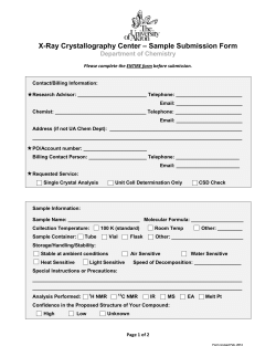


© Copyright 2026