
THE ESP-r COOKBOOK (한국어번역판)
THE ESP-r COOKBOOK (한국어번역판)
Strategies for Deploying Virtual Representations
of the Build Environment
– Ver. 1.0 –
May 1, 2009
Written by
Jon William Hand B.Sc.,M.Arch.,PhD
Energy Systems Research Unit
Department of Mechanical Engineering
University of Strathclyde, Glasgow, UK.
Translated by
Architectural Environmental Planning and Research Center
Department of Architecture
Seoul National University, Seoul, Korea
(역: 서울대학교 건축학과 건축환경계획연구센터)
II
COPYRIGHT DECLARATION
The copyright of this publication belongs to the author under the terms of the
United Kingdom Copyright Acts as qualified by the University of Strathclyde
Regulation 3.49. Due acknowledgement must always be made of the use of any
material contained in, or derived from, this publication.
이 책은 Jon William Hand 박사의 허가에 의해 번역한 것이므로 이 책의 일부
혹은 전체 내용을 무단 복사, 복제, 전재하는 것을 일절 금합니다.
III
IV
NOTICE
If you have any questions or comments on ESP-r COOKBOOK (한국어번역판),
please feel free to contact us through AEPRC (Architectural Environmental
Planning and Research Center) homepage (http://home.snu.ac.kr) or e-mail
([email protected])
ESP-r COOKBOOK (한국어번역판)에 대한 질의사항이나 의견이 있으시면, AEPRC
(건축환경계획연구센터) 홈페이지 (http://home.snu.ac.kr) 또는 이메일 ([email protected])을
통해 연락 주시기 바랍니다.
Kwang Woo Kim, Arch.D.
Professor, Seoul National University
e-mail: [email protected]
김 광 우
서울대학교 건축학과 교수
V
VI
TABLE OF CONTENTS
Abstract .................................................................................................................................. IX
Acknowledgments ................................................................................................................ XI
Translation commitee ........................................................................................................ XIII
1 Introduction ............................................................................................................................. 1
1.1 Tactical approaches .......................................................................................................... 7
1.2 The client specification ................................................................................................ 10
1.3 Design questions .......................................................................................................... 17
1.4 Model planning ............................................................................................................ 21
1.5 Model coordinates ........................................................................................................ 22
1.6 How the building is used .............................................................................................. 32
1.7 Environmental controls ................................................................................................ 37
1.8 Model composition ....................................................................................................... 47
2 Building a model ................................................................................................................. 49
2.1 Review of climate patterns and databases .................................................................... 54
2.2 Locating constructions for our model .......................................................................... 64
2.3 Zone comosition tactics ................................................................................................ 67
2.4 Model topology ............................................................................................................ 97
3 Geometry alternative inputs .............................................................................................. 100
3.1 To the keyboard .......................................................................................................... 103
3.2 Clicking on a bitmap .................................................................................................. 112
3.3 Examples of approaches to take ................................................................................. 115
4 3D Modelling .................................................................................................................... 119
4.1 Modelling approaches ................................................................................................ 121
4.2 Steps to create a roof space ........................................................................................ 129
4.3 Shading obstructions .................................................................................................. 139
5 Schedules .......................................................................................................................... 140
5.1 Scheduled air flows .................................................................................................... 147
5.2 Importing operation schedules ................................................................................... 149
6 Climate data ...................................................................................................................... 151
6.1 Importing climate data ............................................................................................... 152
6.2 Defining seasons and typical periods ......................................................................... 155
6.3 Climatelist entries ....................................................................................................... 161
VII
7 Zone control ...................................................................................................................... 163
7.1 Introduction ................................................................................................................ 163
7.2 Abstract representations ............................................................................................... 166
7.3 Zone control laws ....................................................................................................... 173
7.4 Exploring building control issues ............................................................................... 179
7.5 Controls implementing boundary zones ..................................................................... 198
8 Flow networks ................................................................................................................... 212
8.1 Limitations of Scheduled Flow .................................................................................. 213
8.2 Fluid Flow Networks .................................................................................................. 213
8.3 Building blocks .......................................................................................................... 218
8.4 Steps in creating a network ........................................................................................ 230
8.5 A simple network ....................................................................................................... 234
8.6 To the keyboard .......................................................................................................... 242
8.7 Calibrating flow models ............................................................................................. 248
8.8 Flow control ............................................................................................................... 253
8.9 To the keyboard .......................................................................................................... 259
8.10 Window representations ........................................................................................... 263
8.11 Schedules vs networks ............................................................................................. 269
8.12 Limitation of Network flow ..................................................................................... 278
9 Plant .................................................................................................................................. 280
9.1 First exercise using a component network to represent mechanical
ventilation ......................................................................................................................... 283
9.2 Defining containments ............................................................................................... 292
9.3 Finishing off the model and testing ............................................................................ 293
9.4 Moving from ideal demands to thermal zone demands ............................................. 298
9.5 Links to zones and controls ........................................................................................ 304
10 Install Appendix .............................................................................................................. 312
11 Version Appendix ........................................................................................................... 329
11.1 Text mode ................................................................................................................. 330
11.2 Legacy X11 graphics ................................................................................................ 335
11.3 GT7+ graphics .......................................................................................................... 339
12 ESP-r capabilities ............................................................................................................ 342
Terminology ......................................................................................................................... 373
VIII
ABSTRACT
This Cookbook uses the general purpose simulation suite ESP-r as a platform
to explore strategies for deploying virtual representations of the built
environment to answer questions posed in the real world of design and research
groups.
The Cookbook talks about translating client questions into virtual
representations that are no more and no less complex than is required for the
task. It talks about rediscovering the power of pencils and paper and it dares to
mention the word methodology. And discovering valuable patterns in the clutter
and then learning the art of responding to what if questions. And since the
author is professionally paranoid you might pick up some new definitions of the
word QA.
Almost all of the strategies presented can be applied to the task of creating
elegant virtual representations in other simulation suites. Readers might allert
their colleagues to take a peak.
본 Cookbook은 실제 설계팀이나 연구팀에 부여되는 문제들을 해결하기 위하
여 실제 건물 환경을 가상으로 모사하고자 할 때, 그 전략들을 연구할 수 있는
플랫폼으로서 활용할 일반적인 목적의 시뮬레이션 도구인 ESP-r에 대하여 다루고
있다.
Cookbook에서는 클라이언트의 요구를 적정한 수준의 가상의 표현들로 전환하
는 방법을 기술한다. 또한 이 책은 연필과 종이를 사용하는 기록의 필요성을 강
조하고 있으며 단어 중심의 교수법이라고 할 수도 있겠다. 또한 Cookbook은 무
질서 속에서 가치있는 패턴들을 발견하고 의문에 응답하는 기술을 배우는 것을
다룬다. 독자들은 QA라는 용어에 대한 새로운 정의를 알 수 있을 것이다.
수록되어 있는 거의 모든 전략들은 다른 시뮬레이션 도구에서 가상 모사를 훌
륭하게 하고자 할 때도 활용될 수 있다. Cookbook의 독자들은 (역자 주: 놀라운
지식수준의 향상으로 인해) 치열한 경쟁 속에 있는 동료들을 깜짝 놀라게 할지도
모른다.
IX
X
ACKNOWLEDGMENTS
This Korean translation would not have been possible without my extended
interactions with students and professors in the Department of Architecture of
Seoul National University. In particular I would like to thank Professor Kwang
Woo Kim and Associate Professor Myoung Souk Yeo for the environment of
scholarship, curiosity and hands-on research that I found at SNU. The students
not only acted as subjects for exploring how the skills of creating and using
virtual test environments can be communicated, but also contributed directly
and indirectly to the translation effort.
이 한국번역판은 서울대학교 건축학과의 학생 및 교수님들과의 교류협력이 있었기에
가능하였다. 특히 서울대학교에서의 학문, 탐구, 그리고 실천적인 연구가 가능한 환경을
제공하여주신 서울대학교 김광우 교수님과 여명석 교수님께 감사의 말씀을 전하고 싶다.
서울대학교의 학생들 또한 가상 시뮬레이션을 새롭게 작성하고 이용하는 기술이 어떻게
상호 이해될 수 있는지 탐구하였으며 이 번역작업에 직간접적으로 기여하였음을 밝히고
자 한다.
Jon William Hand
최근 친환경에 관한 관심이 높아지면서 건축물의 에너지 환경성능을 정밀히 예측 시
뮬레이션 하고자 하는 요구가 점점 많아지고 있다. 이에 국내의 건축환경설비 분야에 종
사하는 연구자, 교수, 컨설턴트, 학생들의 효율적인 건물환경 시뮬레이션 기법 습득에 도
움이 되기를 바라는 뜻에서 ESP-r Cookbook 한국어번역판을 준비하였다. 번역을 하는
과정에서 수 차례의 수정을 거치면서 최대한 원본의 내용에 충실하고자 하였지만, 잘못
된 부분이 많으리라 생각된다. 이 책을 참고하면서 내용 중 잘못된 곳을 발견하시면, 언
제든지 지적하여 주시길 바라며, 지적된 사항을 반영하여 빠른 시간 내에 교정본을 낼
것을 약속 드린다.
이번 초판의 발간은 번역과 교정에 참여하신 여러 학생들과 교수님들의 노력이 있었
기에 가능하였다. 특히 이 책을 함께 기획하고 번역작업 중 지속적으로 관심을 기울여주
신 Jon William Hand 박사님께 특별한 감사의 말씀을 전하고 싶다.
김 광 우
Kwang Woo Kim
[email protected]
XI
XII
TRANSLATION COMMITEE
Supervised by
김광우, 건축학 박사
Kwang Woo Kim, Arch.D.
서울대학교 건축학과, 교수
Professor, Seoul National University
Translated by
박사과정
Ph.D. Student
석사과정
M.S. Student
이진영
Jin Young Lee
정창호
Chang Ho Jeong
류성룡
Seong Ryong Ryu
양경운
Kyoung Woon Yang
최동희
Dong Hee Choi
구혜연
Hye Yeon Ku
이선우
Sun Woo Lee
조구상
Goo Sang Joe
구소영
So Young Koo
김희강
Hee Gang Kim
이규남
Kyu Nam Rhee
백승효
Seung Hyo Baek
강동화
Dong Hwa Kang
모백현
Baek Hyoun Mo
조가영
Ga Young Cho
신대욱
Dae Uk Shin
신미수
Mi Soo Shin
이현정
Hyun Jung Lee
김지혜
Ji Hye Kim
홍지표
Ji Pyo Hong
이순명
Soon Myung Lee
김희강
Hee Gang Kim
김일민
Il Min Kim
Reviewed by
최정민, 공학박사
Jeong Min Choi, Ph.D.
창원대학교 건축공학과, 교수
Professor, Changwon National University
김용인, 공학박사, 기계설비기술사
Yong In Kim, Ph.D. / P.E.
나우설비기술(주), 대표이사
President, NOW Consulting Engineers Co., Ltd.
양인호, 공학 박사
In Ho Yang, Ph.D.
동국대학교 건축공학과, 교수
Professor, Dongguk University
석호태, 공학박사
Ho Tae Seok, Ph.D.
영남대학교 건축학부, 교수
Professor, Yeungnam University
XIII
송승영, 공학박사
Seung-Yeong Song, Ph.D.
이화여대 건축학부, 교수
Professor, Ewha University
여명석, 공학박사
Myoung Souk Yeo, Ph.D.
서울대학교 건축학과, 부교수
Associated Professor, Seoul National University
김용이, 공학박사
Yong-Yee Kim, Ph.D.
군산대학교 건축공학과, 교수
Professor, Kunsan National University
박철수, 공학박사
Cheol-Soo Park, Ph.D.
성균관대학교 건축공학과, 조교수
Assistant Professor, SungKyunKwan University
김영돈, 공학박사
Young Don Kim, Ph.D.
㈜하나기연, 소장
Chief of Division, Hana Consulting Engineers Co., Ltd.
조재훈, 공학박사
Jae Hun Jo, Ph.D.
충북대학교 건축공학과, 조교수
Assistant Professor, Chungbuk National University
임재한, 공학박사
Jae Han Lim, Ph.D.
청주대학교 건축공학과, 전임강사
Full-time Lecturer, Cheongju University
김선숙, 공학박사
Sun Sook Kim, Ph.D.
한국건설기술연구원, 선임연구원
Senior Researcher, Korea Institute of Construction
Technology
김지현, 공학박사
Jihyun Kim, Ph.D.
(주)대우건설 기술연구원 건축연구팀,
Researcher, Daewoo E&C Co., Ltd., Korea
선임연구원
XIV
Chapter 1
INTRODUCTION
1 Introduction
Learning how to use simulation tools for design decision support and for research has tended to
follow three paths - the mentor path, the workshop path and the there-be-dragons path. The
mentor path works exceedingly well and is an efficient, if not particularly inexpensive way of
gaining the skills and tactics needed to apply simulation to real-time projects.
건물의 설계 관련 의사 결정 및 연구를 목적으로 시뮬레이션 툴의 사용법을 배우는 것은 세 가지
방법에 의해 이루어질 수 있다. – 지도자 방법, 워크샵 방법, there-be dragons 방법. 진행 중인 프
로젝트에 시뮬레이션을 적용하기 위해 필요한 기술이나 전략을 습득할 만한 특별한 방법이 없다
면 ‘지도자 방법’을 따르는 것이 가장 효과적이다.
Workshops are another successful approach to simulation training. Two or three days of initial
sessions, supplemented by advanced topic workshops and the occasional email allows many
practitioners to productively use simulation. Both of these approaches rely on personal contact
with an expert and iterations of demonstration, followed hands-on experience and dialog for skills
acquisition.
워크샵은 시뮬레이션을 익힐 수 있는 또 하나의 훌륭한 방법이다. 처음 2~3일 간의 워크샵 동안
수준 높은 주제의 강의를 병행하고 이메일을 교환하다 보면, 많은 실무자들이 시뮬레이션을 효과
적으로 이용할 수 있게 된다. 이와 같은 두 가지 방법(‘지도자 방법’과 워크샵)에 있어서 시뮬레이
션 전문가와의 개인적인 접촉, 예제의 반복, 직접적인 체험 및 기술 습득을 위한 대화는 필수적이
다.
Many practitioners rely on mentoring and workshops to keep them up to date as tools evolve and
for exploring new facilities. Documentation tends to lag the evolution of simulation tools and
many lesser-used tasks may not be well documented or documented in ways accessible only to
geeks.
-1-
많은 실무자들이 시뮬레이션 툴의 발전에 발맞추고 새로운 기능을 탐색하기 위해 지도자 방법과
워크샵 방법에 의존한다. 문서화 작업은 시뮬레이션 툴의 발전을 지연시키는 경향이 있고, 자주
이용되지 않는 많은 기능(task)들이 적절히 설명되지 못하거나, 시뮬레이션에 능통한 사람들만 알
수 있도록 설명될 가능성도 있다.
What you are reading now (and the companion Cookbook Exercises is addressed primarily at
those who are taking the path of confronting the dragons. It has also been used to support
workshops in conjunction with the exercise volume.
본 서와 자매서 Cookbook Exercises는 우선적으로 there-be dragons 방법을 선택한 사람들을 대
상으로 기술되었다. 또한 본서는 Cookbook Exercise와 함께 워크샵에서도 사용되고 있다.
The Cookbook strives to be generic in its discussion. As the title suggests, where specific
examples are needed they are based on the ESP-r suite. Some blocks of text apply only to ESP-r
and occasionally you may notice the following icon...
Cookbook에서는 포괄적인 내용을 다루고자 한다. 제목이 암시하는 것과 같이, 특별한 예가 필요
한 경우에 제시되는 예시들은 ESP-r suite를 기반으로 한다. 본문 중 일부 내용은 ESP-r에만 적용
되는 것으로, 다음 아이콘으로 표시된 부분이 이에 해당된다.
If you are reading this from the point of view of another application skip down a few paragraphs.
The Cookbook also includes sections of interest to technical support staff and uber-geeks. These
are marked with the following icon...
당신이 만약 다른 적용의 관점에서 본 서를 읽고 있다면 몇몇 문단은 건너뛰어도 상관없다. 또한
Cookbook은 기술 지원 담당자나 정말 능통한 사람들이 관심을 가질 만한 내용도 포함하고 있으
며, 이는 다음의 아이콘으로 표시된다.
-2-
If you have downloaded one of the precompiled ESP-r distributions for Linux(most distributions),
Mac OSX, Windows(native GUI), Cygwin (emulation under Windows) from the ESRU web site
<http://www.esru.strath.ac.uk> or acquired the source from the source code control repository via
the
uber-geek
command
(on
one
line):
svn
checkout
https://esp-r.net/espr/esp-
r/branches/development_branch and compiled your own version. Most of the instructions needed
to get a working distribution can be found on the download page. Additional instructions are
included with the source and there are discussion lists that might provide additional clues.
ESRU 웹 사이트<http://www.esru.strath.ac.uk>에서 컴파일된 Linux용 ESP-r(가장 많이 배포), Mac
용 ESP-r, OSX용 ESP-r, Windows(native GUI 버전)용 ESP-r, Cygwin(Windows 체제에서 에뮬레이션)
용 ESP-r을 다운로드 했거나, 능통한 사람을 통해 프로그램을 얻었다면: https://esp-r.net/espr/espr/branches/development_branch와 컴파일된 ESP-r의 버전을 확인하라. 유효한 배포판을 얻기 위
해 필요한 대부분의 지침들은 다운로드 페이지에서 찾을 수 있다. 추가적인 지침들은 프로그램
에 포함되어 있으며, 관련 정보를 추가로 제공해 줄 수 있는 토의 목록도 있다.
And the ESP-r download pages do not really tell you much about what to do once you have ESP-r
on your computer. This statement is probably applicable to most other vendors. Of course there
are web based tutorials and exercises as well as manuals that approach telephone directory
proportions.
그리고 ESP-r 다운로드 페이지는 컴퓨터에 ESP-r을 설치하고 난 이후에 무엇을 해야 하는지에 대
해서는 많은 것을 이야기해주지 않는다. 이것은 아마도 다른 많은 프로그램의 경우에 대해서도
마찬가지일 것이다. 물론 전화번호부 책만큼 두꺼운 사용자 설명서뿐 아니라 웹 기반의 강의와
연습자료가 있는 경우도 있다.
Most vendors went through a phase where they believed that web based tutorials would supplant
mentoring and workshops. From the author’s perspective, web pages work less well than the
mentor/workshop paths. The Cookbook is an attempt to bridge this gap. It evolves, as does ESP-r
itself, from observations of practitioners who are attempting to support real-time design
assessments of real-world issues.
많은 프로그램 공급자들이 웹 기반 강의가 지도자 방법과 워크샵 방법을 보완해 줄 수 있을 것이
-3-
라고 믿었지만, 저자의 견해로는 웹 페이지가 지도자 방법이나 워크샵 방법보다 덜 효과적이다.
Cookbook은 이러한 간격을 연결하고자 하는 시도이다. ESP-r 자체가 그렇듯이, Cookbook은 실제
상황에서의 각종 이슈에 대해 실시간 설계 평가를 지원하고자 하는 실무자들을 관찰하는 것으로
부터 발전되어 오고 있다.
Simulation tools almost always arrive with a range of example models of two broad types abstract models which are composed so as to illustrate semantics and syntax and those models
derived from consulting projects which focus on specific building performance design issues. The
first type is often used by novices to get used to the simulation tool, the second type for those
who are looking for examples of best practice models. Vendors do not always make clear which is
which.
시뮬레이션 툴은 거의 항상 두 가지의 일반적 유형에 대한 예제 모델로 시작한다. – 시뮬레이션
의 문법과 구문을 설명하기 위한 목적으로 구성된 추상적 모델과, 컨설팅 프로젝트를 위해 특정
건물의 설계 이슈에 초점을 맞추어 구성된 모델이 그것이다. 첫 번째 유형은 시뮬레이션 툴에 익
숙해지려고 하는 초심자들이 주로 사용하고, 두 번째 유형은 가장 현실적인 모델의 사례를 찾는
사람들이 이용한다. 프로그램 공급자들은 이와 같은 모델의 성격을 항상 명확하게 구분하지는 않
는다.
Example models contain a wealth of information for those who know what they are looking for,
for those who are persistent or for those who are using them as reference materials within the
context of a workshop or in mentor based training. For these users example models can act as:
• a mechanism for exploring the tool (e.g. where do I find out information about environmental
controls, the composition of walls)
• to explore the sequence of tasks required to run an assessment and recover specific
performance metrics
• to explore incremental changes in the description of the model and the performance
implications of such changes
예제 모델은 자신들이 무엇을 찾는지 알고 있는 사람들, 끈기 있게 찾아보는 사람들, 워크샵이나
훈련을 위한 참고 자료로서 모델을 사용하는 사람들에게 많은 정보를 제공한다. 이런 사용자들에
게 예제 모델은 다음과 같은 역할을 할 수 있다.
-4-
• 시뮬레이션 툴을 탐색하기 위한 도구(예. 환경 조절에 대한 정보 또는 벽체의 구성은 어디서 찾
아야 하나?)
• 평가 수행에 필요한 과업의 순서를 탐구하고 특별한 성능 평가요소를 찾아내는 것
• 모델의 정보가 부분적으로 변할 때 이것이 성능 변화에 미치는 영향을 탐구하는 것
Creating a model from scratch under close supervision and with commentary on the approach
taken does reduce the frequency of encounters-with-dragons. In ESRU workshops almost all
participants first model works correctly the first time it is simulated.
새로 모델을 만들 때, 면밀하게 검토하고 자기가 취한 방법에 대해 주석을 달아두면 용과 마주치
는(즉, 난감한 상황) 빈도를 줄일 수 있다. ESRU 워크샵에서는 (이런 점에 유의하여 작업을 하므로)
거의 모든 참가자들의 첫 모델이 처음의 시뮬레이션에서 정확하게 실행된다.
What you are currently reading expands on existing workshop materials and years of mentoring,
recast for the resolution of the printed page.
당신이 현재 읽고 있는 이 Cookbook은 기존의 워크샵 자료와 수년 동안의 교육 자료를 바탕으
로 하고 있으며, 인쇄물의 해상도를 고려하여 재발간된 것이다.
The goal is not simply to act as a dictionary or reference but as a guide to how to approach
realistic design decision support in real time, delivering real information and still have time for a
cup of coffee at the end of the day.
Cookbook의 목적은 단순히 사전이나 참고자료로 사용되는 것이 아니라, 지금 진행중인 건축 설
계에서 의사 결정에 도움을 줄 수 있는 방법을 시뮬레이션을 통해 어떻게 터득할 것인지에 대해
지침을 제공하는 것이다. 또한 실제적인 정보를 제공하면서도 하루를 마감할 때 한 잔의 커피를
마실 수 있는 시간을 갖도록 하는 것이다. (즉 프로젝트에 소요되는 시간을 단축시켜 준다는 것)
This document is based on the premises that readers will already have an intuition about the
physics of buildings and environmental systems. A future revision is planned for those who are
less opinionated. And for readers who are users of other tools there will be much of value even if
the details of implementing the methods differs. Who knows, someday there may be an
-5-
EnergyPlus Cookbook and an EE4 Cookbook.
본 서는 독자가 이미 건물의 물리적 현상과 환경적 시스템에 대해 직관을 갖고 있을 것이라는 전
제 하에 작성되었으며, 향후 발간될 개정판은 배경 지식이 부족한 사람들을 고려하여 작성될 예
정이다. 또한 구체적인 실행 방법은 다르다 하더라도 다른 툴을 사용하는 독자들에게도 매우 유
용할 것이다. 언젠가 EnergyPlus Cookbook과 EE4 Cookbook이 있게 될 지 누가 알겠는가?
A word about ESP-r versions
ESP-r is under active development. On any given day there may be a half dozen commits of code
or documentation or updates to exemplar models to the repository. This Cookbook evolves at a
slower pace. This 2008 version has been revised to match the evolved interface of ESP-r but that
match is likely to be imperfect. Interface entities and paths such as Model Management ->
browse/edit/simulate -> composition -> geometry & attribution may have a different syntax. If
you don’t find a match, please look around for something similar.
ESP-r의 버전 관련 내용
ESP-r은 활발히 발전되고 있는 중이다. 어떤 날이라도 코드, 문서, 예제 모델의 업데이트 등이 여
섯개씩 제작되어 저장소(repository)로 옮겨질 수도 있다. 이 Cookbook은 이보다는 더 느린 속도
로 발전한다. 이 2008년판은 ESP-r의 향상된 인터페이스와 일치시키기 위해 개정되었으나 완전하
게
일치하는
것은
아니다.
인터페이스
개체(entities)
및
Model
Management
->
browse/edit/simulate -> composition -> geometry & attribution와 같은 경로는 다른 방식으로 표
현될 수도 있다. 일치하지 않는 사항을 발견할 경우, 비슷한 다른 것을 찾아보기 바란다.
You may also notice is that some interface related figures in the Cookbook look different from
what you see on the monitor. There are currently three different interfaces for ESP-r. There is the
traditional X11 interface which has its roots in the world of UNIX and Linux. There is an almost
complete port of ESP-r to a graphic library called GT7. GT7 is implemented on a dozen operating
systems and this allows ESPr to be run as a native Windows executable. It also has a more familiar
look and feel and once the port is complete it will be the primary interfaces to ESP-r. The third
interface is a pure-text interface which tends to be used for scripted production work or to enable
ESP-r to act as a background engine for other software. Look in the Version Appendix to see
typical dialogues from the different interfaces.
-6-
또한 Cookbook에 있는 그림과 관련된 일부 인터페이스가 모니터에 보이는 것과 다른 것을 발견
할 수도 있다. 현재 ESP-r에는 세 개의 서로 다른 인터페이스가 있다. UNIX와 Linux 체제에 그 근
원을 두고 있는 전통적인 X11 인터페이스가 있고, ESP-r의 거의 완벽한 체계인 GT7이라 불리는
그래픽 라이브러리가 있다. GT7은 수많은 운영 시스템에서 실행되며 이는 ESP-r이 native
Windows에서 실행될 수 있도록 해 준다. 이것은 또한 좀 더 친숙한 형태와 느낌을 가지고 있으
며 체계가 완성되면 ESP-r의 주된 인터페이스가 될 것이다. 세 번째 인터페이스는 스크립트로 작
성하는 작업에 사용하거나 ESP-r이 다른 소프트웨어의 배경 엔진으로 사용되는 방식에 적용 가능
한 순수한 텍스트 기반의 인터페이스이다. 서로 다른 인터페이스에서 사용되는 전형적인 구문을
보려면 Version Appendix를 참조하라.
With the exception of file browsing facilities, the command sequence needed to undertake most
tasks is almost identical across each of the interfaces. Where facilities differ you may see one of
the following icons followed by specific instructions...
파일 검색 기능을 제외하고, 대부분의 작업을 시작하기 위해 필요한 명령 순서는 각각의 인터페
이스마다 거의 동일하다. 운영체제에 따라 기능이 다른 경우는 다음과 같은 아이콘 중 하나를 볼
수 있는데 이 아이콘을 선택하면 관련정보를 볼 수 있다.
1.1 Tactical approaches
Depending on your personal preferences, getting acquainted with a simulation tool either begins
with exploring existing models (in ESP-r these are called exemplars) or in the context of creating a
model from scratch.
개인적 선호도에 따라 다르겠지만, 시뮬레이션 툴에 익숙해 지는 것은 기존에 작성되어 있는 모
델을 탐구하는 것에서 시작(ESP-r에서 exemplars라 불린다)하거나 모델을 처음부터 새롭게 만드는
것에서 시작한다.
If you are taking the from scratch route grab a note-pad and some sketch paper. The following
-7-
sections explore how you can use ESP-r to arrive at a working simulation model and a growing
set of simulation skills. If you are using a different simulation suite keep reading. Tactics can
almost always be applied universally.
만약 처음부터 새로 만드는 것을 선택하였다면 공책이나 스케치할 수 있는 종이를 준비하라. 다
음 절에서는 시뮬레이션 모델을 만들기 위한 ESP-r의 사용법과 좀더 많은 시뮬레이션 기술에 대
해 탐구할 것이다. 만약 다른 시뮬레이션 도구를 이용하고 있다고 하더라도, 계속 읽어보기 바란
다. 시뮬레이션 툴은 다르더라도, 여기에서 설명되는 전략은 거의 항상 일반적으로 통용되는 것이
기 때문이다.
Let’s begin by deciding what kind of model we are going to make and then plan the work so that
it fits our resources. This is a tactical approach to simulation which concentrates on the art of
making concise models to answer our clients questions without delaying the design process.
먼저 어떤 종류의 모델을 만들 것인지를 결정하고, 다음으로 그 모델이 우리의 역량에 맞게끔 작
업을 계획하자. 이것은 설계 절차를 지연시키지 않으면서도 의뢰인의 질문에 답해 줄 수 있도록,
간결한 모델을 만드는 것에 집중하는 전략적 시뮬레이션 방법이다.
The first table is a powerful dragon slayer. Clients ask us questions – but what are the questions
we ask ourselves as we plan and then compose our virtual worlds?
다음 Table 1.1은 난관을 경감시켜주는 강력한 도구(dragon slayer: 즉 시뮬레이션을 용이하게 해
주는 강력한 도구)이다. 의뢰인들은 우리에게 질문한다. 그러나 우리가 계획하고 실제 세계를 모
델링하면서 우리 자신에게 하는 질문은 무엇인가?
Table 1.1 Initial tactics:
Design Question
Simulation Questions
What do we want to
What thermo-physical issues should be addressed by the model?
know about the design?
How do I know if the
What performance can I measure to inform my judgments?
design works?
What level of model detail is required for this?
-8-
How might the design
What boundary conditions and operating regimes would be a
fail?
reasonable test?
How do I match the
What is the essence of the design in terms of form, composition,
information I have with
operation and control?
the requirements of the
What essential interactions need to be represented?
tool?
What facilities can be employed and what skills are needed to
use them?
Is our approach ok?
Can I sketch out my model and explain it to others?
Are
What assessments need to be undertaken to gain confidence in
the
performance
predictions credible?
the model?
What is expected of a best practice design?
How can I deliver the
What else would clarify how the design works?
most
How might the design and the model evolve during the design
value
for
my
client?
process?
What would I do now to make it easier to work with this model
again after a four month delay?
Table 1.1 Initial tactics
Design Question
설계에 관해 알고 싶어
Simulation Questions
모델에 의해 어떤 열-물리학적 이슈들이 언급되는가?
하는 것은 무엇인가?
설계가 제대로 되었는지
내 판단의 근거를 알리기 위해 어떤 성능을 측정할 수 있는가?
어떻게 아는가?
이것을 위해 어느 정도 수준의 구체화가 필요한가?
어떻게 설계가 실패하는
합리적인 평가를 위해서 어떤 경계 조건과 운전 방법을 적용할
가?
것인가?
내가 가진 정보와 시뮬
형태, 구성, 운전, 제어의 측면에서 설계의 필수 요소는 무엇인가?
레이션 툴에 필요한 조
표현되어야 하는 필수적인 상호작용은 어떤 것이 있는가?
건을 어떻게 부합시키는
어떤 기능(facility)들이 활용되어야 하며 그 기능들을 이용하기 위
가?
해 필요한 기술은 어떤 것이 있는가?
우리의 접근 방법이 적
내 모델을 그려내거나 다른 사람에게 그것을 설명할 수 있는가?
절한가?
-9-
성능 예측은 신뢰할 만
모델의 신뢰성을 확보하기 위해 어떤 평가를 수행해야 하는가?
한가?
어떤 것이 최선의 현실적 설계라고 기대되는가?
의뢰인에게 어떻게 최대
설계가 적절하다는 것을 무엇으로 명확하게 설명할 것인가?
한의 가치를 전달할 것
설계가 진행되는 중에 설계와 모델이 어떻게 발전될 것인가?
인가?
4개월이 지난 후에 다시 이 모델로 작업한다고 하면, 그 작업을
더 쉽게 하기 위해서 지금 나는 무엇을 할 것인가?
Without tactics we will miss out on the value-added aspects of simulation which cost us little to
implement but deliver substantial benefits. A tactical approach keeps you in charge of the
simulation tool.
이와 같은 전략이 없다면, 실행 비용은 거의 들지 않지만 상당한 이익을 줄 수 있는 시뮬레이션
의 부가가치를 놓치게 될 것이다. 전략적인 접근법을 택한다면 당신은 시뮬레이션 툴을 주도적으
로 사용할 수 있게 될 것이다.
Simulation models have a context within which they are created and evolve. In the next section
the clients specification and design questions form the context. From this we decide what type of
model(s) the specification implies as well as the assessment(s) that need to be done to answer the
clients questions or further our research goals. The plural is intentional – real projects are iterative
and models either evolve or spawn the next generations of model.
시뮬레이션 모델들은 일정한 상황 하에서 만들어지고 발전된다. 다음 절에서는 의뢰인들의 설계
명세서나 질문들에 의해 이러한 환경이 형성되는 것을 보게 될 것이다. 이를 바탕으로 우리는 의
뢰인의 질문이나 더 나아가 우리의 연구 목표에 답하기 위해 어떠한 평가를 해야 하는지 뿐만 아
니라, 설계 명세서가 의미하는 것이 어떠한 유형의 모델인지를 결정하게 될 것이다. 실제 프로젝
트는 계속 반복되므로, 모델 또한 지속적으로 진화하고 발전되어야 한다.
1.2 The client specification
The following section provides the specification of our first project. It is designed to allow an
exploration of the best-practice choices made while planning simulation projects.
본 절에서는 우리의 첫 번째 프로젝트에 대한 세부사항에 대해 설명할 것이다. 본 절은 시뮬레이
션 프로젝트를 계획하면서 연습하기에 가장 좋은 대안들을 찾을 수 있도록 구성되었다.
- 10 -
No matter what simulation tool you are using, there is always more than one approach to a
given task. Workshops typically use sequences that are known to work. Mentors will
encourage you to explore alternative approaches. Enlightened managers allocate time for
such explorations.
어떤 시뮬레이션 툴을 사용하더라도, 주어진 과업에 대해 항상 하나 이상의 접근 방법이 있
다. 워크샵에서는 보통 잘 실행된다고 알려져 있는 절차들을 이용한다. 지도자들은 당신이
그 밖의 여러 대안들을 찾아 보도록 장려할 것이다. 의식있는 관리자들이라면 이러한 대안
탐색을 위한 시간을 할애해 줄 것이다.
This initial simulation project is part of a general practitioner’s office. The client specification is
intentionally terse so as to demonstrate typical decisions made by simulation teams in practice.
Clients have beliefs about how buildings work and simulation is one approach which can be used
to confirm or refute such beliefs.
첫 번째 시뮬레이션 프로젝트는 일반 개업의의 병원 일부를 대상으로 한다. 실무에서 시뮬레이션
팀이 내리는 전형적인 의사결정에 대한 예시를 보여주기 위해 의뢰인의 설계 명세는 의도적으로
간결하게 하였다. 의뢰인들은 건물이 어떻게 거동하는가에 대한 믿음이 있고, 시뮬레이션은 그러
한 믿음에 확증을 주거나 또는 반박하기 위해 사용될 수 있는 방법 중의 하나이다.
Figure 1.1 shows a plan and section (looking from the east) of the general practitioner’s office.
The reception has a flat roof and the examination room has a sloped roof with a skylight to the
north.
Figure 1.1은 일반 개업의의 병원 평면과 단면(동쪽으로부터 본 것)을 나타낸다. 접수실은 평지붕
으로 처리되어 있고, 진찰실은 북쪽으로 채광창이 있는 경사지붕으로 되어있다.
- 11 -
Figure 1.1 Plan and section of general practitioner office.
Figure 1.2 is a wireframe perspective view (looking from the south-west). Note the strip windows
on the north of the reception and the two strip windows on the south facade.
Figure 1.2는 와이어프레임으로 표현한 투시도(남서쪽에서 본 것)이다. 접수실 북쪽의 띠창과 남측
입면에 있는 두 개의 띠창을 주목해라.
- 12 -
Figure 1.2 Wire-frame view of general practitioner office.
Figure 1.3 is a colour rendering (looking from the south-west) which was created by exporting the
ESP-r model to Radiance.
Figure 1.3은 ESP-r 모델을 Radiance로 export하여 만들어진 컬러 렌더링(남서쪽에서 바라본 것)이
다.
Figure 1.3 South-west view of general practitioner office
- 13 -
Figure 1.4 is a view from the north-west through the examination room. The white surfaces
represent walls which are partitions to a portion of the building which has not been included
within the model.
Figure 1.4는 북서쪽에서 본 진찰실로, 흰 색 표면은 모델에 포함되지 않은 건물 일부분에 면한
간막이벽을 나타낸다.
Figure 1.4 North-west view of general practitioner office.
This project represents a portion of a general practitioner’s office. Focusing initially on a
portion of a building is a powerful strategy and one which is applicable to almost all
simulation tools.
이 프로젝트는 일반 개업의의 병원 일부를 표현하고 있다. 초기에 건물의 일부분에만 초점
을 맞추는 것은 문제해결을 위한 강력한 전략이고 이는 거의 모든 시뮬레이션 툴에 적용
가능한 것이다.
- 14 -
The client indicates that this medical practice has a brisk turn-over of clients and that, on average,
there are two people in the examination room during the hours of 9h00 to 16h00 on weekdays
(200W sensible, 100W latent). The reception area serves other portions of the building which are
not included in this model and there might be up to five people. Lighting in the reception is
150W during the hours of 8h00 to 19h00 and there are no small power loads in either room for
purposes of this model.
의뢰인에 의하면 병원에는 많은 환자들이 찾아오며, 주중에는 9시부터 16시까지 진료실에 평균적
으로 2명이 있다고 한다(현열 200W, 잠열 100W). 접수 공간은 이 모델에 포함되지 않은 병원의
다른 부분을 위한 공간이며, 사람이 5명 까지 있을 수도 있다. 접수실의 조명은 8시부터 19시까
지 150W이며, 이 모델의 두 실에 기타 전열 부하는 없다.
The heating set point is 20°C and the cooling set point is 23°C between 9h00 and 17h00 on
weekdays with frost protection (15°C) on weekends. The client has no specific opinion as to how
this is to be achieved.
주중에 9시부터 17시까지의 난방 설정온도는 20℃이고 냉방 설정온도는 23℃이며, 주말에는 동파
방지를 위해 난방온도를 15℃로 설정한다. 의뢰인은 이 설정온도를 달성하는 방법, 즉 냉난방 수
단에 대해서는 특별한 의견을 가지고 있지 않다.
ESP-r, unlike some simulation suites, includes both ‘ideal zone controls’ and component based
descriptions of environmental systems. In this exercise we will start with a minimalist ‘ideal’
description and assume that both heating and cooling are assumed to be delivered convectively.
ESP-r demands an initial guess at the heating and cooling capacity, but otherwise we will maintain
our focus on demand side issues.
다른 시뮬레이션 툴과 달리 ESP-r은 환경 조절 시스템(environmental systems)에 대하여 ‘이상적인
존 컨트롤’ 기능과 실제 설비 시스템 기반의 모델링 기능 두 가지를 모두 제공한다. 이 예제에서
는 이상적인 존 컨트롤이 이루어지는 상황을 먼저 모델링할 것이며, 냉난방 모두가 대류에 의해
이루어진다고 가정할 것이다. ESP-r은 냉난방 용량(capacity)에 대해 초기 가정치를 필요로 하나,
일단 공간의 냉난방 필요량에 초점을 맞추어 진행할 것이다.
- 15 -
Questions to ask about auto-size functions:
a) what boundary condition(s) and operational regime(s) are associated with peak
conditions?
b) what method(s) are used to assess intra-component dependencies as components are
sized?
c) what criteria are used to determine which sub-optimal set of component sizes works
best?
d) what criteria might you use to confirm the suggested sizes?
Auto-size 기능 (설비 시스템의 용량을 자동으로 선정하는 기능)에 대한 질의 사항:
a) 최대부하조건과 관련된 경계조건과 운전 방식은 어떠한 것인가?
b) 설비 시스템의 용량을 산정할 때, 시스템 간의 상호의존성을 평가하기 위해 어떤 방법들
이 사용되는가?
c) 설비 시스템의 용량을 결정하기 위한 대안 중 가장 최적의 조합안을 결정하기 위해서는
어떤 기준들이 사용되는가?
d) 제시된 설비 시스템의 용량을 확정하기 위해 어떤 기준을 사용할 것인가?
Components might seem unambiguous. Be sceptical until you can confirm that they match
your expectations.
선택된 설비 시스템들은 명백히 타당하게 보이겠지만, 그것이 당신이 기대하는 바와 부합한
다는 확신이 들 때 까지 질문에 질문을 거듭하라.
- 16 -
Back to our initial model. Even the best of buildings have infiltration. There is a discussion about
air flows in a later section. For now lets use an initial engineering assumption that there will be
0.5 ac/hr infiltration at all hours.
우리의 첫 번째 모델로 돌아가 보자. 아무리 잘 지어진 건물이라 하더라도 침기가 있다. 나중에
기류에 대해 다루는 부분이 있겠지만, 지금은 우선 공학적인 가정으로서, 매시간 0.5ACH의 침기
가 있다고 가정하자.
1.3 Design questions
The client wants to know what the typical demands for heating, heating capacity, thermal comfort
in the winter and summer, whether it is likely to overheat and if the daylight distribution is ok.
의뢰인은 난방 요구량, 난방 용량, 여름과 겨울의 열쾌적 수준 등에 대한 정보 뿐 아니라 건물이
과열(overheat)되기 쉬운지, 자연채광의 분포가 양호한지 등에 대해서도 알기를 원한다.
To answer these questions we require a model which represents the general form, composition
and use as described in the client specification. The model need not be particularly detailed and
our goal is to maintain the volume of the spaces as well as the orientation, area, distribution of
mass and general shape of the room surfaces.
이러한 질문에 답하기 위해서는 의뢰인의 명세서에 묘사된 것과 같은 일반적인 형태, 구성, 용도
가 표현되어 있는 모델이 필요하다. 이 모델은 특별히 상세하지는 않아도 되며, 향, 면적, 공간의
분포, 실 표면의 일반적인 형태뿐 등을 실제와 유사하게 만드는 것이 가장 중요하다.
Review Table 1.1. If the client asked different questions the nature of the assessments might well
be different.
Table 1.1을 다시 봐라. 의뢰인이 다른 것에 대해 궁금해 시뮬레이션 평가는 당연히 다른 관점에
서 이루어져야 한다.
So, what sort of assessments will address the question of typical heating and cooling demands,
- 17 -
capacity and comfort? If we weren’t thinking tactically we might run an annual simulation and
then get bogged down in scanning the predictions for useful information.
냉난방 요구량, 냉난방 용량, 쾌적에 대한 질문에 답하기 위해서는 어떤 종류의 평가를 해야할 것
인가? 우리가 전략적으로 생각하지 않는다면 필요도 연간 시뮬레이션을 수행하고, 그 결과에서
유용한 정보를 찾으려고 하다가 수렁에 빠져들지도 모른다.
A tactical approach limits the quantity of information we have to deal so both the model
and its performance is easier to understand and the QA burden is reduced. Lets look first
on seasonal patterns to highlight performance issues. Computers may process a year in
seconds but QA staff costs are greater.
전략적 접근은 우리가 다루어야 할 정보의 양을 줄여주므로, 모델(그 자체)과 모델의 성능
모두 이해하기가 한결 쉬워지고 질의/응답에 대한 부담도 감소된다. 모델의 성능에 대한 이
슈를 살펴보고자 할 때에는, 계절별 패턴을 우선적으로 살펴보라. 컴퓨터는 몇 초 만에 1년
치를 처리할 수 있지만, 전략적 접근을 하지 않을 경우 질의/응답에 소요되는 비용이 증가
될 수 있다.
The key initial objective is to support our own understanding of performance by looking at
patterns in a limited set of data and so be able to spot glitches in our model as well as
opportunities for improvements to the design (or the clients specification) as soon as possible.
첫 번째 중요한 목적은 한정된 데이터들의 패턴을 봄으로써 건물의 성능에 대한 우리 스스로의
이해를 돕는 것이다. 또한 그럼으로써 가능한 빨리 설계(또는 의뢰인의 명세서)를 개선할 기회뿐
아니라 모델 자체의 결함을 포착할 수 있도록 하는 것이다.
Value added: The client did not ask for it, but it takes little extra effort to check for typical spring
- 18 -
and autumn performance might provide useful feedback to the design team.
부가 가치: 봄과 가을의 건물 성능을 확인해 보는 것은 의뢰인이 별도로 요청한 사항이 아니더라
도 추가적인 노력은 거의 들이지 않으면서 설계팀에게 유용한 피드백을 제공해 줄 수 있다.
Another tactic is to define performance metrics (e.g. what can we measure in our virtual world)
early in the process. Some metrics e.g an energy balance within a zone, might contribute to our
own understanding of the design and other metrics e.g. thermal comfort might be useful to
report to others in the design team.
또 다른 전략은 성능지표(performance metrics: 예를 들어 우리의 가상 세계에서 측정할 수 있는
것 등)를 초기 단계에서 정의하는 것이다. 예를 들어 존에서의 에너지 밸런스와 같은 일부 지표는
설계에 대한 이해를 도울 수 있고, 열쾌적과 같은 척도는 설계 팀 내의 다른 사람에게 보고하는
데 유용하게 사용될 수 있다.
ESP-r workshops typically devote as much time to exploring building performance issues as is
spent on model creation. Simulation suites which do not include an interactive exploration facility
will include a descriptive language to specify what performance metrics are to be captured during
each assessment - so learn that language!
ESP-r workshop은 모델을 완성하는데 소비되는 시간만큼 건물 성능에 관한 이슈를 탐구하는데
많은 시간을 쏟는다. 쌍방향의 탐색 기능이 포함되지 않은 시뮬레이션 도구들은 시뮬레이션 평가
를 할 때마다 어떤 지표를 찾아보아야 하는지를 설명하기 위한 서술을 포함하게 되므로, 그 서술
을 이해해야 하는 어려움이 따른다.
The metric for heating and cooling demands is kWhr (integrated) over the week and for capacity
the metric is diversified kW (the peak capacity required for this portion of the building). Just to be
sure that the pattern of demand is reasonable we will want to graph this. In addition to a table of
demands and capacity we might include the graph in our report if it proves of interest.
냉난방 요구량을 위한 평가 지표는 주(week) 단위의 통합 kWhr이고, 냉난방 용량을 위한 평가 지
표는 순간적인 kW(건물의 이 부분을 위해 요구되는 최대 용량)이다. 수요 패턴이 합리적이라는
- 19 -
것을 확실히 나타내기 위해서는 그래프로 표현하는 것이 좋다. 이것이 중요하다고 판단된다면,
보고서에 냉난방 필요량과 용량을 나타낸 표 외에 추가로 그래프를 포함시키게 될 것이다.
Resultant temperature is a common comfort metric. A frequency bin of resultant temperatures
during the occupied periods would inform the client about the distribution of comfort. For our
own use, we also want to check the number of hours over 24°C and graph the temperatures, we
might include these in our report if they prove interesting.
합성 온도는 일반적인 쾌적 평가 지표이다. 재실 기간 중 합성 온도의 빈도 분포는 의뢰인에게
쾌적 분포에 대한 정보를 제공해 줄 수 있다. 또한 24°C를 초과하는 총 시간을 확인하고 이 때의
온도를 그래프로 나타내고 싶을 수도 있으며, 그 결과들이 흥미롭다고 판단되면 보고서에 이를
포함시킬 것이다.
To answer the question about daylighting we can look at daylight factors across a grid in each of
the rooms. To build a model that will answer questions of thermal and lighting performance we
need to decide how much geometric resolution if required. In the case of daylight factors the
level of detail needed for the thermal assessment should suffice. If glare was to be assessed the
model would need to include additional visual geometric details. Later on we will consider tactics
that anticipate probable future design performance questions.
QA tip: Write down these decisions, we will want to review them as the project progresses to
make sure we are working to-the-plan.
자연채광과 관련된 질문에 답하기 위해서는 실의 여러 지점에서 주광률을 검토할 수 있다. 열 및
빛 환경 성능 평가를 위한 모델을 구축하기 위해, 필요하다면 얼마나 높은 기하학적 해상도를 적
용해야 할지 결정해야 할 필요가 있다. 주광률의 경우, 온열환경 성능평가를 위해 필요한 정도의
상세 수준이면 충분하다. 만약 현휘를 평가하고자 한다면, 좀 더 상세하게 시각적으로 형상화하여
모델링하여야 한다. 추후에, 설계 안의 성능에 대한 질문들을 미리 예상할 수 있는 전략에 대하여
살펴보게 될 것이다.
QA tip: 이러한 결정을 기록하라. 프로젝트가 진행됨에 따라, 우리가 계획에 맞게 작업하고 있는
지를 확인하기 위해 그 기록들을 살펴보게 될 것이다.
- 20 -
1.4 Model planning
Get out your grid paper and note pads and keep the laptop lid closed for now. Pre-processing
information and sketching the composition of our model will limit errors and make it easier for
others to understand what we intend to create, and, after we have made it, to help check that it is
correct. This rule applies whether we are going to import CAD data or use the in-built CAD
functions of our simulation tool.
모눈이 있는 종이와 공책을 꺼내고 지금부터 노트북 컴퓨터의 뚜껑을 닫아라. 정보를 사전에 정
리하고 모델 구성에 대해 스케치하는 것은 오류를 줄여 주며, 다른 사람들이 우리가 만들려고 하
는 것이 무엇인지 쉽게 이해할 수 있도록 해준다. 또한 모델을 다 만든 후에는 그것이 제대로 되
었는지를 쉽게 확인할 수 있도록 해 준다. 이러한 원리는 CAD 데이터를 들여오거나 혹은 ESP-r에
내재된 CAD 기능을 이용할 때에도 적용된다.
It also saves time and removes another source of error if we convert the important horizontal and
vertical dimensions (such as those shown in Figure 1.1) to model coordinates and include them in
our planning sketches. This avoids jumping between a keyboard and a calculator during model
definition as well as helping in QA tasks
중요한 수평 및 수직의 치수(Figure 1.1에서 보여진 것들과 같은)를 모델 좌표로 변환하고 계획 스
케치에 그것들을 포함한다면 시간을 절약하고 오류의 다른 원인을 제거할 수 있다. 이것은 QA
업무량을 줄여 도움을 줄 뿐 아니라 모델을 구축하는 동안에 키보드와 계산기 사이를 왔다 갔다
하는 것을 방지해준다.
User friendly software does not reduce the need for planning or robust QA. If anything, it is
even more important to guard against needless complexity. Lets call this avoiding the dark
side.
- 21 -
사용자 친화적인 소프트웨어라고 해서 사전 계획이나 힘든 QA 작업의 필요성이 줄어들지
는 않는다. 어떤 것이든지, 불필요하게 복잡해지는 것을 방지하는 것이 훨씬 더 중요하다.
이것을 어두운 면의 회피(avoiding the dark side)라고 부르자.
An exercise related to model planning is included in the Cookbook Exercises within Exercise 1.
모델 계획에 관련된 예제는 Cookbook Exercises의 Exercise 1에 포함되어 있다.
1.5 Model coordinates
Novice practitioners often proceed under the assumption that geometric input consumes the bulk
of their project time. Seasoned simulationists know that geometry takes about a third of their
project time and they evolve strategies to help them limit the time spent on creating and
checking geometric entities (so they will have the time and attention to leverage value added
opportunities that might arise).
업무에 처음으로 입문하는 사람들은 종종 건물의 형태를 모델링하는 작업에 프로젝트 시간을 다
소비해버린다. 경험이 많은 사람들은 형태를 모델링하는 부분에 프로젝트 시간의 3분의 1이 소요
됨을 알고, 개체의 생성과 검증에 소요되는 시간을 줄이는 전략을 사용한다(부가가치의 효력 창출
을 위한 시간과 집중을 위해서).
An experienced user can generate models with scores of thermal zones that fit together correctly
the first time. Such skills can be acquired over time. We are going to walk before we run, and our
initial goal is to create a correct three zone model for the doctors office. In workshops nine out of
ten participants create models which simulate correctly the first time.
숙련된 사용자들은 처음 시도만으로 정확하게 들어맞는 여러 개의 thermal zone을 만들 수 있다.
이러한 기술은 오랜 시간에 걸쳐 습득될 수 있다. 그러나 우리는 달리기 전에 걷는 것이 우선되
- 22 -
어야 하므로, 첫 번째 목표는 병원을 위한 3개의 존 모델을 정확하게 만들어 내는 것으로 설정한
다. 워크숍에서 참가자 10명중 9명은 첫 번째 시도에서 시뮬레이션 모델을 정확하게 만들어 낸다.
If asked, most are able to re-create this model with minimal support and in 25-35% less time. So
even though an experienced user will outpace a novice, good working practices ensure that even
novices can produce useful models. The approach we take to create the form of the model is as
dependant on the questions we wish to address with the model as it is on the specifics of the
building blocks and input facilities that are offered by the simulation suite.
만약에 요청 받는다면, 대부분의 사람들은 최소한의 도움만으로 이 모델을 다시 만들 수 있고, 모
델 작성에 소요되는 시간을 25~30% 줄일 수 있을 것이다. 비록 숙련자가 초보자보다 속도는 빠
르더라도, 연습을 잘 한다면 초보자도 반드시 유용한 모델을 만들 수 있게 된다.
우리가 모델을 만들면서 접근하게 되는 방법은 시뮬레이션 툴이 제공하는 각종 기능에 의해서도
좌우되지만, 스스로 알아보고자 하는 내용에 따라서도 달라지게 된다.
• questions about general comfort and energy demands at peak and moderate climate conditions
require only a moderate geometric resolution e.g. correct volume of the space, approximate
location of doors and windows
● 최대부하조건 및 적당한 기후조건 하에서 일반적인 쾌적 상태와 에너지 요구량에 대해 알기
위해서는 적당한 수준의 기하학적 해상도만 적용해도 된다. 예를 들면 공간의 정확한 부피, 대
략적인 문과 창문의 위치
• questions related to comfort at a specific location require higher geometric resolution, especially
if surface temperatures are likely to be vary across a surface
● 특정 위치에서의 쾌적과 관련된 문제, 특히 어떤 표면에 걸쳐 표면온도가 다양하게 분포한다
면 높은 수준의 기하학적 해상도가 필요하다.
• question related to visual comfort will require higher geometric resolution for facades and may
require that furniture within rooms and outside obstructions be accounted for
- 23 -
● 시각적 쾌적과 관련된 문제에는 건물 외피에 대한 더 높은 수준의 기하학적 해상도가 필요할
것이고, 실내 가구 또는 실외의 장애물을 고려해야 할 수도 있다.
• questions related to the distribution of air temperature within a physical space may require that
it be represented by more than one thermal zone or that it include a CFD domain
● 물리적 공간 내의 실온 분포와 관련된 질문은 하나 이상의 thermal zone으로 표현하거나 CFD
영역에 포함시켜 해석해야 할 수 있다.
• questions related to passive solar performance may require a higher level of geometric and
construction detail to assess the impact of mass and the distribution of solar radiation
● 자연형 태양열 설계(passive solar)의 성능과 관련된 문제에는 높은 수준의 기하학적 해상도가
필요하며, 건물 매스의 영향과 일사의 분포를 평가하기 위해서는 더 자세한 건축 디테일이 요
구될 수 있다.
Each of these issues require that we first consider the physics underpinning the assessment.
Second we must search the available model building blocks for relevant entities. Lastly we must
consider what resolution to apply those entities within our model. For example, a passive solar
design will be sensitive to heat stored in the fabric of the room as well as details of glazing in the
facade and in partitions to adjacent rooms. The surface temperatures in a sun patch might be
substantially elevated.
이러한 각각의 이슈는 평가의 기초가 되는 물리학을 첫 번째로 고려할 것을 요구한다. 두 번째로
관계된 개체를 모델링하기 위해 적합한 건물 관련 블록들을 찾아야 한다. 마지막으로 모델 내에
서 이러한 개체를 반영하기 위해 어느 정도의 해상도를 적용할 지에 대해 생각해야 한다. 예를 들
어, 자연형 태양열 설계(passive solar design)는 인접공간에 면한 간막이벽, 외피의 유리를 구성하
는 디테일 뿐만 아니라 공간을 둘러싼 구조체에 저장되는 열 등에 민감하게 좌우되므로, 모델의
해상도를 높여 해석해야 한다. Sun patch에서의 표면 온도는 큰 폭으로 상승할 것이다.
To find out where the sun falls in the room at different times of the year we might create a rough
model and then check what we can see in a wire-frame view at different times of the year. Our
goal would be to find out if we need to subdivide surfaces to better reflect the temperature
- 24 -
differences in insolated and uninsolated portions. We can then make a variant of the zone with
higher geometric resolution and compare the predicted surface temperatures.
한 해의 다른 여러 시점(時点)에서 방안으로 태양이 비치는 곳을 찾기 위하여 개략적인 모델을 만
들고, 여러 시점에서 와이어프레임 뷰로 무엇을 볼 수 있을지 체크한다. 여기서의 목적은 햇볕이
드는 부분과 그렇지 않은 부분의 온도 차이를 더 잘 반영하기 위하여 표면을 나누는 것이 필요한
지의 여부를 판단하는 것이다. 기하학적인 해상도가 다른 여러 개의 존을 만들어서 표면 온도 예
측 결과를 비교 할 수 있다.
As a general rule the design of models should ensure that the volume of the air is close to the
correct value just as we want to ensure that the surface area is correct and that mass within the
rooms is appropriately distributed. In the doctors office the windows are not large and the
questions are general and so the exact location of the windows is not critical (but it costs us
nothing to place them accurately).
The dimensions shown in Figure 1.1 should be straightforward to represent. Looking closer, there
is no thickness indicated so the criteria used to arrive at the dimensions is unclear. If you were
tasked with determining dimensions from information supplied by a client a set of rules would be
useful.
일반적으로, 모델의 설계에 있어서 실내의 공간들이 적합하게 분포되어 있는지, 표면적과 공간의
체적이 최대한 정확한지 등을 확인해야 한다. 병원 건물에서 창문은 넓지 않고, 모델을 통하여 알
고자 하는 내용은 일반적인 것이므로 창문의 정확한 위치는 중요하지 않다(그러나, 창문을 정확하
게 위치시키더라도 전혀 비용은 들지 않는다.) Figure 1.1의 치수는 직관적으로 표현되어야 한다.
더 자세히 보게 되면, 두께가 표시되지 않았기 때문에, 치수를 표기하는 기준이 불명확하다. 만약
에 의뢰인이 전달해준 정보로부터 치수를 결정하는 업무를 맡았다면, 치수를 표기하는 기준을 이
용하는 편이 유용할 것이다.
• Where the volume of the space is large with respect to the thickness of the facade and where
the complexity of the facade is low it is common to measure from the inside face of exterior
walls.
● 공간의 체적이 외피의 두께에 비해 크고 외피의 복잡도가 낮은 곳에서는 외벽의 내부 표면에
- 25 -
서부터 치수를 재는 것이 일반적이다.
• Measuring partitions at each face is common where the coordinates are taken from CAD
drawings and at the centre line during the sketch stage.
● CAD 도면에서 좌표를 가져오는 경우에는 간막이벽의 양쪽 표면에서부터 치수를 재는 것이 일
반적이며, 스케치 단계에서는 간막이벽의 중심선에서부터 치수를 재는 것이 일반적이다.
• Ceiling voids or raised structural floors with little or no air movement are often represented as
layers of air in constructions.
● 기류가 거의 없거나, 아예 없는 천장 속 공간(Ceiling voids) 또는 뜬 바닥(raised structural
floors)은 구조체 내부의 중공층처럼 모델링한다 (즉 열저항만 부여함).
• Where air movement is likely or there are significant heat gains within the void they may be
better represented as a separate thermal zone.
● 빈 공간 내에 기류가 있거나 열획득량이 상당할 경우에는 별도의 thermal zone으로 모델링하
는 것이 좋다.
• As ceiling (below) to floor (above) distances increase it makes sense to take the height coordinates literally and geometrically separate levels within buildings.
● 아래층의 천장에서부터 위층의 바닥까지의 거리(즉 스팬드럴 높이)가 증가함에 따라, 높이 좌
표를 취하여 건물 안에서 실제로도 구분되고 기하학적으로도 구분된 층을 표시하는 것이 합리
적이다.
• There are ESP-r exemplar models which have the zones on each side of a partition in the same
plane and other exemplars have zones separated in space.
● 간막이벽의 양쪽 면이 각각 다른 존에 면하고 있는 예제 모델이 있고, 한 공간 안에 구분된
존들을 가지고 있는 예제 모델이 있다.
- 26 -
• In most simulation tools it is a matter of personal preference because the heat flow between
zones is established by specific directives partn_cor in office is connected with partn_off in
corridor which are separate from the geometric definition.
● 대부분의 시뮬레이션 툴에서, 간막이벽을 매개로 두 존을 모델링하는 문제는 개인적인 선택의
문제이다. 이는 기하학적 측면에서는 분리되어 있는 partn_off in corridor(‘복도에 있는 사무실의
간막이벽’이라는 의미)간막이벽과 partn_cor in office(‘사무실에 있는 복도의 간막이 벽’이라는 의
미)간막이벽을 연결시키는 특정한 명령어에 의해 존 사이의 열류량이 결정되기 때문이다.
• Most simulation tools represent geometry as polygons and separately represent their
composition.
● 대부분의 시뮬레이션 툴은 다각형으로 기하학적인 모양을 나타내고, 그 구성에 대해서는 별도
로 나타낸다.
• Wire-frame displays often present models as having walls of little or no thickness.
● 와이어 프레임 표현은 벽의 두께가 거의 없거나 두께가 완전히 없는 것으로 모델을 나타낸다.
• For modern (thin) construction the wireframe display may provide an image that allows us to
forget that real walls have thickness.
● 현대적인 (얇은) 구조체에 대하여, 와이어프레임 표현은 우리로 하여금 실제 벽의 두께를 잊도
록 만드는 이미지를 나타내게 될 지 모른다.
• Consider the modern office construction in Figure 1.5 there will be little or no change in
predictions whether the centre line or the actual location in space is used.
● Figure 1.5의 현대적인 사무소 건물의 구조체를 보자. 여기에는 중심선이 사용되었든지 아닌지,
또는 공간 안에서 벽체가 실제 위치에 있든지 없든지 결과에는 별 차이가 없을 것이다.
- 27 -
• Given that there are doors in the partition there is a strong case for adopting the centre line to
avoid visual confusion.
● 간막이벽에 문이 있는 경우, 시각적 혼란을 피하기 위하여 중심선을 적용한 단적인 예가 있다.
Figure 1.5 Plan of a modern building.
At the other extreme, historical buildings can have exterior walls and partitions which vary in
thickness and are substantially different from the thickness of doors. In Figure 1.6 the inside and
outside faces are multi-faceted the shape of the window surround influences the distribution of
light within the room. Some partitions are thin enough to be treated as centre lines and others
suggest a separation of the thermal zones.
이와 다른 극단적인 예를 보면, 역사적인 건물은 문의 두께와는 상당한 차이를 보이는, 다양한 두
께의 외벽과 간막이벽으로 되어있다. Figure 1.6에서 벽면의 안쪽과 바깥쪽 면은 다면체와 같이 각
이 져있으며 창문의 형태는 실내 빛의 분포에 영향을 미치도록 되어있다. 몇몇 간막이벽은 중심
선으로 표현될 만큼 가늘고, 다른 간막이벽들은
별도의 thermal zone을 구획해야 할 만큼 두껍
게 되어있다.
- 28 -
Figure 1.6 Plan of a historic building.
Translating the historical plan into a model required a number of decisions to represent in one
dimensional heat flow paths a building which is a substantially three dimensional heat flow
problem. The result, shown in Figure 1.7, substantially retains the volume and positions of the
spaces rather than the exterior form of the building. Thin partitions are taken to the centre line.
Some plan detail has been omitted and minor spaces amalgamated into adjacent rooms. Having
sketched on an overlay what we wanted to transcribe, the actual creation of the initial extruded
form of the rooms was accomplished in a matter of minutes via a click-on-bitmap facility.
역사적인 건물의 평면(histrocal plan)을 분석하여 모델로 만드는 경우, 본질적으로는 3차원적인 열
류해석의 문제를 일차원 열류로 해석하기 위해 많은 결정이 필요하다. 그 결과는 그림 1.7에서 보
듯이, 겉으로 보이는 건물의 형태 보다는 공간의 부피와 위치가 원래대로 유지되는 가에 달려있
다. 가는 간막이벽은 중심선으로 나타내져 있다. 평면에서 몇 개의 디테일은 생략되었고, 중요치
않은 공간들은 인접 실로 통합되었다. 우리가 옮겨 그리기 원하는 것 위에다 스케치를 한 후,
방
들을 밀려올려진(extruded) 형태로 만드는 것은 click-on-bitmap 기능을 통해 몇 분만에 만들어
낸 것이다
- 29 -
Figure 1.7 Model of a historic building.
The geometry at the window heads and sills was then adapted and the doors inserted. When
attributing the surfaces, the associated construction was selected to account for the local cross
section. A further discussion about options for interpreting complex three dimensional designs
into appropriate models can be found in Chapter 4. The Cookbook is concerned with the art of
composing models which are specifically adapted to the needs of the design process. Not all
projects are as demanding as the historic building. There is also an art to creating models which
are fit for the sort of general questions posed in the doctors office. While planning a model we
might ask ourselves:
창문의 인방과 창문턱의 기하형상은 적절히 변형되었고, 문이 삽입되었다. 표면의 속성을 정의할
때, 해당 구조체의 구성은 프로젝트가 수행되는 지역에서 사용되는 단면구성에 적합하도록 선택
되었다. 복잡한 3차원 설계를 보다 단순한 모델로 해석하기 위한 옵션에 관해서는 4장에 설명되
어 있다. cookbook은 설계 과정에서 특별히 필요로 하는 모델을 만드는 기술에 초점이 맞추어져
있다. 모든 프로젝트가 역사적인 건물의 경우와 같은 큰 노력을 요하지는 않는다. 병원 건물에서
제기되었던 일반적인 질문에 적합한 모델을 만드는 기술 또한 있다. 모델을 계획하는 동안 우리
는 다음을 염두에 두어야 한다.
- 30 -
• would patterns of temperature and heating change if the volume of the space was off by the
width or a wall?
● 만약 폭이나 벽을 조정함으로써 공간의 체적이 없어지면 온도와 난방의 패턴이 변화할 것인
가?
• would more sunlight enter the room if a window was lowered by 5cm?
● 만약의 창문이 5cm 낮아지면 더 많은 빛이 방으로 들어갈 것인가?
• is it necessary to include the frame of the window?
● 창문의 프레임을 포함하는 것이 필요한가?
• is it necessary to include the furniture within the rooms?
● 방안에 가구를 포함하는 것이 필요한가?
Essentially our concern is to ensure that the uncertainty in the model is constrained to the point
where it would be unlikely to change a design decision. Each of the above bullet points could, in
fact, be tested by creating model variants and then looking at the performance differences. There
are many simulation groups who have undertaken such parametric studies to arrive at their rule
set. For this initial exercise the rule is keep it simple. The X axis in ESP-r is towards the East and
the Y axis is towards the North.
모델의 불확실성으로 인해 설계 단계에서 의사 결정이 변화되지 않도록 모델의 불확실성을 축소
시키는 것은 필수적이다. 사실 위에서 불릿으로 구분하여 기록한 각 항목은 적절하게 모델을 만
든 후 변수 값을 다양하게 바꾸면서 성능의 차이를 확인함으로써 테스트될 수 있다. 자신들만의
규칙(rule set)에 도달하기 위해 그러한 변수 연구(parameter study)를 진행해온 많은 시뮬레이션
그룹이 있다. 여기서 하는 첫 번째 연습의 규칙은 “단순하게 하라”이다. ESP-r의 X축은 동쪽방향이
- 31 -
고, Y축은 북쪽 방향이다.
Most users find it convenient to keep their model in positive coordinates and to define their
model using cardinal orientations and later rotate and transform the model to reflect conditions
at the site. Figure 1.8 shows critical coordinates (X,Y) derived from Figure 1.1. To simplify our task
let us assume that the origin of the model is at the lower left corner of the examination room.
The critical vertical points to record on your notepad are 0.0 (ground), 2.0 (window sill), 3.0
(ceiling), 4.5 (top of sloped roof). Taking the time to gather and confirm critical co-ordinates in the
plan and sections before going to the keyboard
is a key technique in getting-it-right the-first-time.
대부분의 사용자는 양의 좌표계에서 모델링 작업을 하고 기본 방위에 맞추어 모델을 만든 다음
나중에 부지의 조건을 반영하기 위하여 모델을 회전하고 변형시키는 것이 편하다고 생각한다. 그
림 1.8은 그림 1.1로부터 정의된 중요한 좌표(x,y)를 보여주고 있다. 과제를 단순화하기 위하여 모
델의 원점이 진료실의 왼쪽 아래 꼭지점에 있는 것으로 가정한다. 컴퓨터 키보드로 가기 전에 시
간을 가지고 평면과 단면의 중요한 좌표를 확인하는 것이 첫번째 단추를 잘 끼우기 위해 중요한
핵심 기술이다.
Figure 1.8 Critical dimensions taken from the plan.
1.6 How the building is used
Our next stage in the planning process is to deal with how the building is used (schedules of
occupants, lighting, small power). The client specification must be transformed into schedules.
Experienced user will either sketch the day schedules or record the time and values for each
- 32 -
casual gain data for each day type just like they did for the co-ordinates. Just as defining an
appropriate level of geometric detail is important, schedules can be crafted to test a number of
performance characteristics within a single assessment. Why bother? Because a few minutes effort
can give early clues of how buildings may fail and how the building fabric and its systems
respond.
계획 단계의 다음 과정은 건물이 어떻게 사용되는지를 다루는 것이다 (거주자, 조명, 기기의 스케
쥴). 의뢰인의 명세서(specfication)대로 스케줄을 작성해야 한다. 숙련자들은 하루의 스케쥴을 스
케치 하거나, 좌표를 기록할 때 그랬던 것처럼 날의 유형(주중,토요일,일요일)에 따라 시간별 내부
발열 데이터의 값을 기록할 것이다. 기하학적인 디테일의 적절한 수준을 정의하는 것이 중요한
것처럼, 스케쥴 또한 세밀하게 조정하여 단 하나의 평가안에서도 스케쥴에 따른 성능의 변화를
테스트할 수 있다. 왜 (이런 식으로) 귀찮게 하냐고? 몇 분의 노력이 건물이 어떻게 실패할 수 있
는지, 건물의 외피와 시스템이 어떻게 반응하는지에 대해 초기 단계에서 단서를 제공할 수 있기
때문이다.
Another reason to bother is that “all staff are here all the time and copy machines have a
constant queue of telephone directory length reports“ is not usually how buildings are used. It
might be a secondary question to ask when testing risk to have such an extreme as an alternative,
but not as the primary operational regime. The examination and reception spaces have a simple
schedule of occupancy which includes some diversity. For example, there is a lunch hour and
there is a ramp-up and ramp-down of gains at the start and end of the day to represent cleaning
staff in the morning and stragglers at the close of work. In both cases there are periods during
the morning and afternoon with full loads so that capacity issues and the potential for
overheating are addressed.
귀찮게 하는 또 다른 이유는 “구성원이 하루 종일 여기에 있고, 복사기는 전화번호부 분량만큼의
보고서를 끊임없이 출력하고 있음”이 건물이 일반적으로 사용되는 방법이 아니기 때문이다. 그러
한 극단적인 상황을 하나의 운영 대안으로서 – 주된 대안으로서가 아니라 – 선택할 때의 위험성
을 언제 테스트하느냐는 것은 부차적인 질문이 될 것이다. 진찰실과 접수실에는 소정의 동시부하
율(diveristy)을 포함한 간단한 재실 스케쥴이 있다. 예를 들면, 점심시간이 있고, 하루 일과의 시작
과 끝에는 발열이 갑작스레 증가(ramp-up)하거나 감소(ramp-dwon)한다. 이는 아침에 활동하는
청소 직원들과 업무 시간이 끝날 때에도 계속 남아 있는 사람들의 영향 때문일 것이다.
이 두
가지 경우 모두 아침과 오후에, 최대 부하가 걸려서 냉난방 용량 문제와 과열의 가능성이 대두되
- 33 -
는 기간들이 발생한다.
ESP-r represents internal (casual) gains as a schedule which applies to each defined day type. By
default there are weekdays, Saturdays and Sundays. For this exercise lets stick with a default set of
day types. You can lump all casual gains together for definition and reporting purposes or use up
to three separate types of casual gains. Typically the first type is for occupants, the second is for
lights and the third is for small power (equipment). Each of the days has one or more periods
associated with each type of casual gains. Periods must not overlap and should cover the entire
day (0h00 to 24h00). Each period has a sensible load (W), a latent load (W) as well as the fraction
of the sensible load which is radiant and convective.
ESP-r은 각 날의 유형(주중,토요일,일요일)에 맞춘 스케쥴로 내부 부하를 나타낼 수 있다. 기본값
으로 평일, 토요일, 일요일의 부하가 정의되어 있다. 이번 연습에는 미리 지정된 기본값을 사용한
다. 내부발열의 정의 또는 보고의 목적으로 내부 발열 전체를 하나로 뭉뚱그릴 수 있고, 내부 발
열을 3가지 유형까지 구분하여 사용 할수 있다. 일반적으로 첫 번째 유형은 거주자에 의한 발열
이고, 두 번째는 조명발열이며, 세 번째는 기기발열이다. 각 날에는 내부발열의 각 유형와 연관된
하나 이상의 기간이 있다. 기간은 겹쳐질 수 없고, 하루 전체에 대해 정의 되어야 한다(0h00
~ 24h00). 각 기간에는 현열부하의 비율(복사와 대류 성분까지 명시)을 입력할 수 있을 뿐 아니
라, 현열부하량(W)과 잠열부하량(W)을 직접 입력할 수 있다.
In the reception occupant sensible gains are 80W from 7h-8h, 240W from 8h-9h and 12h-14h and
400W from 9h-12h and 14h-17h. For purposes of this exercise occupant latent loads in the
reception are assumed to be half the sensible loads. Consider though what might be happening
in such spaces. What is the latent gain from several cups of tea or a boiling kettle? For purposes
of this exercise we will treat all casual gains as having a 50% convective component. In a real
project you would use values appropriate to the type of occupant, light or small power device.
접수실 공간의 거주자 현열 부하는 7시에서 8시까지는 80W, 8시에서 9시, 12시에서 14시까지는
240W, 9시에서 12시, 14시에서 17시까지는 400W이다. 이 연습의 목적을 위해 접수실 거주자의
잠열 부하는 현열 부하의 절반으로 가정하였다. 이러한 공간에서 일어나는 상황을 생각해보라. 몇
개의 컵 또는 끓는 주전자에서 나오는 잠열 부하는 얼마인가? 이 연습의 목적을 위해 우리는 내
부 발열 중 대류에 의한 것이 50% 있다고 생각할 것이다. 실제 프로젝트에서 당신은 거주자, 조
명, 기기의 유형에 따라 적절한 값을 사용해야 한다.
- 34 -
The notes field allows space for recording assumptions and the intent of the data. Such notes
help others decode the numbers within the schedules and are an essential part of QA. If the
note mentions how many people or light fixtures this could be used to subsequently scale the
data. During model planning sketch the pattern of the various casual gains for each of the day
types indicating the different periods and the magnitude of the gains. This information can then
be used when inputting data as well as during model checking. Sketches save time. Try it for the
data described above and compare this with Figure 1.9 for the reception and Figure 1.10 for the
examination room.
notes field는 모델링에서 취한 가정과 데이터의 목적을 기록할 공간을 제공한다. 이러한 note는
다른 사람들이 스케쥴에 있는 숫자들의 의미를 이해하도록 해주며 QA에 있어서 필수적인 요소이
다. 만약 note에 사람과 조명 기구의 수가 언급되었다면, 이것은 결과적으로 데이터의 규모를 가
늠 하는데 사용될 수 있다. 모델계획을 하는 동안 각 유형의 날(day)에 대해 발열의 크기와 발생
기간을 표시하는, 다양한 내부 발열의 패턴을 스케치하라. 이러한 정보는 모델을 체크할 때뿐 아
니라 데이터를 입력할 때도 사용될 수 있다. 스케치는 시간을 절약해 준다. 위에 서술한 데이터를
시험삼아 스케치해보고, 이것을 접수실의 스케쥴을 나타낸 그림 1.9와 비교하고 진찰실의 스케쥴
을 나타낸 그림 1.10과 비교하라.
This overview of how the building is used will be your reference material for much of the
discussion of working practices in Chapter 5. If you want to explore a variety of schedules for
different building types, browse through the exemplar models and focus on how schedules are
treated. Although not discussed in the Cookbook there are additional options for defining
schedules of greater complexity. For example, there is a short timestep data facility which allows
casual gains to be specified at each timestep.
건물이 어떻게 사용되는지 개괄하는 것은 5장의 실습 문제에 대한 논의에 있어서 참조 자료가 될
것이다. 만약에 다른 건물 유형에 대해 다양한 스케쥴을 입력해보고 싶다면, 견본모델을 두루 살
펴보고, 스케쥴이 어떻게 다루어지고 있는지에 주목해야 한다. 비록 cookbook에서 다루어지지 않
은 부분이 있을지라도, 거기에는 더 많은 복잡한 스케쥴을 정의할 수 있도록 추가적인 옵션이 있
다. 예를 들면, 각 타임스텝에서 내부발열을 입력할 수 있도록 짧은 타임스텝용의 데이터 입력 기
능이 있다.
- 35 -
Figure 1.9 Profiles for recepion.
- 36 -
Figure 1.10 Profiles for examination.
1.7 Environmental controls
The Cookbook advocates a fast-tack strategy to establish:
Cookbook은 다음과 같은 것들을 파악하기 위해 속성전략(fast-track strategy)을 권장한다.
• patterns of heating and cooling demand over time,
• the frequency of extreme conditions,
• the frequency of minimal demand,
• what might happen if heating or cooling failed,
• what might happen if heating or cooling was critically undersized,
- 37 -
• how often will the building work satisfactorily without mechanical intervention.
● 시간경과에 따른 냉난방 수요 패턴
● 극한 조건의 빈도
● 최소 수요의 빈도
● 냉난방 실패 시 발생 가능한 일
● 냉난방 용량산정이 심각하게 부족하게 되었을 경우 발생 가능한 일
● 기계설비의 운용 없이 건물이 만족스럽게 사용될 빈도가 얼마나 되는가
Such early indicators are valuable to other members of the design team. Deriving them may also
result in wellfounded opinions about demand side improvements and likely environmental control
regimes. Section 1.1 it did not include a specification for an environmental control system other
than the set points to be maintained. Even if the brief had been specific it might not be well
founded and would need to be evaluated.
이러한 초기 지표는 설계팀의 다른 구성원들에게 매우 가치가 있다. 이러한 지표를 산출함으로써
수요측의 개선(건축적인 개선)과 환경 조절 수법에 대한 좋은 의견을 얻을 수도 있다. Section 1.1
은 목표로 하는 설정온도에 대한 내용 이외에, 환경조절 시스템의 구체적인 내용을 포함하고 있
지 않다. 비록 간단한 것이 명확하지만, 근거가 불충분할 수 있으며 그러기에 이에 대한 평가가
필요할 것이다.
Each simulation suite implements environmental controls via one or more arbitrary conventions:
모든 시뮬레이션 프로그램은 하나 또는 그 이상의 임의의 법칙을 통해 환경조절 시스템을 구현한
다.
• Ideal control laws which define what is sensed e.g. dry bulb air temperature control logic that
responds to the sensed condition and some form of actuation e.g. the injection of flux at some
point in the model. Usually there are a limited number of parameters that can be set by the
user and such controls tend to be applied to individual thermal zones.
● 이상적인 제어 법칙(ideal control laws): 여기에서는 측정되어야 하는 것을 정의하고(예를 들면
측정된 건구 온도에 대응하는 건구 온도 제어 로직), 몇 가지 형태의 구동(actuation: 예를 들어
- 38 -
모델의 어떤 지점에서의 열류 공급)를 정의한다. 일반적으로 사용자가 설정할 수 있는 입력 변
수의 수는 제한적이며, 이러한 제어 방식은 개별적인 열적 존에 주로 적용된다.
• Ideal system descriptions which define a generally recognised pattern (e.g. VAV terminals with a
perimeter trench heater), via high-level parameters which are then associated with a number of
thermal zones in the model. Depending on the simulation tool there will be a different finite list
to select from.
● 이상적인 시스템을 가정하는 방식(ideal system description): 여기에서는 일반적으로 통용되는
유형의 시스템(예를 들면 외주부 난방 장치를 구비한 VAV 터미널)을 정의한다. 이는 모델 내의
많은 thermal zone에 높은 수준의(즉 구체적이고 전문적인) 변수들을 적용함으로써 이루어진다.
시뮬레이션 툴에 따라 선택할 수 있는 시스템의 수는 달라질 수 있다.
• Libraries of detailed system components e.g. fan coils and valves, which can be assembled by
the user into a variety of environmental systems as required and linked with control
components and logic.
● 상세한 시스템 컴포넌트 라이브러리: 팬코일, 밸브와 같이 사용자의 필요에 따라 다양한 환경
시스템으로 통합될 수 있으며, 제어 관련 컴포넌트 및 제어논리와 연결될 수 있다.
• Templates which define an environmental control system from detailed components. The
template expand a limited number of descriptive terms into scores, if not hundreds of
components of a known topology, typically including control components and control logic.
Templates often use a high level language to support the creation of component networks.
● 템플릿: 이 방식은 상세한 시스템 컴포넌트로부터 환경조절시스템을 정의한다. 템플릿은 제한
된 수의 정보 항목들을 확장시키고, 보통은 제어 관련 컴포넌트와 제어 로직을 포함하고 있다.
템플릿은 또한 컴포넌트로 구성된 네트워크를 생성하기 위해 높은 수준의 언어를 사용한다.
Software vendors have had mixed luck with each of these approaches. From the user perspective
- 39 -
each has pros and cons.
소프트웨어 공급자는 위에서 언급한 방식들을 혼합하여 사용해왔다. 사용자의 관점에서는 각 방
법들이 장단점을 모두 갖고 있다.
• Ideal zone controls can mimic any number of real systems but present users with a mix of
abstract terms e.g. radiant/convective splits and behaviour e.g. proportional/integral action
rather than physical devices. Frustratingly, ideal zone controls often ignore the parasitic losses
and electrical demands that many practitioners are interested in.
● Ideal zone control은 실제 시스템을 모방할 수 있지만 실제 물리적 장치를 제공하지는 않고,
일련의 추상적인 항목(복사/대류 비율이나 비례/적분 제어동작 등)을 사용자에게 입력하라고 한다.
절망스럽게도, 이 방법은 많은 실무자들이 관심 갖는 설비의 손실(parasitic losses)이나 전력부하
를 고려하지 않는다는 것이다.
• Ideal systems, often only roughly approximate what the practitioner has in mind. Vendors have
reacted by adding more variants and/or providing additional input parameters. The chat lists for
tools are full of practitioners confronted by the black art of tweaking an existing system to
mimic a different design variant. Occasionally the mimicry takes on elements of a farce.
● Ideal systems 방식은 실무자가 관심을 두는 부분을 개략적으로 근사화시켜 다루기도 한다. 프
로그램 공급자는 변수를 더하거나 더 많은 추가 입력 변수를 제공함으로써 이 문제에 대응하여
왔다. 그러나 설계변수를 모사하기 위해 기존 시스템을 변형하는 소위 ’암흑예술(black art)’에
직면하는 실무자들의 고충은 이만저만한 것이 아니다. 때로는 때때로 이렇게 시스템을 모사하
는 것은 광대극 같은 성격을 띠기도 한다.
• Libraries of components are, in many ways a reaction to the constraints of pre-defined system
lists. Opinionated practitioners are able to be specific and evaluate alternative designs and
explore many more aspects of system performance. Unfortunately detailed descriptions are
tedious to setup, difficult to calibrate and can approximate a black hole if they need debugging.
Few interfaces or QA reports are able to communicate fully the attributes and relationships
- 40 -
within a network of components. Somewhat to the surprise of software vendors, there are
practitioners that lack the background, opinions or tenacity necessary to create systems from
scratch.
● 시스템 컴포넌트를 직접 쓰는 방식은, 많은 경우에, 미리 정의된 시스템들의 한계에 대응하려
는 것이라고 할 수 있다. 자신의 입장을 견지하는 실무자들은 하고자 하는 것이 명확하며, 대안
을 평가하거나 시스템 성능의 다양한 측면을 면밀히 살펴보려고 할 수도 있다. 불행하게도 세
밀한 정보는 설정하기 까다롭고 보정하기도 어려울 뿐 아니라 디버깅이 필요한 경우에 난관에
봉착하게 만든다. 컴포넌트들로 구성된 네트워크에서 컴포넌트들의 속성이나 관계를 완전하게
설명할 수 있는 인터페이스나 QA 보고서는 거의 없다. 소프트웨어 공급자들이 놀라워 하는 사
실은 시스템을 새로 만들 때 필요한 배경지식, 의견, 끈기가 부족한 실무자들이 있다는 것이다.
• Which brings us to component networks created from templates. They offer the detailed
performance characteristics of components with most of the tedium removed. Whereas the
older ideal systems approach might have expanded a score of user inputs into a score of
equations to be solved, the template approach can generate a network of scores, if not
hundreds of components, and generate thousands of lines of description.
● 우리는 어떻게 템플릿으로 시스템 컴포넌트들을 얻을 수 있는가? 템플릿들은 대부분의 지루한
요소는 제거한 채로 컴포넌트들의 상세한 성능 특성을 제공한다. 예전의 ideal system 방식에서
는 사용자가 입력한 수많은 변수가 풀어야 할 수많은 방정식으로 확대될 가능성이 있는 것에
반해, 템플릿 방식은 다량의 네트워크를 만들어낼 수 있고, - 구성요소가 엄청나게 많은 것이
아니라면 – 컴포넌트에 관한 많은 양의 설명문(description)을 만들어낸다.
Clearly the author of a template would have an advantage in understanding the resulting network
composition and using it to support the design process. For others who have any level of
curiosity about a newly created system the QA implications are substantial. Does the interface
support understanding of what was created? If the practitioner needed to adapt or revise the
parameters within components within such a network what methodology might they use to
ensure this was done correctly?
분명한 것은 템플릿의 작성가는 네트워크 구성을 더 잘 이해하고 그것을 디자인 프로세스에 도움
이 되도록 사용하는 수 있다는 장점이 생긴다는 것이다. 새롭게 생성된 시스템에 의문이 있는 사
- 41 -
용자를 위하여 QA가 함축하고 있는 내용은 매우 중요하다. 인터페이스는 새로 생성된 컴포넌트
를 이해하는데 도움을 주는가? 실무자가 네트워크에 있는 컴포넌트의 변수를 조정하고자 한다면
어떤 방법을 써야 변수조정이나 검토가 잘 되었다고 확신을 줄 수 있겠는가?
If you think your tool only offers detailed components, look closer to see if there are abstract
components available. In the early stage of design they may be more than adequate. ESP-r
supports the following options for environmental controls within a model:
지금 사용하고 있는 시뮬레이션 도구로는 상세한 컴포넌트만을 쓸 수밖에 없다고 생각되면, 추상
적인 컴포넌트가 없는지 프로그램을 더 면밀하게 살펴보아라. 디자인 초기단계라면 상세한 컴포
넌트보다 추상적인 컴포넌트가 더 적합할 수도 있다.
ESP-r은 모델에서의 환경조절을 위해 다음의 옵션을 제공한다.
• Ideal zone controls (to be covered in this section)
• Ideal systems expressed as ideal zone controls with additional parameters to support postprocessing of additional performance data e.g. flue losses, fan power. There is no interface to
this facility and it is not supported on all computing platforms (a shameful state of affairs)
• Detailed system components, optionally in conjunction with mass flow network components and
electrical power networks (to be covered in a later section)
● ideal zone controls :이상적인 zone 제어, 이번 절에서 다루어질 것임
● ideal systems : ideal zone control에 추가변수를 더한 형태로 표현되는데, 이 방식에서는 기본
적인 성능데이터 이외에는 후처리(post processing)를 통해 관련 변수(예를 들어 연소가스 손실,
팬동력 등)를 평가한다. 이러한 기능(후처리)에 대응하는 인터페이스는 없으며 어떤 운영체제에
서도 지원되지 않는다 (다소 부끄러운 부분이다)
● detailed system component: 선택적으로 물질유동 네트워크 컴포넌트와 전력 네트워크와 함께
결합된다.(다음 절에서 다루어짐)
At this point, many practitioners would, no doubt, feel compelled to jump into the details of their
usual environmental control system. Rounding up the usual suspects is the antithesis of a strategic
use of simulation. First, establish patterns of demand.
여기에서, 많은 실무자들은 분명히 보통 사용되는 환경조절 시스템의 세부내용으로 건너뛰고 싶
- 42 -
은 충동을 느낄 것이다. 의심되는 것들을 한번에 몰아붙이는 것은 시뮬레이션의 전략적인 이용법
과 대치되는 것이다. 우선적으로, 수요 패턴을 확실히 인식하라. (건물의 냉난방부하 패턴이 어떤
지부터 확실히 파악하라는 뜻)
Second, explore options quickly by delaying specificity and detail in environmental control
systems. Delivering information quicker and with less effort than our competitors is a good
business plan.
두 번째로 환경조절 시스템의 세부 내용을 입력하는 것을 잠시 미뤄두고 빨리 환경조절 시스템의
여러 옵션을 살펴보아라. 경쟁자들보다 적은 노력으로 더 빠르게 정보를 전달하는 것이 성공적인
비즈니스 계획이다.
Actually, many simulation tools make it difficult not to be specific in the early stages of a
simulation project. Vendors sell Wizards that offer scores of prede fined system templates which
expand into networks of wondrous detail.
사실 시뮬레이션 툴을 쓰다보면 시뮬레이션 프로젝트의 초기단계에서 무엇이든 명확히 하지 않고
서는 프로젝트를 진행시키는 것이 어렵다. 시뮬레이션 공급자들은 미리 정의된 시스템 템플릿 –
이 템플릿들은 뛰어난 디테일을 가진 네트워크로 확장될 수 있다 - 을 다량으로 제공하는 Wizard
의 형태로 시뮬레이션 툴을 공급한다.
Wow, so much from so little work (and it didn’t crash so it must be a good design)! Vendors have
less to sell with an abstract ’purchased air’ option or ideal zone controllers.
와우, 작은 일로부터 많은 것을 얻었다. (시뮬레이션 프로그램은 실패하지 않았으므로 좋은 설계임
에 틀림없다!) 시뮬레이션 공급자는 추상적인 ‘purchased air’의 옵션 또는 ideal zone controller를
가지고 팔만한 것이 없다(즉 상세한 시스템을 모델링할 수 있는 시뮬레이션 툴을 더 많이 팔 수
있다는 뜻).
So what approach to take? Here is a list of questions which might help identify whether a network
of system components is suitable at the current stage of the design process:
- 43 -
그래서 어떠한 방법을 선택해야 하나? 여기에 설계 과정의 현단계에서 시스템 컴포넌트들을 적용
하는 것이 적합한지 아닌지 확인하는데 도움을 줄 수 있는 질문 리스트가 있다.
• Do we have sufficient information to generate a network?
● 시스템 컴포넌트로 구성되는 네트워크를 만들만한 충분한 정보가 있는가?
• What performance indicators of the network and/or components are we interested in?
● 네트워크와 컴포넌트의 성능 지표 중 우리가 관심을 두는 것은 무엇인가?
• Can we explore broad-brush ’whatif ’ questions?
● 우리가 대체적으로 말하는 ‘가정의 문제’에 대해 분석할 수 있는가? (즉 ‘어떤 컴포넌트를 바꿀
때 전체성능에 어떤 변화가 있는가?’에 대한 답을 구할 수 있는가? 답을 구할 수 있을 것이라고
생각되면 컴포넌트를 쓰는 방식을 적용할 수 있을 것이다)
• Can we tweak component details during the detailed design phase?
● 세부설계 단계에서 컴포넌트의 디테일을 변경할 수 있는가?
• Are the physics within an idealised control or abstract component suffi-cient to explore a design
issue? E.g. mimicking a radiant cooling system with ’purchased air’ might be torturing the
physics.
● 설계의 이슈를 분석하기에 충분할 만큼, 이상화된 제어 또는 추상적인 컴포넌트에 물리적인
원리가 존재하는가? 예를 들어, ‘purchased air'로 복사냉방시스템을 모방하는 것은 물리적 현상
을 곡해하는 것일지 모른다.
- 44 -
• What form of tool-generated documentation is available to support QA tasks?
● QA 업무를 지원하는데 어떤 형태의 문서 – 시뮬레이션 툴이 생성해 낸 - 를 이용할 수 있는
가?
• How does one validate a templatebased system design? Is a systematic exploration of templates
and components possible?
● 템플릿 기반의 시스템 설계에 대하여 어떻게 검증하는가? 템플릿과 컴포넌트에 대한 체계적인
탐색이 가능한가?
• Does the interface support detailed modifications of an initial templatebased design?
● 최초에 만들어진 템플릿 기반 설계를 추후에 세부적으로 수정할 수 있도록 인터페이스가 지원
되는가?
• Does the interface support sufficient variants of an ideal control to allow a design team to pose
relevant what-if questions?
● 설계팀이 ‘가정의 질문(what-if question)’을 던질 수 있도록 (즉 ‘건물에서 이 부분을 바꾸면 전
체 성능에 어떤 영향이 있을까?’와 같은 질문) 인터페이스가 ideal control의 변수를 충분히 지
원하는가?
• What support is available to move from an abstract representation to one with a higher
resolution?
● 개략적인 결과에서 더 나아가 상세한 해석 결과를 얻기 위해서 어떠한 지원을 받을 수 있는가?
Since the focus is on learning about patterns of demand, an abstract description of the system is
all that is required. ESP-r’s ideal zone controls supports abstract descriptions of how heat or
cooling is generated.
- 45 -
For purposes of this exercise an ideal zone control will characterize the response of a convective
heating and cooling system to the client’s set points. We do not know the capacity, so we will
make an initial guess (say 47W heating and 47W cooling) and see how well that matches the
demands.
현재의 초점이 부하의 패턴에 관해 아는 것에 맞추어져 있으므로, 시스템에 대한 추상적인 정보
만이 필요한 전부이다. ESP-r의 ideal zone control은 냉방과 난방이 어떻게 이루어지는지에 대한
추상적인 정보만을 제공한다. 이 연습을 위해 ideal zone control은 의뢰인의 설정 온도를 맞추기
위해 대류 냉난방 시스템이 어떻게 반응할 것인지를 규정할 것이다. 냉난방 용량을 모르고 있기
때문에 우선 그 용량을 추측하여(47W 난방, 47W 냉방) 입력하고, 그 결과가 냉난방부하에 얼마나
잘 부합하는지 살펴보자.
Once these patterns are known our experience might suggest a sub-set of approaches. We can
then explore different types of control logic and begin to be specific about the equipment that
would be appropirate. If the environmental controls have a schedule this should be recorded in
much the same way as occupancy schedules. Indeed, there are often dependencies between
occupancy patterns and environmental controls that should be resolved at the planning stage.
일단 이러한 부하패턴을 알게 되면, 이전의 경험에 근거하여 보다 작은 여러가지의 문제해결방법
이 떠오를 수 있다. 다른 유형의 제어 로직을 시도 할 수 있고, 적용하기 적합한 장비에 관해 매
우 구체적으로 생각하게 될 것이다. 만약에 환경 제어에 스케쥴이 있으면, 이것은 재실 스케쥴의
경우처럼 별도로 기록해 두어야 한다. 실제로, 재실 패턴과 제어 패턴은 상호 의존적이며, 이러한
관계는 계획 단계에서 해결해 놓아야 한다.
If there are options for the type of system or the control actions which can be applied, ESP-r can
accept alternate controllers which can be tested in subsequent assessments with little additional
effort.
만약에 시스템 유형이나 제어 유형에 다른 옵션을 적용할 수 있다면, ESP-r은 거의 힘을 들이지
않고 또 다른 제어기들을 적용하여 그 성능을 차례로 평가할 수 있는 능력이 있다.
- 46 -
1.8 Model composition
The client has not specified what the building is to be made of. We are going to have to select
placeholders from an existing database until such time as there is a clearer definition. Given the
building type most professional practices will have available a number of likely constructions. The
following general types of constructions will be required for the building discussed in section 2.3:
의뢰인은 건물이 무엇으로 만들어졌는지는 명시하지 않았다. 건물의 구성이 명확해질 때까지, 기
존의 데이터베이스로부터 적당한 물성치를 선택해야만 할 것이다. 주어진 건물 유형에 대하여, 이
전의 전문적인 자료를 참고하면 많은 종류의 구조체에 대한 정보를 이용할 수 있을 것이다. 다음
에 설명하는 구조체의 일반적인 유형은 2.3절에서 거론되는 건물을 위해 필요할 것이다.
• an exterior wall
• an internal lightweight partition
• double glazing for the windows
• a floor which includes some ground layers
• a ceiling for the sloped roof of the examination room which also acts as a roof
• a ceiling for the reception
● 외벽
● 내부 경량 간막이벽
● 이중창
● 지반층을 일부 포함한 바닥
● 지붕의 역할을 하는, 진찰실의 경사 천장
● 접수실을 위한 천장
One of our initial tasks will be to review the current contents of the construction and materials
databases to locate existing entities which may be used as well as decide which ones can be
adapated via copy and edit and which need to be added. An example of the steps needed to do
this are included in the Cookbook Exercises within Exercise 5. This completes the planning phase
and our next task is to create a model which matches the requirements set out in the planning
- 47 -
stage.
처음으로 해야 할 일 중 하나는 구조체/재료 데이터베이스에 무엇이 있는지를 살펴보는 것이다.
이는 복사/편집을 통해 변경해야 하는 재료가 무엇이고, 새롭게 추가해야 하는 재료가 무엇인지를
결정하기 위해서 뿐만 아니라, 현재 개체(entities)에 데이터베이스의 어떤 물성을 적용할지 결정하
기 위해 필요한 것이다. 이것을 하기 위한 절차의 한 가지 예시가 Cookbook Exercises의 exercise
5에 포함되어 있다. 이로써 계획 단계가 종료되며, 다음에 할 일은 계획 단계에서 설정한 조건들
에 들어맞는 모델을 만드는 것이다.
- 48 -
Chapter 2
BUILDING A MODEL
2 Building a model
With planning complete we can take the client’s specification and our sketches and notes and
begin a new project. If you are using another simulation tool adapt your keystrokes and find
equivalent facilities to create your model.
계획이 완료되면 의뢰인인 명세서, 우리의 스케치 및 메모를 가지고 새로운 프로젝트를 시작할
수 있다. 만약 독자가 다른 시뮬레이션 도구를 사용한다면, 모델을 생성하기 위한 키보드를 적용
하거나 동등한 기능을 찾도록 하라.
There are several exercises in the Cookbook Exercises volume which focus on this Chapter. Look
at Exercise 2 as you start to create your model and complete Exercises 3-6 to ensure the
databases are prepared with the entities you will need to build your model. Interface interactions
and typing are shown in typewriter text.
Cookbook Exercises에는 본 장에 초점을 맞춘 여러 개 exercise가 있다. 모델을 만들기 시작할
때는
Exercises
2를
참고하고,
독자들이
모델을
만들기
위해
필요한
엔티티(entity)들과
데이터베이스를 갖추기 위해 Exercise 3~6을 완료하면 된다. 인터페이스간의 상호 영향과
타이핑은 타자체로 쓰여졌다.
First select a folder for your model. Consider appropriate access privileges, how models will be
archived and how models might be shared. A discussion of such issues can be found in the Install
Appendix.
처음에는 모델을 저장할 폴더를 선택하라. 모델을 어떻게 보존하고 공유할지, 적절한 접근권한을
고려하라. 이러한 주제에 관해서는 Install Appendix에서 다루어진다.
- 49 -
Give one of the following sets of command depending on the operating system you are using:
독자가 사용하고 있는 운영체계에 따라 다음의 명령 체계 구성 중 하나를 택하도록 하
라.
The following sequence will take you to your home folder and start up the ESP-r Project
Manager:
cd
esp-r
다음의 sequence를 입력하면 home foler로 가서 ESP-r Project Manager를 시작할 수 있다:
cd
esp-r
Use Windows Explorer to select C:\Esru\Models or another folder that is not deeply nested
and which has a minimum of spaces in the path. In the C:\Esru\Models folder there is an
esp-r.cmd file which will startup the ESP-r project manager.
Windows Explorer를 이용할 때는 C:\Esru\Models 나 하부 폴더가 많지 않아서 쉽게 접근
할 수 있는 폴더를 선택한다. C:\Esru\Models 폴더에는 ESP-r project manager 를 시작할
수 있는 esp-r.cmd 파일이 있다.
Figures 2.1 thru 2.4 illustrate (via the X11 interface) the steps we are going to take. Those using a
GTK based interface will be asked the same questions, in the same order. Our tasks is to create a
new model so select menu option Model Management -> create new.
그림 2.1에서 2.4까지 (X11 인터페이스를 매개로 하여) 우리가 진행하는 과정의 단계를 보여준다.
GTK에 기반한 인터페이스의 사용은 같은 순서로 같은 질문을 받게 될 것이다. 우리의 과제는
- 50 -
메뉴 선택에서 Model Management -> create new 을 선택하여 새로운 모델을 생성하는 것이다.
A dialog will open at the bottom of the project manager which will ask you for a root name to
use when creating the model and its folders (Figure 2.1). For this exercise lets use doctor_office.
This root name will also appear in many of the model files so choose something which is short
and clear.
Project manager의 하단에 있는 대화창를 열면 독자가 모델과 모델이 속해있는 폴더를 생성할 때
사용할 root name을 묻는다(Figure 2.1). 본 exercise에서는 doctor_office 모델을 사용 한다. Root
name은 또한 많은 모델 파일들과 함께 보일 것이므로 짧고 명확한 것으로 하도록 한다.
Figure 2.1 First steps in creating a new model
- 51 -
Figure 2.2 Folders to be created
Figure 2.3 Further registration tasks
You have the choice of placing your model files within a single folder or a standard set of folders.
The single folder choice might be appropriate for a simple model. Since ESP-r separates model
- 52 -
information into a number of files the standard approach is to use multiple folders to hold
different types of information. For example, information about controls is held in a ctl folder and
zone related information is held in a zones folder. For this exercise choose standard. You will be
asked for a descriptive title for the model which is included in reports and above the wire-frame
view.
독자는 모델 파일을 한 개의 폴더 또는 표준 세트 폴더 내에 위치하게 할 수 있다. 간단한
모델에 대해서는 한 개의 폴더가 적합할 것이다. ESP-r은 모델 정보를 다수의 파일로 나누기
때문에, 다양한 유형의 정보를 수용하기 위해 다수의 폴더를 사용하는 것이 표준적인 방법이다.
예를 들면 제어에 관한 정보는 ctl 폴더에 포함되어 있고, 존과 관련된 정보는 zones 폴더에
포함된다. 이 exercise에서는 표준적인 방법을 선택한다. 독자들에게는 report와 wire-frame view
상단에 들어갈 모델을 설명하는 제목을 적도록 요구할 것이다.
Figure 2.4 Model management menu
- 53 -
There is a text log file associated with the model where you can keep track of who does what and
when. You might also include in it a summary of the assumptions that you are making (in case
someone asks). QA tasks are so much easier if you take a few moments documenting your
model. Notice in Figure 2.3 that the Longitude difference? dialog shows a pop-up help message.
All dialogues and menus have contextual help. When in doubt use the ? button.
사용자는 모델과 관련된 text log 파일에서 누가 언제 무엇을 하였는지에 대한 정보를 얻을 수
있다. 또한 사용자가 만든(누군가가 요구한 경우) 가정들을 요약한 것을 text log 파일에 포함시킬
수도 있다. 사용자가 자신의 모델에 대하여 기록하는데 잠시 시간을 들인다면 QA task는 더욱
쉬워진다. 그림 2.3을 보면 Longitude difference? 대화창에서 pop-up 의 도움말 메시지를
보여준다. 모든 대화 창과 메뉴는 문장으로 된 도움말을 가지고 있다. 확신이 들지 않는다면 ?
버튼을 눌러라.
2.1 Review of climate patterns and databases
At this point we have registered a new simulation project (the terms project and model are often
used interchangeably in ESP-r). There are a number of tasks that we want to complete before we
begin to define the form and composition of the general practitioners office. This section and
Exercise 3 in the Cookbook Exercises are concerned with the following tasks:
현재까지의
과정을
거쳐
우리는
새로운
시뮬레이션
프로젝트를
등록하였다
(ESP-r에서
프로젝트와 모델이라는 용어는 종종 혼용되어 사용된다). 일반 개업의 병원의 형태와 구조를
만들기 앞서 우리가 완료해야 하는 수많은 작업이 있다. 본 장과 Cookbook Exercise 의 Exercise
3 은 다음의 작업들과 관계가 있다:
• Find a climate file and typical climate periods for our assessments.
• Review construction and materials databases.
• Select or create places holders for constructions and materials.
• 평가를 위한 기상 데이터 파일과 기간을 알아내라.
• 구조체와 재료 데이터베이스를 고찰하라.
• 구조체와 재료 데이터베이스를 저장할 수 있는 공간을 선택하거나 만들어라.
- 54 -
The Cookbook advocates the use of short climate sequences for model calibration and focused
explorations. For example, a Monday morning startup after a cold weekend can tell us much
about the characteristics of a building. Do peak summer demands coincide with the hottest day
or is it a function of several hot days in sequence? There is no point in using an annual
assessment to address such issues and, more importantly, great advantage to frontloading
simulation tasks so that models are calibrated as soon as possible.
Cookbook에서는 모델의 보정과 집중탐구를 위해 계산기간을 짧게 설정할 것을 권장한다. 예를
들면 추운 주말이 지나고 월요일 아침의 startup은 건물의 특성에 관한 많은 것을 알려준다.
여름의 최고 냉방 수요가 가장 더운 날에 일어나는가? 또는 연속적으로 이어지는 더운 날에 관한
함수인가? 이러한 주제에 초점을 맞춰보면 연간 평가를 할 필요는 없다. 더욱 중요한 것은
가능한 빨리 모델을 보정하기 위하여 초기 단계에 시뮬레이션을 먼저 수행하는 것이 큰 이점이
있다.
The following discussion includes climate data search techniques for identifying an appropriate
week in winter with a cold weekend and a summer week with a sequence of warm days.
다음 논제는 겨울철에 추운 주말이 포함된 적절한 일주일과 더운 날이 연속되는 여름철 일주일을
찾아내기 위한 기상 데이터 검색 기술을 포함한다.
To work with climate databases, select the menu option Model Management -> Database
Maintenance and in the options shown in Figure 2.5 select the annual climate option.
기상 데이터를 다루기 위하여 Model Management -> Database Maintenance 을 선택하고, 그림
2.5에서 보이는 것처럼 annual climate 옵션을 선택하라.
Once a database is selected then there are a (mostly) common set of tasks which are available
(see Figure 2.6). Some databases include functions to convert between binary and ASCII versions.
Databases which require frequent random access typically have a binary form. ASCII versions are
useful for transport between computers.
- 55 -
한 번 데이터 베이스가 선택되면 사용 가능한 일반적인 작업 세트가 나타난다 (그림 2.6 참조).
몇몇 데이터베이스는 binary와 ASCII 버전을 변환하기 위한 함수를 포함한다. 빈번한 random
access를 필요로 하는 데이터 베이스는 일반적으로 binary의 형태를 가지고 있다. ASCII 버전은
컴퓨터 사이에서 옮기는데 유용하다.
For climate databases there are also options to convert EnergyPlus EPW files and Korean MET
office files to ESP-r format file.
기상 데이터베이스에서는 EnergyPlus EPW 파일과 Korean MET office 파일을 ESP-r 포멧 파일로
변환하는 옵션이 또한 있다.
Assuming ESP-r was installed correctly, you will now be presented with a list of known climate
files (see Figure 2.7). Adding additional sets is a separate topic.
ESP-r이 바르게 설치되었다면, 이미 알려진 기상 데이터 파일 목록이 나타나게 된다 (그림 2.7
참조). 부가적인 세트를 추가하는 것은 분리된 주제이다.
For purposes of this exercise we want to select an existing climate data file. Choose the
Birmingham IWEC climate, look at the summary in the text feedback area and confirm the
selection. The ESP-r climate module (clm) will start, and your first task is to confirm the climate
file name in the initial dialogue.
이러한
exercise의
목적을
달성하기
위하여
기존의
기상
데이터
파일을
선택해야
한다.
Birmingham IWEC 기상 데이터 파일을 선택하고 text feedback 영역에서 요약을 보고 선택을
확정하라. ESP-r climate module (clm) 이 시작되고, 첫 번째 작업은 처음 대화창에서 기상 데이터
파일의 이름을 확인하는 것이다.
The ESP-r climate module (clm) provides facilities to explore climate data sets via graphs, statistics
and pattern analysis facilities (see Figure 2.8). Our initial task is to use these facilities to better
understand the climate patterns in Birmingham and identify useful assessment periods.
- 56 -
ESP-r climate module (clm)은 그래프, 통계, 패턴 분석 기능을 통하여 기상 데이터를 탐구하기 위
한 기능을 제공한다 (그림 2.8 참조). 최초의 과제는 Birmingham의 기상 패턴을 더 잘 이해하고
유용한 평가 기간을 선정하기 위하여 이러한 기능을 사용하는 것이다.
Figure 2.5 List of ESP-r databases
Figure 2.6 Typical options for databases.
- 57 -
Figure 2.7 : Available climate sets.
There are a number of options under synoptic analysis (Figure 2.9) which are useful for fining
climate patterns with which to test our building.
건물을
테스트하기
위한
기상
패턴을
정제하는
데
유용한
종관분석
1
에는
수많은
옵션(선택사항)이 있다.
To generate a statistical report as in Figure 2.10, first select the climate data you wish to analyze
1
기상학에서는 synoptic analysis를 종관분석이라 함.
- 58 -
e.g. dry bulb temperature and then the type of analysis e.g. maximum & minimum and then the
reporting frequency e.g. day/week/month. Near the bottom of the is an option find typical weeks.
Figure 2.10와 같은 통계보고서를 생성하기 위해 분석하기 원하는 기상 데이터, 예를 들어
건구온도를 선택하라. 그 다음에 분석 유형, 예를 들어 maximum & minimum를 선택하라. 그
다음에 보고주기 예를 들어 일별/주별/월별 보고를 선택하라. 하단 근처에는 find typical weeks
옵션이 있다
This facility works as follows:
이 기능은 다음과 같이 작용한다:
• the average & total heating and cooling degree days (HDD & CDD) and solar radiation are
determined for each season,
• for each week, average HDD & CDD and solar data is found and compared with the seasonal
values and the week with the least deviation (using user supplied weighting factors) is reported.
For this climate and with the default heating and cooling base temperatures the best-fit weeks
start on 27 Feb, 10 April, 19 June, 5 Oct and 4 Dec. Write these dates down and then go review
these periods by graphing and/or gathering statistics about them.
• The climate module provides several ways of looking at the data so see which ’view’ tells you
the most!
• 평균냉난방도일, 총냉난방도일, 일사량은 냉난방기간마다 결정된다.
• 한 주마다 평균 냉난방도일과 일사 데이터가 찾아지며, 냉난방기간의 값과 비교되어, 가장 작은
편차를 가진 주가 보고된다. (사용자가 설정하는 가중치를 이용). 이 기상 데이터에 대해서 그리고
기본적인 냉난방 기준 온도에 대해서 가장 적합한 주는 2월 27일, 4월 10일, 6월 19일, 10월 5일,
12월 3일에 시작한다. 이 날짜들을 적어놓고, 해당 날짜들에 대한 통계자료를 그래프로 그리거나
모아서 이 기간들을 고찰하라.
• 기상 모듈은 데이터를 보는 여러 관점을 제공한다. 따라서, 어떤 관점이 사용자에게 가장 좋은
것을 알려줄 지를 살펴야 봐라!
- 59 -
The provision of different views of the climate data can assist in locating patterns within the
climate data and answering different questions that clients might pose.
기상 데이터에 대한 다양한 관점의 제공은 기상 데이터 내에 패턴을 정하는 것을 도울 수 있고,
고객들의 다양한 질문에 답할 수 있게 도와준다.
Time spent exploring this module can provide critical clues as to patterns within a climate that
may be used in the design process.
이 기상 모듈을 탐색하는 동안, 설계 단계에서 쓰일 수 있는 기상 데이터의 패턴에 관한 결정적
인 단서를 찾을 것이다.
An example is the graph of temperatures over the year (Figure 2.11) with the current seasons
indicated across the top of the graph. There are a number of times when it is below freezing, but
the graph indicates that these tend to be brief. This might support the use of brief performance
assessments for winter heating demands and capacity. It also indicates scope for testing whether
a design might be optimised to cope with brief rather than extended cold periods.
예시는 연간 온도 그래프(Figure 2.11)이며 그래프의 상단에 현재 기간이 나타나 있다. 어는점
아래로 내려가는 경우가 많이 있으나, 그래프는 이러한 경향을 간단하게 나타낸다. 이것은 동계
난방 수요와 용량에 대한 간이 성능 평가에 사용할 수 있게 한다. 또한 연장된 난방 기간보다
짧은 기간에 대하여 설계가 최적화되었는지를 판단하기 위한 범위를 나타낸다.
Another example is Figure 2.12 where the psychrometrics of the outside air have been plotted
over the whole year for the same location.
또 다른 예는 Figure 2.12이며, 같은 장소의 1년치 외기를 습공기선도에 표시한 것이다.
Most companies who regularly deploy simulation will have evolved procedures for selecting
climate data for specific design assessments. The acquisition of climate data is covered in a later
chapter.
- 60 -
시뮬레이션을 정기적으로 수행하는 대부분의 회사는 특정한 설계 평가를 위한 기상 데이터의 선
택 절차를 발전시켜왔다. 기상 데이터의 획득은 뒷 장에서 다루어진다.
Figure 2.8 Clm module opening menu
- 61 -
Figure 2.9 Synoptic analysis
Figure 2.10 Weekly statistics
- 62 -
Figure 2.11 Annual plot of temperatures
Figure 2.12 Annual psychrometrics
- 63 -
2.2 Locating constructions for our model
Our next task is to do a quick review of available constructions so that we will be able to attribute
our model as we create it. You will want to look at Exercise 4 which focuses on a review of
materials which may be needed and the steps required to take an existing material and create a
variant which is appropriate for the current project. Exercise 5 will give you practice at the review
of constructions as well as in adapting existing constructions and creating new constructions. The
exercise uses the standard ESP-r constructions database. If you are working with a different set of
databases the process is the same but you will have to adapt the details to fit.
다음으로
할
일은
우리가
만들려
하는
모델에
속성을
부여하는
데에,
사용가능한
구조체(constructions)가 뭐가 있는지 빠르게 검토하는 것이다. 예제 4는 필요할 재료를 검토하는
것을 보여주며, 기존의 재료를 선택하는 절차와 현재 프로젝트에 적합한 재료를 생성하는 절차에
대해서도 보여준다. Exercise 5는 기존의 구조체를 적용시키는 실습과 새로운 구조체를 생성하는
실습뿐만 아니라 구조체를 고찰하는 실습도 제공한다. Exercise5는 표준의 ESP-r constructions
데이터 베이스를 사용한다. 만약 사용자가 다른 데이터베이스를 다루길 원한다면, 과정은 같지만
세부 내용을 맞도록 조정해야 한다.
It is possible to configure ESP-r to load an initial set of databases that are appropriate for a given
region and building type (see Install Appendix). Typically material and construction databases are
managed at a corporate level but ESP-r also allows model specific databases and possible
working practices are also discussed.
주어진 지역과 건물 유형에 적합한 데이터베이스의 초기 세트를 불러 올 수 있도록 ESP-r을
설정하는 것이 가능하다. 일반적으로 material과 construction 데이터베이스는 통합된 단계에서
조정되나, ESP-r은 또한 모델별 데이터베이스도 허용하며, 생길 수 있는 업무들도 함께 논의된다.
So, return to Model Management -> database maintenance -> constructions select the current
(e.g. standard) database and note the list of constructions (see Figure 2.13) and details (see Figure
2.14) of those you might associate with this new model.
그리고, Model Management -> database maintenance -> constructions로 돌아와서, 현재의
- 64 -
데이터 베이스(예를 들면 standard)를 선택하고, 구조체(constructions) 목록과 (그림 2.13참조)과
이 새로운 모델과 관련 있는 상세내용에 주목하라.
One tactic, if you don’ t find what you are looking for, is to make a project copy of one of the
standard databases and then add in place-holder constructions. A place-holder is a named
construction which either does not have a full set of thermophysical properties or uses an
approximation. This can be associated with the surfaces in the model and later, when the actual
information is available it can be updated and all of the surface which use it will take on the
revised properties.
만약 사용자인 당신이 찾고자 하는 것을 찾지 못했다면, 표준 데이터 베이스를 복사하고 자리표
시 구조체(place-holder constructions)에 추가하는 것도 하나의 방법이다. 자리표시자(Place holder)
는 구조체의 열역학적 물성을 완전하게 갖고 있지 않거나 근사치를 사용하는 이름붙은 구조체
(named construction)이다. 이것은 모델의 표면과 연관이 있으며, 나중에 즉, 실제 정보가 이용가
능할 때 그 정보는 갱신되며, 그 정보를 사용하는 모든 표면은 갱신된 속성을 취하게 된다.
When you complete Exercise 5 add to your project notes the names of the existing and new
constructions which you wish to associate with your model. This saves time and reduces the
chance of error!
Exercise 5를 마친 후, 모델과 관련 있는 기존 구조체와 새로 생성한 구조체의 이름을 project
note에 추가하라. 이것은 시간을 절약하고 에러 발생을 줄여 준다.
- 65 -
Figure 2.13 List of available constructions in database
- 66 -
Figure 2.14 Construction data
2.3 Zone composition tactics
Before we begin defining our zones lets review tactics. For purposes of this exercise we are going
to use the inbuilt CAD facilities. We are going to use these facilities tactically so as to minimize
the number of keystrokes and avoid errors. Later on you can adapt the techniques for even
greater efficiency. Here are the tactics:
zone을 결정하기 전에 먼저 체계적인 전략을 세운다. 이 예제를 진행하기 위해서 내장된 CAD
기능(facilities)을 이용한다. 우리는 키보드를 치는 횟수를 최소화하고 에러를 피하기 위해서 이
CAD 기능을 전략적으로 이용할 것이다. 추후에 더 나은 효율을 위해서 이 기술들을 각색할 수
있다. 전략들은 다음과 같다:
• plan for maximum re-use of existing information
• use information on your planning sketches and notes
• take opportunities to embed documentation in the model
• give entities meaningful names and use attribution early-on in the processing
• learn the tool well enough to use inbuilt facilities to copy, edit and transform
- 67 -
• 기존 정보를 최대한 재사용하기 위한 계획을 짠다.
• planning sketch와 note를 정보로 이용한다.
• 모델 내에 (모델에 대한 설명을) 문서를 작성하여 둔다.
• 개체에 의미 있는 이름을 부여하고 처리과정 초기에 속성(attribution)을 사용한다.
• 복사, 편집 및 전달하는 내장 기능(inbuilt facilities)을 사용할 정도로 툴을 배운다.
The order we define a model can allow us to build new zones from portions of adjacent zones. In
this exercise if we begin with the reception we can make use of this information when creating
the examination room.
If we take the information from our planning sketches rather than improvising or using a
calculator, we will make fewer errors, we will be less likely to loose track of where we are when
the phone rings and we will be less likely to find we need two more surfaces than the interface
allows.
ESP-r has numerous places where you can document your assumptions. Of course you would
never want to use such facilities because you never loose scraps of paper and you always
remember the assumptions you made about that model four months ago and your clients
solicitor will never ask you to prove you followed procedures or used the correct values for that
computer lab.
A surface in a simulation model is not just a polygon, it has a name, it is made of something, it
has specific boundary conditions and it must conform to the (virtual) laws of physics. QA gets a
lot easier if something that looks like a door in a wireframe image is named door and is
composed of a door type of construction. The tactic is for these attributes to reinforce each other
so it is easy to notice if we get something wrong and to be able to easily focus on the correct
portion of our model.
모델을 정의하는 순서에 따라 인접한 zone의 일부분으로부터 새로운 zone을 만들 수 있다. 이
예제의 경우, 만약 접수실로부터 시작했다면 진찰실을 만들 때에 접수실의 정보를 활용할 수
있다.
만약에 즉흥적으로 계획하거나 또는 계산기를 이용하지 않고 우리가 계획한 스케치의 정보를
이용한다면 우리는 거의 에러를 만들지 않을 수 있으며, 전화벨이 울리는 등의 일들에서 길을
잃을 확률이 적고 인터페이스에서 허용하는 것보다 두 개나 더 많은 면이 필요하다는 것을
발견해 낼 가능성이 적어진다.
ESP-r에는 사용자(you)의 전제조건들을 기록할 곳이 많다. 물론 사용자가 스크랩한 자료를 절대
잃어버리는 일이 없으며, 4개월 전에 사용자가 만든 모델의 전제조건들을 언제나 기억하고 있으며
- 68 -
사용자의 사무변호사가, 사용자가 절차를 따랐는지 또는 정확한 값을 사용하였는지를 증명하라고
요구하지 않는다면, 사용자는 이런 기록 기능(facilities)을 이용하고 싶지 않을지도 모른다.
시뮬레이션 모델에서의 면은, 단순히 다각형은 아니며, 이름이 있으며, 어떤 것으로 만들어져
있으며, 또한 특정 경계조건(boundary condition)을 가지고 있으며, (실제적인) 물리법칙들과
합치되어야 한다. 만약에 wireframe image에서 문같이 보이는 어떤 것의 이름이 문이라고
되어있고 문 종류의 construction으로 구성되어 있다면 QA는 많이 쉬워질 것이다. 이러한
attribution은 서로를 보완해주기 때문에 만약 우리가 틀린 것이 있을 때 주목 하기 쉬우며
모델의 고치려는 부분에 쉽게 포커스를 맞출 수 있다.
Defining the reception
Returning to the Model Management menu find the *preferences menu option and set ESP-r to
use the most recent geometry file format as in Figures 2.4 and 2.15. The option labeled upgrade
files -> scan and update all zones sets the preference.
Next we want to traverse the menu structure to focus on the geometry of a new zone as shown
in Figures 2.16 - 2.18. Select Model Magement ->browse/edit/simulate -> composition->
geometry & attributions.
Since there are no existing zones you will be asked whether you want to input dimensions or load
existing (ESP-r), load existing (CAD) or cancel. Choose to input dimensions, name the zone e.g.
reception is a good choice
접수실 정의하기
모델관리(Model Management) 메뉴로 돌아가서 환경설정(*preferences) 메뉴를 찾는다. 그리고
ESP-r을 Figures 2.4 and 2.15. 에서 보는 것과 같이 가장 최근 geometry file format으로 설정한다.
다음과 같은 (upgrade files -> scan and update all zones) 옵션을 환경설정(preference) 메뉴에서
설정한다. 다음으로 우리는 Figures 2.16 - 2.18에서 보여지는 것처럼 새로운 zone에 대한
geometry에
포커스를
맞추어서
주의
깊게
메뉴
구조를
고찰한다.
Model
Magement
-
>browse/edit/simulate -> composition-> geometry & attributions의 순으로 선택한다. 존재 하는
zone이 없다면 당신은 치수입력(input dimensions)을 선택할지 또는 ESP-r자료 불러오기load
existing (ESP-r), 기존 CAD자료 불러오기(load existing (CAD)) 또는 취소(cancel)를 선택할지 할지
질문을 받게 될 것이다. 치수입력(input dimensions)을 선택하고 zone의 이름을 예를 들어
접수실(reception)처럼 하는 것이 좋은 선택이다.
- 69 -
Figure 2.15: Browse/Edit prior to adding zones.
Next you will be asked to describe this zone - so lets paraphrase of the clients definition.
The next dialog asks whether we want to start with an rectangular plan, polygon plan, general 3D,
bitmap. For purposes of this exercise select polygon plan and find your sketch which corresponds
to Figures 1.1 and 1.8.
다음으로
zone에 대한 간략한 설명을 입력해야 할 것이다. – 고객의 요구사항들을 간단히
서술해 보자. 다음 대화상자는 rectangular plan, polygon plan, general 3D, bitmap 중 어떤 것을
선택하여 시작할지에 대해 묻는다. 이 예제의 목적에 맞게 polygon plan을 선택하고 당신의
스케치 중 Figures 1.1 and 1.8에 해당하는 부분을 찾아낸다.
This type of input requires the height (in real space) of the floor (0.0m) and ceiling (3.0m).
How many walls? Figure 2.17 indicates an additional point at X=4.0 and Y=7.0 where there is a
break in the wall. To the West of this break the wall is a partition which faces another portion of
- 70 -
the building which we are not going to bother to define. To the East of this point the wall faces
the outside. We need to define two walls along the north side of the reception and so the total
number of walls that we are going to extrude from the floor plan is 7.
이 타입의 입력들은 (실제 공간에서의) 바닥 높이 (0.0m)와 천장 높이(3.0m)를 필요로 한다.
벽들이 몇 개나 있는가? Figure 2.17는 X=4.0과 Y=7.0에서의 추가적인 포인트 삽입을 나타내며
이는 벽체의 중단점(break)이 있음을 나타낸다. 이중단점의 서쪽에 있는 벽은 일부러 정의하지
않아도 되는 건물의 또 다른 부분과 마주보고 있는 파티션이다. 이점의 동쪽에 있는 벽은 외부와
마주하고 있다. 이제 reception의 북측을 따라 두 벽을 정의해야 하는데 이로서 우리가 floor
plan에서 올려야 할 총 벽의 개수는 7개 이다.
The arrows shown in Figure 2.17 indicate the ordering of the walls. Remember this rule: when
extruding a floor plan proceed anticlockwise. Write down the critical co-ordinates first and don’t
answer the phone.
Figure 2.17의 화살 표는 벽의 정의하는 순서를 나타낸다. 다음과 같은 규칙을 기억해야 한다.
Floor plan을 올릴 때에는 반 시계 방향으로 진행한다. 주의해야 하는 좌표를 먼저 적어놓고
전화를 절대 받지 않는다.
In this case we will start with 0.0,4.0 and then 4.0,4.0 etc. around to 0.0,7.0 (we need not repeat
the initial point).
When the walls coordinates have been defined you have the option to accept them. If you are in
any way worried about having made a mistake, say no and you will have a chance to check and
edit the data.
The Rotation angle? Dialogue allows you to define co-ordinates in a cardinal orientation and then
rotate to reflect site conditions. You can also perform transforms and rotations later. To skip the
rotation, leave the rotation angle at zero in Figure 2.18.
이러한 경우 우리는 0.0에서 시작하여 4.0, 그리고 (4.0, 4.0), (0.0, 0.7) 과 같이 좌표를 입력한다.
(시점을 반복하여 입력할 필요는 없다)
벽들의 좌표에서 정의될 때, 그것을 받아들일 것인지 묻는 옵션이 있다. 만약 실수를 했는지
걱정이 된다면 “no”를 선택하고 체크하고 데이터를 고칠 수 있는 기회가 있다.
- 71 -
Rotation angle? Dialogue 창은 좌표에 기본적인 향을 입력 한 다음 대지 조건을 반영하기 위해
회전하는 기능이다. 나중에 모양을 변형시키거나 회전을 할 수 있다. 회전을 하지 않으려면
Figure 2.18에서처럼 회전 각도를 0으로 한다.
Figure 2.16: Zone name, description, shape.
- 72 -
Figure 2.17: List of plan coordinates.
Figure 2.18: Steps required for extrusion.
- 73 -
Figure 2.19: And here is what it look like!
Figure 2.20: Initial list of co-ordinates.
- 74 -
Figure 2.21: Initial list of surface edges.
Once you accept the points the project manager display will update to what is shown in Figures
2.19 and 2.20 with a listing of the vertex associations in Figure 2.21 are several things to notice
about the graphic feedback and the command options.
일단 project manager가 보여주는 포인트를 수락하고 나면, project manager는 Figures 2.19와
같이 업데이트 되어 보여지게 되고 Figure 2.21에서 볼 수 있는 점들에 대한 리스트와 함께
Figure 2.20은 그래픽 피트백에 대한 고시(告示)와 명령 옵션이 보여진다.
• Items in the menu which start with a character can be selected and those that start with a blank
in the first column are reporting derived values (which will be updated as you modify the model).
• Under the graphic feedback area (of the X11 interface) are a number of buttons for altering the
viewpoint, altering the size of the graphic feedback area and controlling the image. The latter
allows you to turn on and off names and vertices and the site origin. Spend a few moments
exploring this. The GT7+ interface includes a proforma for adjusting viewing parameters (see
Version Appendix)
• The text feedback shown in Figure 2.19 includes a synopsis of the geometry of the zone and a
list of the attributes and derived values for each of the surfaces. This report is designed to
complement the wireframe image and you will notice that the word UN7NOWN shows up many
- 75 -
times so there is still some work to be done!
• You will notice that the surfaces have been given names like Wall-1 and Base-9. These are
unambiguous without being particularly helpful.
• 문자로 시작되는 메뉴에 있는 아이템은 선택할 수 있고 첫 번째 기둥에 있는 빈칸으로 시작된
아이템은 파생된 값을 기록한다. (이것은 모델을 새로 수정할 때 마다 업데이트 된다.)
• 그래픽 피드백 영역에서는 (11개의 interface를 가지는) viewpoint를 고칠 수 있는 많은
버튼들이 있으며, 그래픽 피드백의 크기를 바꾸고 image를 조절할 수 있는 버튼들이 있다.
후자들은 이름과 점, 사이트의 원점을 끄거나 켤 수 있다. 이것을 익히는데 조금 시간을 투자하라.
GT7+ interface는 볼 수 있는 매개 변수를 조정하기 위한 형식을 포함한다.
• Figure 2.19에서 보여지는 텍스트 피드백은 zone의 geometry의 개요와 각각의 면에 대한
attribute와 파생 값의 리스트를 포함한다. 이 리포트는 wireframe을 기반으로 한 이미지를
보안하도록 설계되었으며 UNKNOWN이라는 문자가 표시됨으로 인해서 아직 더 할 일이
남아있음을 알 수 있다. 진행되지 않은 일에 대해서 주의 깊게 볼 수 있다.
• 만약에 면의 이름을 Wall-1 또는 Base-9라고 짓는다면 이것은 특별히 유용한 정보가 없어도
명백히 알아들을 수 있다.
Doors and windows
In ESP-r, windows and doors should be included as surfaces in a model if they are thermally
important. A tactical approach also includes windows and doors if they make it easier for others
to understand the model. The door probably falls into the latter category - we save time because
we will not have to explain why we have omitted it.
Essentially a surface is a window or door if you decide it is and give it a name that reminds you
of this decision. This is somewhat different than other simulation tools so it is worth reviewing the
rules:
ESP-r에서 창과 문이 열적으로 매우 중요하다면 model안에 면으로 포함되어야 한다. 다른
사람들이 쉽게 model에 관해서 이해하기 위한 전략적인 접근은 창과 문을 역시 포함한다. 문에
대한 자세한 설명은 다음 카테고리에서 다루게 된다. 시간을 절약하기 위해서 왜 그것을
생각하는가는 설명하지 않겠다. 본질적으로 당신이 결정해야 하는 면이 창문이나 문이라면,
이러한 결정을 상기시켜줄 수 있는 이름을 짓도록 하자. 이것은 다른 시뮬레이션 프로그램들과
다른 점인데 다음과 같은 규칙을 살펴봄으로써 이것의 가치를 잘 알 수 있게 된다. :
- 76 -
• any surface in a model can be glazing or a door with the exception that a transparent surface
cannot be used for a back-to-back connection representing mass within a zone
• their shapes are constrained only by normal polygon rules
• if glazing has no frame there is no requirement that it be a child of another surface
• doors and glazing can be bounded by more than one surface (e.g. glazing could have a frame
on the left and top and right but adjoin a spandrel panel on the bottom edge)
• the base of a door (or glazing) can be at floor level or it can have a raised sill
• door and window composition can be any valid construction (e.g. doors can be transparent or
opaque and windows can be opaque even though that would tend to confuse others)
• if you want to represent the adjacent-to-frame portion of glazing differently from the centre
glass then you can either adjust the thermophysical and optical properties or create two separate
glazing surfaces
• model의 면은 유리창 또는 문이 될 수 있는데 유리와 같이 투명한 면을 가진 zone은 인접한
zone의 mass 부분과 연결이 될 수 없다. (투명한 면은 투명한 면 끼리 만 연결 될 수 있다. )
• 이면의 모양은 normal polygon 규칙을 따라야 한다.
• 만약 유리창가 창틀이 없다면 이것은 단지 다른 면의 부산물이기 때문에 요구 조건이 없다.
• 문과 유리창은 한 개 이상의 면의 경계를 가질 수 있다. (예를 들어 유리창은 왼쪽과 위쪽과
오른쪽은 프레임이 있으나 아래쪽은 스팬드럴 패널(spandrel panel )에 접할 수 있다.)
• 문(또는 유리)의 높이는 floor level과 같을 수 있으며 문지방 때문에 높아 질 수도 있다.
• 문과 창문의 구성은 타당한 구성으로 이루어져야 한다. (예를 들면 다른 사람들을 혼란스럽게
할지라도 문은 투명하거나 불투명 할 수 있다.)
• 만약에 창 가운데 유리(centre glass)와 창틀에 인접(adjacent-to-frame)한 부분을 다르게
표현하고 싶다면 당신은 열물리적(thermophysical)이고 광학적인 성질을 조정하거나 시각적인
성질 또는 두 개의 분리 된 유리면을 만든다.
In ESP-r, solar radiation will pass through any surface which has an optical attribute set. This is the
case for surfaces facing the outside as well as surfaces which are acting as partitions with another
zone. A construction can use glass as a material and will consider the glass as opaque if it is
matched to an OPAQ UE optical property.
Thermophysically a door is treated like any other surface in ESP-r. Surfaces with an optical
property will transmit and absorb solar radiation but are otherwise treated as any other surface.
Other simulation tools may treat doors and windows as simplified entities e.g. a solar heat gain
- 77 -
fraction might be used rather than explicitly treating the radiation and convention from glazed
surfaces.
You have several choices in the treatment of window frames. You can explicitly represent frames
as one or more surfaces in the zone. A frame may wrap around the glazing or you can take an
abstract approach and lump all of the framing facing one direction in a room into a single surface.
You also have several choices for glazing. If the accurate positioning is important then create
zones with explicit representations. If you only require that the area and orientation of the glazing
is important then you could choose an abstract approach and lump all of the glazing of one type
and orientation into a single surface.
One issue which you may wish to consider is the relative size of surfaces in a zone and the
interactions between surfaces:
ESP-r에서, 일사(solar radiation)은 광학적 속성(attribute set)을 가지고 있는 어떤 면이라도 통과
할 수 있다. 이것은 외기에 면한 벽뿐만 아니라 다른 존과의 파티션 역할을 하는 벽에도
해당된다. 구조체는 재료로서 유리를 사용할 수 있으며, 만일 유리가 OPAQUE 광학적 성질과
일치 한다면 불투명한 것으로 생각할 수 있다.
열물리적으로(Thermophysically) 문은 ESP-r에서의 다른 면들과 같이 취급된다. 광학적 특성을
가진 면들은 태양 일사를 통과하거나 흡수한다. 그러나 다른 특성들은 다른 면들과 같이
취급된다.
다른 시뮬레이션 프로그램은 문과 창문은 실제로 간소화 한 것으로 취급한다. 예를 들어 유리
면에서 일어나는 복사와 대류를 뚜렷하게 취급하기 보다는 일사획득계수(solar heat gain
fraction)가 이 사용된다.
창틀의 취급에 대해서 몇 가지 선택사항을 가지고 있다. zone에서 프레임을 명백하게 하나 또는
그보다 많은 면으로 표현할 수 있다. 프레임은 유리를 감싸고 있을 수도 있고 추상적으로 표현할
수도 있으며 공간에서 하나의 면에서 한 방향을 가진 덩어리로서 표현될 수도 있다.
또한 유리에 대한 몇 가지 선택 사항이 있다. zone을 만드는 것 보다 정확히 위치시키는 것이
중요하며 명백히 표현되어야 한다. 만약에 면적과 유리의 향만이 중요하다고 간주된다면
추상적인 접근과 모든 유리의 덩어리와 하나의 면에 대한 향에서 선택 할 수 있다.
고려해야 할 하나의 이슈는 zone에서 면의 상대적인 사이즈와 면들의 상호작용이다:
• if a large pane of glass is used in a room with small surfaces (e.g.explicit blinds) then you may
wish to subdivide the glass
• if you are calculating view-factors then small dimensions may confuse these calculations - a
frame 20mm wide around a large glazing or door surface may not get enough grid points for an
- 78 -
accurate calculation.
• if you are interested in local comfort then you should consider increasing the geometric
resolution in the portion of the zone where comfort is being assessed.
• if the impact of solar distribution is important (e.g. a passive solar design) then you may want
to subdivide the floor and the major thermal mass to account for the patches of sunlight as well
as using explicit representations of glazing.
• 만약에 작은 면들과 함께 (예를 들면 블라인드) 큰 판유리가 공간에 사용된다면 유리를 다시
나눠야 한다.
• view-factor를 계산할 때 작은 크기의 것들은 계산을 어렵게 만들 수 있다. 프레임이 폭 20mm
정도가 되는 큰 유리 또는 문의 면이 되면 정확한 계산을 위해서 충분한 포인트를 나눈다.
• 만약에 국부적인 쾌적에 관심이 있다면 쾌적에 관해서 평가되는 zone의 부분에서 기하학적
해상도(geometric resolution)를 증가시키는 것을 고려해야 한다.
• 만약에 일사 분포의 영향이 중요하다면(예를 들어 자연형태양열설계) 창을 명백히 표현하는
것뿐만 아니라, 일광의 파편들을 고려하기 위해 바닥과 주요 열적 매스를 나누기를 원 할 것이다.
In ESP-r, air passes between rooms ONLY if you define an air flow schedule or create an air flow
network. It is optional to include a door, grill or window surface at the air movement entity
location. Such visual clues may help to clarify a model.
ESP-r에서 공간을 통과하는 공기의 흐름은 당신의 공기 흐름 스케줄 또는 공기 유동 네트 워크를
통해서만 구현 될 수 있다. 실제 위치에서의 공기 움직임을 알기 위해서 문, 그릴 또는 창문 면을
포함할 것인가는 선택사항이다. 이러한 시각적인 힌트는 model을 명백히 이해하는데 도움을 준다.
If your ESP-r model is going to be exported to an application which has a different set of rules for
windows and doors then also take those rules into account (if possible). For example,
Energy Plus requires glazing to be a child surface of an opaque parent surface so ensure that
glazing in ESP-r models are also represented this way. Test various approaches to find which
works best.
ESP-r model이 창문과 문에 대해서 다른 규칙을 따르는 곳에 적용되기 위해(다른 시뮬레이션
프로그램에) export되어 진다면 이러한 규칙들 또한 (가능하면) 고려되어야 한다. 예를 들어
Energy Plus에서는 유리가 불투명한 모(母) 면의 자(子)면으로 인식되므로 ESP-r model에서의
유리도 이러한 방식으로 표현되어야 한다. 최고의 작품을 만들기 위해 다양한 방법의
테스트들을 거쳐야 한다.
- 79 -
Our next tasks (shown in Figures 2.22 - 2.27) is to insert a window into Wall-3 and Wall-5 and a
door into Wall-2. The interface provides a way to make a rectangular ’hole’ in an existing surface
and place a new surface into that hole. The original (parent) surface wraps around all sides of the
child surface.
우리의 다음 과제는(Figures 2.22 - 2.27참고) Wall-3과 Wall-5에 창을 추가하고 Wall-2에 문을
만든다. Interface는 기존 면에 네모난 ‘구멍’을 만드는 방법과 새로운 면에 구멍을 뚫는 방법을
제공한다. 모(母) 면은 자(子)면을 둘러 싸게 된다.
In Figure 2.22 there are a number of options for creating new surface. You will use these options
frequently so it is worth the time to explore them to identify which of the variants might be used
in different situations. The interface also provides an option to insert a door into a surface. It does
this by wrapping the existing surface around the sides and top of the door.
Figure 2.22에서 보여지듯 새로운 면을 만들 수 있는 많은 옵션들이 있다. 당신은 이러한
옵션들을 자주 사용할 것이기 때문에 다른 상황에서 다르게 사용되는 이러한 옵션들을 탐구하는
것은 가치가 있다. Interface는 문을 면 안에 넣는 옵션을 제공한다. 이것은 문의 옆과 위를 기존
면으로 둘러쌈으로써 이루어 질 수 있다.
In both cases you will be asked to provide an offset and a width and height of the rectangle to
be inserted. The offset is from the lower left corner of the existing surface (looking from the
outside). These inbuilt facilities support the insertion of rectangular child surface.
당신은 두 개의 case에서 모두 offset과 삽입될 사각형의 너비, 높이에 대해서 물어 볼 것이다.
offset은 존재 하는 면의 왼쪽 아래 코너에서부터 (밖에서부터 바라봤을 때) 이다. 이러한
내장기능들은 직사각형 자(子) 면의 삽입을 보조한다.
There is no specific requirement in ESP-r that doors and windows must be rectangular. If the
design includes an arched opening or a round window you can do this (but the surface will have
to be made of a number of straight segments).
ESP-r에서 문과 창문이 사각형이어야 되는 특정 요구조건은 없다. 만약에 디자인이 아치 개구부
또는 원형 창을 포함한다면 그것들을 만들 수 있다. (그러나 면들은 수많은 직선조각으로
져야 한다.)
- 80 -
만들어
According to Figure 1.1, the window in Wall-3 starts 2.0m above the floor and is centered in the
wall. So the offset X is 0.5m and the offset S is 2.0m and the window size is 3.0m x 0.75m (see
Figure 2.24). The same offsets and size apply to the window to be inserted into Wall-5. The door
is 1.5m from the edge of Wall-2 and is 1.0m wide (see Figure 2.26). No height is given in the
specification so lets assume 2.1m.
Figure 1.1에 따르면 Wall-3에 있는 창문은 floor로부터 2.0m떨어진 지점에서 시작하며 벽의
중앙에 위치하고 있다. 그러므로 offset X는 0.5m이고 offset S는 2.0m이며 창문의 사이즈는 3.0m
x 0.75m이다. (Figure 2.24를 보자) 같은 offset과 사이즈가 Wall-5에 삽입될 창에도 적용된다. 문은
Wall-2 의 끝에서부터 1.5m 떨어져 있고 1.0m의 너비를 가진다. (Figure 2.26을 보자)
주어진
설명에는 높이에 대한 것이 없으므로 2.1m로 하자.
Beginning
with
the
window
in
Wall-3,
select
surface
list
and
edges
->
add/insert/copy/extrude_from and then choose inserted into a surface -> within surface. Notice
there are also options to insert a surface as percentage of parent surface.
Wall-3에 있는 창문부터 시작하자. surface list and edges -> add/insert/copy/extrude_from의
순서대로 선택한 다음에 inserted into a surface -> within surface를 선택한다. 면을 삽입하는
방법에는 percentage of parent surface 방법도 있다는 것을 잊지 말자.
Figure 2.22: Options for creating surfaces.
Provide the dimensions from the paragraph above and the proposed location of the window will
be shown on the wireframe. If it is not ok you can reenter the data, otherwise a new surface will
- 81 -
be added and the existing Wall-3 which started out with 4 edges becomes a 10 edge surface
which wraps around the new surface. You will be asked to name the new surface (south_glz or
something similar) and pick a construction for it (there is an entry dbl_glz in the constructions
database).
위에 있는 단락에서부터 치수를 제공되었으며 제안된 창문의 위치는 wireframe에서 보여진다.
그것이 정확하지 않다면 정보들을 다시 입력해야 하며, 정확하다면 새로운 면이 추가 될 것이고
4개의 모서리로 시작했던 기존 Wall-3은 새로운 면을 둘러싼 10개의 모서리를 가지게 된다.
새로운 면에 대한 이름을 입력하고 (south_glz 또는 그것과 비슷한) 그것의 구조체를 고른다.
( constructions database에 dbl_glz가 등록되어 있다. )
A recent addition to ESP-r is the concept that surfaces have a usage attribute (Figure 2.23). Code
compliance tasks are assisted if we identify the WINDOW as a code complient facade. Work is
underway to use these usage attributes when exporting ESP-r models. A future version of ESP-r
will also make use of an opening type attribute (Figure 2.25) to help form air flow network
(currently they are only used for documentation.
ESP-r의 최근 버전은 면이 usage attribute 란 속성을 갖는다는 개념을 가지고 있다. (Figure 2.23)
규정준수 외피로서 WINDOW를 정의한다면 규정준수를 위한 일을 도와주게 된다. ESP-r model을
내보내기(export) 할 때 살펴볼 때 이러한 usage attribute를 이용하여 진행된다. ESP-r의 미래
버전은 공기 유동 네트워크를 형성하도록 돕는 데에 개구부 타입의 속성의 이용할 것이다.
(Figure 2.25) (현재로서는 기록을 위해서만 사용되고 있다.)
Figure 2.23: Use for window.
- 82 -
Repeat this process for the window in Wall-5. Remember that you can rotate the wire-frame
viewpoint to get a better view of your work. For the door, use the inserted into a surface->at
base option. Wall-2 is 4m wide and if the door is to be 1.0m wide (this is a medical facility) then
the offset for the door will be 1.5m in Figure 2.26. When you have done this the display should
look like Figure 2.27.
이러한 절차를 Wall-5의 창에도 똑같이 적용한다. wire-frame viewpoint를 회전 할 수 있다는 것을
명심하면서 작업을 진행 할 때 더욱 자세히 보면서 할 수 있도록 도와준다. 문의 경우, inserted
into a surface->at base옵션을 사용한다. Figure 2.26에서처럼 Wall-2는 4m 너비를 가지고 문은
1.0m너비이며 (이 건물은 의료건물이다) 문의 offset은 1.5m이다. 만약에 이러한 과정들을 모두
마치면 Figure 2.27과 같이 표시될 것이다.
What might you look for in the interface at this point? The wire-frame image complements the
text in the report below. The wire-frame and the report are designed to be used together. For
example, a surface in the wireframe might look ok but the report indicates it is facing the
opposite direction. The data included in the text feedback area report is similar to that included in
a model QA report (discussed later).
이쯤에서 당신은 interface에서 어떤 것을 기대하겠는가? wire-frame image를 보완하는 글자들이
아래 레포트에서 보여진다. wire-frame과 레포트는 같이 이용되도록 계획되었다. 예를 들어
wireframe에서의 만들어진 면은 괜찮아 보일지 모르지만 레포트는 이것이 반대 쪽을 가르키고
있다고 알려준다. text feedback area report에 포함되어 있는 데이터는 model QA 레포트에
포함되어 있는 데이터와 비슷하다. (다음에 다시 토론하자)
Figure 2.24: Size and offsets for window.
Figure 2.25: Window opening type.
- 83 -
Figure 2.26: Door dimensions.
Figure 2.27: Reception after the addition of windows and doors.
Of course, at this point all of the initial entities have default names and many of their attributes
are UNKNOWN. Surface attribution is what we will turn our attention to in the next section.
물론, 이 시점에서 모든 초기의 개체(entity)들은 기본 이름을 가지고 있으며 많은 그들의
초기설정은 UNKNOWN이다. 표면속성(Surface attribution)은 다음 섹션에서 다루도록 한다.
Completing attribution
Tactically, we would prefer that others find it easy to understand our models. If we can also
reduce errors and speed QA tasks we have a winning combination. One successful pattern of
model attribution is to begin with the names of the surfaces so that subsequent selection tasks
and reports take less mental effort. Of course if you want to do it the hard way...
전략적으로, 우리는 모델을 이해하기 쉽도록 하는 것을 좋아한다. 만약 에러를 줄이고 QA task를
- 84 -
빠르게 할 수 있다면, 우리는 좋은 조합을 가졌다고 할 수 있다. Model attribution의 성공적인
패턴 중 하나는 면(surface)들의 이름(Name)으로 시작하는 것이다. 이는 다음으로 수행해야 할
선택(selection) 작업과 reports에 들이는 정신적인 노력을 줄여준다. 물론 당신이 어려운 방법으로
하기를 원한다면…
Figure 2.28 Surface(s) attribution.
As shown in Figure 2.28, the surface attributes menu includes an *attribute many option (this uses
a list selection dialogue described in the Version Appendix). You have a choice of attribution types
name, composition, boundary condition. Select name and you will be asked to define the name of
each of the selected surfaces (note the surface is highlighted in the wire-frame drawing). After
attributing the names the display will be updated as in Figure 2.29.
그림 2.28에서 보는 바와 같이 surface attributes menu는 *attribute many 옵션을 포함하고
있다(이 옵션은 Version Appendix에 설명되어 있는 list selection dialogue를 사용한다). 당신은
attribution type에서 name, composition, boundary condition 중 하나를 선택할 수 있다. Name을
선택하면 선택된 면 각각에 대하여 이름을 정의할 수 있다. (Wire-frame drawing 창에서
하이라이트된 면에 주목한다.) 이름을 붙이고 나면, 그림 2.29와 같이 화면이 업데이트 될 것이다.
To name something is to own it.
어떤 것에 이름을 붙이는 것은 그것을 소유한다는 것이다.
- 85 -
Tactically we want to take possession of our models. Giving entities names is a key step especially
if it helps the design team. The pattern used in this room is one of many possible patterns and
the rule is roughly:
전략적으로 우리는 모델을 소유하기를 원한다. 각 실체들에 이름을 붙이는 것은 만약 그것이
설계팀에 도움이 된다면 특히 중요한 과정이다. 여기서 사용되는 패턴은 가장 가능성이 높은
양식 중 하나로, 그 법칙은 개략적으로 다음과 같다:
• names like floor, ceiling, entry_door have almost instant recognition
● floor, ceiling, entry_door와 같은 이름은 즉각적으로 인식된다.
• if the floor or ceiling is represented by several surfaces then append a unique identifier e.g.
floor_a, floor_b or floor_1, floor_2 (but the latter might be misinterpreted)
● floor나 ceiling이 여러 개의 면으로 되어있다면, 특별한 식별자를 붙이도록 한다. 예를 들면
floor_a,
floor_b 이나 floor_1,
floor_2 (그러나 후자는 오해의 가능성이 있다).
• walls that face the outside might indicate which way they face via north_wall, east_wall but if a
model might be rotated such names can be confusing so front_wall is better
● 외기와 면한 벽들은 그들이 마주하고 있는 방위 north_wall, east_wall로 나타낼 수 있다. 만약
모델이 회전될 가능성이 있다면 이러한 이름은 혼란을 가져올 수도 있다. 이럴 경우에는
front_wall이라는 이름이 더 나을 것이다.
• partitions can be named based on the zones on each side e.g. kitchen_partn, coridor_partn,
some prefer partn_a, partn_b.
● 파티션들은 그 zone과 각각의 면에 따라서 이름을 붙일 수 있다. 예를 들면, kitchen_partn,
coridor_partn와 같이 붙이는 것이 partn_a, partn_b 라고 하는 것 보다 더 나을 수 있다.
- 86 -
• The pattern above uses the name to give a clue about the location and composition of the
surface. Note: ESP-r is looking for unique combinations of characters, so other languages are ok
as long as the ASCII character set is used.
● 이상의 패턴에서는 면의 위치나 구성에 대한 실마리를 줄 수 있는 이름을 사용하였다. 주의 :
ESP-r은 문자들의 독특한 조합을 사용하므로, ASCII 문자 세트를 사용하는 한 다른 언어도 사용할
수 있다.
Figure 2.29 Surface(s) naming.
- 87 -
Typically adding construction attributions, for those surfaces that you have an opinion about,
would be the next task. Use the list of useful constructions you wrote down when you were
reviewing the databases. Where several surfaces have the same construction use the *attribute
many option. Otherwise select the surface you wish to attribute as in Figure 2.30 where all of the
attributes of the surface are reported on and are available for editing. After you have selected the
constructions the interface will look like the second part of the Figure.
정보를 가지고 있는 어떠한 면들에 대해서 construction에 관한 속성을 추가하는 것이 일반적으로
그 다음 할 일이 될 것이다. Databases를 살펴볼 때 적어둔 유용한 construction들의 리스트를
이용하라. 여러 개의 면들이 같은 construction을 사용할 때는 *attribute many 옵션을 사용한다.
만약 그렇게 하지 않고 편집하고자 하는 면을 선택하면 그림 2.30과 같이 그 면의 모든 속성이
화면에 나타나고 편집 가능하게 된다. Construction을 선택하고 나면, 인터페이스는 그림 2.30의
두 번째 부분과 같이 보일 것이다.
Skip boundary conditions for the moment - there is an automatic process to assign this attribute
later in the process.
Boundary condition은 잠깐 건너 뛰도록 한다. 이 속성을 나중에 할당할 수 있는 자동
프로세스가 있다.
Figure 2.30 All the attributes of a surface and list.
- 88 -
Figure 2.31 Initial box shape of examination room.
Adding the examination room
The examination room is rectangular in plan, but has a sloped roof and it shares partitions with
the reception. There are a number of approaches to creating this zone:
진료실은 평면상으로 직사각형이지만 기울어진 지붕을 가지고 있고, 대기실과 파티션을 공유하고
있다. 이 zone을 생성하는 방법에는 여러 가지가 있다.
• start with a simple shape and evolve it
● 단순한 형태에서 출발하여 발전시킨다
• use the co-ordinates and link them together to form the surfaces of the zone
● zone의 면들을 생성하기 위해, co-ordinates를 사용하고 그들을 함께 link한다.
- 89 -
For purposes of this exercise we are going to start with a simple shape (a box) and transform it
into the final shape. For additional practice look at Exercise 9 in the Cookbook Exercises volume.
The transformation is going to involve changing two coordinates to elevate the roof, deleting a
couple of surfaces and then copying surfaces from the reception. For purposes of this exercise it
is an efficient approach and it will give you a chance to work with a range of transformation
facilities.
이 exercise의 목적을 위하여 우리는 간단한 형태(박스)에서 시작하여 그것을 최종 형태로
변형시켜 갈 것이다. 추가적인 연습은
Cookbook Exercises의 Exercise 9를 보도록 한다.
변형작업에는
두
지붕을
들어올리기
위해
좌표를
바꾸는
것과
두
개의
면을
삭제하고
대기실로부터 면을 복사하는 것이 포함될 것이다. 이 exercise의 목적을 위해서는 이것이
효과적인 접근 방법이며, transformation facility를 사용할 수 있는 기회를 갖게 해줄 것이다.
Referring back to Figures 1.2 and 1.8 the initial box has an origin of 0.0, 0.0, 0.0 and a width of
4m (East along the X axis) and depth of 4m (North along the Y axis) and is 3m high.
앞서 나왔던 그림 1.2와 1.8에 따르면, 초기의 박스는 origin이 0.0, 0.0, 0.0이고 폭이 4m (X축을
따라 동쪽 방향), 깊이 4m (Y축을 따라 북쪽 방향), 높이 3m이다.
So return to Model Management -> browse/edit/simulate -> composition -> geometry &
attributions. Select the option to add a zone via input dimensions.
그러므로 Model Management -> browse/edit/simulate -> composition -> geometry &
attributions 로 돌아간다. input dimensions을 통행 zone을 추가하는 옵션을 선택한다.
You will be asked for a name (say examination) and a description (say something like examination
room with doctor and one patient during office hours). You will be offered a choice of initial form
and this time choose rectangular plan.
Name(진료실이라 하자)과 description(근무시간 중에 의사와 한 명의 환자가 있는 진료실과 같은
것이라 하자)을 입력하여야 한다. 당신은 처음의 형태를 선택하여야 하는데 이 때 rectangular
plan을 선택하도록 한다.
- 90 -
You will be asked for the origin (0.0 0.0 0.0) and dimensions (4.0 4.0 3.0) and orientation (0.0). The
result is shown in Figure 2.31.
Origin(0.0 0.0 0.0)과 dimensions(4.0 4.0 3.0), orientation(0.0)을 입력한다. 그 결과는 그림 2.31과
같다.
To make the roof sloped we need to alter the S value of vertex 7 and 8 to 4.5m.
If you cannot see the vertices in the X11 version select image control and toggle the vertices
option. In the GTK version use the pull down view tab and toggle the vertices option.
지붕을 기울어지게 하기 위해서 vertex7과 8의 S값을 4.5m로 바꾸어야 한다.
만약 X11 버전에서 vertex들을 볼 수 없다면, image control을 선택하고 vertices option을
전환한다. GTK 버전에서는 pull down view tab을 사용하고 vertices option을 전환한다.
Select the vertex coordinates menu option and pick vertex 7 and 8 and change the S value to
4.5m. As you do this the wireframe image will be updated (see Figure 2.32).
Vertex coordinates 메뉴 옵션을 선택하고 vertex 7과 8을 골라 S 값을 4.5m로 바꾼다. 이렇게
하면 wireframe image가 업데이트될 것이다. (그림 2.32 참조)
Figure 2.32 After editing vertices.
- 91 -
ESP-r has a rule: every surface has one boundary condition. So what is the boundary condition
for Wall-2 and Wall-3? How does this compare to the initial sketch in Figure 1.2? The examination
room has partitions adjacent to the reception zone as well as external walls and clear-story
glazing.
ESP-r은 법칙을 가지고 있다: 모든 면은 하나의 boundary condition을 갖는다. 그렇다면 Wall-2와
Wall-3의 boundary condition은 무엇인가? 이는 그림 1.2의 초기 스케치와 비교하여 어떠한가?
진료실은 외벽과 클리어스토리 창뿐만 아니라 대기실과 인접한 파티션을 가지고 있다.
One quick way to make this transform by first deleting both Wall-2 and Wall-3. The place to do
this is the surface list & edges -> add/delete/copy/extrude_from option. After you delete these
surfaces the wireframe image will look like Figure 2.33.
한가지 빠른 방법은 우선 Wall-2와 Wall-3를 삭제하여 변형시키는 것이다. 이를 할 수 있는 곳은
surface list & edges -> add/delete/copy/extrude_from 옵션이다. 이 면들을 삭제하면 wireframe
image는 그림 2.33과 같게 된다.
Figure 2.33 After deleting surfaces.
- 92 -
Our next task is to add surfaces to the zone by copying the relevant surfaces from the reception
zone. Figure 2.34 shows the available options. We will be using several of these as we progress,
first select copy surface from another zone. A list of known zones is presented (select reception)
and then select surfaces part_a part_b and door.
다음 할 일은 대기실 zone으로부터 관련된 면들을 copy하여 면을 추가하는 것이다. 그림 2.34는
가능한 옵션들을 보여준다. 우리는 진행해 나가면서 이들 중 여럿을 사용하게 될 것이다. 우선
copy surface from another zone을 선택한다. 알고 있는 zone들의 리스트가 나타나고(reception을
선택하면) 면 part_a, part_b, door를 선택한다.
You are then presented with a set of transform options for these copied surfaces. These options
allow you to reuse existing surfaces in many ways without having to get out a calculator.
이 복사된 면들에 대한 transform 옵션들이 나타날 것이다. 이 옵션들은 기존의 면들을 계산기
없이도 여러 방법으로 다시 사용할 수 있게 해준다.
Figure 2.34 Copy options.
- 93 -
There is a rule in ESP-r:
the order the edges of a surface are defined in tells ESP-r which is the outer face of the surface.
ESP-r에는 법칙이 있다:
면의 모서리가 정리되는 순서는 ESP-r 에게 면의 바깥쪽이 어느 쪽인지 말해준다.
For example, part_a in reception had an azimuth of 180°. We need to reverse this and we select
the invert option.
예를 들면, 대기실의 part_a는 180°의 방위각을 갖고 있다. 우리는 이것을 역전시킬 필요가 있기
때문에 invert 옵션을 선택하도록 한다.
You will be asked to confirm this choice for the other two surfaces that you copied. You will also
be asked if it is ok to update the edges of some of the existing surfaces to take account of the
new vertices that have been included (say yes). After copying the surfaces your model should look
like Figure 2.36.
복사한 다른 두 면에 대한 이 선택이 정확한지 물을 것이다. 또한 포함되어 있는 새로운
vertex들을 고려하기 위해서 기존 면의 어떤 모서리들은 업데이트할 것인지를 물을 것이다(yes로
하라) . 면들을 복사하면 모델은 그림 2.36과 같이 된다.
Figure 2.36 Copy options.
- 94 -
Our next task is to fill in the upper external portion of examination. We already have most of the
information we need. One of the surface addition options is from existing vertices. We must
supply the vertices for the triangular shaped surface on the East side of examination.
다음으로 할 일은 진료실의 위쪽 바깥 부분을 채우는 것이다. 우리는 이미 필요한 대부분의
정보를 가지고 있다. Surface additions 옵션 중 하나가 from existing vertices이다. 우리는
진료실의 동쪽 편에 삼각형 모양의 면을 만들 수 있는 vertex들을 제공해야 한다.
Another ESP-r rule is:
If you see the outside face of a surface in the wireframe define the edges anticlockwise from the
lower left corner. If you see the inside face of the surface in the wireframe then define the edges
clockwise.
또 다른 ESP-r 법칙은:
Wireframe에서 당신이 면의 바깥쪽을 보고 있다면, 왼쪽 낮은 코너에서부터 반시계 방향으로
모서리가 정의되어야 한다. Wireframe에서 안쪽을 보고 있다면 면은 모서리들이 시계방향으로
정의되어야 한다.
From this rule vertices 6 9 7 are of interest. Do the same for the wall on the upper North face. In
the wireframe we see the inside face so the vertices are 9 10 8 7. This will become the frame
around the clearstory window so name this surface something like north_frame.
이 법칙으로부터 vertex 6, 9, 7은 흥미롭다. 윗 쪽의 북향 벽에 대하여서도 같은 일을 하도록 한다.
Wireframe에서 우리는 안쪽 면을 보고 있으므로 vertex는 9 10 8 7이 된다. 이것은 클리어스토리
창을 둘러싸는 틀이 될 것이므로 이 면의 이름은 north_frame과 같은 것으로 하도록 한다.
Our final task is to insert the clearstory glazing. Select the inserted into a surface -> as
percentage option and give 80%. This will centre the glazing in the surface and is a quick
approach when the exact position of the glazing is not an issue. Attribute the glazing with dbl_glz.
우리의 마지막 일은 클리어스토리창을 넣는 것이다. inserted into a surface -> as percentage
- 95 -
옵션을 선택하고 80%를 입력한다. 이렇게 하면 창이 면의 중심에 오고 창의 정확한 위치가
중요하지 않을 때는 빠른 접근이 가능하다. 창의 속성은 dbl_glz로 한다.
Follow the steps you used in the first zone to complete the attribution of the composition of the
surfaces that still have UNKNOWN attributes and to give names. Notice that there are fewer
surfaces requiring attribution. Copied surfaces will be partially attributed. You should see
something like 2.37 after you have completed the attribution.
여전히 UNKNOWN 속성인 면의 composition을 완성하고 이름을 붙이기 위해서 처음 zone에서
수행하였던 단계들을 따르도록 한다. Attribution이 필요한 면들이 줄었음에 주목한다. 복사된
면들은 부분적으로 속성이 부여되어 있을 것이다. Attibution을 완성하고 나면 그림 2.37과 같이
될 것이다.
Now look back at your initial sketches. Is the model that you created correct? Look again...isn’t
there supposed to be a window in the south wall?
이제 처음의 스케치를 다시 보도록 하다. 만들어진 모델은 정확한가? 다시 보자… 남쪽 벽에 창이
오도록 되어 있지는 않은가?
Figure 2.37 Examination room before and after attribution.
- 96 -
2.4 Model topology
Having completed the form of the zones there remains the task of defining the boundary
conditions which apply to each surface in the model.
Zone의 형태가 다 갖추어졌다면 남은 것은 모델의 각 표면에 적용할 boundary condition을
정의하는 것이다.
There is an automated process for this and our next task is to use this facility. For additional
practice complete Exercise 10 in parallel with reading this section. Go to Zones composition ->
surface connections & boundary (see Figure 2.38). The option you will want to select (after
reading a bit further) is check via vertex contiguity but first click on the ? help option and read
about the facilities.
이를 위한 자동 프로세스가 있으므로 우리의 다음 일은 이 기능을 이용하는 것이다. 추가적인
연습을 위하여 이 절을 읽으면서 Exercise 10을 완수하도록 한다. Zones composition -> surface
connections & boundary로 간다(그림 2.38참조). 다음으로 (조금 더 읽은 후에) 선택해야 하는
옵션은 check via vertex contiguity 이지만 우선 ? help를 클릭하고 이 기능에 대하여 읽도록 한다.
Figure 2.38 Topology options within the project manager.
- 97 -
The topology facility scans the polygons of a model looking for surfaces in various zones which
are close matches in terms of shape and position and makes inferences from this to complete the
boundary condition attribute of each surface. You control the tolerance and the extent of the
search parameters and if the tool is unsure of what to do it will pause and ask for confirmation
(Figure 2.39).
Topology 기능은 모델의 polygon들을 스캔하여 다양한 존들의 면 중에서 형태나 위치의
측면에서 가까운 면들을 찾고 이로부터 각 면에 boundary condition을 적용하기 위한 추론을
한다. 허용오차와 검색 요소의 범위를 조절할 수 있으며, 만일 어떤 tool이 무엇인지 명확하지
않을 때는 잠시 멈추고 확인을 하도록 한다(그림 2.39 참조).
Figure 2.39 Topology checking confirmation options.
One by-product of checking model topology is that it checks every surface in your model in
sequence so it makes a great way to review your model. If you periodically invoked the topology
facility (say after adding two zones) you will have a chance to review the model at the same time
it is searching for matches to the new surfaces you have added.
모델 topology를 체크하는 한 부산물은 차례차례로 모델의 모든 면을 체크하기 때문에 모델을
리뷰하기 더없이 좋은 방법이다. Topology 기능을 주기적으로 사용한다면(두 개의 존을 추가하고
난 후), 새로 추가한 면이 잘 맞는지를 조사함과 동시에 모델을 리뷰할 수 있을 것이다.
- 98 -
Up to this point the strategy has been to follow working procedures which help us to create
correct models. How do we know they are correct? One of the steps in checking the quality of our
models is to generate a QA report and then review this against our initial sketches. Exercise 12 of
the Cookbook Exercises volume is all about QA and this point in the model creation process is an
appropriate time to complete that exercise.
이러한 점에 따라 시뮬레이션 전략은 우리가 정확한 모델을 만들 수 있도록 돕는 절차를
따르도록 되어야 한다. 우리는 어떻게 모델이 정확한지 알 수 있을까? 모델의 질을 체크할 수
있는 방법 중 하나는 QA report를 생성하여 초기 스케치와 비교하는 것이다. Cookbook Exercises
책의 Exercise 12는 QA에 대한 모든 것을 다루고 있으며 모델 생성과정 중 지금이 exercise를
완수할 수 있는 적절한 타이밍이다.
In order to run a simulation, each zone in a model must include full thermo-physical data for each
layer in each surface. To practice creating these zone files read and complete Exercise 14 of the
Cookbook Exercises volume. If your initial zone geometry is properly attributed the task of
creating these zone files will only take a moment for each zone.
시뮬레이션을 돌리기 위해서, 모델의 각 존은 각 면의 각 layer에 대한 열역학적 데이터를
포함하고 있어야 한다. 이러한 zone file들을 생성하는 연습을 하기위해 Cookbook Exercises 책의
Exercise 14를 완수하도록 한다. 초기 zone geometry가 적절하다면, zone file을 생성하는 일은 각
존 별로 아주 짧은 시간이 걸릴 것이다.
- 99 -
Chapter 3
Geometry alternative inputs
3 Geometry alternative inputs
ESP-r offers several options for geometric input: creating rectangular bodies, extruding floor plans,
working with polygons, clicking on points on a grid, clicking on points on a bitmap image (e.g.
site plan, building plan or elevation) or importing CAD drawings.
ESP-r에서는 기하학 정보의 입력을 위하여 몇 가지 옵션을 제공한다: 직사각형을 만들기, 평면으
로부터 extrude하기, 다각형으로 만들기. 그리드 위에서 점 클릭하기, 비트맵 이미지(평면, 건물 평
면 또는 입면) 위에서 점 클릭하기, CAD에서 불러오기.
It is up to you to select the approach or mix of approaches which are appropriate for your skills
and for the model you wish to create. In planning your simulation tasks consider the regularity of
the plan, the quality of the bitmap image and the level of clutter in the CAD file. A plan with a
1.3m x 1.7m repeating pattern will not easily fit within ESP-r’s gridding options. A bitmap with
only a few pixels per metre will be difficult to accurately select points on and a CAD model that
includes thousands of extra surfaces for furniture might be a good candidate for converting into a
bitmap. Also consider whether you might use the facilities discussed in this section to acquire
critical points on curved elevations and in non-rectilinear plans.
당신은 당신의 기술과 당신이 원하는 모델을 만들기에 적절한 한가지 접근법을 선택하거나 접근
법들을 섞어서 선택할 수 있다. 시뮬레이션을 계획할 때, 도면의 규칙성, 비트맵 이미지(bitmap
image)의 질 그리고 CAD 파일에서 클러터 레벨(level of clutter)을 고려해야 한다. 1.3m x 1.7m로
반복되는 도면의 패턴은 ESP-r’의 gridding options에 부합하지 않을 것이다. 미터당 픽셀 수가 적
은 비트맵은 정확히 점을 선택하기가 힘들다. 퍼니처를 위해 수천개의 엑스트라 표면을 포함한
CAD 모델은 비트맵으로 전환될 좋은 후보가 될 것이다. 곡선 진 입면도와 직선으로 이루어지지
않은 평면도에서 중요한 점(critical points)을 얻기 위하여 본 섹션에서 논의되고 있는 기능들을
사용할 것인지 아닌지 또한 고려해야 한다.
- 100 -
This section focuses on clicking on points on a grid with the goal of creating the same model as
the first exercise. Later there will be examples shown of using images from historical records and
maps as the source of points in a model.
이 섹션은 그리드 위에 점을 클릭하여 첫 번째 예제와 같은 모델을 만드는 것에 초점이 맞춰져
있다. 그 이후 모델을 이루는 점의 소스로 이전의 기록과 지도로부터의 이미지를 활용하는 예가
소개될 것이다.
If you are using the Native windows graphic interface or the GT7 version of ESP-r on any platform
this alternative graphic input facility is not yet available.
당신이 어떤 플랫폼에서 Native windows graphic interface나 ESP-r의 GT7 version을 사용하고 있
다면 이 그래픽 입력 기능은 아직 사용할 수 없다.
The planning stage for re-creating the doctor office is essentially the same:
• review the available information
• establish the level of detail required
• sketch the model (use your previous sketch)
• identify critical dimensions and/or points on the sketch
• decide on the sequence of zone and surface creation
doctor office를 다시 만들기 위한 계획 단계는 기본적으로 동일하다:
● 이용가능한 정보(available information)를 재검토함
● 요구되는 상세함의 정도를 설정함
● (당신의 이전 스케치를 활용하여) 모델을 스케치함
● 스케치 위의 중요한 치수 그리고/또는 점을 확인함
● 존의 연속성과 표면 생성을 결정함
- 101 -
Begin with a review the model from the first exercise and find your notes from the previous
exercise. The overall dimensions of the model are 8m (east-west) and 7m (north-south). Corners
fall on a 1m grid. The exemption is the windows and doors but these will be added later. For this
exercise use a 0.5m grid for generating the zones.
첫번째 예제의 모델을 재검토하고 이전 예제로부터 주의 사항을 찾아내도록 하라. 모델의 전체
치수는 (동-서 방향) 8m, (남-북 방향) 7m이다. 이때, 모서리 부분은 1m 간격으로 띄어놓는다. 개
구부(windows and doors)는 처음에는 만들지 않고 추후에 추가한다. 본 예제에서는 존을 생성하
기 위해 0.5m 그리드를 사용한다.
As with the first exercises, the identification of critical dimensions, perhaps by marking on an
overlay of your initial sketch, is also a key step for this alternative mode of input. You will be
shifting your attention between the sketch and the screen so you will want to find ways to record
your progress. In this exercise you will extrude both zones in sequence and then use the normal
geometric manipulation facilities to make the examination roof sloped and add the windows and
doors into each zone. Typically one would want to create a sequence of zones (or even a whole
model) in one session.
첫번째 예제에서 아마도 당신의 초기 스케치 위에 표시하면서 하게 될 주요 치수의 파악은 또한
이 입력 모드를 위한 주요한 절차이다. 아마도 당신은 스케치와 스크린 사이에서 번갈아 보면서
집중할 것이다. 이 때문에 당신의 진행과정을 기록하는 방법을 찾길 원할 것이다. 이 예제에서 차
례로 존들을 생성하고 난 후, 진료실의 경사지붕을 만들고 창과 문을 각 존에 추가하기 위해 일
반적인 geometric manipulation facilities을 사용할 것이다. 일반적으로 한 개의 세션(session)안에
연속의 존 또는 전체의 모델을 생성한다.
A skilled user might expect an average rate of one surface every few seconds and might input a
couple of dozen zones in one session. This exercise is intended to help you acquire the skills
needed to use the click-on-grid facility. It will likely take you several iterations to acquire the
necessary habits.
능숙한 사용자는 평균적으로 거의 수 초에 한 개씩 면을 만들 수 있을 것이며, 한 세션 안에 24
개의 존을 입력할 수 있을 것이다. 이 예제는 당신이 click- on-grid 기능을 사용하기 위해 필요한
- 102 -
기술을 익히기 위함이다. 이 기술을 익히기 위해서 여러 차례 반복을 해야 할 것이다.
Before using your keyboard and mouse have a read of the next pages and look at the figures.
There are multiple steps involved. Those who plan their work and then implement the plan
without interruption have the best chance of success.
키보드와 마우스를 사용하기 전에 다음 페이지를 읽고 그림을 보도록 하자. 여기에는 여러 과정
이 포함되어 있다. 끊임없이 자신의 작업을 계획하고 그 계획을 실행하는 사람은 성공할 수 있는
기회를 갖게 될 것이다.
3.1 To the keyboard...
Begin this new project by exiting any open versions of esp-r. Return to where you keep your
models and then invoke esp-r.
우선 열려있던 Esp-r을 종료하고 새로운 프로젝트를 시작한다. 당신의 모델을 저장했던 곳으로 가
서 esp-r을 실행시켜라.
To create a new model following the same process as you initially used:
• select Model Management -> create new with gp_grid as the root name.
• accept the folders for this new model fill in the high level description of the project
• fill in the site data
새로운 모델을 만들기 위해서 당신이 초기에 사용했던 것과 같은 절차를 따르라:
● Model Management 선택 ㅡ> root name으로 gp_grid를 새로 생성
● 새 모델을 위한 폴더를 생성하고 그 안에 이 프로젝트에 대한 상세한 설명을 작성함
● 대지 데이터를 작성
After the site details have been entered select browse/edit/simulate -> composition-> geometry
& attribution.
- 103 -
대지에 대한 상세 데이터를 입력한 후 browse/edit/simulate -> composition-> geometry &
attribution을 선택해라.
Select dimensional input and provide the name and a description for the first zone (reception).
Dimensional input을 선택하고 첫번째 존(reception)의 이름(name)과 설명(description)을 입력하라.
Lets start clicking...
클릭을 시작하자.
Figure 3.1 Opening menu of click-on-bitmap(click-on-bitmap의 활성화된 메뉴)
To use the click on grid approach to geometry definitions choose the bitmap option. This opens
up an initial (blank) command window as shown in Figure 3.1 which allows you to select one of
several pre-defined grids or to supply your own bitmap (scanned from a document or created
from a CAD tool).
- 104 -
기하학적 정보 입력을 위해 그리드 위를 클릭하는 접근법을 사용하려면 bitmap 옵션을 선택해라.
Bitmap 옵션을 선택하면 그림 3.1과 같이 초기(빈) command window가 뜬다. 미리 정의된 몇 가
지 그리드 중에서 한 개를 선택하거나 당신이 가지고 있는 비트맵 이미지(서류에서 스캔하거나
CAD 툴을 생성한)를 가져올 수 있다.
Before selecting the grid file, adjust the size of the graphic feedback area to be closer to square.
You might also use the window manager to resize the Project Manager so that you have plenty of
room to work. This will prevent you having to ’pan-around’ the grid as you work.
그리드 파일을 선택하기 전, 정사각형에 가깝도록 그래픽 피드백 영역의 사이즈를 조정해라.
또
한 Project Manager의 크기를 재조정하기 위해 window manager를 이용하면 충분한 작업 공간을
확보할 수 있을 것이다. 이것은 작업할 때 그리드를 회전하지 않아도 되도록 해 준다.
For this exercise select the large for gridding option and accept the suggested file name in the
dialog box. This option gives 23 horizontal and 17 vertical so considering each tick is 0.5m will
give plenty of space.
이 예제를 위해 large for gridding 옵션을 선택하고 dialog box에 제안된 파일명을 수락하도록 한
다. 이 옵션은 23개의 수평 점, 17개의 수직 점을 할당하며, 각 점의 간격은 0.5m로 충분한 공간
을 제공할 것이다.
The initial grid requires further information in order for you to use it as a basis for creating new
zones:
이 초기 그리드를 새로운 존을 생성하기 위한 기초로서 활용하기 위해서는 더 많은 정보가 필요
하다:
• identify the origin (X=0.0, Y=0.0) typically slightly in from the lower left corner - say at the left
+ mark.
• define the scale of the grid by drawing a line of a know length. If each of the + are 1.0m apart
draw a line from the left + to the fourth + and give the distance as 4.0.
● Origin(X=0.0, Y=0.0)을 일반적으로 좌측하단의 모서리로부터 설정한다- 좌측의 +표시가 Origin
- 105 -
이다.
● 이미 길이를 알고 있는 선을 그림으로써 그리드의 비율(scale)을 정의한다.. 예를 들어 1m 간
격으로 각각의 +가 떨어져 있다면 왼쪽 첫번째 +를 기준으로 4번째의 +까지 선을 그리면 거
리는 4.0가 된다.
Figure 3.2 Origin and scale and grid(기준점, 스케일 그리고 그리드)
If you plan to define zones which extend into the negative X or Y dimension you would adjust the
position of the origin to reflect this. Note that you can pan to the right and/or upwards as
necessary but you cannot pan any farther left or down after you setup the initial origin.
만약 당신이 마이너스 X 방향 또는 마이너스 Y 방향으로 존을 확장하여 정의할 계획이라면, 이를
반영하기 위하여 기준점의 설정을 조정해야 한다. 필요에 의하여 기준점을 오른쪽 그리고/또는 위
쪽으로 이동시킬 경우 주의해야 한다. 초기 기준점을 설정한 후에는 왼쪽 또는 아래쪽으로는 이
동할 수가 없다.
Now that the scale is defined the ’real’ grid can be overlaid by selecting the gridding option
(choose 0.5m) and then turn on the snap-to option.
‘실제’ 그리드로 정의된 스케일은 gridding option(0.5m로 선택)을 선택해서 덮어쓰고 snap-to
option을 켠다.
- 106 -
The mode >> menu option (Figure 3.3) lists a number of choices for entering data points. The
first two options are useful for topographic/site data. The floor plan extrusion option is equivalent
to the floor plan extrusion used in the initial exercise to create the reception zone. However, this
time rather than typing in coordinates, you will be clicking on points on the grid you created.
The mode >> menu option(그림 3.3)에는 데이터 점을 입력하기 위하여 선택할 수 있는 방법들이
열거되어 있다. 처음 두 개의 옵션은 지형도 데이터/대지 데이터에 유용하다. Floor plan extrusion
옵션은 reception 존을 생성하기 위하여 초기의 예제에 사용되었던 floor plan extrusion과 동일하
다. 그러나 이번에는 좌표들의 값을 키보드로 입력하지 않고 당신이 만든 그리드 위에 점들을 클
릭할 것이다.
Figure 3.3 Which input mode (입력모드)
Once you have selected the floor plan extrusion input mode (see Figure 3.8) set the floor
elevation to 0.0 and the ceiling elevation to 3.0 (to match Figure 1.2)
Floor plan extrusion input mode 입력 모드를 선택하고 나면(그림 3.8을 보라), 층고(floor
elevation)를 0.0으로 천장고(ceiling elevation)는 3.0으로 설정하라(그림 1.2와 같이).
Just before starting to define points it is worth noting that you are able to interrupt the input
- 107 -
process and move around a bitmap.
점들을 설정하기 앞서 당신이 입력절차를 중단하고 비트맵 이미지를 여기저기 돌아다닐 수 있다
는 것을 기억하는 것이 좋다.
-------------------------------------------------------------------------------------------------------------Use the start option to begin defining points in the same order you used in the previous chapter.
Start at the grid nearest x0.0, y4.0 and then 4.0, y4.0 etc. until you reach x0.0, y7.0 (see Figure 3.4)
after which you will type the character e to end the input.
이전 장에서 사용했던 것과 같은 순서로 point 설정을 시작하기 위하여 start option을 사용한다.
x0.0, y4.0에 가까운 grid에서 시작한 후,
x4.0, y4.0 등으로 이동한다. 그림 3.4에서와 같이 x0.0,
y7.0에 도달하면 단축키 e를 입력하여 point 설정을 마치도록 한다.
With the snap-to option you only need to click near the point and it will snap to the nearest grid.
If the snap-to option is off the Project Manager will accept the actual point where you click.
Snap-to 옵션을 이용하면 원하는 위치 근처를 클릭하기만 하면 가장 가까운 grid에 point가 위치
하게 된다. 만약 Snap-to옵션을 꺼두면 Project Manager는 클릭한 실제 point를 인식하게 될 것
이다.
If you make a mistake or the point snaps to an incorrect grid point then immediately type the
character d to delete the last entry (multiple deletes are possible.)
만약 point를 잘못 입력하였거나, 틀린 grid로 snap되었을 때, 즉시 단축키 d를 누르면 마지막 입
력 값이 삭제된다 (여러 번 삭제도 가능하다.)
After you have signaled the end of points for the initial zone (by typing the character e) you can
save the zone data (if you did it correctly) or try again if you are not satisfied. While saving the
zone data, an additional file is created to hold the ’topology’ of the model and you can safely
- 108 -
accept the file name offered for confirmation.
(단축키 e를 입력하여) 첫번째 zone의 생성을 마치면 (바르게 입력했을 경우는) zone data를 저장
할 수 있으며, 불만족스러울 경우 다시 수행할 수 있다. Zone data를 저장하는 동안에, 추가로 file
이 생성되어 모델의 ‘topology’를 저장하게 되므로, 사용자는 file이름을 확인한 후, 안전하게 저장
할 수 있다.
A new option create another zone will be displayed in the menu once the initial zone is saved.
This can be used as many times as required to extrude zones (using the current floor and ceiling
height attributes). In the current exercise the examination room needs to be added. It has the
same initial floor and ceiling height as the reception zone so those attributes need not be altered.
When you are ready, select the create another zone option and supply a name and description for
the examination room.
첫번째 존을 저장하고 나면, 다른 zone을 생성하기 위한 new 옵션이 menu에 디스플레이 될 것
이다. 이 옵션은 (현재의 바닥과 천장 높이의 특성을 그대로 이용하는) zone을 생성하기 위하여
여러 번 사용이 가능하다. 본 예제에서는 examination room이 추가되어야 하며, 이 때의 초기 바
닥 및 천장 높이는 reception zone에서와 같은 값을 가지므로 값들을 변경할 필요는 없다. 준비가
되었다면, create another zone 옵션을 선택하고 examination room의 이름과 설명을 입력하여라.
Figure 3.4 Just before finishing the first zone.
- 109 -
Figure 3.5 After finishing the second zone.
Figure 3.6 Another view of extruded model.
- 110 -
Note that three of the corners of the examination room are at the same grid points as used by
the reception and unless you specify otherwise, those coordinates will be used. Note also that the
edges of the reception are still visible so that it is easy to create new zones adjacent to (including
above or below) prior zones. Since you are extruding a floor plan you will proceed anti-clockwise
from the origin typing the character e when you have done all four corners.
Examination room의 세 코너들은 reception 존에 사용된 것과 같이 grid point에 있으며 당신이다
른 것을 지적하지 않는 한 같은 좌표가 사용될 것이라는 것을 기억하라. 또한 reception의 edge
부분들도 볼 수 있으므로 이전의 zone에 인접하여(위, 혹은 아래를 모두 포함하여) 새로운 zone
을 쉽게 만들 수 있다. 바닥면을 익스트루딩하려고 하기 때문에 origin으로부터 반시계방향으로
진행하고 모든 네 모서리를 만들고 나면 e를 타이핑한다.
When you started clicking on each subsequent zone, a message is included in the text feedback
to remind you of the keyboard control options. When you signal that you have finished selecting
points for the examination room (by typing the character e) you will be presented with options to
save or repeat the zone definition.
각각의 다음 zone을 click할 때에는 text feedback에 message가 포함되어 keyboard control 옵션
을 상기시켜 준다. (단축키 e를 입력하여) examination room의 point 설정을 끝내고자 할 때에, 저
장할 것인지 zone의 정의를 다시 할 것인지에 대한 option이 나타날 것이다.
As the examination room is the last zone, exit from the click-on facility and you will be presented
with a wireframe view of the zones you have created (Figure 3.6). These zones still require surface
attribution as well as the addition of doors and windows and raising the roof in the examination
room. Such tasks can be accomplished by using the geometry & attribution facilities introduced
in the previous chapter. And this would also be a good time to revisit Exercise 12 in the
Cookbook Exercises volume, generate a QA report and compare it with the original model.
Examination room이 마지막 zone이므로, click-on facility로부터 나오게 되면 생성된 zone을
wireframe view로 볼 수 있을 것이다(그림 3.6 참조). 이러한 zone들은 examination room의 지붕
을 올리고 문과 창을 추가해야 할 뿐 아니라 면들의 특성에 대해 입력해야 한다. 이러한 것들은
앞 장에서 소개한 대로 geometry & attribution 기능들을 이용하여 입력할 수 있다. 또한
- 111 -
Cookbook Exercises의 연습문제 12를 복습하고, QA report를 만들어 원래의 모델과 비교하는 것
도 좋을 것이다.
3.2 Clicking on a bitmap
A variant of the click-on-grid approach is to supply your own bitmap (plan/section/elevation/siteplan) and click on points found in that image to create one or more thermal zones.
Click-on-grid 접근법의 또다른 응용은 사용자에게 비트맵(평면도/단면도/입면도/배치도)을 제공하
고, 한 개, 혹은 그 이상의 thermal zone을 생성시키기 위하여 이러한 이미지에서 점들을 클릭하
는 것이다.
In Figure 3.7 an UK Ordnance Survey map has been converted into an X11 bitmap file and used
with the click-on bitmap facility to create ground topography surfaces to associate with a model.
Note that the solid lines (representing the contours selected) is an approximation of the contours
on the map because ground representations supports several hundred surfaces rather than
several thousand surfaces. The options used to within the bitmap facility were points with
different Z.
그림 3.7에서와 같이 UK Ordnance Survey map을 X11 비트맵 파일로 변환한 후, click-on bitmap
기능을 이용하여 model과 연계되는 ground topography surfaces를 생성시켰다. 땅에 대한 모사는
수백 개의 면으로밖에 지원되지 않으므로 실선(선택한 부분의 등고선)은 지도상의 등고선에 대한
근사치임을 주의하라. 비트맵 기능 내에서 사용한 옵션들은 서로 다른 Z값을 갖는 점들이었다.
- 112 -
Figure 3.7 Using a contour map bitmap
Several tactical warnings should be given:
• try a small portion of a map until you are comfortable with converting such contours into
surfaces.
• there is an automated triangulation facility but many users report that complex arrays of points
can be problematic.
• using a click on bitmap approach is no excuse for skimping on the planning of your model!
associated with the clicking.
다음은 전략적인 모델링을 위한 권고사항들이다.
● 등고선을 표면으로 바꾸는 것에 익숙해질 때까지는 지도에서 되도록 좁은 영역으로 시도한다.
● 자동 삼각측량(automated triangulation) 기능이 있으나, 많은 이용자들은 point들의 복잡한 배
열이 문제라고 이야기 하고 있다.
● click on bitmap 접근법은 모델 계획이 제대로 되지 않았을 때는 사용하지 않도록 한다.
- 113 -
It is far to easy (bitter experience) to get carried away with the clicking and
•
include more complexity than necessary
•
get lost while doing the clicking
•
collect points in such a way that the time taken to post-process the surfaces is greater
than that that associated with the clicking.
클릭에만 너무 열중한 나머지(쓰라린 경험이지만),
y
필요한 것보다 더욱 복잡해지기 쉽고
y
클릭을 하는 동안 길을 잃기 쉽고
y
클릭에 걸린 시간보다 면의 후처리에 걸리는 시간이 더 길어지는 방식으로 점들이 찍히
기 쉽다.
So ALWAYS...
•
mark-up your image with indications of the critical points you want to capture and the
bounds of the zones you will be creating,
•
if you have bitmaps for more than one level make sure you can keep the points inregister and that the scale can be setup to be equivalent,
•
sketch your model in three dimensions so that you can plan how partitions between
zones work,
그러므로 항상…
y
생성하고자 하는 존의 경계와 캡쳐하고 싶은 중요한 지점들을 이미지 위에 표시해 두도
록 하자.
y
만약 한가지 레벨 이상의 비트맵을 가지고 있다면, 점들이 기록된 상태를 유지하고 스케
일이동일하게 설정될 수 있다는 것을 확인하도록 하자.
y
존 사이의 경계벽을 어떻게 만들 것인지 계획해 볼 수 있도록, 3차원으로 모델을 스케치
하자.
If you have ceilings and/or floors that are not level there are several possible approaches, some of
which will save you time and some will not. Experiment with constrained models to see what
approach to the click-on-bitmap works best for you. Keep a note of what works so that you can
follow this tactic when confronted with a similar project in the future.
- 114 -
만약 모델링을 할 때에 서로 다른 높이의 천장이나 바닥이 존재할 경우, 여러 가지 접근법을 사
용할 수 있겠지만, 그 중 일부는 시간을 절약할 수 있고, 일부는 그렇지 못할 수도 있다. 축소 모
델을 이용하여 click-on-bitmap에 대한 어떤 접근법이 사용자에게 가장 적합할지 시험해보라. 이
러한 과정들을 통하여 이후 유사한 프로젝트를 수행할 때에 어떤 방법으로 모델링하는 것이 좋은
지 기억해두도록 한다.
3.3 Examples of approaches to take
Once you have the requisite skills it should be possible to create substantial models with some
speed. In the examples below there were two issues - creating models which the client would
recognise and also models which captured the spacial characteristics of the building.
일단 필수적인 기술들을 익혔다면 실제 모델링을 할 때는 좀더 빠르게 할 수 있을 것이다. 아래
의 예제에는 두 가지 이슈가 있다. 하나는 클라이언트가 알아볼 수 있는 모델을 만드는 것, 또 다
른 하나는 그 모델이 빌딩의 공간적 특징들을 내포하도록 하는 것이다.
An example of using a scanned image to import information that is only available in hard-copy
form (no CAD data). The theatre shown in was initially constructed in the mid seventeen hundreds
and the last set of drawings available were from the mid nineteen seventies. It is also notable in
that almost nothing is rectilinear.
필요한 정보를 불러들이기 위하여 스캔한 이미지를 이용하는 예제는 하드 카피 형식으로만 가능
하다(CAD data는 불가능). 다음에 보이는 극장은 1700년대 중반에 건설된 것으로 남아있는 마지
막 도면들은 1970년대 중반의 것이다. 여기에서 주목할 만한 부분은 직선적인 특성이 거의 없다
는 것이다.
The model in Figure 3.9 was initially composed by clicking on a set of points from Figure 3.8
which were placed in dummy zones. Surfaces and points from those dummy zones were then
used to build up the model zones. There was a detailed plan of the zoning worked out prior to
the use of the click-on- bitmap facility. Even with this, considerable care was required and postprocessing and reconciliation of the partition surfaces was required. This is an example of what
- 115 -
can be accomplished by an experienced user and is just the sort of project which would be cruel
and unusual punishment for a novice.
그림 3.9의 모델은 그림 3.8의 dummy zone에서 점들을 클릭하여 구성된 것이다. Dummy zone에
서의 표면과 점들은 모델 존을 만드는데 사용되었다. Click-on- bitmap 기능을 사용하기에 앞서서
zoning을 하기 위한 세부적인 계획이 있었다. 이 때에는 상당한 주의가 필요하며, 후처리 과정 및
구획 면들을 조정시키는 과정이 요구된다. 이러한 예는 숙달된 이용자들에 의해 수행 가능하며,
초보자에게는 쉽지 않은 프로젝트가 될 것이다.
Figure 3.8 Bitmap image from historic building.
Figure 3.9 Bitmap image from historic building.
- 116 -
The model in Figure 3.10 and 3.11 was largely composed by a clicking on a mix of Ordnance
survey maps, old planning documents and drawings. The model, including zone geometry,
shading obstructions and ground topography was created and initial simulations commissioned
within 12 hours of the completion of the simulation planning phase. It would have been faster,
but one drawing was off-scale and several zones had to be adjusted to bring them into alignment.
그림 3.10과 그림 3.11 은 Ordnance survey map과 오래된 계획 서류 및 도면들의 조합에
clicking을 함으로써 개략적으로 구성한 모델이다. 존의 형상과 차양 장치 및 지형을 포함한 모델
을 제작하였으며, 최초 시뮬레이션은 모든 시뮬레이션 계획이 끝난 후 12시간 이내에 수행되었다.
일의 속도는 더 빨랐어야 했으나 한 도면이 스케일이 맞지 않아 몇몇 존들이 조정되어야 했다.
Figure 3.10 Layout of a museum and park.
- 117 -
Figure 3.11 Rendering of a museum and park.
If you want additional practice (highly recommended) try to complete Exercise 11 in the
Cookbook Exercises volume. It describes a four zone model to create. See how much time it takes
you to create that model. There is no exercise that explores clicking on a plan image from a CAD
tool - make up your own exercise!
만약 추가적인 연습 과정을 원한다면(매우 추천하는 바이다.) Cookbook Exercises의 예제 11을 수
행해보라. 이 예제에서는 4개의 존을 생성시켜야 한다. 이 모델을 만드는데 시간이 얼마나 걸리는
지 측정해보라. CAD로부터의 평면 이미지를 클릭하여 모델링을 하는 예제는 없다. – 사용자만의
예제를 만들어 보라!
These facilities are useful for many models and the fact that they have not been ported to the
GTK interface is a limitation which needs to be addressed. The next chapter approaches the topic
of model geometry from a different perspective.
이러한 기능들은 많은 모델링 과정에서 유용할 것이나, GTK interface와 연계되지 않는 점은 말해
두어야 할 한계점이다. 다음 장에서는 다른 관점으로부터 모델 형상의 주제에 접근할 것이다.
- 118 -
Chapter 4
3D MODELLING
Figure 4.1 Section and view of house.
The geometric forms discussed thus far use polygons as the building blocks of our virtual built
environment. While modern (thin) constructions, such as those used in Figure 1.5 are often
approximated by conventional polygons, historical buildings (see Figure 1.6) and the thick walls
and insulation seen in Figure 4.1 highlight the limitations of this convention.
논의된 기하학적 형상에서는 가상 공간의 건물 블록으로 다각형을 사용하였다. Figure 1.5에서와
같이 (얇은) 현대 건축물은 기존의 다각형 모델링으로 단순화가 가능하지만, 역사적인 건물(Figure
- 119 -
1.6 참조)과 Figure 4.1에서와 같은 두꺼운 벽체와 단열재는 이러한 다각형 사용의 한계를 보여준
다.
Focusing on Figure 4.1, there are several aspects of the section which need to be considered
during the planning and creation of models:
•
the thickness of insulation is substantial and at the edge is somewhat less thick
•
the wall section comprises a number of material types
•
there is an overhang which will act to shade the facade of the building
•
the overhang is thermally isolated from the air within the roof space
•
the overhang forms a boundary for the upper section of the wall.
•
there appears to be an air space below the tiles which is separate from the air within the
roof space.
•
the portion of the roof with the tapering insulation is in direct contact with the layer of
wood below the tiles
•
it is not clear from the section whether the roof space is well ventilated.
•
the area at the top of the insulation layer is somewhat different from the surface area at
the ceiling.
•
The list of bullet points could be much longer. We need strategies for ranking
thermophysical issues and deciding what needs to be included in our model(s).
Figure 4.1을 살펴보면, 다음과 같이 모델을 계획하고 생성하는 과정에서 고려되어야 할 필요가
있는 단면의 양상들이 있다:
y
단열재의 두께는 중요하며 가장자리에서는 약간 덜 두껍다
y
벽체 단면은 많은 재료들로 구성되어 있다
y
건물의 외피에 음영을 만드는 오버행이 있다
y
오버행은 지붕 공간 사이의 공기층으로부터 열적으로 분리되어 있다
y
오버행은 벽체 상부 단면의 경계를 형성한다
y
기와의 하부에 지붕 공간 사이의 공기로부터 분리되어 있는 타일의 하부에 공기층이 있
는 것처럼 보인다
y
단열재가 점점 좁아지는 지붕 부위는 기와 하부 목재 층과 직접적으로 접합되어 있다
y
주어진 단면만으로는 지붕 공간의 환기 정도를 정확히 파악하기 힘들다
y
단열재 최상부 영역은 면적은 천장 표면 면적과 약간 다르다
이상과 같은 필수 고려 요소들은 훨씬 많아질 수 있다. 열역학적인 이슈와 우선순위를 정하고 어
떤 것이 필요가 있는지 결정하기 위한 전략이 필요하다.
- 120 -
4.1 Modelling approaches
The geometric and compositional resolution of a simulation model depends on the questions
being asked and the resources available. Some thermophysical relationships may require
simpliation and other might not be possible to represent within our model. All virtual
environments are abstractions. Simulation tools support one or more levels of abstraction for each
of the domains they solve. Options allow experts freedom at the cost of a steep learning curve for
novices.
시뮬레이션 모델의 기하학적 또는 구성상의 정밀도(resolution)는 의문점과 수집 가능한 자료/정보
에 따라 달라진다. 몇몇 열역학적 관계는 간략화가 필요 할 수 있고 나머지는 모델내에서 표현하
기 불가능할 수도 있다. 모든 가상환경은 추상화 된 것이다. 시뮬레이션 도구는 대상으로 하는 각
각의 영역에 대한 한 단계 또는 그 이상 단계의 추상화를 지원한다. 옵션들은 초보자들이 치루어
야 하는 가파른 학습 곡선의 비용으로부터 전문가들을 자유롭게 해준다.
A tactical approach to simulation uses the planning phase to constrain options. The following is
one possible ranking of what to preserve while abstracting a design into a model:
•
the volume of air
•
the slope of the roof
•
the location of mass within the roof
•
the surface area in contact with the air
시뮬레이션에 대한 전략적인 접근은 선택사항들을 제한하기 위해 계획단계를 이용한다. 설계를
모델로 추상화하면서 보존해야 하는 것들의 우선순위는 다음과 같다:
y
공기의 체적
y
지붕의 경사
y
지붕 내의 주요부의 위치
y
공기와 맞닿는 표면의 면적
A low resolution model might treat the overhang as a solar obstruction and ignore the different
thickness of the insulation. It might assume the air is well mixed within the roof space (i.e. there is
no temperature stratification). It would also not explicitly represent the overhang as a boundary
- 121 -
condition for the upper portion of the wall. A medium resolution model might subdivide the
surfaces to represent full thickness and the partial thickness insulation and extend the roof zone
to allow it to form a boundary at the upper wall section
정밀도가 낮은 모델은 오버행을 일사 차단물로 취급할 수 있으며 서로 다른 단열재 두께를 무시
할 수 있다. 공기는 지붕 공간 내에서 잘 섞이는 것으로 가정할 수 있다(즉, 온도의 성층화가 없
는 것으로 가정). 오버행을 상부 벽체 부위의 경계 조건으로 분명히 표현하지 않을 수도 있다.
정밀도가 중간인 모델은 전체 두께와 단열재의 부분적인 두께를 표현하기 위해 표면을 나눌 수
있으며 지붕 존을 상부 벽체 단면에서의 경계로 형성하기 위해 확장할 수 있다.
A high resolution model might represent the overhang portion of the roof as a separate zone or
zones because there will be times when the air temperature in the overhang is different from that
of the main section. A high resolution model would have an upper and lower section so that the
temperature near the peak of the roof can be different from the air adjacent to the insulation
layer.
정밀도가 높은 모델의 경우, 오버행에서의 공기 온도가 주요 단면에서의 온도와 다른 경우가 있
으므로 지붕의 오버행 부위를 별도의 단일존이나 여러 존들로 나타낼 수 있다. 정밀도가 높은 모
델은 상부와 하부 단면이 있으므로 지붕 꼭대기 근처의 온도가 단열층 근처의 공기와 다를 수 있
다.
By default, ESP-r assumes one-dimensional conduction. The thickness of the insulation in Figure
4.1 poses a challenge in comparison to a suspended ceiling. Do we choose to ignore the ceiling
thickness when defining geometry? Use of physical co-ordinates would help to preserve the
volume of the roof space and the surface areas and takes more time to describe.
ESP-r은 디폴트로 일차원 전도를 가정하고 있다. Figure 4.1에서 단열재 두께는 매달린 천정과 비
교해서 여러 문제 제기가 있을 수 있다. 형상을 정의할 때 천장 두께를 무시할 수 있는가? 물리
적 좌표계를 사용하면 지붕 공간의 체적과 표면적을 보존할 수 있으나 모델링을 위한 시간이 좀
더 걸리게 된다.
Many example models distributed with ESP-r appear to ignore the thickness of partitions while
other example models indicate a separation between rooms. Such differences are typically related
- 122 -
to the method of data input. Geometry digitized from CAD drawings will have rooms separated in
space. Zone geometry created from dimensioned data or sketches may tend to have partitions at
the centre line of walls and the inner face of a facade.
다른 예제 모델들이 실을 분리해서 나타내는 것에 반하여, ESP-r에 포함되어 있는 많은 예제 모델
들은 파티션의 두께를 무시하고 있는 것처럼 보인다. 그런 차이점은 보통 데이터 입력 방법과 관
련이 있다. CAD 드로잉으로부터 디지털화된 형상은 공간에서 분리된 실로 이루어져 있을 것이다.
치수화된 데이터나 스케치로부터 생성된 존 형상은 벽체의 중심선이나 외피의 내측면에 파티션이
있는 경우가 많다.
The good news is that such differences typically have little or no impact on predicted
performance. The solver knows from the thermophysical composition of the partition whether or
not the two faces are separated in the coordinate system or lie in the same plane. There are
exceptions which are covered elsewhere.
다행인 점은 일반적으로 그러한 차이점들이 성능 예측에는 큰 영향을 미치지 않는다는 것이다.
솔버(solver)는 파티션의 열역학적 구성으로부터 두 면이 좌표 시스템에서 분리되어 있는지 아니
면 동일 면상에 있는지의 여부를 판단하게 된다. 이에 예외가 있긴 하나 다른 장에서 다루기로
한다.
If the user is constrained in time, the user could form the base of the roof space by copy and
invert the existing ceiling surfaces and then create the sloped roof above that (see Figure 4.2).This
approach results in a model that is crude visually. The surface of the roof is at the correct slope,
but the height of the building is not correct.
만일 사용자가 시간 상 제한이 있다면, 사용자는 복사하여 지붕공간의 기본 형태를 만들고, 기존
의 천장 표면을 변환(invert)시켜 그 위에 경사 지붕을 생성할 수 있다 (Figure 4.2 참조). 이러한
방법으로는 시각적으로 조잡한 모델이 만들어질 수 있다. 지붕 표면은 정확한 경사를 이루더라도
건물 높이가 정확하지 않을 수 있다.
- 123 -
Figure 4.2: Constrained model
Given a bit more time the user could add a number of perimeter surfaces so as to raise the roof
(at the expense of an inaccurate air volume) as in Figure 4.3. Such trade-offs might not alter the
overall performance of the building but may be useful to make the model less crude visually.
사용자가 시간을 좀 더 들인다면 지붕을 올리기 위해 외주부 표면의 개수를 Figure 4.3 (공기체적
이 부정확해지는 것은 무시되지만)과 같이 늘일 수도 있다. 그러한 trade-off는 건물 전체의 성능
에 있어서 차이를 가져오지는 않지만 모델을 시각적으로 덜 조잡하게 보이도록 만든다는 점에서
는 유용하다고 할 수 있다.
Figure 4.3: Variant placing roof at correct height
- 124 -
To move from treating the ceiling as a geometrically thin plane towards a model that uses explicit
coordinates requires an additional step. The initial copy and invert of surfaces is followed by a
surface transforms (along the surface normal). This facility, and several other types of rotation and
transform are available in the interface (see Figure 4.4). If you find it difficult to see all of the lines
or labels in the wireframe view use the GT7 view facility to rotate or highlight portions of the
model (see Figure 4.5).
천장을 기하학적으로 얇은 평면에서 정확한 좌표를 사용하는 모델로 바꾸기 위해서는 추가적인
단계가 필요하다. 초기의 표면의 복사(copy)와 전환(invert)을 수행한 다음 (표면의 법선을
기준으로) 면 변형을 한다. 이 기능 및 여러 다른 종류의 회전과 변환을 인터페이스 상에서
사용
가능하다(Figure 4.4 참조). 만일 와이어프레임 뷰(wireframe view) 상에서 선(line)이나 라벨 전체를
보기 힘들다면, 모델을 회전하거나 부분만 하이라이트 시키기 위해 GT7 view 기능을 이용하면
된다(Figure 4.5 참조).
If there is a gap between the roof zone and the occupied zone (as in Figure 4.6) this might be
visually confusing to some users and their clients (if the ESP-r model was exported to Radiance).
This gap could be filled with an appropriately sized solar obstruction block.
만일 지붕 존과 재실 존(Figure 4.6 참조) 사이에 갭(gap)이 있다면, 사용자나 클라이언트에게 시
각적인 혼동을 가져오게 된다(만일 ESP-r 모델이 Radiance로 export 되었다고 생각해보라). 이러
한 갭(gap)은 적절한 크기의 일사 차단 블록으로 채우면 된다.
Figure 4.4: Surface transform options.
- 125 -
Figure 4.5: Wire frame control dialogue.
Figure 4.6: Variant using coordinates.
The above approach might be a reasonable thermophysical representation. It is, none-the- less
quite abstract for users expecting a CAD representation. To approximate the 3D geometry of an
actual roof requires that the initial copy, invert, transform of the ceiling polygons is followed by
the addition of surfaces to represent the roof overhang as in Figure 4.7.
이상과 같은 접근은 합리적인 열역학적 표현이 될 수 있다. 그럼에도 불구하고 이러한 방법은
CAD 표현을 원하는 사용자들에게는 추상적이다. 실제 지붕의 3D 기하형상을 개략화하기 위해서
- 126 -
는 초기 천장 다각형(polygon)의 복사(copy), 전환(invert), 변환(transform)이 필요하고 그 후,
Figure 4.7과 같이 지붕 오버행을 나타내는 면(surface)을 추가해야 한다.
Figure 4.7: Variant extending overhang.
Note that the surfaces forming the overhang do not (in the current version) shade the wall.
Shading requires the use of solar obstruction blocks (as included in the earlier figures).
오버행을 형성하는 면(surface)이 (현재 버전에서는) 벽체에 음영을 만들지 않는 점을 주목하라.
음영을 나타내기 위해서는 일사 차단 블록을 사용해야 한다(이전 그림에 포함된 것과 같이).
And this more-explicit approach introduces a problem for the occupied space. The overhang, as
drawn in the building section is in contact with the upper portion of the wall. The geometry of
the walls should be adapted to sub-divide the wall into surfaces that face the outside and
surfaces which connect to the overhang. Clearly this would be tedious to retrofit into the existing
zones shown in Figure 4.1.
그리고 이러한 보다 명확한 접근은 재실 공간에 문제를 야기시킨다. 건물 단면에 그려진 오버행
은 벽체의 상부와 맞닿아 있다. 벽체 기하형상은 외부와 면하는 면과 오버행과 연결된 면으로 하
위 분할되도록 수정되어야 한다. Figure 4.1에서 보여지듯이 기존의 존으로 수정하는 것은 귀찮을
수도 있다
- 127 -
As mentioned in the introduction, the air within the overhang could be at a different temperature
than the roof space. If such temperature differences were an issue, the overhang could be
represented as a separate zone as in Figure 4.8. This overhang zone could wrap around the main
roof space zone (one overhang zone could represent the overhangs on the North, South, East and
West. Again the existing wall will have to be revised to represent the connection to the outside
and the connection to the overhang.
서론에서 언급한 바와 같이, 오버행 내의 공기는 지붕 공간의 공기와 온도가 다를 수 있다. 만일
그런 온도차가 이슈로 다루어지고 있다면, 오버행은 Figure 4.8에서와 같이 별도의 존으로 표현될
수 있다. 이러한 오버행 존은 주요 지붕 공간 존 주위를 둘러싸게 된다. 단일 오버행 존은 동, 서,
남, 북으로 향한 오버행을 나타낼 수 있다. 기존 벽체는 외부, 오버행과의 연결을 나타내기 위해
수정하여야 한다.
One could be pedantic and argue that the temperature of the North overhang might differ from
that of the South overhang and require separate zones. Few users would be confronted by
projects where such detail is warranted.
북측 오버행의 온도가 남쪽 오버행의 온도와 다르며 별도의 존으로 설정해야 한다고 주장할 수도
있다. 그러한 상세한 사항들이 요구되는 프로젝트를 수행하기를 좋아하는 사용자는 거의 없을 것
이다.
Figure 4.8: Variant with separate overhang.
- 128 -
Investing resources to increase model resolution is a decision that should not be made lightly.
Some differences in performance predictions can be subtle rather than dramatic. A user who
wishes to explore this could define variant models at different levels of resolution to test the
sensitivity of predictions
모델의 정밀도를 높이기 위한 투자에 대한 판단은 신중히 이루어져야 한다. 성능 예측에 있어서
성능의 차이는 그리 극적이지 않으며 아주 미비할 수 있다. 이에 대한 검토를 원하는 사용자는
성능 예측에 대한 민감도를 테스트하기 위해서 여러 다른 레벨의 정밀도로 여러 가지 모델을 정
의하고 검토하면 된다.
4.2 Steps to create a roof space
A tactical approach to simulation reuses existing entities where possible. This roof is one example
of using the existing ceilings to compose the base of the roof space. Experienced users plan their
work for maximum re-use!
시뮬레이션에 대한 전략적 접근법은 기존 객체 중 가능한 것을 재사용한다. 여기에 소개된 지붕
은 지붕 공간의 기본틀을 구성하기 위해서 기존 천장을 사용하는 예제이다. 숙련된 사용자들은
작업 시 ‘최대한 재사용(re-use)’을 할 수 있도록 계획하시길!
A low resolution model of a roof space over the occupied rooms shown in Figure 4.1, and making
use of the existing ceiling surfaces, and which follows the pattern of Figure 4.2 has the following
critical dimensions:
•
the height at the peak of the roof 4.35m
•
the lower face of the ceiling 2.35m
•
the width of the overhang 0.6m
- 129 -
Figure 4.1의 재실 공간 상부의 지붕 공간을 위한 정밀도가 낮은 모델은 기존 천장면을 사용하며,
Figure 4.2의 패턴을 따르는 것은 아래와 같은 치수로 구성된다:
•
지붕 꼭대기 높이 4.35m
•
천장의 아래쪽 면 2.35m
•
오버행 폭 0.6m
The following sequence will minimize keystrokes and limit the risk of error. Other sequences are
possible - so try variants until you evolve a sequence that works for you.
다음의 단계는 키보드 작업량을 최소화 하고 오차 발생의 위험도를 제한 할 수 있다. 다른 단계
도 가능하므로 당신에게 적합한 단계를 발전시킬 수 있을 때까지 여러 방법을 시도해 보면 된다.
Enter the menu browse/edit/simulate -> composition -> geometry & attribution menu and select
each of the existing zones and review their contents and ensure that the ceiling surfaces are
attributed (to save time in later steps). Next in the geometry & attribution menu select
add/delete/copy. After electing to add a zone, select input dimensions and enter a name such as
roof_space as well as a description to clarify to others the intent of this zone.
메뉴에서 browse/edit/simulate -> composition -> geometry & attribution을 선택한 후, 각각의
기존 존을 선택한다. 그리고 나서, 목록(content)들을 살펴본 후 천장면이 속성화(attributed)되었는
지 확인한다(다음 스텝에서의 시간을 절약하기 위하여). 다음으로 geometry & attribution 메뉴에
서, add/delete/copy를 선택한다. 다음으로 존을 add하는 것을 선택한 다음 input dimensions을
선택하고 이 존의 의미를 다른 사람들에게 명백하게 하기 위한 roof_space와 같은 이름을 입력한
다.
Because most of the initial surfaces will be borrowed from the existing zones it saves time to use
the general 3D option for the initial shape.
대부분의 초기 표면들은 기존의 존에서 가져오므로(borrowed), 초기 형태를 만들 때 general 3D
옵션을 사용하는 것이 시간을 절약할 수 있다.
- 130 -
The initial X Y Z position of the first surface is not applicable so just accept whatever is included
in the dialogue because this surface will be deleted later on. Ignore the warning about the
volume of the zone being zero. An initial wire-frame image with a single surface will be displayed
(see Figure 4.10). Your first task is to go into the surface list & edges menu and select +
add/insert/copy surface. Use the copy surface(s) from another zone option several times to form
the base of the roof_space zone. It does not matter what order you copy the surfaces as long as
your work pattern avoids duplication and ensures that all of the ceilings are copied.
최초의 표면에서 초기 XYZ 위치는 적용할 수 없으므로 dialogue에 포함되어 있는 아무거나
accept 하면 되는데, 이 면(surface)은 나중에 지워지기 때문에 상관없다. 존의 체적이 0이라는 경
고는 무시하면 된다. 단일 면으로 구성된 초기 wire-frame 이미지가 나타날 것이다(Figure 4.10 참
조). 첫번째로 할 일은 surface list & edges 메뉴로 가서 +add/insert/copy surface를 선택하는 것
이다. Roof_space zone의 기본 형태를 만들기 위해서는 Copy surface from another zone 옵션을
여러 번 사용하면 된다. 당신의 작업방식이 중복을 피했고 모든 천장이 복사된 것이 확실하기만
하면, 당신이 어떤 순서로 면을 복사했는지는 상관없다.
. Figure 4.9: Occupied rooms in house (to place roof over).
- 131 -
Figure 4.10: Initial dummy surface in roof_space.
Figure 4.11: After import and inversion of a surface.
Figure 4.12: roof_space with imported ceilings.
- 132 -
Figure 4.13: roof_space with two ridge vertices
Figure 4.14: Sone with roof surfaces.
- 133 -
Figure 4.15: Better QA via combined wireframe and text report.
When you select a surface in another zone you will be asked if there are any transforms to apply.
The key transform is ’invert’ which takes the polygon defined in the other zone and reverses the
order of the edges so that it faces the correct way within the roof_space.
다른 존에서 면(surface)을 선택하면 적용할 변환(transform)이 있는지를 물어본다. 가장 중요한 변
환은 ‘invert’ 인데, 이는 다른 존에서 정의된 다각형(polygon)을 가져와서 모서리(edge)의 순서를
바꿔서 roof_space 내에서 올바른 방향으로 향하도록 하는 것이다.
For each surface being copied, the wire frame view is updated to show the other zone as an aide
to selecting the correct surface. It helps if the surfaces in such lists are clearly named. Remember
to select the ’invert’ option as seen in Figure 4.15. After the first copy the roof space will look like
Figure 4.10.
각각의 복사된 면(surface)에 대하여 wire frame view는 올바른 면(surface)의 선택을 보조하기 위
- 134 -
해서 다른 존을 볼 수 있도록 업데이트된다. 이는 목록에서 면(surface)의 명칭이 명확하게 되도록
도와준다. Figure 4.15에서와 같이 ‘invert’ 옵션을 선택하는 것을 기억하기 바란다. 첫번째 복사 이
후에 지붕 공간은 Figure 4.10과 같이 보이게 된다.
Figure 4.15 The invert dialogue.
During the import you might find a source surface with a duplicate name. You will be asked to
specify a new unique name. Tactical hint: if you follow a clear naming strategy, subsequent tasks
will go faster. At some point remember to remove the initial dummy surface. When all of the
ceilings have been imported the roof_space will look like Figure 4.11. Each surface name provides
a clue as to what is on the other side of the ceiling. Typically, each imported surface will require
between 5 and 10 seconds for an experienced user and if there are name clashes it might require
20 seconds per import.
‘import’가 수행되는 동안 복사된 동일한 이름을 가진 면(surface)를 찾을 수 있다. 다른 새로운 이
름을 입력할 것인지 물어볼 것이다. 전략적인 힌트: 만일 명확한 명명 전략을 따르고 있다면 이어
지는 작업이 더 빨리 진행될 수 있다. 어떤 시점에 가서는 초기 dummy surface를 삭제해야 함을
기억해야 한다. 모든 천장이 ‘import‘ 되고 나면 roof_space는 Figure 4.11과 같이 보일 것이다. 각
각의 면의 이름(surface name)은 천장의 다른쪽 면에 무엇이 있는지에 대한 정보를 주게 된다. 일
반적으로, 숙련자들은 각각의 면을 ‘import’ 하는데 5~10초 정도가 필요하며, 면의 이름이 충돌하
게 되면 한 개를 ‘import’ 시키는데 20초 정도 걸릴 것이다.
There are a number of steps which you can take at this point which will prevent the propagation
of errors. For example, the wire frame image will have open circles drawn at each vertex that is
- 135 -
referenced once - so open circles are to be expected at the borders. The wire frame image will
have solid circles at vertices not referenced by any surface. You will see four such circles in the
wire frame - these are orphan vertices associated with the initial dummy surface. It will save time
and limit confusion if you exit from the Surface topology menu and go into the vertex
coordinates menu and identify vertex 1, 2, 3 and 4 for removal.
이 시점에서 오차가 늘어나는 것을 방지하기 위해서 여러 단계가 필요하다. 예를 들면, wire frame
이미지는 한번 참조된 각각의 꼭지점에서 그려진 원을 열게 되는데 즉 원들이 가장자리에서 나타
나게 된다. Wire frame 이미지는 한번도 참조되지 않은 꼭지점에서는 solid circle을 나타낸다. Wire
frame 에서 그러한 네 개의 원들이 나타나는 것을 볼 수 있을 것이다. 이러한 참조되지 않은 꼭
지점들은 초기의 더미 면(dummy surface)와 결합된다. Surface topology 메뉴에서 나와서 vertex
coordinates 메뉴로 간 후 꼭지점(vertex) 1,2,3,4를 삭제하는 것이 시간을 절약하고 혼동을 줄이는
방법이다.
While you are in the Vertices in menu take a note of the Z values. The current position of the
surfaces is at 2.35m. We want the ridge of the roof to be 2m above this point. The roof is a hip
type and the imension from south to north is 7.2m so the so the ridge will start 3.6m from the
East and West edge of the building facade. These two coordinates are then:
•
left ridge point X=3.6, Y=3.6, Z=4.35
•
right ridge point X=15.77, Y=3.6, Z=4.35
만일 Vertices 메뉴에 있다면 Z 값을 기록해두는 것이 좋다. 면(surface)의 현재 위치는 2.35m이다.
지금 우리는 지붕의 꼭대기가 이 지점에서 2m 가 되기를 원한다. 지붕은 hip type으로 주어졌으
며 남쪽에서 북쪽으로의 치수는 7.2m라 하자. 그러면 꼭대기는 건물 외피의 동쪽과 서쪽 가장자
리로부터 3.6m에서 시작되어야 한다. 이 두 개의 좌표는 다음과 같다:
•
좌측 꼭대기 점 X=3.6, Y = 3.6, Z=4.35
•
우측 꼭대기 점 X=15.77, Y = 3.6, Z=4.35
For a gable roof the X coordinate would not be altered to form a pair of triangular walls. The next
step is to ’+add’ two more vertices to the roof_space zone. The result should look like Figure
4.13 (look for v17 and v18).
- 136 -
박공 지붕의 경우에는 삼각형 벽체 2개의 형태로 바뀌기 위해 X축이 바뀌지는 않는다. 다음
단계는 roof_space 존에 vertex 두 개를 ‘+ add’ 하는 것이다. 결과는 Figure 4.13과 같다(v17과
v18 참조).
The next step is to compose the South, East, North and West surfaces of the roof by creating new
surfaces made up of existing vertices. With reference to Figure 4.14
•
south surface should include vertices 9 14 18 17 1 and 2.
•
east surface should include vertices 15 16 18 and 14.
•
north surface should include vertices 6 7 17 18 16 12 and 13.
•
west surface should include vertices 8 1 17.
다음 단계는 기존 꼭지점으로 구성되는 새로운 면(surface)을 생성하여 지붕의 동, 서, 남, 북 면
(surface)을 구성하는 것이다. Figure 4.14를 참조하라
•
남쪽 면은 꼭지점 9 14 18 17 1 2를 포함해야 한다.
•
동쪽 면은 꼭지점 15 16 18 14를 포함해야 한다.
•
북쪽 면은 꼭지점 6 7 17 18 16 12 13을 포함해야 한다.
•
서쪽 면은 꼭지점 8 1 17을 포함해야 한다.
There are patterns in the above definitions. What are they?
•
Each surface is defined in an anticlockwise order (looking from the outside)
•
the first edge is horizontal and the second edge is not horizontal
•
intermediate vertices (e.g. 2 and 9and 15 etc.) are included in the list
이상의 정의에는 일정 패턴이 있다. 그것들이 무엇이겠는가?
•
각각의 면(surface)은 반시계 방향 순서로 정의 되어진다(바깥쪽에서 바라봤을 때)
•
첫번째 모서리(edge)는 수평이며 두번째 모서리는 수평이 아니다.
•
중간에 있는 꼭지점(예를 들어 2, 9, 15 등)은 목록에 포함되어 있다
The first edge horizontal rule is required by the shading and insulation analysis. Look at the
surfaces in any of the simple exemplar models and you will see this pattern. With simple shaped
surfaces there is usually only one edge along the base of a wall and for such surfaces the normal
- 137 -
rule of ’start from the lower left edge going anti-clockwise’ applies. In this case because there are
several edges in sequence so the rule has to be adapted. If you miss out one of the intermediate
vertices (e.g. vertex 15 along the east facade) ESP-r will detect a mismatch and warn you to check
the polygon edges.
‘첫번째 모서리 수평 법칙’은 음영이나 단열 분석을 위해서 필요하다. 간단한 예제 모델에서 임의
의 면을 살펴보면 이러한 패턴이 있음을 알 수 있을 것이다. 간단한 모양의 면에서는 보통 벽체
를 따라 단 하나의 모서리만 있으며 그러한 면은 아래쪽 좌측 모서리부터 시작해서 반시계 방향
으로 가는 ‘법선 법칙(normal rule)’이 적용된다. 만일 중간에 있는 꼭지점 중 하나를 놓치면(예를
들어 동쪽 면의 꼭지점 15), ESP-r은 부적합함을 감지하고 다각형(polygon) 모서리를 체크하라고
경고하게 된다.
If you followed these steps, the interface should look like Figure 4.14. An experienced user will
require about 10 seconds to create a new surface from existing vertices and will also be double
checking that data glitches are caught early and corrected before progressing to the next task.
Practice until you feel confident with the technique!
이러한 단계를 따라가게 되면, 인터페이스는 Figure 4.14와 같이 보이게 될 것이다. 숙련자의 경우
기존 꼭지점들로부터 새로운 면을 생성하는데 10초 정도 걸릴 것이며 데이터 결함을 체크하여
다음 단계가 진행되기 전에 수정되도록 할 수 있다. 테크닉에 자신이 생길 때까지 연습하도록!
Notice the enclosure: properly bounded message at the top of the menu. This signals that all of
the edges in the zone are following the rules of syntax and order and that the zone if fully
bounded by polygons. A further check could be done by turning on the surface normal arrows in
the wire frame drawing (in the X11 interface this is found in the ’wire-frame’ button and in the
GT7 interface the option is within the pop-up dialogue(as in Figure 4.5).
메뉴 상단에서 Enclosure: properly bounded 메시지를 보라. 이 메시지는 존의 모든 모서리가 앞
서 언급된 법칙을 따르고 있는지 존이 다각형에 의해서 완전히 둘러싸여 있는지에 대한 신호를
보내준다. Wire frame 드로잉에서 면의 법선 방향 화살표를 돌리면 다른 것들도 체크할 수 있
다.(X11 인터페이스에서 ‘wire-frame’ 버튼으로 나타나며 GTK 인터페이스에서는 옵션이 pop-up
dialogue 박스에서 선택하도록 되어있다(Figure 4.5 참조).)
- 138 -
Almost finished. Now is a good time to contrast the visual information in the wire frame with the
zone & surface details report (see Figure 4.14). The few seconds that it takes to generate this
report and review it with the wire frame will typically save tens of minutes later.
이제 거의 끝났다. 이제 zone & surface details 리포트와 wire frame에서 시각적인 정보를 대조시
켜볼 시간이다. (Figure 4.14 참조) 이 리포트를 생성하는 데에는 몇 초 정도 걸리며 wire frame에
서 검토한 것은 보통 수십분 후에 저장된다.
Having created the polygons and given them names, the next task is to attribute the surface
composition. A copied surface already has inherited attributesd. The new surfaces of the roof are
partially attributed at this point.
다각형(polygon)을 생성하고 이름을 명명한 다음, 면(surface)의 속성을 설정한다. 복사된 면의 경
우 속성은 물려받게 된다. 새로운 지붕 면(surface)은 이 시점에서 부분적으로 속성지워진다.
Remember that there is a automated process which looks at the co-ordinates of each surface to
find thermophysical adjacency. It may be quicker than attributing each surface in the roof_space
manually. Generate a QA report and check the contents before you continue.
열역학적인 접근성을 찾기 위해 각각의 면의 좌표에서 보이는 자동화된 프로세스가 있음을 기억
하라. 이는 roof_space에서 수동으로 각각의 면의 속성을 부여하는 것보다 더 빠를 수 있다. 계속
진행하기 전에 QA 리포트를 생성하고 내용을 체크하라.
4.3 Shading obstructions
The roof is formed and attributed but the walls will not be shaded until obstruction blocks are
added to the model. This section is incomplete. Other attribution such as casual gain and air flow
schedules are covered elsewhere.
지붕은 형성되었고 속성도 설정되었지만, 모델에 차단 블록이 추가되기 전에는 벽체에서 음영 계
산이 수행될 수 없다. 이 부분은 미완성이다. 일반적인 열획득이나 기류 스케쥴과 같은 다른 속성
들은 다른 장에서 다루어진다.
- 139 -
Chapter 5
SCHEDULES
The form and composition of a model is one part of the simulation process. Many users think
they have almost completed their work when the geometry is done. Far from it, buildings are
almost always places where people are coming and going and lights are being turned on and off
and all manner of electrical devices are found.
모델의 형태(form)와 구성(composition)은 시뮬레이션 프로세스의 한 부분이다. 많은 사용자들은
형상(geometry)이 만들어지면 시뮬레이션 작업이 거의 끝났다고 생각한다. 그러나 대부분의 건물
들은 사람들이 출입하고 조명이 온오프되며 많은 종류의 전자기기들이 사용되는 공간이다.
Usually we lack both the detailed information and the resources to undertake an exhaustive
definition. It is, however, in our interest to define the essential characteristics of what goes on in a
building and learn from the performance patterns that emerge sufficient clues to imagine the
circumstances where the building would perform poorly.
보통 우리는 명확한 정의를 통해서 시뮬레이션을 수행하기 위한 상세한 정보와 자료가 부족하기
마련이다. 그러나 건물에서 행해지는 본질적인 특징들을 정의하고, 건물이 제대로 된 성능을 발휘
하지 않는 경우를 예측하는데 충분한 실마리를 주는 행위 패턴(performance pattern)을 아는 것이
우리의 관심사항이다.
ESP-r supports zone operational characteristics in terms of weekdays and two separate weekend
days (typically labeled as Saturday and Sunday). Work is underway to implement more day types
but for this exercise lets stick with the basics. It is also possible to define unique values for each
timestep of a simulation, but lets not go there yet. Casual gains (e.g. people, light, small power)
are one operational characteristic of a zone and schedules of infiltration (air from the outside via
intentional sources such as fans or unintentional sources such as cracks in the facade) and
ventilation (air from another thermal zone) and there are a limited number of controls you can
impose on infiltration and ventilation schedules.
ESP-r 은 평일과 두 개로 구분된 주말(일반적으로 토요일과 일요일로 정의함)의 기간 동안 존
- 140 -
(zone)에서 나타나는 운전특성을 지원한다. 더 많은 요일 특성(day types)을 가능하게 하기 위한
작업이 수행되고 있으나, 여기서는 기본에 충실하고자 한다. 또한 시뮬레이션 각각의 타임스텝에
특정한 값(unique values)을 정의하는 것이 가능하지만, 아직은 적용 가능하지 않다. 내부부하
(casual gain) (예를 들면, 인체, 조명, 작은 전력)와 침기(팬 등의 의도적이거나 외피의 크랙 등의
비의도적인 원인으로 인하여 외부에서 내부로 들어오게 되는 공기) 및 환기(다른 열적 존에서 유
입되는 공기)의 스케쥴은 존에서 나타나는 하나의 운전특성이 되고, 여기서 침기와 환기의 스케쥴
은 제한된 범위 내에서 조절할 수 있다.
What are casual gains in ESP-r? The lower portions of Figures 1.9 and 1.10 show the attributes of
the
casual
gains
-
each
has
a
day
type
(Wkd/Sat/Sun)
a
casual
gain
type
label
(Occupt/Lights/Equipt) a period (start hour and end hour) a sensible and latent magnitude, and
for the sensible portion the fraction of the gain which is radiant and the fraction which is
convective. The convective and radiant fraction defaults should be adjusted to reflect the
properties of specific light fittings and occupants.
ESP-r에서 내부부하(casual gains)란 무엇인가? 그림 1.9와 1.10은 내부부하의 특성을 보여준다. 각
각은 요일 타입(평일/토요일/일요일), 내부부하 유형(재실자/조명/기기), 기간(시작 및 종료시간), 현
열과 잠열의 양을 보여주는데, 그리고 현열에 있어서는 복사와 대류에 의해 획득하는 부분을 포
함한다. 대류와 복사 부분의 기본값(defaults)은 특정한 조명기기와 재실자의 특성을 반영하도록
조정되어야 한다.
Just before creating a schedule be aware that groups who frequently work with a particular
building type will likely have historical data as well as prior models which could contain useful
patterns of occupancy and small power use. There are several techniques for helping to re-use
such information and this will be covered later in this section.
To give you more practice with creating zone schedule also have a look at Exercise 13 in the
Cookbook Exercises volume.
스케쥴을 만들기 전에 해당 건물 유형을 다수 작업한 그룹들의 재실자 및 전력 사용 패턴을 포함
하고 있는 기존 데이터가 있는지 파악하라. 그러한 정보를 다시 사용할 수 있게 도와주는 몇 가
지 방법이 있으며, 이들은 이 장의 뒷부분에서 언급될 것이다.
스케쥴을 만드는 것을 더 연습하기 위해서는 Cookbook Exercises volume의 13장을 참고하라.
- 141 -
Just before creating a schedule be aware that groups who frequently work with a particular
building type will likely have historical data as well as prior models which could contain useful
patterns of occupancy and small power use. There are several techniques for helping to re-use
such information and this will be covered later in this section.
To give you more practice with creating zone schedule also have a look at Exercise 13 in the
Cookbook Exercises volume.
스케쥴을 작성하기 전에, (1) 특정 유형 건물의 기존 자료, (2) ‘재실/기기발열 스케쥴을 포함하는
이전 모델(prior models)’을 사용할 수 있음을 기억하라.
그러한 정보를 활용하도록 도와주는 몇 가지 방법들은 이 장의 뒷부분에서 언급될 것이다.
죤 스케쥴을 만드는 것을 더 연습하기 위해서는 Cookbook Exercises volume의 13장을 참고하라.
For the current building a brief description was given in the ’How the building is used’ section,
specifically Figure 1.10 and 1.11. Re-read that section. Also look at Figure 53 for reception data.
Before we define the operational characteristics of the reception and examination room within the
Project Manager a bit of planning will (you guessed it) save time and reduce the chance of errors
later on.
현재 건물의 개요는 ‘How the building is used’ 섹션에 나와 있고, 그림 1.10과 1.11을 참고하면
된다. 그 장을 다시 읽어보라. 또한 그림 53의 reception data를 참고하라. Project manager 의
reception, examination room의 운영특성을 정의하기 전에, 계획을 세워보는 것(당신이 예상하는
것)이 시간을 절약시켜 주고 추후 오류의 가능성도 줄여줄 것이다.
In the reception there is ‘one staff and up to 3 visitors with 10W/m2 lighting and 150W’. From the
figure it is clear the occupancy changes throughout the day (ramping up from 7h00 and with a
dip for lunch and almost nothing happening after 17h00) but the lights are on during office hours
plus some time for cleaning staff (8h00-19h00). In the examination room there is one staff and
one visitor with 10W/m2 lighting and 1100W computer’. From the figure it is clear that occupancy
varies during the day and that both lights and small power (labeled as equipment) are on from
8h00-19h00 and nothing happens on the weekend.
Reception에는 한 명의 직원과 최대 3명의 방문자가 있으며 10W/m2의 조명발열과 150W 기기발
- 142 -
열이 있다. 여기서, 하루 중에 재실자 스케쥴의 변화(7시부터 증가하여 점심시간에 감소하고 17시
이후에는 큰 변화 없음)가 있는 것은 당연하나, 조명은 업무시간에 추가하여 청소시간에도 켜져
있다(8시-19시). Examination room에서는 한 명의 직원과 1명의 방문자가 있으며 10W/m2의 조명
발열과 1100W짜리 컴퓨터가 있다. 낮 시간 동안에는 재실자가 계속 변화하고 조명기기와 작은
전력(equipment로 지정된)은 8시부터 19시까지 켜져 있고, 주말에는 그렇지 않다.
Why bother with varying the occupancy during the day? Several reasons - full time peak loads
usually do not happen in reality so a bit of diversity is more realistic, reducing the load during a
lunch hour allows us to check whether the building is sensitive to brief changes in gains and the
ramp-up just before office hours and the ramp-down after office hours approximates transient
occupancy. The peak demands are long enough to indicate whether heat will tend to build up in
the rooms. Such patterns will also exercise the environmental system and perhaps provide an
early clue as to the relationship between building use and system demands. Quite a lot of value
for a few minutes thought at the planning stage.
하루 동안 재실율을 변화시켜야 하는 이유가 무엇인가? 그 이유는 실제로 전 기간 동안 피크(최
대) 부하(full time peak loads)가 발생하지는 않기 때문에, (1) 다양성을 두는 것이 현실적이며, (2)
점심 시간 동안 부하를 감소시킴으로써 건물에서 내부부하 획득 변화에 대한 민감한 정도를 알
수 있기 때문이다. (3) 또한, 업무시간 직전의 상승과 업무시간 직후의 감소는 동적으로 변하는
(transient) 재실자 스케쥴의 영향을 보여준다.. 피크 수요(peak demand)는 열이 실 안에 축적되는
지를 나타내기에는
충분히 길다. 이러한 패턴은 (1) 환경 시스템(environmental system)을 실행하
며, (2) 건물 사용과 시스템 요구 사이의 관계에 대한 정보를 제공해 줄 수도 있다. 계획 단계에서
의 짧은 시간 동안의 생각으로는 꽤 큰 값어치가 있을 것이다.
In the reception the peak occupant sensible gain is 400W and in the examination room the peak
is 200W equating to 100W per person. The latent magnitude is roughly half the sensible value.
Such assumptions, if documented, really do help clarify the numbers held in the file and can
speed up later QA tasks.
Reception에서는 재실자의 최대 현열은 400W이고 examination room은 200W이다(한 명 당
100W). 잠열은 대략 현열의 반 정도이다. 그러한 가정들이 문서화된다면, 파일의 많은 값들을 명
확하게 하는데 정말 도움이 될 것이고 나중에 QA 작업의 속도를 향상시킬 것이다.
- 143 -
One of the first questions you will be asked when you begin to define the operational
characteristics of zones is the number of periods for each day type and the start time of each
period. For weekdays the reception has 8 occupant periods and 3 periods for lighting and 3
periods for small power. According to Figure 1.9 the occupant periods would start at 0, 7, 8, 9, 12,
14, 17 and 21 hours. On Saturday and Sunday there are zero periods.
존의 운영특성을 정의하는데 있어, 첫 번째 질문은 각각의 day type에 대한 기간(period)의 개수
와 각각의 기간에 대한 시작 시간일 것이다. 평일의 경우 reception은 8개의 재실자 기간과 3개의
조명기기 기간, 그리고 3개의
기기 기간을 갖고 있다. 그림 1.9에서 보듯이, 재실자 기간은 0, 7,
8, 9, 12, 14, 17, 21시에 시작한다. 토요일과 일요일은 아무런 기간도 갖고 있지 않다.
In the Project Manager go to Model Management - browse/edit/simulate -> composition ->
operational details. Select the zone reception and you will be presented with an initial file choice
with an option to browse for an existing file within your model (you could use this if you have
several rooms which use the same pattern). The file name is suggested based on the name of the
zone. Accept the suggested name and then you are presented with a number of options for how
to define the schedules (Figure 5.1).
Project Manager에서 Model Management - browse/edit/simulate -> composition ->
operational details 로 가라. Zone reception을 선택하게 되면 모델 내에서 존재하고 있는 파일을
선택할 수 있는 창이 띄워질 것이다(이것은 동일 패턴을 갖는 몇 개의 실을 갖고 있을 때 사용할
수 있다.). 이 파일명은 존의 이름에 따라 제안된다. 제안된 이름을 사용하면 스케쥴을 정의하기
위한 많은 옵션들이 나타난다(그림 5.1).
Figure 5.1 Option for generating schedules
- 144 -
For this exercise we will use the start from scrach option. You can also import patterns from other
existing zones in your model as well as from zone operation files that have been placed in a
standard ‘pattern’ folder.
연습을 위하여, 처음부터 부터 시작해 보자. 또한 standard ‘pattern’ 폴더에 위치하고 있는 zone
operation 파일들을 가져오거나 당신의 모델 내에 존재하는 다른 존의 패턴을 가져올 수 수 있다.
You will be reminded about planning your schedules (do read this because it is a useful reminder).
And then for each of the day types you will be asked for the number of periods for occupants,
lights and small power. This will be followed by dialogues which ask for the start hour of each of
the periods for each of the casual gain types (get this from your notes).
Do the same for Saturdays and Sundays. You are now presented with the menu in Figure 5.2.
스케쥴을 계획하는 것에 대해서 상기시켜 줄 것이다. (꼭 필요하므로 읽고 넘어가기 바람). 그리고
나서 각각의 day types에 해당하는 재실자 기간의 수, 조명기간의 수 및 기기의 수에 대해 질문을
받게 될 것이다. 이후에 내부부하 유형(casual gain types)별 기간의 시작시간에 대해 묻는 대화창
이 따를 것이다. (당신 노트로부터 이 내용들을 찾아야 한다)
토요일와 일요일의 경우에도 마찬가지로 수행하면, 그림 5.2와 같은 메뉴가 보일 것이다.
Figure 5.2 Opening zone operation menu.
Fill in the description of the zone operations using words and phrases which will clarify what is
happening (note the X11 editing box has < > arrows so you can scroll to a more text). Next select
- 145 -
option c to fill in the rest of the casual gain period details. You will be presented with a menu
with period data which you need to fill in based on your notes.
Zone의 운영(operation) 관련 부가 설명할 수 있는 단어와 문구로 채워라(X11 편집 박스의 <>
화살표를 이용하여 더 많은 텍스트를 스크롤할 수 있다). 그 다음 option c 를 선택하여, 내부부하
(casual gain) 기간에 대한 상세한 정보를 채워라. 그리고 나면, 당신의 노트를 바탕으로 채워야 할
기간 데이터 메뉴가 나타날 것이다.
As you were filling in the period data you will note that you have a choice of units. From the
notes occupants are Watts, lighting would be 3.75 W/m2 if we used that unit (the notes say 150W
and the floor area is 40m2), and small power as Watts.
After you have defined the magnitude of the sensible and latent gains and accepted the default
radiant and convective split you should see something like Figure 5.3.
Using the information on your notes you could also define the casual gains for the examination
room.
기간 정보(period data)를 채우면, 단위 선택을 하게 된다. 재실자는 Watts, 조명은 3.75W/m2
(40m2의 바닥 면적에 150W), 기기는(small power)은 Watts를 사용하게 된다.
현열량과 잠열량을 결정하고 복사와 대류 간의 분할비율을 확인(accept)하면 그림 5.3이 나타날
것이다.
당신의 notes에 나와있는 정보를 사용하여 examination room의 내부부하(casual gains) 또한 정의
할 수 있다.
- 146 -
Figure 5.3 Weekday casual gains.
5.1 Scheduled air flows
Early in the design process building details may not support a detailed description of how air
moves within buildings or how tight the facade might be so engineering approximations are often
used. The brief didn’t actually mention anything so an initial assumption needs to be made. In an
actual project discussions would be made within the design team to quantify this figure. For
purposes of this exercise lets have a rather leaky facade and assume that the doors are closed
between the reception and examination room.
설계 초기 단계에서는 건물 내 기류 유동, , 외피의 기밀도 등에 대한 상세한 정보가 없으므로 추
정값(engineering approximations)들이 흔히 사용된다. 설계 개요서(design brief)는 실제로는 아무
것도 말해주지 않으므로, 초기 가정이 필요하다. 실제 프로젝트에서는 이러한 추정값에 대한 토의
가 설계 팀 내에서 이루어지기도 한다. 일단 실습을 위해, 외피는 기밀하지 않다고 가정하고,
reception과 examination room 사이의 문들은 닫혀있다고 가정하자. (For purposes of this exercise
lets have a rather leaky facade and assume that the doors are closed between the reception and
examination room.)
- 147 -
We can represent this with one period each day covering the 24 hours with a value of 1 ac/h in
infiltration and no ventilation (see Figure 5.4). Use the add/delete/copy import flow option and
select add for all day types. Later we might decide to lower the infiltration rate to see if the
building is sensitive to an upgrade in the quality of the facade.
우리는 1ac/h의 침기, 그리고 환기는 없는 것으로 가정하여 24시간 동안의 기간에 대한 것을 나
타낼 수 있다(그림 5.4 참조). add/delete/copy import flow 옵션을 사용하고 모든 day types를
위해 add를 선택하라. 추후 건물 외피가 더 기밀해질 경우에는 더 낮은 침기율을 사용할 수도 있
을 것이다.
Other sections of the Cookbook outline options for treating air movement via mass flow networks
which can assess pressure and buoyancy driven flows between thermal zones or via
Computational Fluid Dynamic Domains.
Cookbook outline 옵션의 다른 부분은 (1) 열적 존(Thermal zone) 간의 압력이나 부력차를 이용,
질량유동 네트워크 (mass flow network)를 이용한 공기 유동, 또는 (2) 전산유체역학(CFD:
Computational Fluid Dynamic Domains) 을 이용한 공기 유동을 다룬다.
Figure 5.4 Weekday infiltration schedules.
- 148 -
5.2 Importing operation schedules
Creating zone operations from scratch is time consuming so many users will collect their best
zone operation patterns and store them in the pattern folder (located with the training models).
처음부터 존의 운영(operation)을 생성하는 것은 시간 소모가 크므로 많은 사용자들이 그들의 가
장 잘 만들어진 존 운영 패턴을 모아서 패턴 폴더에 저장해 놓게 된다.
If you have already filled in the schedules for the examination room repeat the process but
change the name of the file slightly so as not to mess up your prior work. When the selections in
Figure 5.1 are shown pick air and gains < from pattern and a list of files will be shown. Select
one of them (remember which one) and look at the summary and answer the questions about air
flow and then about casual gains. Since it does not know the volume or the floor area associated
with the pattern file it needs information from you. If the author of the file you are getting the
pattern from was really clued-up such information would be included in the documentation.
만약에 examination room의 스케쥴을 이미 입력했다면 파일이름을 약간 바꿔 앞서 했던 작업과
혼돈되지 않도록 하라. 그림 5.1의 선택이 보이면 air and gains < from pattern 을 고르면 파일
리스트가 보일 것이다. 그들 중에서 하나를 선택하고(선택한 것을 기억해두라) 요약을 확인한 후
에 공기 유동과 내부 부하에 대한 질문에 답을 하라. 패턴 파일과 관련된 실의 체적이나 바닥면
적은 여러분이 입력해야 한다. 사용하는 패턴 파일의 제작자는 친절하다면(clued-up), 그러한 정보
들을 문서에 포함시켜놓았을 것이다.
You will have an opportunity to edit the documentation and this is your chance to ensure that
what is included in your model is clearly defined, especially if you need to scale some of the
values. Figure 5.5 is the result of importing a pattern file. Such patterns can be altered easily note that the peak value for occupants and lighting and small power are each 100W. To upscale
the small power for use in your current zone would require only that you select the scale existing
gains option and provide a scaling factor.
당신은 문서를 편집할 수 있고 이것은 모델에 포함된 것들이 명확히 정의되었는지 확인하는 기회
가 된다(특히, 입력된 값들을 일정한 비율로 상향/하향할 때). 그림 5.5는 패턴 파일을 importing
- 149 -
(불러오기) 하였을 때의 결과이다. 그러한 패턴은 쉽게 대체될 수 있다. 재실자와 조명 및 기기의
피크값은 100W라는 것을 기억하라. 현재 존의 기기을 증가시키기 위해서는 scale existing gains
옵션을 선택하여 비율(scaling factor)를 지정하면 된다.
Once a model includes the zone geometry and the thermophysical data files and the schedules of
use it is possible to run a simulation. If you think you are at this point then have a look at
Exercise 15 in the Cookbook Exercises volume and see if you can assess your models performance.
If you have not defined environmental systems then the assessment will be based on a free float
assumption.
일단 모델이 존의 형상과 열역학 데이터 파일 및 사용 스케쥴을 포함하고 있다면, 시뮬레이션을
수행하는 것이 가능하다. 만약 이 시점에 있다면 Cookbook Exercises volume 의 Exercise 15를 참
고하여 모델의 성능을 평가하여 보라. 만약 아직 환경 조절 시스템에 대한 정의를 하지 않았다면
시뮬레이션 결과값은 자유상태(free float)가 될 것이다.
Figure 5.5 Imported pattern file data.
- 150 -
Chapter 6
CLIMATE DATA
Unless we find ways to focus and constrain our models and the assessments we carry out,
simulation tasks risk demanding more computing and staff resources then we have available. In
this section the focus one way to deliver information faster (and without exhausting ourselves) by
resisting our impulse to run long assessments early in the design process.
우리가 만들어야 하는 모델과 수행해야 하는 평가(assessments)에 제약이 없으면 시뮬레이션은
엄청난 계산과 인적자원을 요구할 것이다. 이번 장에서는 초기 디자인 단계에서 많은 시간이 소
요되는 소모적인 시뮬레이션을 피하고, 더 빨리 정보를 전달하는 방법에 대해 설명하고자 한다.
ESP-r has a number of facilities which allow us to scale our models and assessments - so we get,
for example, annual heating and cooling for a whole building without simulating every day of the
year or every floor of an of office building.
ESP-r은 모델의 크기를 조절하고 그 모델을 평가할 수 있는 많은 기능을 가지고 있다. 예를 들어
건물을 시뮬레이션할 때 모든 날 그리고 모든 층에 대해서 시뮬레이션을 하지 않고도 전체 건물
의 연간 냉난방 부하를 구할 수 있다.
For many building types there is a strong correlation between predictions over one or two weeks
in each season and seasonal demands. If we can establish that this is the case for a building,
scaling of performance predictions becomes an option.
많은 건물 유형에서 각 계절 중 1-2주 동안의 예측치와 계절전체의 수요(seasonal demands) 사이
에는 강한 상관관계가 있다. 만일 우리가 이러한 사실을 건물에 적용시킬 수 있으면, 성능예측을
위한 스케일링 작업은 옵션이 될 수 있다.
The ESP-r climate data sets can be supplemented with information about seasons (early-year
winter, spring, summer, autumn, late-year winter in the Northern Hemisphere, early-year summer,
- 151 -
autumn, winter, spring later-year summer in the Southern Hemisphere) as well as typical
assessment periods.
ESP-r의 기상데이터에 계절에 대한 정보(북반구의 년초 겨울 날씨, 봄, 여름, 가을, 년말겨울 날씨,
남반구의 년초 여름 날씨, 가을, 겨울, 봄, 년말 여름 날씨)그리고, 일반적인 평가 기간에 대한 정
보를 추가 할 수 있다.
Seasons are partly based on local conventions and partly on science. We possible the demarcation
between seasons is based on input from the simulation community. There are several approaches
to deriving a typical assessment period from the climate data file and then placing it where it is
easy to access.
계절은 부분적으로 관습과 과학에 기초한다. 계절의 구분을 시뮬레이션 사용자(Simulation
community)들의 input에 근거한다. 기상데이터 데이터 파일로부터 일반적인 평가 기간을 도출하
는 접근방법에는 여러 가지가 있다.
6.1 Importing climate data
To better understand how this works our first task is to install a new climate file and specify the
days in each season and then use clm facilities to discover typical assessment periods in each
season. After this we will derive scaling factors for heating, cooling, lighting, small power etc.
demands to use in our model.
우리의 첫째 과제는 새로운 기상데이터 파일를 설치하고 각 계절에서 특정한 날들을 지정하고,
clm 기능을 사용하여, 각 계절별 평가기간을 찾는 것이다. 이후에는 모델에 쓰기 위해 난방, 냉방,
조명, 기기(small power)등의 요구에 대한 스케일링 팩터(Scaling factor)를 도출한다.
Downloading a new climate data set from a United States DoE web site (on one line)
<http://www.eere.energy.gov/buildings/energyplus/cfm/weatherdata.cfm>.
The site offers US locations, Canadian Locations and International Location. Lets choose an
international location - Geneva Switzerland. The file for this site is CHE_Geneva_IWEC.zip.
- 152 -
Download it and save to a convenient location and unpack the zip file. One of the files will be
CHE_Geneva_IWEC.epw. Most current EPW files can be imported directly into the ESP-r clm
module.
미국 DoE 웹사이트에서 새로운 기상데이터 세트를 아래 주소에서 다운로드한다.
<http://www.eere.energy.gov/buildings/energyplus/cfm/weatherdata.cfm>.
이 사이트는 미국 지역별, 캐나다 지역별, 그리고 전세계 지역별 기상데이터를 제공한다. 전세계
지역별 기상데이터 중에 Geneva Switzerland 지역을 선택하면, CHE_Geneva_IWEC.zip 파일을 다운
로드 할 수 있다. 이 zip파일을 사용자 컴퓨터에 저장하여 압축을 푼다. 압축이 풀린 파일들 중
CHE_Geneva_IWEC.epw 파일을 찾을 수 있다. 대부분의 epw의 확장자의 경우 EPS-r clm module
로 바로 import가 가능하다.
This creates a new ESP-r climate file CHE_Geneva_IWEC. The message error reading line 1 is
sometimes seen when doing the conversion, but does not usually affect the conversion. The
command given to the clm module includes the name of the new binary climate file to be created
after the key word -file. The words -act epw2bin silent tells it to undertake the conversion without
further interactions.
이것은 CHE_Geneva_IWEC라는 새로운 ESP-r 기상 데이터 파일을 만든다. 에러 메시지의 첫 번째
줄은 기상데이터를 변환 할 때 자주 볼 수 있는 에러이다. 하지만, 이 에러는 변환에 영향을 미치
지 않는다. 이 clm module에 주어지는 명령어에는 key word -file이후에 생성된 새로운 이진파일
형태의 기상데이터 이름이 포함된다. words -act epw2bin silent는 추가 교환 없이 변환할 수 있다
는 것이다.
- 153 -
For the Native Windows version you will have to start up the clm.exe module interactively and set
the new ESP-r climate file and and provide the name of the EPW file and use the import option.
Windows 사용자는 clm.exe module을 실행해서, 새로운 ESP-r 기상데이터 파일을 만들고 여기에
EPW file의 이름을 지정한 후 import option을 이용해야 한다.
To check that the conversion worked, invoke the clm module with the new file or use the file
browser to locate the new file:
clm -file CHE_Geneva_IWEC
완료된 변환을 확인하기 위해서는 새로운 파일과 함께 clm module을 불러오거나 새로운 파일의
위치를 지정하기 위해 file browser를 이용해야 한다.
clm -file CHE_Geneva_IWEC
If the conversion was correct you should see the lines in the text feedback area of the interface.
Climate data: GENEVA CHE
46.2N 8.9W: 1984 DN
만약 변환이 잘 이루어 졌다면 인터페이스의 text feedback area에서 아래와 같은 메세지를 볼
수 있다.
Climate data: GENEVA CHE
46.2N 8.9W: 1984 DN
And for good measure try to graph temperatures and solar radiation. If there is an issue with the
- 154 -
file then open it in a text editor (nedit is used in Figure 6.1). There are several changes we might
need to make in the file.
그리고 기온과 태양 복사를 그래프를 그려 확인을 해보고, 만약 파일에 문제가 있다면, Figure 6.1
과 같이 nedit을 이용하여, text editor에서 열어보라. 우리가 파일에서 수정해야 할지도 모르는 변
화가 있을 것이다.
Line 6 include a t character before the WMD number and this should be replaced by a blank
character. Line 6 is also 702 characters long and ESP-r can only read text lines that are less than
248 characters. After reading the ASHRAE notice, edit the notice text shorten it. The last change is
that some EPW files have a blank line at the end of the file (line 8769). Remove this line and save
the file. Further instructions for working with EPW files will be found in the ESP-r source
distribution in the climate folder.
6번째 줄(line)의 WMD 숫자 앞에 알파벳 t가 있는데, 이 t를 블랭크(blank)로 교체해야한다. 6번째
줄에 702 자(characters) 길이의 문자열(?)이 있는데, ESP-r은 248 자 이하만 읽을 수 있다.
ASHRAE notice를 읽은 후 notice를 짧게 수정한다. 그리고 어떤 EPW file은 파일 마지막(8769번째
줄)에 공백 줄(blank line)이 있을 수 있으므로, 이 줄을 지우고 저장한다. EPW 파일 수정에 대한
추가적인 설명은 기상데이터 폴더(Climate folder)의 ESP-r source distribution에서 확인 할 수 있
다.
6.2 Defining seasons and typical periods
Our next task is to define the days associated with each season. There are any number of
approaches one might take and we will use a combination of looking at the patterns of
temperatures over the year and the solar radiation. In the climate module choose graphical
analysis from the menu options. Then pick dry bulb temperature and draw graph to get a display
similar to that in Figure 6.2.
우리의 다음 과제는 각 계절에서 날짜를 정의하는 것이다. 몇 가지 방법이 있지만, 우리는 연간의
기온과 태양 복사의 패턴을 함께 보는 방법을 택하도록 한다. climate module의 메뉴 옵션에서 그
래픽 분석(Graphical analysis)을 선택한다. 그리고 건구 온도를 선택하고 그래프를 그려보면
Figure 6.2와 같은 화면을 확인 할 수 있다.
- 155 -
Figure 6.1 Editting of EPW file
Figure 6.2 Annual dry bulb temperatures
The axis at the bottom of the graph is weeks. There are extreme low temperatures in weeks 4, 9,
46 and 52. There is a late cool period in week 12. In week 14 it reaches 22°C. The warmest period
is between week 26 and week 32.
그래프의 아래 축은 주 (week) 단위이다. 4, 9, 46, 52번째 주에서 특히 낮은 온도를 확인 할 수 있
다. 그리고 12번째 주는 늦은 추운 기간이다. 14번째 주에는 22°C에 근접하고 있다. 가장 따뜻한
기간은 26번째 주와 32번째 주 사이에 있다.
Another way to look at climate information is to look at weekly heating and cooling degree days.
To to this select synoptic analysis and then choose dry bulb temperature and then degree days
and then weekly. Take the default base heating and cooling temperatures. This will produce a
table as Figure 6.3.
기상 데이터 정보를 확인하기 위한 또 다른 방법은 주간 난방도일과 냉방 도일을 확인 하는 것이
다. 이를 위해서는 synoptic analysis를 선택하고 다음으로 건구 온도(dry bulb temperature)를 선
- 156 -
택, 다음으로 도일(degree days)을 선택, 마지막으로 주간(weekly)을 선택하면 된다. 도일계산에 필
요한 기준 난방온도, 냉방온도(default base heating and cooling temperatures)를 선택하면, Figure
6.3과 같은 표가 생성된다.
Figure 6.3 Heating and cooling degree days
The average heating degree days is roughly 15.0 for the first nine weeks and then drops to
roughly 8.0 (except for week 13). Weeks 27 to 34 have cooling degree days between 10 and 23.
This follows the same pattern as seen in the graph. If we set a winter heating degree day cutoff
point of 12 and a summer cooling degree day cutoff of about 10 then the definition of seasons is
straightforward.
첫 번째 9주간의 평균 난방 도일은 약 15.0 정도이고, 그 다음에는 약 8.0으로 떨어진다.(13번째
주 제외.) 27번째 주에서 34번째 주까지는 냉방 도일이 약 10-23 사이이고, 그래프에서도 같은 패
턴을 확인할 수 있다. 만약 우리가 겨울 난방 도일 cut off point를 12로 선택하고 여름 냉방 난방
도일 cutoff point를 약 10으로 선택하면 계절의 정의는 매우 쉽게 된다.
Before we actually set the dates, note that 1 january is on a Sunday and the start of each
subsequent week is also a Sunday. Later, when we search for typical weeks they will begin on a
Sunday. Some practitioners prefer to run assessments that begin on Mondays and end on
Sundays. If we wanted to enforce that preference what we need to do is to change the year of
- 157 -
the climate set so that january happens on a Monday (e.g. 2001). This change can be found in the
edit site data menu option of the main clm menu. Once this is changed, return to synoptic
analysis and ask for the weekly degree day table again.
실제 시뮬레이션이 진행되는 날짜를 정하기 전에 1월 1일이 일요일이라는 것과 다음 주가 시작하
는 날도 일요일이라는 것을 확인한다. 즉, 모든 주의 시작은 일요일이다. 만약 시뮬레이션 평가를
월요일에서 시작하여 일요일에 끝나는 것으로 하려면, 기상 set의 연도를 변경하여, 1월 1일이 월
요일이 되게 한다. (예를 들어. 2001년) 이것은 main clm menu의 site data menu option에서 할
수 있다. 한번 년도가 바뀌면, synoptic analysis로 다시 돌아오게 되고 주별 도일 표 (weekly
degree day table)를 다시 묻게 된다.
Using these cutoffs the seasons are as:
y
early-year winter 1 nanuary - 11 March
y
spring 12 March - 24 nune
y
summer 25 nune - 26 August
y
autumn 27 August - 18 November
y
late-year winter 19 November - 31 December.
Cutoff를 이용하여 구분한 계절은 다음과 같다:
y
년초 겨울 1월 1일 - 3월 11일
y
봄
3월 12일 - 6월 24일
y
여름
6월 25일 - 8월 26일
y
가을
8월 27일 - 11월 18일
y
년말 겨울 11월 19일 - 12월 31일.
To record this information go to the manage climatelist option on the main menu. You will be
presented with the options shown in Figure 6.4.
이 정보를 기록하기 위해서는 main menu의 manage climatelist option을 클릭하면 Figure 6.4와
같은 options를 확인할 수 있다.
- 158 -
What is shown are initial default dates for seasons and typical periods which you will need to
update. If the menu string item and the menu aid are not clear then start by editing the menu
selection and documentation text.
이 그림에서 나타내고 있는 것은 계절과 업데이트가 요구되는 일반적인 기간에서의 초기 설정값
이다. 만약 menu string item과 menu aid가 명확하지 않다면 menu selection과 documentation
text를 수정하는 것부터 시작한다.
For example the menu aide memoire could be Geneva CHE was source from US DoE. Menu
option c is the full path and name of the climate file that ESP-r will access after it has been
installed in the standard location. For the file we have been working with this is /usr/esru/espr/climate/CHE_Geneva_IWEC. Menu option d is a toggle which tells ESP-r whether the file is
ONLINE or OFFLINE. Set this to ONLINE. If it is OFFLINE then others will not see this file.
예를 들어 menu aide memoire는 US DoE로부터 받은 Geneva CHE일 수 있다. Menu option c는
지정 위치에 ESP-r을 인스톨 한 후에, ESP-r이 접근(access)하는 기상데이터 파일의 경로와 이름이
다. 우리가 지금 이용하고 있는 파일의 경로(path)는 /usr/esru/esp-r/climate/CHE_Geneva_IWEC 이
다. Menu option d는 파일이 ONLINE인지 OFFLINE인지 EPS-r에 말해주는 토글(toggle)이다. 만약
OFFLINE이라면 이것을 ONLINE으로 설정하라. OFFLINE으로 되어 있으면 다른 사람들이 이 파일
을 볼 수 없다.
Figure 6.4 Menu for creating cli- matelist entry
- 159 -
The section of the menu under seasons allows us to edit the beginning and ending date of each
season. After defining each season we can then use the scan climate for best-fit weeks to search
for weeks that are closest to the seasonal average conditions. Notice that in this case, each
season begins on the same day of the week. You could also define seasons that do not start at
the same day of the week.
계절 아래 menu부분에서 우리는 각 계절의 시작 날짜와 마지막 날짜를 수정할 수 있다. 각 계절
을 정의 한 후에 우리는 scan climate를 사용하여 계절의 평균 상태에 가장 가까운 주들(weeks)을
찾을 수 있다. 이런 경우에는 각 계절이 같은 요일로 시작되지만, 같은 요일에 시작되지 않도록
계절을 정의할 수 있다.
The criteria for heating and cooling are based on a combination of heating and cooling degree
days and solar radiation. For example, the seasonal average weekly heating degree days and
cooling degree days (102 and 0 for early year winter) as well as the solar radiation (11.05). It will
then look for the week with the least deviation after confirming the weighting we want to give to
heating DD, cooling DD and radiation. These are initial set to 1.0 to give an equal weighting (but
you can change this if you want). It finds the smallest deviation (0.14) for the week eight which
starts on Monday 19 February. This method can result in a good estimate of the energy use over
a season although it will be less accurate for worst case peak assessments.
난방과 냉방의 기준(criteria)은 냉난방 도일과 태양 복사를 종합하여 고려된다. 예를 들어, 계절의
주간 평균 냉난방 도일(년초 겨울 난방 도일: 102, 냉방 도일 : 0)과 태양 복사(11.05)라고 하자..
그런 다음에 난방도일, 냉방도일, 태양복사에 가중치(weighting)를 정하고 가장 작은 변동
(deviation)을 가진 주(week)를 찾는다. 가중치의 기본 설정값은 1.0이며, 수정을 원하면 바꿀 수
있다. 8번째 주(2월 19일 월요일로 시작되는)에서 0.14의 가장 작은 변동값(deviation)을 나타낸다.
이 방법은 비록 최악경우의 평가(peak assessments)에는 비록 정확도가 떨어지지만 주어진 계절
동안의 에너지 사용을 추정하는 데에는 좋은 결과를 얻을 수 있다.
Use the scan climate for bestfit weeks option to search for the typical weeks. After confirming
each of the seasonal suggestions and selecting the graph ambient T and seasons option the
interface should look like Figure 6.5.
- 160 -
전형적인 대표 주(weeks) 주를 찾기 위해 사용되는 bestfit weeks option을 위해 scan climate를
이용한다. 각 계절의 추천되는 주를 확인하고 graph ambient T와 seasons option 을 선택한 후에
나타나는 인터페이스는 Figure 6.5와 같다.
Figure 6.5 Seasons of the year
6.3 Climatelist entries
The final tasks are to record this information via the list/generate/edit documentation option
initialise option and then use the save option to write out the data to a file. It will give it a name
based on the original climate file with a .block extension. The block of text that was generated is
listed below. It needs to be pasted into the so-called climatelist file. There is an edit option. Also
open the block file, check the entries and to add any text you want to have displayed to users (in
the uhelp_start to uhelp_end).
마지막 과제는 list/generate/edit documentation option, initialise option 을 통해 이 정보를 저장
하고, save option을 이용하여 data를 파일에 기록한다. 원본 기상데이터 파일의 이름을 기초로 하
여 이름이 생성되고 .block 확장자를 갖는 파일이 저장된다. 생성된 text블록은 아래 목록에 적혀
있다. climatelist file 에 붙여넣기 되어야 한다. edit option이 있는데 이 option으로도 block file을
열수 있고, 목록(entries)을 확인하고 사용자에게 보여지는 text를 추가 할 수 있다. (in the
uhelp_start to uhelp_end 설명 필요!)
Insert the text (carefully) between an existing uhelp_end and uitem line and save it. Don’t forget
- 161 -
to copy your newly created climate file to the standard folder. The next time ESP-r is used the
new climate file should be available and the seasons and typical weeks should be registered.
uhelp_end과 uitem line 사이에 text를 삽입하고 저장하라. 새롭게 만든 기상데이터 파일을
standard folder에 복사해 놓는 것을 잊지 말라. 다음 번 ESP-r 사용할 때, 새로운 기상데이터 파
일을 사용할 수 있고 seasons와 typical weeks가 저장(registered)이 되어 있는 것을 확인 할 수
있다.
Before closing the clm module, it is useful to save the ESP-r climate data into an ASCII format file.
Do this via the export to text file option of the main menu. Accept the default file name
CHE_Geneva_IWEC.a and the period. The climate file CHE_Geneva_IWEC should be placed in the
standard folder (e.g. /usr/esru/esp-r/climate) and the ASCII version CHE_Geneva_IWEC.a should be
kept as a backup in case the binary climate file becomes corrupted. Again, on some systems, you
may have to ask administrative staff to copy to file to /usr/esru/esp-r/climate (or wherever the file
climatelist is located on your machine).
clm module을 닫기 전에 main menu의 text file option의 export를 이용하여 ESP-r의 기상데이터
를 ASCII 포맷 파일 형태로 저장을 해 놓으면 편리하다. DoE에서 다운로드 받은 Geneva의 기상데
이터 파일의 경우 CHE_Geneva_IWEC.a가 default file name으로 설정이 된다. 그리고 기상데이터
파일 CHE_Geneva_IWEC는 standard folder에 있어야 하고(예시 경로 /usr/esru/esp-r/climate),
ASCII 파일포맷의 CHE_Geneva_IWEC.a는 binary형태의 기상데이터 파일에 오류가 발생했을 경우
를 대비한 백업용 파일로 저장이 된다. 한번 더 말하면 어떤 컴퓨터 시스템에서는 파일을
/usr/esru/esp-r/climate(혹은 컴퓨터에 climatelist 파일이 위치해 있는 곳에)으로 복사를 하기 위하
여 시스템 관리자(administrative staff)에게 부탁을 해야 할 수도 있다.
- 162 -
Chapter 7
ZONE CONTROLS
7.1 Introduction
The role of simulation is to provide information that allows the design team can understand the
intentional and unintentional impacts of design decisions as the project evolves. The use of
simulation can test the beliefs of the design team.
시뮬레이션은 디자인 프로젝트의 진행 시 디자인에 대한 의도적뿐만 아니라 비의도적 의사결정이
미칠 수 있는 영향에 대하여 설계팀이 이해할 수 있도록 정보를 제공해 주는 역할을 한다. 설계
팀은 시뮬레이션을 수행함으로써 설계 결과를 검증할 수 있다.
For example, some Architects and Engineers operate on the assumption that buildings constantly
require mechanical intervention. Is this assumption true? Rather than assume that buildings do
not work, lets test how often buildings work well enough to satisfy occupant requirements
without intervention
예를 들면, 어떤 건축가들과 엔지니어들은 건물이 지속적으로 기계적인 조절이 필요하다는 가정
하에 작업한다. 이러한 가정은 과연 옳은 것일까? 오히려, 건물이 기계적인 도움이 없다고 가정하
고, 기계적인 조정 없이 거주자의 요구사항을 얼마나 만족시킬 수 있는지를 테스트 해보자.
Many design methods focus on extreme conditions and ignore what happens at other times.
What is the cost of this? Instead of ignoring transition seasons, lets explore the nature of the
buildings response to these transient climate patterns and, by understanding the pattern of
demands, devise environmental control regimes which work well in part-load and intermittent
scenarios.
많은 설계 기법들이 극한 조건에 초점을 맞추고 그 외의 시간에 일어나는 것들은 무시한다. 이러
한 방법이 치르는 대가는 무엇인가? 중간기(봄, 가을)를 무시하는 대신, 이러한 과도기 부하 패턴
을 이해함으로써 과도기 기후 패턴에 대해 반응하는 건물의 특성을 탐구하고, 부분부하에서와 중
- 163 -
간기에 일어나는 시나리오 하에서 효과를 발휘할 수 있는 환경적인 제어 방법을 고안해 보자.
Some design methods assume that changes dictated by value engineering have little or no impact
on systems and control response or running costs or comfort. Folk-lore suggests there is
considerable risk in this assumption.
어떤 설계 기법은 value engineering에 의한 변화가 시스템과 제어의 반응 혹은 운전 비용이나 쾌
적에 거의 영향을 미치지 않는다고 가정한다. 그러나 실제로는 이러한 가정에는 상당한 위험이
있다고 한다.
We can test whether a particular design variant alters performance criteria that are important to
the client. And assessments have a cost so we need criteria to guide us in determining when a
design variant warrants attention.
우리는 특정한 설계 변경들이 클라이언트가 중요하게 생각하는 성능 요건들을 달라지게 하는지
아닌지에 대해 테스트할 수 있다. 이러한 평가는 비용을 수반하므로, 어떤 설계변경이 주의를 요
하는지 아니면 주의를 필요로 하지 않는지를 판단하기 위한 기준이 필요하다.
Are there methods to approach assessments that limit design costs as well as providing
opportunities for breakthroughs?
설계비용을 한정하는 건 뿐만 아니라, 완전히 새로운 설계안에 대한 기회를 제공하는 평가방법이
있는가?
Understand options for controlling a building by observing how it works without mechanical
intervention.
기계적인 조절없이 건물이 어떻게 반응하는지 관찰함으로써 건물을 조절하기 위한 옵션들
을 이해하라.
- 164 -
Focus on demand side management - exploring architectural options and alternative
operational regimes.
수요 관리에 초점을 맞추라-건축적인 옵션과 대안적인 운영 방법들을 조사한다.
Focus on transition seasons and environmental controls that can efficiently cope with partloads and intermittent demands.
부분 부하와 간헐적인 부하에 효율적으로 대처할 수 있는 환경 제어와 중간기(transition
seasons)에 초점을 맞추라.
Discover patterns that stress the building and explore how interventions that mitigate the
extremes can be integrated with the results of the prior steps in the methodology.
건물에 스트레스를 주는 패턴을 발견하라. 극한상태를 완화하는 조절이
앞선 단계의 결과
와 방법론 상에서 어떻게 통합될 수 있을지 탐구하라.
Re-check demand-side management options and iterate as required.
수요 관리 옵션을 다시 체크하라. 필요하다면 이 과정을 반복하라.
Continuous product assessment was once a dream. Current simulation tools, and the working
practices discussed in Chapter 14, allow us to get much closer to this dream. The box above
suggests one possible method of discovery. This chapter focuses on how to use zone controls to
test ideas early in the design process and as the design evolves.
연속적으로 제품(건물) 을 평가하는 것은 한 때 꿈이었다. 현재의 시뮬레이션 툴과, 14장에서 논의
할 실제 실습들은 우리로 하여금 이러한 꿈에 더 가까이 갈 수 있도록 한다. 위의 박스는 가능한
방법 중 하나를 제안하고 있다. 이 장에서는 설계 초기 단계와 설계안이 발전되는 과정에서 설계
아이디어를 테스트하기 위한 존 컨트롤 방법에 초점을 맞추었다.
- 165 -
7.2.1 Abstract representations
In ESP-r, environmental control systems can be represented as either idealized zone controls or as
a network of system components (often called a plant system within the interface). The choice of
which approach to take is dependant on the stage of the design process, how much detail is
needed to assess performance and how much information is available. There is also the issue of
time. Control based on system components tends to take longer to setup and can be more
difficult to calibrate.
ESP-r에서는, 환경적인 제어 시스템을 이상적인 존 컨트롤과 시스템 컴포넌트들 간의 네트워크(이
는 종종 인터페이스 안의 플랜트 시스템으로 불린다)로 표현할 수 있다. 어떤 접근법을 선택할 것
인지는 설계 과정의 단계, 즉 성능 평가에 필요한 정보들이 얼마나 상세한지, 어느 정도의 정보를
입수할 수 있는지에 따라 달라진다. 또한 시간에 대하여서도 고려해야 한다. 시스템 컴포넌트에
바탕을 둔 제어는, 설정하는데 더 많은 시간이 소요되고, 보정(Calibration)이 어려울 수 있다.
The first step in understanding how ESP-r deals with idealised zone controls is to decode the
jargon. The interface does not present you with a list of entities such as perimeter trench floor
heating. What you see are choices relating to:
ESP-r이 이상화된 존 컨트롤을 어떻게 다루는지를 이해하는 첫번째 단계는 전문용어를 해독하는
것이다. 인터페이스는 perimeter trench floor heating과 같은 entity들의 목록을 제공하지 않는다.
다음은 관련된 선택사항들이다:
y
what is sensed e.g. temperature, humidity, radiation, flux
y
무엇을 측정되는가 예를 들어, 온도, 습도, 일사, 열류
y
where is the sensor e.g. zone air node, within a construction, within a component
y
센서는 어디에 있는가 예를 들어, 죤 공기 노드, 구조체 내부(construction 속), 컴포넌트
내부
- 166 -
y
what control logic is applied to the sensor signal at different times of the day
y
일일 시간대 별로 센서 신호에 적용할 제어 로직은 무엇인가
y
what action is taken e.g. flux injection or extraction
y
어떤 action이 취해질 것인가 예를 들면, 열류 주입, 열류 제거
y
where is the point of interaction e.g. zone air node, within a construction, within a system
component
y
interaction 포인트는 어디인가 예를 들어, 죤 공기 노드, 구조체 내부(construction 속),
컴포넌트 내부
Figure 7.1 sensor-law-actuator.
Together these form a control loop. Zone control loops in ESP-r are abstract. Control engineers
would view the approach as idealised because there are no time lags.
이들이 함께 제어 루프 (control loop)를 형성한다. ESP-r의 zone control loop는 비실제적이다. 여
기에는 타임랙이 없기 때문에 제어 엔지니어는 이 접근법을 이상화된 방법으로 보아야 한다.
y
heat injections and extraction are based on user supplied capacity ranges rather than
performance curves and fuel flow rates.
- 167 -
y
열의 주입과 제거는 성능곡선이나 연료계 유속보다는, 사용자가 제공한 용량 범위에 근
거한다.
y
there are no attributes such as the spacing of fins in a fan coil unit, rather you define the
location and the radiative and convective split associated with the actuator.
y
팬코일유닛의 핀 간격과 같은 속성(attribute)을 정의할 수는 없으나, 위치와 구동기
(actuator)의위치와 와 복사/대류의 비율은 정의할 수 있다.
y
performance is in terms of flux added or extracted at the point of actuation. Parasitic
electrical use and part load efficiency is a postprocessing task.
y
성능이란 구동(actuation) 지점에 가감되는 유속의 관점에서 정의된다. 부속 장치의 전기
사용이나 부분 부하 효율은 그 다음에 처리할 일이다.
There are basic controllers which can be used to identify demand patterns. Other controls
represent real-world scenarios such as equipment with minimal cycle times or multiple stages of
capacity.
수요 패턴을 확인하는데 사용될 수 있는 기본 컨트롤러(basic controllers)들이 있다. 그 외의 것들
은 최소 사이클 시간이나, 용량의 다단계 같은 기기들의 실제 사용 시나리오를 표현한다.
Zone control loops can exhibit near-real-time response. With a one minute, the response of a PID
controller to a step change in demand may demonstrate many of the artifacts which would be
observed in a real control device. A controller which is critically undersized can provide useful
clues as to whether the building is capable of absorbing brief extremes in boundary conditions or
building use patterns.
죤제어 루프(Zone control loops) 는 실시간 반응을 보여준다. 1분 내에 수요에 따라 변하는 PID
- 168 -
컨트롤러의 반응은 실제 컨트롤 장치에서 관측되는 많은 사실들을 보여줄 줄 있다. 심하게
다운사이징 되어 설계된 컨트롤러는 건물이 극한조건 또는 건물 사용패턴에 대응 가능한지에
대한 유용한 단서를 제공 할 수 있다.
In buildings where air movement is important models may require a mix of zone controls and air
flow controls. This is especially true in buildings with hybrid ventilation systems.
기류 유동이 중요한 건물 모델은 zone control 과 air flow control의 연동이 필요할 것이다. 특히
hybrid ventilation systems이 적용된 건물들이 이에 해당된다.
ESP-r’s abstract approach was initially designed for flexibility and the ability to represent the
performance characteristics of a number of environmental control systems at an early stage of the
design process. In a European context, where there are few standard approaches to environmental
controls, such flexibility was pragmatic.
ESP-r은 설계 초기단계에 유연성과 다양한 환경 조절 시스템의 성능 특성을 나타내기 위한 능력
을 표현하기 위해서 디자인 되었다. 유럽에서는, 환경적 조절(environmental control)에 대한 기준
이 되는 접근법이 거의 없으므로 이러한 유연성은 실용적이다.
If one were to look at the code of simulation tools which do not use discrete components to
represent environmental controls, one would see that their system template descriptions are being
translated into instructions which are roughly equivalent to the control loops of sensors, control
logic and actuators used in the ESP-r’s zone controls.
환경 조절(environmental control)을 나타내기 위한 분리된 컴포넌트를 사용하지 않는 시뮬레이션
코드를 살펴보면, 시스템 템플릿에 대한 설명이 개략 ESP-r의 zone 컨트롤에서 사용되는 센서들
의 컨트롤 루프, 컨트롤 로직 그리고 actuator에 해당하는 설명으로 해석되어 있다는 것을 알 수
있을 것이다.
You are asked to manually define what other tools infer from high level descriptions. So what is
this process like and how does it compare with a component based approach (see Chapter 13)?
- 169 -
이처럼 상위 단계로부터 추론하여 직접 정의 내릴 수 있는 또 다른 도구(tool)를 정의할 필요가
있다. 이를 위한 프로세스는 어떻게 되는지 그리고 이러한 접근법이 컴포넌트 위주의 접근과 비
교하여 어떻게 다른지에 대해서는 13장을 참고하라.
7.2.2 Abstract example
Imagine that you wanted to test the idea of a floor heating system which was capable of injecting
˜40W/m2 into the middle of the top layer of the floor slab during office hours and which sensed
the air temperature of the room as in Figure 7.2. Your other option might be to use radiators in
the room. Although the boiler and thermostat might be the same, the two choices required
different components and different controls. We could either define networks of components for
the two designs or we could represent their general characteristics via sensor – law - actuator
definitions.
당신이 근무 시간대에 바닥 슬래브의 중간 위 부분에서 40W/m2까지 주입되는 용량의 바닥 난방
시스템을 테스트 한다고 상상해 보자. 그리고 그림 7.2처럼 센서는 실의 공기 온도를 잰다고 하자.
또 다른 옵션으로서 실에 라디에이터를 설치 할 수 있다.
비록 보일러의 서모스탯과 라디에이터의 서모스탯이 동일 서모스탯이라 하더라도 두 종류의 선택
을 하여 서로 다른 컴포넌트와 서로 다른 제어를 지정할 필요가 있다. 우리는 두 가지 디자인에
대하여 컴포넌트의 네트워크를 정의하거나, Sensor-law-actuator의 정의에 의한 일반적인 특성을
나타낼 수 있다.
The component based approach is complicated by the dozens of possible combinations of boiler,
pump and heating circuit layout and is burdened by the need to attribute each of the
components. At an early design stage such details are a distraction from what is essentially a high
level decision. An abstract approach allows us to delay our investment in detail. It also allows us
more time to understand the patterns of demand and thus make more informed decisions during
the detailed design stage.
컴포넌트 위주의 접근은 보일러, 펌프와 난방 순환 설계 등의 많은 가능한 다양한 조합에 의해
복잡해질 수 있으며 이러한 하나 하나의 컴포넌트들로 인해 더 복잡해 질 수 있다. 디자인 초기
단계에서의 디테일은 상위 단계의 결정에 대한 주의를 더욱 산만하게 한다. 개략적인 접근
- 170 -
(abstract approach) 시에는 디테일에 대한 우리의 노력을 지체시킬 수 있다. 이것은 또한 우리가
수요 패턴을 이해하고 디테일 디자인 단계에서 많은 정보에 근거하여 결정 할 수 있도록 더 많은
시간을 요구한다.
Zone node
제어법
(스케줄)
Figure 7.2 representing an abstract floor heating system.
The data required by a control loop is as in Figure 7.3. In the case of floor heating the sensor
location is at the air node of the zone, the schedule is a free float at the start and end of the day
with a ramp-up period in the morning prior to the occupied period. The control law during the
occupied period could be an basic controller with 4kW of heating capacity and a set-point of 20°C.
The actuator is in a specific layer of the floor surface of the zone. During the simulation 4kW will
be injected until the room air temperature reaches 20°C and then a reduced flux will be injected
to maintain the set-point.
control
loop에 필요한 데이터는 그림 7.3과 같다. 바닥 난방의 경우 실온
센서의
위치는 zone의 air node이며, 스케줄은 시작 단계에서는 free float로 선택하며 하루가 끝
날 때 쯤부터 재실 시간 전 아침까지 ramp-up을 선택한다. 재실시간의 제어법은 4kW 의 난
방 능력을 가진 basic controller를 사용하며 설정 온도는 20°C이다. Actuator는 zon
e 바닥 면의 특정 층에 있다. 시뮬레이션을 실행 할 시에 4kW가 실의 온도가 20°
C가 될 때까지 공급되며 실온이 20°C에 도달하면 설정 온도를 유지하기 위해서 줄어든
heat flux를 공급한다.
Although it is abstract, it has many of the characteristics of a floor heating system. Both the time
- 171 -
lag and the altered radiant environment of the room are part of the simulation. If the response is
not optimal then altering the control attributes allows design variants to be checked. For example,
if the response is slow, the position in the slab of the heat injection could be raised by re-defining
the location of the actuator.
비록 개략적이지만, 이것은 바닥 난방 시스템의 많은 특성을 나타낸다. time lag와 실
의 복사와 관련된 환경은 모두 시뮬레이션의 한 부분이다. 만약 시뮬레이션 결과 실의 반
응이 적합하지 않다면, 바꾼 제어 속성들의 디자인 변수들을 다시 체크해야 한다. 예를 들어
만약 반응 시간이 느리다면 슬래브에서의 열공급 위치는 actuator의 위치가 재설정됨에 의해
위로 올려질 수도 있다.
Once the required characteristics of the floor heating system have been assessed then these can
be used in the detailed design stage if the resources and goals of the project warrant it. The
down side of this abstract approach is that some performance criteria are not available and some
aspects of the thermophysical response are simplified. For example the time taken by a real
system to alter the temperature of the working fluid is absent. The minimal time-step for a zone
control is one minute so systems that respond in the order of seconds are not well represented.
There are some control regimes which cannot be represented - e.g. a chilled ceiling would be
controlled both for the room temperature but limited so as not to cause condensation. Some
control combinations found in BEMS are difficult, if not impossible to represent.
먼저 바닥 난방 시스템의 필요한 특성을 평가한 후, 프로젝트의 자원과 목표가 보증 된
다면 디테일한 디자인 단계에서 사용될 수 있다. 이 개략적인 접근 (abstract approach)
의 한계는 어떤 성능 기준은 허락되지 않으며 어떤 측면의 열물리학적 응답은 너무 간
단하게 고려되었을 수 있다는 것이다. 예를 들어 흐르는 유체의 온도를 바꾸기 위하여 실제
시스템에서 걸리는 시간은 고려되지 않는다. zone 제어를 위한 최소한의 시간-스텝은 1분
이며 시스템이 초(second)에 의해 응답하는 것은 나타낼 수 없다. 나타낼 수 없는
제어 영역이 좀 있는데, 예를 들면 차가운 천장이 실 온도에 의해서 제어되나 결로가
생기지 않도록 동시에 제어하는 것은 나타낼 수 없다. 또한 BEMS와 같은 제어들의 조합은 표
현하기 불가능한 것은 아니나 어렵다.
- 172 -
센서
Actuator
(공기온도)
(바닥 열주입)
제어법
제어 데이터, 능력,
설정 포인트
알고리즘/로직
조절 데이터 기간
시작 시간들
Figure 7.3 data requirements.
Delaying details until after we see the pattern of demand and interaction with an abstract
environmental control can help us make informed choices of system type and components.
Conventional approaches force us to be specific before we have reached an understanding of
개략적인 환경조절(abstract environmental control)에 의하여 시스템 타입과 컴포넌트에 대한
선택을 위한 정보를 얻을 때까지 디테일에 대한 것은 미루는 것이 좋다. 기존의 접근법은 우
리가 공급과 요구 패턴을 이해하기 전에 우리에게 디테일한 작업을 강요한다. 개략적인 표현
에 의한 테스트는 환경적 제어와 빌딩이 더 잘 조화될 수 있는 기회를 늘리게 된다.
Readers who are working with other simulation environments may also have options in how they
approach environmental controls. There are almost always options to delay detail.
다른 시뮬레이션 환경으로 작업하는 독자는 또한 어떻게 환경 제어에 접근하는지에 대한 옵션을
가지고 있을지 모른다. 디테일을 미루는 옵션은 대부분 언제나 있다.
7.3 Zone control laws
The following is a summary of the most often used control laws.
아래의 내용은 가장 흔히 사용되는 control law의 대부분을 요약한 것이다.
y
basic control is an ideal controller which will exactly maintain a setpoint if it has sufficient
capacity. This is often used to identify demand patterns. The attributes are: maximum and
- 173 -
minimum heating capacity, maximum and minimum cooling capacity, heating and
cooling set-point. Humidity control is optional and is achieved via moisture injection or
dehumidification at a maximum g/s rate. There is an option to relax temperature control
in order to maintain humidity control.
y
basic control은 충분한 용량(capacity)이 있다면 setpoint를 정확히 맞춰줄 수 있는
이상적인 controller이다. 이는 부하 패턴을 확인하기 위해 종종 사용된다. Basic control의
하위 속성에는 다음과 같은 것들이 있다: maximum and minimum heating capacity,
maximum and minimum cooling capacity, heating and cooling set-point. Humidity
control은 선택 사항이고 수분을 공급하거나 최고 수분 교환량(g/s rate)으로 제습을
함으로써 이루어진다. 습도 제어를 유지하기 위해 온도 제어를 완화하는 옵션이 있다.
y
free float disables control for the period. There are no attributes for this controller.
y
free float는 해당 기간 동안 어떤 제어도 하지 않게 한다. 이 controller에는 속성이 없다.
y
fixed injection or extract implements a control which reacts at a fixed rate if the logic
requests an ON state. Many heating and cooling devices are not able to adjust their
operation and respond to transient conditions with an ON/OFF control action. This
controller is sensitive to the simulation time-step (which should be modified to represent
the response of the device). The attributes of this control are heating injection, heating
set-point, cooling extraction` and cooling set-point.
y
fixed injection or extract는 logic이 ON상태를 요청할 때 고정된 비율로 제어함을
의미한다. 많은 냉난방기기가 ON/OFF 제어동작에서 그들의 작동을 제대로 조절하지
못하고 ON이나 OFF가 아닌 과도 상태에 대해 응답하지 못한다. 이 controller는
simulation time-step(이는 기기의 응답을 나타내기 위해 변형되어야 한다.)에 민감하게
반응한다. 이 제어의 하위 속성에는 heating injection, heating set-point, cooling
extraction, cooling set-point이 있다.
y
basic proportional control is an proportional controller which works within in a throttling
- 174 -
range and optionally implements PI control with an integral action time or a PD control
(dangerous) with a derivative action time or a full PID specification. This control can be as
stable as a badly tuned real controller. The attributes are: maximum and minimum
heating capacity, setpoint and throttling range, maximum and minimum cooling capacity,
cooling set-point and throttling range. Integral and derivative times are optional.
y
basic proportional control은 조절범위(throttling range)안에서 작동하고, 선택적으로
적분동작(integral action time)이 포함된 PI제어, 혹은 미분동작(derivative action time)이
포함된 PD제어, 혹은 PID상세를 제공하는 비례제어 controller이다. 이 제어는 제대로
튜닝되지 않은 실제 컨트롤러와 비슷한 정도로 안정될 수 있다. 하위 속성은 다음과
같다: maximum and minimum heating capacity, setpoint and throttling range, maximum
and minimum cooling capacity, cooling set-point and throttling range. Integra 과
derivative는 선택적이다.
y
linkage with plant component is a zone controller that is used in conjunction with a plant
component network to identify interactions between the plant network and zones. The
attributes of this control are the component in the network and the node of the
component and the type of coupling. If the air stream of the system components
interacts with a zone then the source component and down-stream components are
identified.
y
linkage with plant component는 plant network와 zone의 상호작용을 확인하기 위한
plant component network와 관련하여 사용되는 zone controller이다. 이 제어의 속성에는
the component in the network, the node of the component, the type of coupling이 있다.
만약 system component의 기류가 실과 상호작용하면, source component와 downstream component는 동일하게 간주된다.
y
multi-stage with hysteresis implements a staged controller in which additional capacity is
brought online if the set point is not reached. There are three stages for heating and
three stages for cooling. The attributes include a heating and cooling set-point as well as
a delta temperature for heating and cooling capacity changes.
- 175 -
y
multi-stage with hysteresis는 staged controller를 제공하며, 이는 set point가 도달되지
못할 때 시뮬레이션 중에 추가적인 용량(capacity)을 단계적으로 준다. 여기에는 난방을
위한 세 단계와 냉방을 위한 세 단계가 있다. 속성은 난방과 냉방 용량 변화에 대한
온도 차 뿐만 아니라, 난방과 냉방 설정 온도를 포함한다.
y
separate ON/OFF flux is a controller which implements a heating-on-below and heatingoff-above logic as well as a cooling-on-above and cooling- off-below strategy. This
approximates a classic thermostat response pattern. The attributes are heating and
cooling capacity as well as two set-points for heating and two set-points for cooling.
y
separate ON/OFF flux는 cooling-on-above와 cooling-off-below 방안 뿐만 아니라,
heating-on-below와 heating-off-above logic도 제공한다. 이는 고전적 thermostat의 반응
패턴에 비슷하다. 하위 속성에는 난방을 위한 두 set-point와 냉방을 위한 두 set-point
및 냉난방의 용량이 있다.
y
temperature match (ideal) implements a controller which will attempt to match the
evolving temperature at another location or a weighted temperature at several locations.
This is useful in design of- experiment studies where recorded boundary conditions need
to be matched. To represent a well ventilated roof space, a control can heat or cool the
roof space to match the current ambient temperature. Another example is to force an
abstract boundary zone for a ceiling void to match the current temperature of a fully
defined ceiling void found elsewhere in a model. The attributes are a maximum and
minimum heating and cooling capacity, the number of sensors to pay attention to and
their locations.
y
temperature match (ideal)는 다른 위치에서 서서히 변화하는 온도나 몇몇 위치에서
가중된 온도를 맞추기 위한 controller를 제공한다. 이는 기록된(recorded) 경계 조건이
맞춰질 필요가 있는 곳에서 실험적 연구에 대한 설계를 할 때 유용하다. 잘 환기되는
지붕 공간을 모사하기 위해, 지붕 공간의 온도를 외기 온도에 맞추는 난방, 냉방을 할 수
있다. 다른 예로는, 어떤 천장공간의 온도를 모델 내의 어떤 다른 곳에서 나타나는
완전히 정의된 천장 플래넘의 온도에 맞추기 위해, 개략적인 boundary zone을 force하는
것이다. 하위 속성으로는 maximum and minimum heating, cooling capacity와 유의할
- 176 -
sensor의 개수와 위치가 있다.
y
temperature match (ON/OFF) implements a controller which will attempt to match a
temperature at another location via an ON/OFF control action. Attributes are similar to
the above control.
y
temperature match (ON/OFF)는 ON/OFF 제어 동작을 통해 다른 위치에서 온도를 맞추는
controller를 제공한다. 하위 속성은 위의 제어와 비슷하다.
y
optimal start implements an optimal start heating controller which attempts to reach a
desired temperature at a specified time. This controller works by trying one scenario and
if it fails it re-winds the simulation to the start of the day and then attempts a different
scenario. It can be operated with a 4h00 start or a user defined start or an start time
tested by iteration. The attributes are heating capacity and set-point, the desired time of
arrival, minimal time difference and temperature difference for testing.
y
optimal start는 지정된 시간에 희망하는 온도를 맞춰주는 최적 기동 난방 controller를
제공한다. 이 controller는 하나의 시나리오를 시도하는 것으로 작동하고, 만약 실패할
경우 그 날의 기동점 시뮬레이션을 되감아 다른 시나리오를 시도한다. 4h00 기동, 혹은
사용자 정의 기동, 또는 반복계산을 통해 실험된 기동시간에 작동된다. 하위 속성에는
heating capacity, set-point, the desired time of arrival, minimal time difference,
temperature difference for testing이 있다.
y
multi-sensor controller is designed to implement a control in one location based on
actions taken in another location. An example of this is to represent a HVAC system as a
mixing box which is controlled between a range of temperatures in order to control
conditions in another zone linked to it via an air flow network. Another use of this
control is to abstractly represent a floor heating system as a geometrically thin thermal
zone into which heat is injected in order to control the temperature of an occupied
space. The attributes of this controller are minimum and maximum heating and cooling
capacity, heating setpoint, cooling set-point and number of auxiliary sensors and their
locations.
- 177 -
y
multi-sensor controller는 다른 위치에서 일어난 동작에 기반하여 한 위치에서의 제어를
제공하기 위해 설계되었다. 이것에 대한 하나의 예를 들면, air flow network를 통해
연결된 다른 zone의 조건을 제어하기 위해 온도 범위 내에서 제어되는 mixing box형
HVAC system을 나타내기 위해서이다. 이 제어의 다른 사용은, 점유된 공간의 온도를
제어하기 위해 열이 공급되는 기하학적으로 얇은 열적 zone으로서의 바닥 난방
시스템을 나타내기 위해서이다. 이 controller의 하위 속성은 minimum과 maximum의
heating, cooling capacity, heating setpoint, cooling set-point, number of auxiliary sensors,
그리고 이 센서들의 location이 있다.
y
slave capacity controller implements a common residential control strategy where in a
thermostat in one part of a residence controls the operation of HVAC in other rooms.
Typically such controls, if not carefully balanced, will result in poor control in some of the
slave zones. Several control loops are required to implement a master-slave control in a
building. One control loop represents the master control and there is one slave control
loop for each of the slave zones. The attributes of the controller are the index of the
control loop that represents the mater controller and the slave heating capacity and slave
cooling capacity.
y
slave capacity controller는 다른 실들의 HVAC 작동을 제어하는 주거의 한 부분에 속한
thermostat가 있는 곳에서 일반적 주거 제어 전략을 제공한다. 대체로 이런 제어들은,
균형을 잘 맞추지 않으면, 몇몇 종속실(slave zone)에서 나쁜 제어를 가져오게 될 것이다.
몇몇 제어 loop는 건물내의 master-slave 제어를 제공하는 것이 요구된다. 한 제어
loop는 주제어(master control)를 나타내고, 한 종속실(slave zone) 당 하나의
종속제어(slave control) loop가 있다. 하위 속성에는 주제어기(master controller)와 the
slave heating capacity and slave cooling capacity를 나타내는 index of the control loop가
있다.
y
variable supply temperature implements a controller which constant volume air supply
which adjusts the supply temperature to maintain a room set-point. This controller
represents the energy impact of such an air supply without actually moving air in the
room. Details of the performance are available if the simulation trace option is invoked.
The attributes are maximum supply temperature, minimum supply temperature, air flow
rate, room heating setpoint, room cooling set-point.
- 178 -
y
variable supply temperature는 실의 set-point를 유지하기 위해 공급온도를 조절하는
정풍량 공급 controller를 제공한다. 이 controller는 실에서 실제적인 공기 유동이 없이
공기 공급에 대한 에너지 impact를 나타낸다. simulation trace option이 실행되었다면
성능 detail이 가능하다. 하위 속성에는 maximum supply temperature, minimum supply
temperature, air flow rate, room heating setpoint, room cooling set-point이 있다.
y
VAV with CAV heating implements a controller which uses VAV for cooling and CAV for
heating. This controller represents the energy impact of the air supply without actually
moving air in the room. The controller assumes a constant supply temperature and uses
a terminal reheat. It is intended for early design stage studies of VAV characteristics.
Details of performance are available via simulation trace functions. The attributes are
reheat capacity, air supply temperature, room set-point, maximum air flow rate, minimum
air flow rate.
y
VAV with CAV heating은 냉방을 위해 VAV와 난방을 위해 CAV를 사용하는 controller를
제공한다. 이 controller는 실에서 실제적인 공기 유동이 없이 공기 공급에 대한 에너지
impact를 나타낸다. 이 controller는 고정된 공급 온도를 가정하고 말단 재가열(terminal
reheat)을 사용한다. 이는 VAV특성의 초기 설계단계 연구를 의미한다. simulation trace
기능을 통해 성능 detail이 가능하다. 속성으로는 reheat capacity, air supply temperature,
room set-point, maximum air flow rate, minimum air flow rate가 있다.
7.4 Exploring building control issues
The ESP-r distribution includes exemplar models which implement various zone control regimes.
Example models are a good starting point for exploring the use of zone controls as well as
understanding interactions between buildings and environmental controls.
ESP-r은 다양한 존 컨트롤 방식을 수단으로 하는 견본 모델들을 포함하고 있다. 견본 모델 들은
건물과 환경적 컨트롤 사이의 상호작용을 이해하는 것 뿐만 아니라 존 컨트롤의 사용을 탐구하고
데에 있어 좋은 시작점이 된다.
- 179 -
After selecting an exemplar and studying the documentation, run assessments at different times
of the year to characterize the temporal response of the building and controls.
하나의 견본 모델을 선택하고 그 모델의 관련 문서 자료를 살펴본 다음에, 기간에 따른 건물과
컨트롤의 응답 특성을 찾기 위하여 1년 중 다른 기간을 선택하여 평가를 수행한다.
Remember, an exemplar model is one expression of the attributes of a control loop. Attributes can
be adjusted to better approximate the characteristics of environmental controls. Sometimes
performance is best understood by altering the control description and looking at how predicted
performance evolves.
각각의 견본 모델은 각각 한 종류의 컨트롤 루프의 특성을 보여주는 예시가 된다는 것을 기억하
라. 각 속성들은 환경 조절의 특성에 보다 가까워지도록 조절될 수 있다. 때때로 동작 성능을 이
해하기 위해서는, 컨트롤 특성을 바꾸어 보고 작동 결과를 예측해 본 뒤에, 이것이 어떻게 변화하
는지를 살펴봄으로써 가장 잘 수행될 수 있다.
Explore controls with simple models before implementing them in full scale models or using them
in consulting or research projects.
full scale의 모델에 적용시키거나 컨설팅 또는 프로젝트에 이용하기 이전에 먼저 단순한 모델로
컨트롤을 살펴보라.
Spend time with the results analysis module. Look at a range of performance metrics and forms
of reporting.
결과 분석 모듈을 살펴보는 데에 충분한 시간을 할애하도록 하라. 다양한 성능 지표들의 결과들
과 리포트들을 유심히 살펴보라.
Those who have experience will be looking for confirmation of expectations, whether it needs
calibration or is unsuitable.
- 180 -
경험이 있는 사람은 예측한 내용을 확인하고 그것이 교정이 필요한지, 적절하지 아닌지를 판단하
게 될 것이다.
Working practices in simulation groups should ensure that each likely control is tested and notes
on their use is recorded so that it can be available for review during the planning stage.
시뮬레이션 그룹에서 작업할 때에는 각각의 가능할 만한 컨트롤이 시험되는 것과 그것들의 사용
이 기록되는 것을 확실히 해야 한다. 이것들은 설계 단계에서 설계 안의 검토를 위하여 이용할
수 있게 된다.
7.4.1 Basic (ideal) control
Lets have a look at the zone control facilities by exploring an example model which uses a
combination of free-float and basic controllers. The model configuration file is cellular_
bc/cfg/cellular_bc.cfg and in the list of exemplar models it is in the technical features menu as the
first item.
free-float과 basic controllers를 조합하여 이용하고 있는 견본 모델을 연구해 봄으로써 존 컨트롤
설비들을 살펴보도록 하자. 이 모델의 configuration 파일은 cellular_ bc/cfg/cellular_bc.cfg이며
exemplar model 리스트 안의 첫 번째 목록인 technical feature 메뉴에서 찾을 수 있다.
Figure 7.4 Basic mechanical ventilation system
- 181 -
The intent of this environmental control is to heat each of the rooms to 19℃ during office hours
and 15℃ at other times of weekdays. On Saturday the timing is different and after 17h00 the
temperature is allowed to free-float. On Sundays there is only a frost protection heating to
maintain 10℃ and an overheat control which cools the room if the temperature goes over 30℃.
There is 2500W of sensible heating capacity and 2500W of sensible cooling capacity and no
humidity control.
이 환경 조절 시스템의 전략은 다음과 같다. 각각의 실을 평일의 업무 시간 동안에는 19℃로, 평
일의 다른 시간에는 15℃로 난방한다. 토요일에는 시간 설정이 다르며, 17시 이후에는 온도가
free-float에 의해 조절되도록 설정된다. 일요일에는 동결로부터의 보호를 위한 난방으로 10℃가
유지되도록 하며, 온도가 30℃ 이상으로 올라갔을 때에 실을 냉각하는 overheat 컨트롤을 사용한
다. 2500W의 현열 난방 용량과 2500W의 현열 냉방 용량을 가지며 습도 제어는 하지 않는다.
The control loop that implements this specification has a number of attributes. These are held in a
file in the model and both the interface and the model contents report uses a standard reporting
convention to describe control loops (see next report fragment):
이러한 성능을 수행하는 컨트롤 루프는 많은 특성을 가지고 있다. 이것들은 모델 안의 파일에서
작동하고 인터페이스와 모델 컨텐츠 리포트에서는 컨트롤 루프를 설명하기 위하여 standard
reporting convention을 이용한다(다음 리포트의 일부분 참고).
The model includes ideal controls as follows:
Control description:
Ideal control for dual office model. Weekdays normal office hours,
saturday reduced occupied hours, sunday stand-by only. One person per
office, 100W lighting and 150W small power.
Zones control includes 1 functions.
this is a base case set of assumptions
The sensor for function 1 senses the temperature of the current zone.
The actuator for function 1 is air point of the current zone
The function day types are Weekdays, Saturdays & Sundays
Weekday control is valid Sun-01-Jan to Sun-31-Dec, 1967 with 3 periods.
- 182 -
Per|Start|Sensing |Actuating | Control law | Data
1 0.00 db temp > flux basic control
basic control: max heating capacity 2500.0W min heating capacity 0.0W max cooling
capacity 2500.0W min cooling capacity 0.0W. Heating setpoint 15.00C cooling setpoint
26.00C.
2 6.00 db temp > flux basic control
basic control: max heating capacity 2500.0W min heating capacity 0.0W max cooling
capacity 2500.0W min cooling capacity 0.0W. Heating setpoint 19.00C cooling setpoint
24.00C.
3 18.00 db temp > flux basic control
basic control: max heating capacity 2500.0W min heating capacity 0.0W max cooling
capacity 2500.0W min cooling capacity 0.0W. Heating setpoint 15.00C cooling setpoint
26.00C.
Saturday control is valid Sun-01-Jan to Sun-31-Dec, 1967 with 3 periods.
Per|Start|Sensing |Actuating | Control law | Data
1 0.00 db temp > flux basic control
basic control: max heating capacity 2500.0W min heating capacity 0.0W max cooling
capacity 2500.0W min cooling capacity 0.0W. Heating setpoint 15.00C cooling setpoint
26.00C.
2 9.00 db temp > flux basic control
basic control: max heating capacity 2500.0W min heating capacity 0.0W max cooling
capacity 2500.0W min cooling capacity 0.0W. Heating setpoint 19.00C cooling setpoint
24.00C.
3 17.00 db temp > flux free floating
Sunday control is valid Sun-01-Jan to Sun-31-Dec, 1967 with 1 periods.
Per|Start|Sensing |Actuating | Control law | Data
1 0.00 db temp > flux basic control
basic control: max heating capacity 2500.0W min heating capacity 0.0W max cooling
capacity 2500.0W min heaing capacity 0.0W. Heating setpoint 10.00C cooling setpoint
30.00C.
Zone to contol loop linkages:
zone ( 1) manager_a << control 1
zone ( 2) manager_b << control 1
zone ( 3) coridor << control 1
- 183 -
The contents report parses the data associated with each control loop and expresses this as a
short statement.
컨텐츠 리포트는 각각의 컨트롤 루프와 관련된 데이터를 분석하고 이것을 짧은 문장으로 표현한
다.
Some abbreviation is needed because the length of each statement is constrained. The use of
abbreviations also happens in the interface - there is not enough room to display many words so
the menu presents numbers and echoes the longer phrases in the text feedback area.
문장을 서술하는 데에 있어 일정 길이 이상 기입할 수 없는 제약이 있기 때문에 종종 약자로 기
입하는 것이 요구된다. 약자의 사용은 인터페이스에서 또한 볼 수 있다. – 많은 단어를 보여줄 충
분한 공간이 없으므로 메뉴는 숫자로 나타내고 텍스트 피드백 공간에서 더 긴 문장으로 나타낸다.
Each control loop is divided into sections that describe the sensor and actuator as well as data for
each period in each day type. What you might notice is that there is repetition of the capacity
information at each period. The data structure allows all attributes to change at each period
although most models only alter set-points. Notice that on Saturday, the last period of the day
uses a different control law to signal a change from controlled to free floating conditions.
각각의 컨트롤 루프는 각각의 day type 안에서의 각각의 기간에 대한 데이터 뿐만 아니라 센서와
구동기(actuator)를 설명하는 부분으로 나누어진다. 각각의 기간에 따라 용량 정보가 반복되는 것
을 인지할 수 있을 것이다. 대부분의 모델이 set-point만을 변경했음에도 불구하고, 데이터 구조는
각각의 기간에 따라 모든 특성이 변화하게 한다. 토요일의 경우, 하루 중의 마지막 기간에는 시스
템 제어 상태에서 free floating 상태로의 변화를 알리기 위하여 다른 control law를 사용함을 유념
하라.
The last item in the report is the linkages between the defined control loops and the zones of the
model. In this case one control loop is defined and the pattern it represents is used in all of the
zones of the model. Note that the description of the sensor and actuator in the above control
loop uses the phrase in the current zone.
리포트의 마지막 내용은 정의된 컨트롤 루프들과 모델의 존들 사이의 연결에 대한 것이다. 지금
- 184 -
예제의 경우에 하나의 컨트롤 루프가 정의되고 이것이 나타내는 패턴은 모델의 모든 존들에서 이
용된다. 위의 컨트롤 루프 안의 센서와 구동기(actuator)에 대한 설명은 현재의 존 안에서의 문구
를 사용한다는 것을 유념하라.
The column in Figure 7.5 marked day type allows the user to implement different control actions
based on the concept of day types. A hospital emergency room is a classic example of a single
day type. Often it is convenient to treat weekends differently from weekdays and ESP-r offers this
option. Day types can be used to define, for example, a different control pattern for each day of
the week, but doing this for a period longer than about ten days is impractical.
Figure7.5의 day type이라고 표시된 열에서는 사용자가 day type의 개념에 따라 다른 컨트롤을 수
행할 수 있도록 해준다. 병원의 응급실은 single day type의 전형적인 예가 된다. 종종 주말을 평
일과 다르게 다루는 것이 편리하며 ESP-r은 이러한 옵션을 제공하고 있다. Day type은 한 주 안에
서 각각의 날에 서로 다른 컨트롤 패턴을 결정할 때에 이용할 수 있는데, 이것을 10일 이상 긴
기간에 적용하는 것은 비현실적이다.
Work is underway to link the concept of day types to the calendar of the model. A holiday day
type could then be assigned to specific days of the calendar.
day type들의 개념을 모델의 달력에 직접 연결할 수 있도록 하는 작업이 진행 중이다. 이 기능에
서는 휴일의 day type은 달력의 특별한 날로 지정될 수 있을 것이다.
To explore how this basic control appears in the interface go to browse/edit/simulate -> controls
-> zones and the interface will look like Figure 7.5
이 basic control이 인터페이스 안에서 어떻게 보여지는지를 살펴보기 위하여
browse/edit/simulate -> controls -> zones로 가면 figure 7.5와 같은 인터페이스를 볼 수 있다.
There are menu items for describing the included controls, linking specific controls to specific
zones in the model and managing the controls (add/delete etc.), checking controls and saving the
- 185 -
control definition to file. As with other facilities in ESP-r, documentation is an integral part of the
model. Working practices should enforce documentation to set the context of the many arrays of
numbers that make up control loop definitions.
메뉴 목록에는 다음과 같은 것들이 있다. 포함하고 있는 컨트롤을 묘사하는 것, 모델 안의 특정
존에 특정 컨트롤을 연결하는 것, 컨트롤을 조작하는 것(add/delete etc.), 컨트롤을 체크하는 것,
그리고 컨트롤의 정의를 파일로 저장하는 것이 있다. ESP-r의 다른 기능으로서, 문서 자료가 모델
의 필수적인 부분이다. 실습은 컨트롤 루프의 정의를 구성하고 있는 많은 숫자 배열을 짜맞추기
위하여 문서자료를 실행해야 한다.
Figure 7.5 Top level zone control menu.
The is a centre section of the menu which allows access to the specifics of the each control loop.
On first glance it is difficult to make sense of the numbers and abbreviations. The three numbers
under the sensor location column and the actuator location columns define the specific location
based on user selections. Selecting the control law brings up the choice of sensor details, actuator
details, period of validity and period data.
이것은 각 컨트롤 루프의 특성들에 접근할 수 있도록 해주는 메뉴의 중앙 부분이다. 첫눈에 봤을
때에 숫자들과 약자들을 알아보기가 어려울 수 있다. Sensor location과 actuator location 열의 아
래에 있는 세 숫자는 사용자의 선택을 바탕으로 정해진 특정 위치를 정의한다. Control law를 선
택하는 것은 sensor detail, actuator details, period of validity(유효 기간), period data에 대한 정보
- 186 -
를 가져온다.
Each control loop has one defined location for its sensor (although some control laws will
supplement this definition) and one location for the actuator. There are a number of choices for a
zone control loop sensor (shown in Figure 7.6). Once you select the choice and answer some
supplemental questions the three indices are generated.
각각의 컨트롤 루프는 센서를 위한 하나의 결정된 위치를 가지고(몇몇 control law는 이 결정을
추가해야 하지만) 구동기(actuator)를 위한 하나의 결정된 위치를 가진다. 존 컨트롤 루프 센서에
대한 많은 선택이 있다(Figure 7.6 참조). 일단 당신이 선택을 하고 몇 개의 추가적인 질문에 대답
하고 나면, 세 개의 목록이 생성될 것이다.
Fiqure 7.6 Sensor choices.
There are two choices senses current zone db temp and senses temp in a specific zone which
need clarification. Some controls are generic and could be referenced by many zones. If you have
a control that senses conditions at specific surface then the latter is needed. There are some
control laws that also require that a specific zone be identified for the sensor and actuator
location.
- 187 -
현재 존의 건구 온도와 미리 정의된 특정 존의 온도를 측정하는 두 가지 선택이 있다. 몇몇
control들은 포괄적이며 많은 존들의 기준이 될 수 있다. 만약 독자가 특정 표면의 상태를
측정하는 control을 가지고 있다면 미리 정의된 특정 존의 온도를 측정하는 방법이 필요하다.
특정 존의 sensor와 actuator의 위치를 위해 특정 존을 정의해 줄 필요가 있는 control 법칙이
있다.
Some models will be able to use generic control loops and other models will require separate
control loops with specific location information for sensors and actuators.
몇몇 모델은 일반적인 control loops를 사용할 수 있고, 그렇지 않은 다른 모델들은 sensor와
actuator의 특정 위치 정보를 가진 분리된 control loop를 필요로 할 것이다.
And you can also define control loops which are not linked to any zone in the model, but which
are available as alternatives to link to at a future point in time.
그리고 독자는 또한 모델내의 어떤 존과도 연결되지 않은 control loop를 정의할 수도 있으나, 그
control loop는 미래의 어떤 시점에서 연결의 대안으로 이용 가능하다.
The references temporal file item allows you to associate a sensor with time-step based data e.g.
from an experiment.
참조의 임시 파일은 독자가 실험 결과와 같은 데이터에 기반하여 time-step에 sensor를 연관시킬
수 있도록 한다.
There are fewer choices for the actuator of an ideal zone control loop.
Ideal zone control loop의 actuator에 대한 선택은 더욱 적다.
Unlike other domains which might control two phase flow or a damper position, a zone control
either adds or removes flux from a node within the simulation solution matrix as shown in Figure
7.7.
- 188 -
2상의 흐름이나 댐퍼의 위치를 제어할 수 있는 다른 영역과 달리, figure 7.7에서 보이는 zone
control은 simulation solution matrix 내부에서 노드로부터의 열류량을 더하거나 제거한다.
Periods (Figure 7.8 and 7.9) are defined by their start time and the control law to use during the
period. Control logic is used until there is a subsequent period statement or until the end of the
day (which ever comes first).
Control 기간은 시작 시간과 control 법칙에 의하여 정의된다. 그 control 기간은 다음의 control
기간이 나타나기 전 또는 그날의 끝까지 적용된다.
Some control laws have few attributes and other have upwards of twenty attributes.
몇몇 제어 법칙은 속성이 거의 없으며, 다른 제어 법칙은 20개 이상의 속성을 가지고 있다.
7.4.2 Interpreting control predictions
The winter performance of this model should indicate rooms are controlled during office hours
and a set-back temperature is maintained overnight with a free float from late Saturday till early
Monday. Most of these expectations are confirmed in the performance data included in Figure
7.10.
본 모델의 겨울 동안의 성능은 근무 시간 동안 제어되며, 한밤중에는 set-back온도로 유지되며
- 189 -
토요일 저녁에서 월요일 아침까지 free float으로 제어된다. 대부분의 이러한 control에 대한
예상은 figure 7.10에 포함된 성능 데이터에서 확인된다.
Note that the set-point in the two offices is maintained or slightly exceeded on most days and
the night time temperature drifts down to the setback. The corridor is warmer than the heating
set-point and even reaches the cooling set-point for a few hours.
두 사무실의 설정 온도가 하루의 대부분 시간동안 유지되거나 약간 높게 유지되고 야간의 온도는
set-back 온도로 떨어지는 것을 유념하라. 복도의 온도는 난방 설정온도 보다 높고, 심지어 몇
시간 동안에는 냉방 설정온도까지 도달하게 된다.
There are two deviations in the control which need to be explained. Why is Wednesday
sufficiently warm in the room to reach the cooling set-point and should the free-float condition
on Sunday coincide with the warmest predicted temperatures in addition to the expected coldest
temperatures?
제어에서 설명되어야 할 두가지 편차가 있다. 수요일에는 왜 방의 온도가 냉방기 설정 실온까지
도달할 만큼 충분히 따뜻하며, 일요일 동안의 free float 조건에서 외기온이 가장 낮은데도 실온이
가장 높을 것이라고 예상되는가?
- 190 -
- 191 -
Strategies for what-else-do-I-look-at are covered in Chapter 10. Essentially, we are looking for
something that is happening at the same time that might cause the thermophysical state that we
are trying to explain. Those with experience will have opinions as to the usual suspects.
내가 보는 것(what-else do I look at)에 대한 전략은 10장에서 다루어 진다. 본질적으로 우리는
우리가 설명하고자 하는 열물리학적 상태를 야기시키며 다른 것들과 동시에 발생하는 어떤 것을
찾는다. 경험 있는 사람들은 흔히 짐작할 수 있는 것들에 대한 의견들을 가질 수 있다.
In the case of this model, the lightweight construction and the large area of glazing would
suggest that one of the usual suspects for overheating is solar radiation. The graph in Figure 7.11
shows that there is a peak solar occurrence that coincides with Wednesday and Sunday. One
might conclude that these offices are sensitive to solar gains.
본 모델의 경우에, 경량 구조체와 넓은 창 면적이 일사로 인하여 과열이 발생할 것이라는 평범한
짐작을 하게 한다. Figure 7.11의 그래프는 수요일과 일요일에 일사의 peak가 발생하는 것을
보여준다. 본 사무실은 일사 부하에 민감하다고 결론 내릴 수도 있다.
If we want to evaluate the capacity required in these rooms we can use the Summary Statistics ->
- 192 -
heat/cool/humidify report which is reproduced in Figure 7.12. The information in this report
should be used in conjunction with the early graph when considering the capacity needed. The
statistics provide a value and a time of occurrence. As in most buildings the peak condition
happens at different times in different rooms. The total is a diversified total which is based on the
simultaneous peak rather than a summary of the individual peaks.
만약 우리가 본 실에서 필요로 하는 용량을 평가하길 원한다면 figure 7.12에서 보여지는
Summary Statistics -> heat/cool/humidify report를 사용할 수 있다. 필요 용량 결정시 Report상의
정보는 그 전의 그래프와 결합되어 사용되어져야 한다. 통계는 현상이 발생하는 시간과 그 때의
값을 제공한다. 대부분의 건물에서 peak 조건은 다른 실에서 다른 시간에 발생한다. 총합은 개별
peak값의 합이라기보다는 동시 peak값에 기반한 다양한 총합이다.
The graph is important because the shape of the response of the environmental control allows us
to better interpret the statistics as well as providing an early clue as to likely equipment choices
or architectural interventions. The heating pattern is an early morning peak which rapidly
decreases. The cooling demand is also a brief peak which decreases over several hours.
그래프는 중요하다. 왜냐하면 환경적인 조절의 반응에 관한 형상은 있음직한 기기 선정이나
건축적 조정에 관한 초기의 실마리를 제공하는 것에 더불어 우리가 통계를 잘 해석할 수 있도록
할 수 있기 때문이다. 난방 패턴은 이른 아침에 peak값을 나타내고 급격히 감소한다. 냉방에 대한
요구도 잠깐동안 peak값을 나타내고 몇 시간에 걸쳐 감소한다.
In this case there not a sustained demand for either heating or cooling. The graph indicates a
classic pattern for which there are several classic approaches.
본 경우에는 지속적인 난방 또는 냉방에 대한 요구가 없다. 그래프는 몇몇의 전형적인 접근법이
있는 전통적인 패턴을 나타낸다.
The other report which may be of interest is the energy demand over time which is found in the
Enquire about -> energy delivered report (Figure 7.13).
- 193 -
다른 흥미있는 report는 Enquire about -> energy delivered report 에서 보여지는 시간에 걸친
에너지 수요이다.
In this report is the heating and cooling expressed in kWhrs and the number of hours that
heating and cooling were active. Those with experience will be looking for options to deal with
intermittent system use. There are stand-by costs and start-up costs which may need to be
considered. Where the average rate of delivery is considerably different than the peak then there
are a number of classic approaches which experienced practitioners will want to begin to consider.
본 report는 난방과 냉방을 kWhrs로 표현하며 냉난방이 일어나는 시간도 나타낸다. 경험이 있는
사람들은 간헐적인 시스템 사용을 다루기 위한 선택을 보게 될 것이다. 고려되어야 할 stand-by
비용과 start-up 비용이 있다. 평균 이동 비율이 peak값과 상당히 다른 곳에서는 경험이 있는
종사자가 고려하기 시작하는 것을 원하는 수많은 전형적인 접근법이 있다. (Where the average
rate of delivery is considerably different than the peak then there are a number of classic
approaches which experienced practitioners will want to begin to consider.)
If we turn our attention to a typical spring week we find that in Figure 7.14, there are few hours
that heating is required (briefly on Wednesday morning and Friday morning) and, depending on
the temperature outside, quite a few hours when cooling is required in all rooms.
Figure 7.14에서 우리가 발견한 전형적인 봄 기간에 주의를 기울인다면, 난방이 필요로 되는
시간은 거의 없고(수요일 아침과 금요일 아침에 잠깐), 외기 온도에 의존하여 많은 시간 동안
실에서 냉방이 필요하다.
The graph in Figure 7.14 indicates that there are only brief requirements for heating and there is a
short time between the demand for heating and the demand for cooling. This poses several
issues for the design team.
An experienced practitioner might consider several alternative
scenarios for spring:
그림 7.14 그래프는 난방을 위해 단지 짧은 요구만이 있음을 나타내고 있고, 난방 요구기간과 냉
방 요구기간 사이에 짧은 전이기간이 있음을 알 수 있다. 이것은 설계자(팀)에게 여러가지 이슈들
- 194 -
을 암시한다. 경험이 많은 사람은 봄 기간에 여러가지 시나리오 대안들에 대해서 고려 할 것이다.
y
disabling heating other than as a frost protection on days that start above 5C.
y
주간에는 난방을 정지시킴.(단, 동파방지를 위해 5℃이하에서는 난방)
y
altering the area of glazing to limit the solar radiation entering the room
y
방으로 입사되는 태양복사에너지를 제한하기 위해 유리의 면적을 변경함.
y
adding an outside shading device to moderate solar radiation falling on the façade
y
건물외피로 입사되는 태양복사에너지를 조절하기 위해 외부 차양을 추가함.
y
adding internal mass to the room to reduce the rapid change in temperature.
y
실온의 급격한 변화를 줄이기 위해 방 구조체에 내부매스(internal mass)를 추가함.
The pattern of the corridor is also after the control period indicates that there is excess heat
stored in the fabric of the corridor. On warm days (say above 15°C) the subsequent day finds the
corridor temperature just below the cooling set-point. It is likely that this pattern will also be
found in the summer and thus cooling will be required from the start of business.
Corridor의 온도변화 패턴을 보면, 제어 후 corridor의 구조체에서 지나친 축열이 있음을 알 수 있
다. 온화한 날(일반적으로 얘기하는 15℃ 이상) 다음 날 아침, 복도온도는 (전날의 축열로 인해)
불과 냉방 설정온도보다 약간 아래 정도까지만 떨어져 있는 것을 알 수 있다. 이러한 패턴은 여
름기간도 마찬가지로 관찰되며 따라서 여름에는 업무시작부터 냉방이 필요하게 된다.
- 195 -
Once a model exists the marginal cost of testing ideas drops. It takes only moments to run
focused simulations. It also only takes moments to use the results analysis module to generate
and capture a sequence of graphs. Such patterns of performance can be valuable feedback to the
design process.
모델마다 아이디어를 검증하는데 소요되는 비용에는 허용 한계 비용이 존재한다. 초점이 되는(관
심 대상인) 시뮬레이션을 수행하는 것은 불과 잠시 동안의 시간만 소요된다. 그래프의 시퀀스를
발생시키거나 캡쳐하기 위한 결과 분석 모듈을 사용하는데 소요되는 시간은 매우 짧다. 이러한
성능 패턴(patterns of performance)은 설계 과정에서 가치 있는 피드백적인 요소가 될 수 있다.
In the early chapters of the Cookbook the planning process included a review of climate patterns
and if the selected periods are included in the model then it is easy to re-run assessments as the
design and the model evolve. Experienced practitioners use such techniques to support interactive
explorations.
Cookbook의 전반부 챕터들에는 기후 패턴을 검토하는 계획 과정이 포함되어 있고, 선택된 시뮬
레이션 기간들이 모델에 포함되어 있으면 설계와 모델이 진화되어감에 따라 시뮬레이션 평가를
반복적으로
수행하는
것이
쉽게
된다.
경험이
많은
explorations)를 지원하기 위하여 이러한 테크닉을 사용한다.
- 196 -
사용자는
쌍방향의
검사(interactive
Figure 7.14 Spring performance predictions.
Figure 7.15 Spring switch from heating to cooling.
- 197 -
7.5 Controls implementing boundary zones
One of the strategies of the Cookbook is the use of focused models. Models which represent a
portion of a building are predicated on robust boundary conditions. A classic case is a office
building with a suspended ceiling which acts as a return plenum and which has gains from ducts
and pipes and lighting fittings. Below the occupied level is likely to be another ceiling plenum.
Cookbook의 전략 중 하나는 관심대상인 문제에만 초점이 맞추어져 있는 부분모델을 사용하는
것이다. 건물의 일부를 나타내는 모델들은 강건한(확실한) 경계조건을 가질 것이다. 고전적인 모델
의 케이스는 return plenum으로 활용되고, 덕트, 파이프, 조명으로부터 열을 획득하는 suspended
ceiling의 사무소 건물이 있다. 재실공간 바닥 하부는 대부분 아래층의 천장 플레넘이 되는 경우
가 많다.
The temperature in the ceiling voids will tend to deviate from the air temperature of the occupied
space. Thus the standard boundary condition of dynamic (similar) which is offered by ESP-r is less
accurate than the boundary conditions provided by a fully described zone.
Ceiling voids의 온도는 재실하고 있는 공간의 공기 온도와는 다른 경향을 보일 것이다. ESP-r에서
제공하고 있는 표준적인 경계조건인 dynamic(similar) 조건은 충분히 세밀하게 기술된 존(fully
described zone)에 의해 제공되는 경계 조건보다 정확도가 떨어진다.
Indeed, if the design question focused on whether a night purge of the ceiling void might provide
useful structural cooling, the boundary condition above the suspended ceiling is critical.
One technique to reduce the number of fully defined zones is to define an abstract representation
of the lower ceiling void as well as the upper occupied space as in Figure 7.16.
실제로, 밤에 Ceiling voids의 부하를 제거하는 것이 구체냉각을 제공하는 것인가에 관해 설계상
(논의) 질의의 초점이 맞춰 진다면, suspended ceiling 위의 경계 조건은 중요한 사항이 될 것이다.
충분히 세밀하게 정의된 존의 개수를 줄이기 위한 하나의 테크닉은 그림 7.16에서 보여지는 바와
같이 상부층의 재실공간 뿐만 아니라 아래층 ceiling void의 개략적 모델링을 정의하는 것이다.
- 198 -
If the occupied space and the ceiling void above it are well represented we can use a control law
to force the lower ceiling void to follow the predicted temperature of the well represented ceiling
void. We can define another control which take the mean temperature of the manager_a and
manager_b rooms and conditions the upper low-resolution occupied space to follow the
predicted temperature of the defined occupied space.
만약 재실공간과 그것 위의 ceiling void가 잘 모델링이 된다면 임의로, 더 낮게 정의한 ceiling
void가 실제 ceiling void에서 예상되는 온도를 따라가도록 하는 제어로직을 사용할 수도 있다. 우
리는 manager_a와 manager_b 공간의 평균 온도를 취하도록 하는 또 다른 제어를 정의할 수도
있고, 재실공간 상부의 간략하게 정의한 또 다른 재실공간(대상공간의 인접공간)의 온도가 정의된
재실 공간에서 계산되는 온도를 따르도록 조절할 수도 있다.
The approach is as follows:
접근방법은 다음을 따른다:
y
Create a basic (ideal) controller for the occupied space manager_a which is the same as
that used in the previous example.
y
재실 공간인 manager_a를 위한 기본적인 제어기를 만든다. 이것은 이전 예로 사용되었
던 것과 동일하다.
y
Create a variant of the manager_a controller for manager_b which uses a smaller deadband.
y
보다 작은 범위의 dead-band를 사용하는 manager_b를 위한 제어기는 manager_a 수정
하여 만든다.
y
Create a control law for floor_below which uses an ideal temperature match controller
which pays attention to the current temperature in ceiling_above and forces floor_below
- 199 -
to the same temperature.
y
ideal temperature match controller를 사용하여 Ceiling_above의 현재온도를 floor_below
의 온도조건으로 강제로 주도록 하는 제어방안을 생성한다.
y
Create a control law for boundary_up which uses an ideal temperature match controller
which pays attention to the current temperatures in manager_a and manager_b and
forces boundary_up to the mean temperature.
y
ideal temperature match controller를 사용하여 manager_a와 manager_b의 안의 현재온
도의 평균온도를 윗 공간 온도조건으로 강제로 주도록 하는 제어방안을 생성한다.
To demonstrate the temperature match, the temperature in boundary_up is show in Figure 7.17 as
the mean of the current temperatures in manager_a and manager_b. The use of a mean
temperature of several rooms for the boundary condition above the slab is one approach. If there
are substantial differences in temperature expected it might be necessary to create multiple upper
boundary zones. For those who are attempting to push the boundaries of simulation such
flexibility may be useful.
온도가 매치(match)되는 것을 증명하기 위하여 boundary_up의 온도가 manager_a와 manager_b
의 현재 온도의 평균으로써 그림 7.17에 보여진다. 슬라브 위의 경계 조건을 위한 몇 개 방의 평
균온도의 사용은 하나의 접근법이 된다. 만약에 상당한 양의 온도차이가 있다면 multiple upper
boundary zones을 만들어야 할 필요성이 생길 것이다. 이러한 융통성을 통한 시뮬레이션의 경계
조건을 여러가지로 시도하는 것은 의미있는(유용한) 일이다.
- 200 -
Figure 7.16 Bounding control logic.
The summary report of the controls are listed below:
Control description:
Ideal control for dual office model. Weekdays normal office hours, saturday reduced occupied
hours, sunday stand-by only. One person per office, 100W lighting and 150W small power. Tighter
setpoints for manager_b (so the mean control in boundary_up works).
제어에 대한 요약보고는 아래와 같다.
제어 설명 :
듀얼 오피스 모델을 위한 이상적인 제어. 평일 일반적인 사무실 시간, 토요일은 재실시간이 줄여
지고, 일요일은 재실자가 없다(stand-by only). 단위 사무실에서 한 사람당, 100W의 조명과 150W
의 기기발열이 있다. Manager_b를 위한 셋 포인트를 더 타이트하게 한다.(그래서 boundary_up에
서 평균 제어를 한다.)
Zones control includes 4 functions.
The floor_below zone is controlled to the temperature of the suspended ceiling zone (to act as a
- 201 -
boundary). The boundary_up zone is controlled to the mean temperature of manager_a and
manager_b.
4가지 기능을 포함한 존의 제어.
Floor_below 존은 suspended ceiling zone의 온도에 따라 제어된다.(경계조건으로써 역할을 하기
위하여). Boundary_up 존은 manager_a와 manager_b의 평균 온도로 제어된다.
The sensor for function 1 senses the temperature of the current zone.
The actuator for function 1 is air point of the current zone
The function day types are Weekdays, Saturdays & Sundays
Weekday control is valid Sun-01-Jan to Sun-31-Dec, 1967 with 3 periods.
기능 1을 위한 센서는 현재 존의 온도를 센싱한다.
기능 1을 작동시키는 기준은 현재 존의 air point이다.
Function day의 형태는 평일, 토요일, 일요일이다.
평일 제어는 1967년 1월 1일 일요일에서 12월 31일 일요일까지 3가지 기간으로 제한된다.
Per|Start|Sensing |Actuating | Control law | Data
기간 / 시작 / 센싱 / 작동 / 제어방법 / 데이터
1. 0.00 db temp > flux basic control
basic control: max heating capacity 2500.0W min heating capacity 0.0W max cooling capacity
2500.0W min cooling capacity 0.0W. Heat setpoint 15.00C cool setpoint 26.00C.
1. 0℃ 건구온도 > flux 기본 제어
기본 제어 : 최대 난방 열용량 2500.0W, 최소 난방 열용량 0.0W, 최대 냉방 열용량 2500.0W 최
소 냉방 열용량 0.0W. 난방 설정온도 15.0℃, 냉방 설정온도 26℃.
2 . 6.00 db temp > flux basic control
basic control: max heating capacity 2500.0W min heating capacity 0.0W max cooling capacity
2500.0W min cooling capacity 0.0W. Heat setpoint 19.00C cool setpoint 24.00C.
- 202 -
2. 6℃ 건구온도 > flux 기본 제어
기본 제어 : 최대 난방 열용량 2500.0W, 최소 난방 열용량 0.0W, 최대 냉방 열용량 2500.0W 최
소 냉방 열용량 0.0W. 난방 설정온도 19.0℃, 냉방 설정온도 24℃.
3 . 18.00 db temp > flux basic control
basic control: max heating capacity 2500.0W min heating capacity 0.0W max cooling capacity
2500.0W min cooling capacity 0.0W. Heat setpoint 15.00C cool setpoint 26.00C.
3. 18℃ 건구온도 > flux 기본 제어
기본 제어 : 최대 난방 열용량 2500.0W, 최소 난방 열용량 0.0W, 최대 냉방 열용량 2500.0W 최
소 냉방 열용량 0.0W. 난방 설정온도 15.0℃, 냉방 설정온도 26℃.
Saturday control is valid Sun-01-Jan to Sun-31-Dec, 1967 with 3 periods.
토요일 제어는 1967년 1월 1일 일요일에서 12월 31일 일요일까지 3가지 기간으로 입증된다.
Per|Start|Sensing |Actuating | Control law | Data
기간 / 시작 / 센싱 / 작동 / 제어방법 / 데이터
1 0.00 db temp > flux basic control
basic control: max heating capacity 2500.0W min heating capacity 0.0W max cooling capacity
2500.0W min cooling capacity 0.0W. Heat setpoint 15.00C cool setpoint 26.00C.
1. 0℃ 건구온도 > flux 기본 제어
기본 제어 : 최대 난방 열용량 2500.0W, 최소 난방 열용량 0.0W, 최대 냉방 열용량 2500.0W 최
소 냉방 열용량 0.0W. 난방 설정온도 15.0℃, 냉방 설정온도 26℃.
2 9.00 db temp > flux basic control
- 203 -
basic control: max heating capacity 2500.0W min heating capacity 0.0W max cooling capacity
2500.0W min cooling capacity 0.0W. Heat setpoint 19.00C cool setpoint 24.00C.
2. 9℃ 건구온도 > flux 기본 제어
기본 제어 : 최대 난방 열용량 2500.0W, 최소 난방 열용량 0.0W, 최대 냉방 열용량 2500.0W 최
소 냉방 열용량 0.0W. 난방 설정온도 19.0℃, 냉방 설정온도 24℃.
3 17.00 db temp > flux free floating
3. 17℃ 건구온도 > flux 자유 유동
Sunday control is valid Sun-01-Jan to Sun-31-Dec, 1967 with 1 periods.
일요일 제어는 1967년 1월 1일 일요일에서 12월 31일 일요일까지 1가지 기간으로 입증된다.
Per|Start|Sensing |Actuating | Control law | Data
기간 / 시작 / 센싱 / 작동 / 제어방법 / 데이터
1 0.00 db temp > flux basic control
basic control: max heating capacity 2500.0W min heating capacity 0.0W max cooling capacity
2500.0W min cooling capacity 0.0W. Heat setpoint 10.00C cool setpoint 30.00C.
1. 0℃ 건구온도 > flux 기본 제어
기본 제어 : 최대 난방 열용량 2500.0W, 최소 난방 열용량 0.0W, 최대 냉방 열용량 2500.0W 최
소 냉방 열용량 0.0W. 난방 설정온도 10.0℃, 냉방 설정온도 30℃.
The sensor for function 2 senses dry bulb temperature in floor_below.
The actuator for function 2 is the air point in floor_below.
- 204 -
There have been 1 day types defined.
Day type 1 is valid Sun-01-Jan to Sun-31-Dec, 1967 with 1 periods.
기능 2를 위한 센서는 floor_below존의 건구 온도를 측정한다.
기능 2를 작동시키는 기준은 floor_below의 air point이다.
시뮬레이션은 1 day이다.
Day type 1은 1967년 1월 1일 일요일에서 12월 31일 일요일까지 1주기이다.
Per|Start|Sensing |Actuating | Control law | Data
기간 / 시작 / 센싱 / 작동 / 제어방법 / 데이터
1 0.00 db temp > flux senses dry bulb tem
match temperature (ideal): max heat cp 2000.W min heat cp 0.W max cool cp 2000.W min
heat cp 0.W Aux sensors 1. mean value @senses dry bulb T in ceiling_abv. scale 1.00 offset 0.00
1. 0℃ 건구온도 > flux 센스 건구 온도
매치 온도(이상적인 제어) : 최고 난방 열용량 2000W, 최소 난방 열용량 0W, 최고 냉방 열용량
2000W, 최소 난방 열용량 0W
Aux sensors 1은 offse 0 지점, scale 1로 ceiling_abv의 건구온도의 평균값을 측정한다.
The sensor for function 3 senses dry bulb temperature in boundary_up.
The actuator for function 3 is the air point in boundary_up.
There have been 1 day types defined.
Day type 1 is valid Sun-01-Jan to Sun-31-Dec, 1967 with 1 periods.
기능 3를 위한 센서는 boundary_up의 건구 온도를 센싱한다.
기능 3을 작동시키는 기준은 boundary_up의 air point이다.
시뮬레이션은 1 day가 정의되었다.
Day type 1은 1967년 1월 1일 일요일에서 12월 31일 일요일까지 1가지 기간으로 입증된다.
- 205 -
Per|Start|Sensing |Actuating | Control law | Data
기간 / 시작 / 센싱 / 작동 / 제어방법 / 데이터
1 0.00 db temp > flux senses dry bulb tem
match temperature (ideal): max heat cp 2000.W min heat cp 0.W max cool cp 2000.W min heat cp
0.W Aux sensors 2. mean value @senses dry bulb T in manager_a. & senses dry bulb T in
manager_b.
1. 0℃ 건구온도 > flux 센스 건구 온도
매치 온도(이상적인 온도) : 최고 난방 열용량 2000W, 최소 난방 열용량 0W, 최고 냉방 열용량
2000W, 최소 난방 열용량 0W.
Aux sensors 2는 manager_a의 건구온도 값과 manager_b의 건구온도 값의 평균값을 측정한다.
The sensor for function 4 senses the temperature of the current zone.
The actuator for function 4 is air point of the current zone
The function day types are Weekdays, Saturdays & Sundays
Weekday control is valid Sun-01-Jan to Sun-31-Dec, 1967 with 3 periods.
기능 4를 위한 센서는 current zone의 온도를 측정한다.
기능 4를 작동시키는 기준은 current zone의 air point이다.
Function day의 형태는 평일, 토요일, 일요일로 정의되었다.
평일 제어는 1967년 1월 1일 일요일에서 12월 31일 일요일까지 3가지 기간이다.
Per|Start|Sensing |Actuating | Control law | Data
기간 / 시작 / 센싱 / 작동 / 제어방법 / 데이터
1 0.00 db temp > flux basic control
basic control: max heating capacity 2500.0W min heating capacity 0.0W max cooling capacity
- 206 -
2500.0W min cooling capacity 0.0W. Heat setpoint 16.00C cool setpoint 26.00C.
1. 0℃ 건구온도 > flux 기본 제어
기본 제어 : 최대 난방 열용량 2500.0W, 최소 난방 열용량 0.0W, 최대 냉방 열용량 2500.0W 최
소 냉방 열용량 0.0W. 난방 설정온도 16.0℃, 냉방 설정온도 26℃.
2 6.00 db temp > flux basic control
basic control: max heating capacity 2500.0W min heating capacity 0.0W max cooling capacity
2500.0W min cooling capacity 0.0W. Heat setpoint 20.00C cool setpoint 23.00C.
2. 6℃ 건구온도 > flux 기본 제어
기본 제어 : 최대 난방 열용량 2500.0W, 최소 난방 열용량 0.0W, 최대 냉방 열용량 2500.0W 최
소 냉방 열용량 0.0W. 난방 설정온도 20℃, 냉방 설정온도 23℃.
3 18.00 db temp > flux basic control
basic control: max heating capacity 2500.0W min heating capacity 0.0W max cooling capacity
2500.0W min cooling capacity 0.0W. Heat setpoint 16.00C cool setpoint 26.00C.
3. 18℃ 건구온도 > flux 기본 제어
기본 제어 : 최대 난방 열용량 2500.0W, 최소 난방 열용량 0.0W, 최대 냉방 열용량 2500.0W 최
소 냉방 열용량 0.0W. 난방 설정온도 16℃, 냉방 설정온도 26℃.
Saturday control is valid Sun-01-Jan to Sun-31-Dec, 1967 with 3 periods.
토요일 제어는 1967년 1월 1일 일요일에서 12월 31일 일요일까지 3가지 기간으로 입증된다.
Per|Start|Sensing |Actuating | Control law | Data
기간 / 시작 / 센싱 / 작동 / 제어방법 / 데이터
- 207 -
1 0.00 db temp > flux basic control
basic control: max heating capacity 2500.0W min heating capacity 0.0W max cooling capacity
2500.0W min cooling capacity 0.0W. Heat setpoint 15.00C cool setpoint 26.00C.
1. 0℃ 건구온도 > flux 기본 제어
기본 제어 : 최대 난방 열용량 2500.0W, 최소 난방 열용량 0.0W, 최대 냉방 열용량 2500.0W 최
소 냉방 열용량 0.0W. 난방 설정온도 15℃, 냉방 설정온도 26℃.
2 9.00 db temp > flux basic control
basic control: max heating capacity 2500.0W min heating capacity 0.0W max cooling capacity
2500.0W min cooling capacity 0.0W. Heat setpoint 19.00C cool setpoint 24.00C.
2. 9℃ 건구온도 > flux 기본 제어
기본 제어 : 최대 난방 열용량 2500.0W, 최소 난방 열용량 0.0W, 최대 냉방 열용량 2500.0W 최
소 냉방 열용량 0.0W. 난방 설정온도 19℃, 냉방 설정온도 24℃.
3 17.00 db temp > flux free floating
3. 17℃ 건구온도 > flux 자유 유동
Sunday control is valid Sun-01-Jan to Sun-31-Dec, 1967 with 1 periods.
일요일 제어는 1967년 1월 1일 일요일에서 12월 31일 일요일까지 1가지 기간으로 입증된다.
Per|Start|Sensing |Actuating | Control law | Data
기간 / 시작 / 센싱 / 작동 / 제어방법 / 데이터
1 0.00 db temp > flux basic control
basic control: max heating capacity 2500.0W min heating capacity 0.0W max cooling capacity
- 208 -
2500.0W min cooling capacity 0.0W. Heat setpoint 10.00C cool setpoint 30.00C.
1. 0℃ 건구온도 > flux 기본 제어
기본 제어 : 최대 난방 열용량 2500.0W, 최소 난방 열용량 0.0W, 최대 냉방 열용량 2500.0W 최
소 냉방 열용량 0.0W. 난방 설정온도 10℃, 냉방 설정온도 30℃.
Zone to contol loop linkages:
zone ( 1) manager_a << control 1
zone ( 2) manager_b << control 4
zone ( 3) coridor << control 1
zone ( 4) floor_below << control 2
zone ( 5) ceiling_abv << control 0
zone ( 6) boundary_up << control 3
제어 루프 연결을 위한 존 :
존(1) manager_a << 제어 1
존(2) manager_b << 제어 4
존(3) corridor << 제어 1
존(4) floor_below << 제어 2
존(5) ceiling_abv << 제어 0
존(6) boundary_up << 제어 3
- 209 -
Figure 7.17 Mean temperature in boundary_up zone.
In summary, the flexibility of zone control loops has both costs and advantages. There are
currently no wizards to automate the process so some tasks are tedious. Care and attention to
detail is needed to ensure that the control logic is working well under a variety of operating
regimes.
요약하자면, 존의 제어 루프의 융통성은 비용과 효과 두 가지 측면을 가지고 있다. 현재 이러한
과정을 자동적으로 하는 마법사는 없을뿐더러, 몇 가지 일들은 지루한 논쟁이다. 디테일 요소를
위해 관심을 갖는 행위는 제어논리가 작동 방식의 다양성 아래서 잘 작동하게 하기 위해서 필요
한 요소이다.
The advantage of a flexible approach is that the facility can support the early exploration of novel
design ideas. It may also reduce the complexity of other aspects of the model and support scaling
of focused model predictions. And by delaying the requirement for specific details it may allow for
a broader exploration of design ideas during the early design stages.
융통성 있는 접근의 이점은 참신한 설계 아이디어를 빨리 개발시키는데 지원 할 수 있다는
것이다. 또한 모델의 다른 형태의 복잡성을 줄일 수 있고, 집중되는 예상되는 모델의 규모를 지원
- 210 -
할 수 있다. 그리고 특정 디테일에 대한 요구사항을 미루는 것은 초기 설계 단계 동안 설계
아이디어를 확장할 수 있도록 도와줄 것이다.
- 211 -
Chapter 8
FLOW NETWORKS
This Chapter focuses on airflow modelling techniques in ESP-r:
이 장에서는 ESP-r 의 공기유동 모델링 기법에 대해 서술한다.
o overview of network air flow modelling;
o the art of planning flow networks;
o defining and calibrating flow networks;
o control of flow networks;
o project management.
o 네트워크 공기유동(airflow) 모델링 개요
o 유동 네트워크(flow network)의 계획 기법
o 유동 네트워크의 정의 및 보정
o 유동 네트워크의 제어
o 프로젝트 관리
At the simplest level, air flow within an ESP-r model can be imposed via schedules of infiltration
and ventilation. For example a user could stipulate 0.5 air changes of infiltration for all days and
all hours or a schedule that changes at each hour for each day type. These schedules may be
subjected to control (e.g. increase infiltration to 1.5 air changes if zone temperature goes over
24℃). Scheduled flow is appropriate for engineering approximations, initial design studies and
basic operational regimes.
ESP-r 모델에서 공기유동을 부여하기 위한 가장 단순한 방법으로는 침기와 환기 스케쥴을
설정하는 것이다. 예를 들어 사용자가 전기간 동안 0.5 회의 침기율을 설정하거나, 일별, 시간
별로 침기율을 달리한 스케쥴을 설정할 수 있을 것이다. 이러한 스케쥴은 제어될 수도 있다. (예:
실온이 24℃ 이상으로 상승하면 침기율이 1.5ACH 로 변경) 스케쥴이 설정된 유동은 공학적인
근사, 초기 디자인 스터디 및 기본적인 운용방식으로 적합하다.
- 212 -
8.1 Limitations of Scheduled Flow
The critical word above is imposed. Schedules impose a flow regime which may
have no basis in the physics of buildings. This is particularly true in the
following cases:
위에서 설명한 내용 중 중요한 단어는 ‘부여’라는 단어다. 스케쥴의 설정은 건물의 물리현상과는
동떨어진 유동방법을 ‘부여’할 수도 있다. 이러한 사실은 다음의 경우에 특히 그러하다.
o Where there is strong coupling between heat and air flow, e.g. stack and
wind driven flow
o Where there are highly dynamic variations in ventilation rate, e.g. natural
ventilation
o Where control strategies are important, e.g. opening or closing windows based
on temperature and/or wind speed.
o 열과 유체의 상관도가 높은 곳 (예: 수직 부력차(stack)와 바람(wind)에 의한 유동)
o 환기율의 변화가 큰 곳(예: 자연환기)
o 제어전략이 중요한 곳(예: 온도 또는 풍속에 기반한 창문개폐)
If these are descriptive of your design then consider flow networks as a way to
better represent the dynamics of flow interactions.
만약 이러한 경우가 사용자가 디자인하고자 하는 주된 내용이라면, 동적 유동 관계를 더 잘
나타낼 수 있는 유동 네트워크를 고려해야 한다.
8.2 Fluid Flow Networks
Fluid flow networks offer considerable flexibility in describing a range of
designs and the potential to increase the resolution of models to support
assessments which are dependant on the movement of mass or flux or power within
- 213 -
a model.
유체 유동 네트워크는 상당히 유연하게 설계의 범위를 기술할 수 있으며, 모델 내의 질량, 속도,
파워의 변동에 종속되는 평가를 위하여 모델의 정밀도를 증가시킬 수 있는 잠재력이 있다.
Rather than imposing flows, a network describes possible flow paths (e.g.
doors, cracks, fans, ducting, pipes, valves), points where boundary conditions
apply (e.g. an opening to the outside) and locations where measurements of flow
performance are required (e.g. internal and boundary nodes).
유동을 ‘부여’할 뿐만 아니라 네트워크는 발생 가능한 유동경로(예: 문, 크랙, 팬, 덕트, 파이프,
밸브), 경계조건이 적용되는 위치 및 유동 성능의 측정이 필요한 위치(예: 내부 노드 및 경계
노드)를 기술한다.
ESP-r's flow network solver dynamically calculates the pressure-driven flows
within zones and/or environmental control systems that are associated with the
network. The flows at nodes are a function of nodal pressures and the
connected components' characteristics. The mass balance at each node is solved
using a customised Newton-Raphson approach. The solution iterates until it
converges and the pressure at each node and the mass flow through each
connection are saved.
ESP-r 의 유동네트워크 Solver 는 Zone 또는 네트워크와 관련된 환경조절 시스템(environmental
control system)에서의 압력종속 유동을 동적으로 계산한다. 노드에서의 유동은 노드의 압력,
관련된 구성요소 특성에 관한 함수로 나타내어진다. 각 노드에서의 물질평형은 다소 수정된
Newton-Raphson 방법을 사용하여 계산된다. 해가 수렴할 때까지 계산이 반복되며 각 노드에서의
압력과 연결부(connection)를 통한 물질유동이 저장된다.
The solution takes into account the change in driving forces as conditions
within the building and boundary conditions evolve. Information exchange
between the domain solvers ensures that changes in flow will influence
conditions in associated zones, controls, systems and CFD domains within a
model. For example, opening a window on a cool day introduces cool air into a
- 214 -
zone, which depresses the temperature of the walls which then alters the
buoyancy forces driving the flow.
해는 건물 내의 상태와 경계조건이 발달함에 따라 변화하는 구동력을 고려하게 된다. domain
solver 간의 정보교환을 통해 유동의 변화가 관련된 존(zone), 제어, 시스템 및 모델내의 CFD
domain 에 영향을 줄 것이라는 것을 확인할 수 있다. 예를 들어, 추운 날에 창문을 여는 것은
존(zone)으로 찬 공기를 유인하며, 이것은 유동을 일으키는 부력에 영향을 주게 되는 벽체의
온도를 낮추게 된다.
Although the flow of air in real building continually adapts to conditions and
self-balances, simulation re-evaluates conditions at fixed intervals. Thus
there is the possibility that differences in temperatures can build up during
the simulation time step which would not be observed in real buildings. This
results in exaggerated air flows, or oscillating flows, especially for large
openings between thermal zones. Thus the choice of simulation time step is a
topic worthy of discussion.
실제 건물에서의 공기 유동이 지속적으로 다양한 조건과 자체평형에 따라 변화함에도 불구하고,
시뮬레이션은 고정된 간격으로 조건들을 재평가한다. 이와 같이 실제 건물에서는 볼 수 없는
시뮬레이션 타임스텝 동안 온도차이가 발생할 수 있는 가능성이 있다. 이러한 사실은 공기유동을
과장하거나 유동을 변동시키게 되며 특히 열적 zone 사이의 거대한 개구부에서 이러한 경향이
심화될 수 있다. 이와 같이 시뮬레이션 타임스텝의 선택은 주요하게 논의되어야 하는 사안이다.
Those who wish to know more about the solution technique should look at
publications page on the ESRU web site. For example, On the Conflation of
Contaminant Behaviour within Whole Building Performance Simuilation (A Samuel,
2006), Energy Simulation in Building Design (J A Clarke 2001), The Adaptive
Copupling of Heat and Air flow Modelling Within Dynamic Whole-Building
Simulation (I Beausoleil-Morrison 2000), On the thermal interaction of building
structure and heating and ventilating system (J L M Hensen 1991) are books or
PhD thesis which discuss some aspects of flow simulation.
- 215 -
해를 구하는 기법에 대하 더 자세히 알고자 한다면 ESRU 웹사이트의 출판자료 페이지를 확인해
보기 바란다. 예를 들어, “On the Conflation of Contaminant Behaviour within Whole Building
Performance Simulation (A Samuel, 2006)", "Energy Simulation in Building Design (J A Clarke
2001)", "The Adaptive Coupling of Heat and Air flow Modelling within Dynamic Whole-Building
Simulation(I Beausoleil-Morrson 2000)", "On the thermal interaction of building structure and
heating and ventilating system(J L M Hensen 1991)"와 같은 자료는 유동 시뮬레이션에 관하여 몇
가지 측면에서 논의하고 있는 단행본 또는 박사논문이다.
An ESP-r model may have one or more de-coupled flow networks - some describing
building air flow and others representing flow in a hot water heating system.
In models which include separate buildings the flow network can include one or
more of the buildings.
ESP-r 모델은 하나 또는 그 이상의 연결된 유동 네트워크(건물의 공기유동 및 온수난방 시스템의
유동을 표현할 수 있는 것들)를 포함할 수 있다. 빌딩이 구분되어 있는 경우의 모델에서는 유동
네트워크가 하나 또는 그 이상의 건물을 포함할 수 있다.
The solver is efficient and thus, even with scores of nodes and components,
there is only a slight increase in computational time. Assessing thousands of
time-steps of flow patterns in support of natural ventilation risk assessments
is one use of flow networks. Flow networks are often used as pre-cursors to CFD
studies.
Solve 의 효율이 뛰어나므로 수십 개의 노드와 구성요소가 있는 경우에도 계산시간은 약간
증가할 뿐이다. 자연환기의 risk 평가를 위해 수천 타임스텝의 유동 패턴을 분석하는 것도
유동네트워크 사용법의 하나이다. 유동네트워크는 CFD 연구에 앞서 사전평가 방법으로 종종
사용된다.
The flexibility of flow networks brings both power and risk. The discussion
that follows presents methodologies to help you decide when networks are called
for, planing tips for flow networks and techniques for understanding the
predicted patterns of flow within your model.
- 216 -
유동네트워크의 유연성은 매우 유익하지만 때론 위험할 수도 있다. 다음에서 논의될 내용은
네트워크 해석이 요구될 때 사용자의 결정을 도와줄 방법론, 유동네트워크의 계획을 위한 팁 및
사용자 모델에서 예측된 유동패턴을 이해를 위한 기법들을 설명할 것이다.
ESP-r differs from some other simulation tools in that it asks the user to
define flow networks explicitly. An explicit description allows knowledgeable
users to control the resolution of the network as well as the choice of flow
components and their details.
ESP-r 은 사용자가 유동네트워크를 명확하게 정의할 것을 요구하는 점에서 몇몇 다른 시뮬레이션
툴과 차이를 갖는다. 명확한 정의를 통해 이에 대한 관련지식이 있는 사용자는 유동네트워크 및
관련 상세정보의 선택뿐만 아니라 네트워크의 정밀도를 조절할 수 있게 된다.
This approach assumes that the user has opinions about flow paths as well as
access to relevant information about the flow components used in the network.
As with the geometric resolution of a model, creating flow networks is as much
an art as it is a science.
이러한 방법은 사용자가 네트워크에 사용되는 유동 구성요소에 대한 관련 정보를 가지고 있을 뿐
아니라 유동경로에 대한 지식이 있다는 가정에서 나온 것이다. 모델의 기하학적인 정밀도와 함께
유동네트워크를 생성하는 일은 과학이자 예술의 영역이라 할 수 있다.
Scaling up skills and working practices to cope with the level of complexity
found in realistic projects has traditionally been accomplished via mentors or
workshops. This has limited the deployment of the facility.
실제 프로젝트에서 볼 수 있는 복잡한 상황을 해결하기 위한 Scaling up 기술과 작업 방법은
조언자나 워크샵을 통해서 배울 수 있다는 게 일반적이다. 따라서 보통의 경우 이러한 기술을
배우기란 쉽지 않다.
- 217 -
The Cookbook aims to de-mystify the topic of flow networks as well as providing
hints about where the dragons tend to hide.
이
Cookbook
은
평소엔
쉽게
알
수
없는
시뮬레이션
노하우를
제공할
뿐만
아니라
유동네트워크의 주제를 쉽게 알리고자 함을 목적으로 하고 있다.
8.3 Building blocks
The building blocks we can use to define a mass flow network are flow nodes,
flow components and flow connections. The least complex network that the
solver will work with includes a zone node and two boundary nodes connected by
two components (see Figure 8.1).
보통 물질 유동 네트워크를 정의할 때 사용하는 빌딩블록은 유동 노드(flow node), 유동
구성요소(flow component), 유동 연결요소(flow connection)이다. 해를 구하기 위해 가장 덜
복잡한 네트워크는 하나의 존(zone) 노드와 두 개의 유동 구성요소와 연결된 두 개의 경계
노드를 포함하고 있는 경우이다. (그림 8.1 참조)
Figure 8.1: The least complex network.
Flow Nodes
유동 노드
Nodes in a flow network are measuring point for pressure, temperature and rateof-flow. These bookkeeping entities are of four types:
유동 네트워크에서 노드는 압력, 온도, 유량을 측정하는 위치점(point)이다. 이러한 부기속성은
4 가지 타입이다.
- 218 -
o internal unknown pressure;
o internal known pressure (rarely used);
o boundary known pressure (rarely used);
o boundary with wind induced pressure (air only).
o 내부의 미지 압력
o 내부의 압력(거의 사용되지 않음)
o 경계 압력(거의 사용되지 않음)
o 압력에 영향을 주는 바람과 관계된 경계 (공기유동에서만 사용됨)
A flow node has one temperature just as the volume of air associated with a
thermal zone has one temperature. Typically there will be a one-to-one mapping
between thermal zones and flow nodes. Internal nodes can either take their
temperature from a thermal zone or they can be defined to track the temperature
of a specific flow node. Lets call the former real nodes and the latter extra
nodes.
열적 존(zone)에서 공기덩어리가 하나의 온도를 가지는 것과 같이 유동 노드도 하나의 온도를
가진다. 일반적으로 열적 존(zone)과 유동 노드 사이의 일대일 대응이 가능할 것이다. 내부
노드는 열적 존(zone)에서 하나의 온도를 취하거나 특정 유동노드의 온도를 추적할 수 있도록
정의될 수 있다. 전자를 실 노드(real node)라 부르고 후자를 잉여 노드(extra node)라고 부르기로
한다.
Wind induced boundary nodes represent wind pressure at one point on the facade
of a building. It is a function of the wind velocity, direction, terrain,
building height, surface orientation and position within the facade. Typically,
a flow network would include a boundary node for each location where air may
flow into a building.
바람에 의한 경계노드는 건물 외피의 한 위치점에서의 풍압을 나타낸다. 이것은 풍속, 풍향, 지형,
건물높이, 표면방위 및 외피 내의 위치에 따라 달라진다. 일반적으로 유동네트워크는 공기가
건물로 유입되는 각 위치에 대하여 경계노드를 포함하게 된다.
- 219 -
Good practice places a boundary node at the height of each opening to the
outside. If you follow this pattern the process of locating flow components
representing the opening is simplified.
외부에 면한 각 개구부의 높이에서 경계노드를 위치하게 하는 것이 좋은 전략이다. 만약
사용자가 이러한 방법을 따라 한다면 개구부를 나타내는 유동구성요소를 배치하는 방법이 단순화
될 수 있다.
Pressure coefficients
압력계수
The jargon we use to express changes in pressure due to changes in wind
direction is a pressure coefficient Cp. In ESP-r, Cp values for standard angles
of incidence (16 values to represent 360o) for a specific location are held as
a set.
우리가 풍향의 변화에 의한 압력변화를 표현할 때 사용하는 전문용어는 압력계수 Cp 이다. Espr 에서는 특정 위치에서의 표준 입사각에서의 Cp 값이 설정되어 있다.
ESP-r has a database of Cp coefficient sets for different types and
orientations of surfaces derived from the literature. Lets be clear about this,
one of the greatest points of uncertainty in flow simulation is in the
derivation of pressure coefficient sets. Some groups reduce this uncertainty by
undertaking wind tunnel tests or creating virtual wind tunnel tests via the use
of CFD. ESP-r offers a so-called Cpcalc function to generate pressure
coefficients but it is one of those places where dragons live.
ESP-r 은 문헌조사를 통해 조사된 다양한 형태 및 건물방위에 대한 Cp 계수 데이터베이스를
가지고 있다. 좀 더 명확하게는 유동시뮬레이션에서의 수많은 불확실성 중 하나가 압력계수의
산출에 있다고 할 수 있다. 어떤 이는 풍동실험장치 또는 CFD 를 사용한 풍동실험을 통해 이러한
- 220 -
불확실성을 줄이기도 한다. ESP-r 은 압력계수를 생성하는 Cpcalc 라는 기능을 제공하지만
입력데이터 및 그에 따른 해석결과의 모호성을 증가시키는 원인이 되기도 한다.
Wind Speed Reduction Factors
풍속 감소율
The ratio of the climate wind velocity (usually at a standard height of 10m)
and wind in the locality of the building is known as the wind speed wind
reduction factor such that
V = Vclim x Rf
Rf is calculated from some assumed wind speed profile and accounts for
differences between wind measurement height and surrounding terrain (urban,
rural, city centre) and building height and surrounding terrain.
외부 풍속(일반적으로 10m 표준높이에서의 값)과 건물의 국부적인 바람의 비율은 다음과 같은
풍속 감소율로 나타낼 수 있다.
V = Vclim x Rf
Rf 는 풍속 분포 가정치에 의해 계산되며 풍속 측정 높이, 주변지형(도시, 교외, 시내중심),
건물높이 및 주변 지형의 차이를 고려한다.
Wind profiles can be calculated using three different models: powerlaw, LBL,
logarithmic.
풍속 분포는 3 가지 모델(power law, LBL, logarithmic)을 사용하여 계산할 수 있다.
Caution is advised in the use of Rf values as the profiles they are derived
from are invalid within the urban canopy. In such cases, it is advisable to
use a small value for Rf in cooling/air quality studies and high values for
infiltration heating studies to represent worst case conditions.
- 221 -
Rf 값을 사용할 때 주의할 것은 값의 분포가 도심부에서 유효하다는 것이다. 이런 경우에 냉방,
공기질
연구에서는
Rf
값을
작은
값을
사용하도록
하고
최악의
조건인
침기를
고려한
난방연구에서는 높은 값을 사용할 것을 권한다.
8.3.1 Flow components
Flow components (e.g. fans, pumps, ducts, cracks, valves, orifices etc.)
describe the flow characteristics between flow nodes. Flow is usually a nonlinear function of the pressure difference across the component based on
experimental and analytical studies taken from the literature.
유동 구성요소(예: 팬, 펌프, 덕트, 크랙, 밸프, 구멍 등)은 유동 노드 사이의 유동 특성을 나타낸다.
유동은 보통 기존연구에서 획득한 실험 또는 해석값에 기초하여 구성요소간 압력차의 비선형
함수로 나타내어진다.
ESP-r has a set of in-built flow components including ducts, pipes, fans and
pumps as well as cracks, orifices and doors. Generic fixed volume or mass flow
components as well as quadratic and power law resistance models are also
included. Details of the methods used are included in the source code in the
folder src/esrumfs. Some commonly used components (reference numbers in
brackets) are:
ESP-r 은 크랙, 구멍, 문 뿐만 아니라 덕트, 파이프, 팬, 펌프을 포함한 내장된 유동 구성요소를
가지고 있다. 2 차 또는 다차 저항 모델뿐만 아니라 일반적인 고정 부피 또는 물질유동
구성요소들 역시 포함되어 있다. 각 방법들의 자세한 내용은 src/esrumfs 폴더의 source code 에
포함되어 있다. 몇 가지 흔히 사용되는 구성요소 (괄호 안은 참조 번호)들은 다음과 같다.
o Power law volume flow (10) can be used where flow is well described by a
power law
o Self regulating vent (11) is a European vent to embed in a window frame which
moderates flow across a range of pressures
- 222 -
o Power law mass flow (15 & 17) can be used where flow follows a power law.
o Quadratic law volume (20) and mass (25) can be use where flow follows a
quadratic fit.
o Constant volume flow (30) and mass flow (35) are abstract representations of
a fan (can be controlled to approximate variable speeds).
o Common orifice (40) can be used for openings with a user defined discharge
coefficient
o Specific air flow opening (110) has a fixed discharge coefficient and only
requires an area.
o Specific air flow crack (120) is useful for openings up to 12mm wide.
o Bi-directional flow component (130) is useful for doors and windows which are
door shaped where temperature and pressure differences can result in flow in
two directions.
o Roof outlet/cowl (211) is based on measurements of typical ceramic units
found in Europe.
o Conduit with converging 3-leg (220) and diverging 3-leg (230). There are lots
of parameters needed to describe this and dragons live here.
o Conduit with converging 4-leg (240) and diverging 4-leg (250). There are lots
of parameters needed to describe this and dragons have been sighted here.
o Compound component (500) points to two components e.g. an opening and a crack
with parameters needed for control actions.
o Power law volume flow(10)는 유동이 power law 에 의해 잘 설명될 수 있는 곳에 사용될 수
있다.
o Self regulating vent(11)은 일정 범위의 압력 사이의 유동을 완화하는 창문 틀에 포함된
European vent 를 말한다.
o Power law mass flow(15 & 17)은 유동이 power law 를 추종하는 곳에 사용될 수 있다.
o Quadratic law volume(20)과 mass(25)는 유동이 quadratic fit 을 추종하는 곳에 사용될 수 있다.
o Constant volume flow(30)과 mass flow(35)는 팬(거의 변속으로 제어될 수 있음)의 추상적인
표현이다.
o Common orifice(40)은 사용자 정의 배출계수와 함께 개구부에 사용될 수 있다.
o Specific air flow opening(110)은 고정 배출계수를 가지며 면적만 입력하면 된다.
o Specific air flow crack(120)은 최대 12mm 넓이의 개구부에 유용하다.
- 223 -
o Bi-directional flow component(130)은 온도와 압력차가 양방향 유동을 일으킬 수 있는 문
형태의 문과 창문에 유용하다.
o Roof outlet/cowl(211)은 유럽에서 흔히 볼 수 있는 전형적인 세라믹 유닛의 측정에 기초한다.
o Conduit with converging 3-leg(220)과 diverging 3-leg(230). 이것을 정의하기 위해서는 많은
변수가 필요하며 결과해석의 모호성을 증대시키는 원인이다.
o Conduit with converging 4-leg(240)과 diverging 4-leg(250). 이것을 정의하기 위해서는 많은
변수가 필요하며 결과해석의 모호성을 증대시키는 원인이다.
o Compound component (500)은 2 가지 구성요소를 가르킨다. (예: 제어동작을 위해 필요한
변수가 있는 개구부와 크랙)
8.3.2 Flow connections
Flow connections link the nodes and the components via a descriptive syntax
that takes the form: boundary node 'south' is linked to internal node 'office'
via component 'door'.
유동연결요소는 다음과 같은 형식을 취하는 기술형 구문을 통해 노드와 구성요소를 연결한다.
“경계노드 ‘south'는 구성요소’door'를 통해 내부노드 ‘office’에 연결된다.
A connection also defines the spacial relationship between the node and the
component e.g. that a floor grill is 1.5m below the node. If nodes and
connections are at different heights, then the pressure difference across the
connection will also include stack effects.
연결요소는 노드와 구성요소 간의 공간관계를 정의하기도 한다. (예: 바닥그릴은 노드 아래
1.5m 에 위치한다.) 만약 노드와 연결요소가 다른 높이에 있다면 연결요소 사이의 압력 차는
stack effect 를 야기할 수 있다.
Good practice places a boundary node at the height of each opening to the
outside. If you follow this pattern the delta height is zero for components
from the point of view of the boundary node.
- 224 -
외부에 면한 각 개구부의 높이에 경계 노드를 위치시키는 것이 좋은 방법이다. 만약 사용자가
이러한 방법을 사용할 경우에 경계노드에서 구성요소까지의 높이 차는 0 이 된다.
In the upper part of Figure 8.2 is a crack under a door that connects to zones
(where the zone nodes are at different heights). In the lower part of Figure
8.2 is a representation of a sash window (where there is one flow component
representing the upper opening and another representing the lower opening. The
sash window is associated with two separate boundary nodes.
그림 8.2 의 상부에서 zone 을 연결하는 문 아래 크랙을 나타내고 있다. (zone 노드들이 다른
높이인 곳). Figure 8.2 의 하단부는 sash window 를 나타내고 있다.(상부 개구부를 나타내는 유동
구성요소와 하부 개구부를 나타내는 유동구성요소가 있다. sash window 는 두 개의 별도의
경계노드와 연관된다.)
Figure 8.2: A crack under a door and a sash window.
- 225 -
Some people find the syntax used to describe the relationship between nodes and
components a bit of a challenge. Here is one technique that works for quite a
few users.
어떤 사람들은 노드와 구성요소 사이의 관계를 기술하기 위해 구문이 사용되는 것을 볼 수 있다.
여기에 이러한 소수의 사용자를 위한 한가지 기법이 있다.
Imagine yourself at the position of the flow node (e.g. in the centre of the zones air volume) and
looking at the component. If you are looking horizontally then the height difference is zero. If you
are looking up then the height difference is positive. If you are looking down (e.g. to the crack
under the door) then the height difference is negative.
유동 노드의 위치(예를 들면 zone air volume 의 중앙)에 서 있는 자신을 상상해보고
구성요소들을 보아라. 수평면에서 바라본다면 높이차는 없으며, 수평면 위를 살펴본다면 높이차는
양수이고, 수평면 아래를 바라본다면(예를 들어 문 아래 있는 크랙) 높이 차는 음수이다.
For example, if a zone node is at 1.5m above the ground and the lower window
opening is at 1m above the ground and the upper window opening is at 2.1m above
the ground. Look at the lower window opening from the point of view of the zone
node it is 0.5m below the zone node and at the same height as the lower
boundary node. The upper window opening is 0.6m above the zone node and at the
same height as the upper boundary node.
예를 들어 zone 노드가 지면에서 1.5m 높이에 있고, 하부 창문 개구부가 지면에서 1m 높이에
있으며 상부 창문 개구부가 2.1m 높이에 있을 때, zone 노드의 시점에서 하부 창문 개구부를
보아라. 하부 창문 개구부는 zone 노드의 0.5m 아래에 위치하며 하부 경계 노드와 같은 높이에
있게 된다. 상부 창문 개구부는 zone 노드의 0.6m 위에 위치하며 상부 경계 노드와 같은 위치에
있게 된다.
Path to boundary
경계노드와의 연결경로
- 226 -
The other rule about creating networks is that every internal node must somehow
have a path to a boundary node. The solver treats air as incompressible (for
all practical purposes) and the solution is of the mass transfer within the
network. When the temperature changes the volume must change and if the
pressure has no point of relief then the solver breaks.
네트워크를 만들 때 지켜야 할 또 다른 규칙은 모든 내부 노드는 경계노드와 연결경로를 가져야
한다는 것이다. solver 는 공기를 비압축성으로 가정하며(모든 실용적인 목적에 대해서) 해는
네트워크 내의 물질전달에 의한 것이다. 온도가 변화할 때 부피 또한 변화하며 만약 압력이
줄어들지 않는다면 solver 는 정지하게 된다.
The design of the network must take this rule into account, especially if
control applied to components would have the effect of totally isolating a
node. The risk of breaking the rule increases with network complexity so the
Cookbook emphasises working procedures which are robust enough to scale with
the complexity of the models we create.
네트워크를 설계할 때에는 특히 구성요소에 적용된 제어가 노드를 완전히 고립시켜 버릴 수도
있으므로 이러한 규칙을 반드시 고려해야 한다. 규칙을 어겼을 경우 네트워크의 복잡성이
증대되는 위험이 발생하므로 Cookbook 에서는 생성한 모델의 복잡성을 조절할 수 있는 확고한
작업절차를 강조하고 있다.
Parallel and sequential connections
병렬 및 직렬 연결
Figure 8.3 is a portion of a network which uses a common orifice to represent
the window when it is opened as well as a parallel path with a crack. If the
window is controlled and open then the crack has little or no impact on
predictions. When the window is closed then the crack becomes the connection to
the boundary node.
- 227 -
그림 8.3 은 틈새가 있는 병렬 경로와 함께 창문이 열려있을 때 창문을 나타내는 일반적인 구멍을
사용한 네트워크의 일부을 나타낸다. 만약 창문이 제어가 되고 열려있다면 틈새는 예측결과에
거의 영향을 주지 않게 된다. 창문이 닫혀 있다면 틈새는 경계노드와 연결되게 된다.
Recent versions of ESP-r support the concept of a compound component which is
made up of, for example, an opening and a crack. The use of compound components
can simplify flow networks by reducing the need to parallel connections.
ESP-r 의 최신버젼은 예를 들어 개구부와 틈새로 구성된 복합 구성요소의 개념을 제공한다. 복합
구성요소를 사용하면 병렬연결의 필요성을 줄이게 되어 유동 네트워크를 간략화 할 수 있게 된다.
Figure 8.3: A crack & window and a compound component.
Up to this point the networks have been linked via a single component or
components in parallel. Suppose we wanted to open a window if the temperature
at the zone node was above 22oC AND the outside temperature was below 19oC. How
might we implement the above AND logic? One technique is to use components in series.
- 228 -
지금까지 네트워크는 단일 구성요소 또는 병렬 구성요소를 통해 연결되었다. zone 노드의 온도가
22℃ 이상이고 외기온도가 19℃ 이하인 경우에 창문을 연다고 가정해보자. 어떻게 두 가지
조건을 구현할 수 있겠는가? 하나의 방법은 직렬 구성요소를 사용하는 것이다.
If zone_node is linked to boundary_node by component window and we wish to insert a second
component control it would be necessary to create extra_node, assign it to track the temperature
of zone_node.
zone 노드가 창문 구성요소에 의해 경계노드와 연결되어 있고 또 다른 구성요소를 추가하려는
경우에 또 다른 노드를 생성하여 zone 노드의 온도변화에 대응하도록 이 노드를 할당할 필요가
있을 것이다.
The new flow component control should be of a type that would present little resistance to flow
when open. The existing connection would be re-defined and the second connection in the
sequence would be created as in Figure 8.4. The window component would take one control logic
and the control component would take the second control. The original window crack connection
would remain.
새로운 유동 구성요소는 열려있을 때 유동저항이 거의 없는 타입이어야 한다. 기존의 연결은 재
정의 되고 두 번째 직렬연결이 그림 8.4 와 같이 생성 되어질 수 있을 것이다. 창문 구성요소은
하나의 제어논리를 가질 수 있고 제어 구성요소는 2 차적인 제어를 가질 수 있다. 최초의 창문
틈새 연결부는 그대로 남아있다.
Figure 8.4: Use of additional nodes and components for control
When control is imposed, consideration should be given to adjusting the
simulation time step to take into account the response of the sensor and flow
- 229 -
actuator. If we observe flow rates oscillating it is usually in indicator that
we need to shorten the simulation time step.
제어가 설정되었을 때 센서와 유동 actuator 의 반응을 고려한 시뮬레이션 타임스텝을 적용하도록
고려해야 한다. 유량이 진동하는 경우에 시뮬레이션 타임스텝을 줄일 필요가 있다는 것을
의미한다.
8.4 Steps in creating a network
The ESP-r Cookbook recommends a methodical approach to the creation of network.
It is possible to design networks of dozens of nodes and components which work
correctly the first time. Plan carefully and then implement the plan!
Successful practitioners use the following set of rules:
ESP-r Cookbook 에서는 네트워크의 생성을 위한 방법론적 접근을 추천하고 있다. 처음부터
올바르게 작동하는 수십개의 노드와 구성요소로 구성된 네트워크를 구성하는 것은 가능한 일이다.
주의를 기울여 계획을 세우고 계획을 실행하라. 성공적인 학습자라면 다음의 규칙을 따르는 것이
좋다.
Rule one
sketch out the network either as a 2D layout or as a 3D overly of the
wireframe view of the model
규칙 1
2D 또는 3D 모델로 네트워크를 그려 볼 것.
Rule two
give informative names to the nodes and components on the sketch and use
these same names when using the interface
- 230 -
규칙 2
그림에 노드와 구성요소의 이해할 수 있는 이름을 부여하고 입력창에도 동일한 이름을 사용할 것
Rule three
identify portions of the network where control will be applied
규칙 3
네트워크에서 제어가 적용될 곳의 위치를 명확히 할 것
Rule four
if there are likely to be design variants, use overlays on the sketch to lay
out alternatives and ensure that the sketch provides a summary of the intent
of the overlay
규칙 4
디자인 대안들이 있는 경우 그림 위에 덧쓰고 덧쓴 의도를 요약하여 적어 넣을 것
Rule five
if there is room on the sketch include critical attributes of the components,
if there is not ensure you separately record component attributes before you
start on the interface
규칙 5
그림 위에 실이 있다면 구성요소의 중요속성을 적어 넣도록 하고 실이 없다면 컴퓨터 입력작업을
시작하기 전에 구성요소의 속성을 구분해서 기록할 것.
A good sketch is worth hours of debugging - trust us on this!
명확한 그림은 수 시간의 디버깅의 가치가 있다. 이 말을 믿기 바란다.
- 231 -
ESP-r does not graphically represent the network (yet). The sketch makes it
easier to interpret the story told by the names of the nodes and components.
ESP-r 은 아직은 네트워크를 그래픽으로 표현하지 못한다. 그림은 노드와 구성요소의 이름에서 알
수 있는 내용을 더 쉽게 이해할 수 있도록 해준다.
When we plan a network we should account for how flow is induced or restricted,
where control might be imposed as well as where we expect there to be
differences in air temperature within a building.
네트워크를 계획할 때, 건물에서의 실온차이가 발생될 것으로 예상되는 곳뿐만 아니라 제어가
적용된 곳에서 유동이 어떻게 발생하는 지 또는 억제되는지를 고려하도록 해야 한다.
For example, if you believe that a perimeter section of an office will often be
at a different temperature consider creating a separate zone for the perimeter.
예를 들어 사무소의 외주부가 다른 온도로 유지될 것으로 예상한다면, 외주부의 zone 을
구분해서 생성해야 할 것이다.
Some practitioners include additional vertices in the model and subdivide floor
and ceiling surfaces in their initial model so that it is easy to subdivide a
zone at a later stage.
몇몇 학습자들은 향후에 zone 을 더 쉽게 나눌 수 있도록 초기모델에 꼭지점이나 세분된 바닥 및
천장면을 추가하기도 한다.
Experience indicates that last minute subdivision of zones can take longer than
one might expect and require time for testing that has not been budgeted for.
연습을 해보면 알게 되겠지만 막판에 zone 을 분할하려 하면 예상했던 것보다 더 많은 시간이
소모되며 예상치 않은 테스트에 많은 시간이 소요됨을 알게 된다.
- 232 -
The design of the flow network
k should take
e into account what-we--want-tomeasure
e. Typically there
t
is a on
ne-to-one ma
atching of in
nternal node
es and therm
mal
zones. However, if there were many
m
openin
ngs in a roo
om on the ea
ast and to th
he
south fa
acades and we
w were inte
erested in th
he aggregate
e flow at eacch facade then
we migh
ht plan a network which
h had extra internal node
es as shown in Figure 8..5.
In the sk
ketch the we
est node and
d east node nodes take their tempe
eratures from
m
zone_no
ode.
유동 네트워크의
네
설
설계는
우리가
가 측정하고
고자 하는 것을
것
고려해야
야 한다. 전형
형적으로 내부노드와
열적 존의
존
일대일 대응이 있다
다. 하지만 동측과
동
남측 면에 위치한
한 실에 많은
은 개구부가 있고 각
면의 총합 유동에 관심이
관
있다면
면, 그림 8.5 와 같은 별도의 내부노
노드를 가진 네
네트워크를 계획해야
할 수도 있다. 그림에
에서 서측 노드와
노
동측 노드는 존 노드에서
노
온도
도를 가져온다.
Figure 8.5: network with
h extra node
es
Linking the nodes and
a
components is a crittical step wh
hich benefitss from a
methodical approacch as well ass consistent pattern for typical
t
relationships.
노드와 구성요소를 연결하는 것은
것
전형적인
인 관계들에 대한 일관된
된 패턴뿐만
만 아니라 방법론적인
접근에서
서 이익을 얻을 수 있는 중요한 단계
계이다.
A good sketch is stiill worth hou
urs of debug
gging!
명확한 그림은 수 시간의
시
디버깅
깅의 가치가 있다.
- 233 -
In decid
ding which components to use our initial task is to review th
he features
of the available com
mponents an
nd control op
ptions which
h can be app
plied to them
m as
well as their
t
data re
equirements..
어떠한 구성요소를 사용할 것인
인지 결정할 때에 초기에 해야 할 일은 요구 데이터뿐만
만 아니라
이용 가능한 구성요
요소와 제어옵
옵션의 특징을
을 살펴보는 일이다.
There is also the op
ption of brow
wsing existin
ng models which
w
include
e flow
network
ks and runnin
ng assessme
ents and revviewing the predictions.
p
A great wayy to
understa
and how flow
w works is to
t take these
e exemplar models
m
and systematically
adapt th
he network and/or
a
contrrol descriptio
on and obse
erve the changed
perform
mance.
유동네트
트워크, 평가
가실행, 결과 검토를 포함하는
포
기존
존 모델을 살펴보는 일
일도 중요한 일이다.
유동이 어떻게 일어
어나는지 이해할
이
수 있는
있
좋은 방법은
방
예제
제 모델을 사
사용하여 체계적으로
네트워크
크와 제어내용
용을 바꾸어보
보고 변경된 성능을 관찰
찰하는 일이다
다.
Figure
e 8.6: simple
e network for
f doctor's office
8.5 A simple netwo
ork
To illustrate the process lets cre
eate a simple
e network fo
or the doctors office thatt you worked on
earlier.
- 234 -
절차를 이해하기 위하여 이전에 작업했던 병원건물에 대해서 간단한 네트워크를 만들어보자.
Where could air flow
Air can flow under the door between the reception and the examination rooms. When we created
the initial zone a decision was made to exclude the door as being unimportant in terms of the
overall heat flow in that portion of the building. An entrance to the reception would be place
where air would flow. Does this require that we go back into the geometry and add a door? Not
necessarily.
기류가 발생하는 곳
공기는 접수대와 진찰실 사이의 문 아래로 통과할 수 있다. 처음에 우리가 존을 만들 때 건물의
전체 열류 관점에서 중요하지 않은 문은 제외시키는 결정을 하였다. 접수대로 가는 출입구는 공
기가 흐르는 곳에 놓여지게 될 것이다. 이것 때문에 geometry 메뉴로 돌아가서 문을 추가하는 것
이 필요한가? 꼭 그렇지는 않다.
Consider if there was a 5mm crack in the wall. The handful of missing mortar would not change
the thermophysical state of the wall, but the air moving through the crack might be noticed. In
ESP-r the description of the zone and the flow network can differ as long as we remember the
intent of the difference.
벽에 5mm의 틈새가 있다고 가정해보자. 소량의 모르타르 탈락이 벽의 열적 특성을 변화시키지는
않는다. 하지만 틈새를 통한 공기의 움직임에서는 고려해야 할는지도 모른다. ESP-r에서 존과 기
류 네트워크의 설명은 우리가 그 차이의 취지를 이해하는 만큼 다를 수 있다.
Air can also flow around the frames of the windows. It is difficult to know if there are differences
in the leakage paths of the three horizontal windows. For this project lets assume that they have
the same leakage characteristics. There are three locations on the facade with these windows but each can be represented by the same crack component. The north window is a different size
and lets assume that it has a different leakage characteristic so that needs to be a different
component.
- 235 -
공기는 창문 프레임 주위 역시 통과할 수 있다. 세 개의 수평 창문에서 누기 경로들의 차이를 알
기는 어렵다. 이 프로젝트에서는 누기 특성이 모두 같다고 가정하자. 이러한 창문은 외피 위의 세
곳에 위치한다.
– 그러나 각각은 모두 동일한 틈새 구성요소(crack component)로 나타낼 수 있
다. 북쪽의 창문은 크기가 다르므로 누기 특성이 다르다고 가정하자. 따라서 다른 컴포넌트가 필
요하다.
The next issue is how long is the typical crack and where is it. If we wished to be pedantic there
are cracks at the top and bottom and left and right of each window. For this exercise lets assume
the crack is along the centre line of the window and is the same length as the width of the
window.
다음 문제는 전형적인 틈새가 얼마나 길고 어디에 위치해 있는가 이다. 구체적으로 말하자면, 틈
새는 각 창문의 위, 아래, 왼쪽, 오른쪽 모두에 있다. 여기서는 틈새가 창문의 너비와 같은 길이로
창문의 센터라인을 따라 위치해 있다고 가정한다.
What kind of window opening?
If someone was to open a window then there might be flow IF there was someplace for the air to
go. A mass flow network has limitations when attempting to represent single sided ventilation. In
some cases it is possible to use a bidirectional component to represent a window (there are
arguments in the community about the validity of such an approach). If two windows are opened
the driving forces are better represented within a mass flow network.
공기가 지나갈 수 있는 공간이 있을 때, 사람이 창문을 열면 기류가 발생할 수 있다. 물질유동 네
트워크는 단방향 환기를 해석하는 것에는 제한점이 있다. 어떤 경우에는 창문에서의 양방향 컴포
넌트를 사용하는 것이 가능하다. (이러한 접근방법의 검증에 대해서는 논란의 여지가 있다.) 만약
두 개의 창문이 열린 경우에는 물질유동 네트워크 내에서 구동력이 더 잘 표현된다.
Depending on the size and physical details of the opening there are several flow components
which might be useful. And before we look at the component details it is worth considering
whether the windows in this doctors office will be operated by the staff and whether they will do
this with a predictable logic (e.g. will they open the window if it reaches 22°C and will they open
- 236 -
the window fully)?
개구부의 크기와 물리적 특성에 따라 몇 가지 유용한 기류 컴포넌트가 있다. 그리고 컴포넌트에
대한 구체적인 내용을 살펴보기 전에 병원에서 창문이 직원에 의해서 운전이 될 것인지 그리고,
이러한 운전이 예측 가능한 로직(logic)으로 개폐될 것인지에 대해 고려하는 것이 요구된다. (예를
들어, 직원들이 22°C가 되면 창문을 열 것인지, 연다면 창문을 완전히 열 것인지)
For this project lets start with the assumption that we will eventually want to test out a window
opening regime that involves opening the windows twenty five percent. We can include the
relevant components in our planning so that they will be easy to include at a later date. How the
window operates will determine the types of flow components we should use as well as the
connections we establish within the flow network.
본 프로젝트를 위해서 우리가 결국 테스트 하고자 하는 창문 개방 방침 (창문이 25% 열려 있도
록 하는)에 대한 가정부터 시작하자. 우리는 관련 컴포넌트를 우리의 계획에 포함시킬 수 있다.
그래서 컴포넌트는 나중에 쉽게 포함될 수 있다. 창문을 어떻게 개폐할 것인가 하는 것이 기류
네트워크 간에 설치해야 할 커넥션 뿐만 아니라 우리가 사용해야 할 기류 컴포넌트의 유형을 결
정한다.
ESP-r offers a pre-defined window component which only requires the opening area, it also
includes a common orifice which requires an area and a discharge factor. If one had the data the
opening could be a polynomial or a power law. A sash window is two openings and some users
also represent a horizontally pivoting window as two separate openings. Some windows have a
width to height which is similar to a door and in that case some users may decide to use a bidirectional flow component (more on that later). For now, lets use the air flow opening
component and assume that the component is centred within the window surface.
ESP-r은 개구부 면적만을 요구하는 사전에 정의된 창문 컴포넌트를 제공한다. ESP-r은 또한, 개구
부면적과 유출계수를 요구하는 일반적인 오리피스에 대한 컴포넌트도 포함하고 있다. 데이터가
있을 경우에는 개구부의 기류는 다항식 또는 2차식의 지배를 받을 수 있다. 섀시 창문은 두 개의
개구부로 되어 있다. 그래서 어떤 사용자들은 두 개의 분리된 개구부로 수평적으로 회전하는 창
문으로 나타낸다. 어떤 창문은 너비와 높이의 비율이 문과 비슷한 경우도 있다. 이런 경우에는 사
- 237 -
용자가 bi-directional 기류 컴포넌트를 사용하기로 결정할는지도 모른다. 여기서는 air flow
opening 컴포넌트를 사용하고 컴포넌트가 창문면의 중앙에 있다고 가정하자.
What kind of extract fan?
Air can be induced to flow by an extract fan. And here our choices begin to expand because there
are both abstract and explicit components for the extractor. And since there are times when the
extractor is not required we will need to control it.
공기는 배기팬에 의해서도 기류가 생성될 수 있다. 환기팬을 위한 추상적인 컴포넌트와 구체적인
컴포넌트가 모두 존재하기 때문에 다양한 선택을 할 수 있다. 또한 환기팬이 요구되지 않는 기간
이 있기 때문에 우리는 이를 컨트롤할 필요가 있다.
Early in the design process our tactic should be to confirm whether forced ventilation in the
doctors office will help and the magnitude of the flow required and perhaps the turn-on set point.
This is most quickly accomplished via an abstract volume flow rate component and a simple
control law. Once we confirm the general characteristics and response of the building we can
consider whether a specific fan curve should be applied to the model.
초기 디자인 단계에서의 전략은 의사 집무실에서의 강제환기가 도움이 될지 확인하는 것 뿐만 아
니라 요구되는 기류의 크기 및 가동 설정값을 확인하는 것이다. 이는 추상화된 체적유량 컴포넌
트와 간단한 컨트롤 법칙을 통해 가장 빨리 달성될 수 있다. 일반적인 특성과 건물의 반응을 확
인함으로써 우리는 특정한 팬 성능곡선이 모델에 적용되어야 하는지를 고려할 수 있다.
What kind of room?
What else might require our attention? Looking back at the dimensions of the doctors office the
sloped ceiling of the examination room increases the volume of the space and raises the centre of
the air volume in comparison to the examination room. The earlier decision to represent the
examination room as a single volume of air which is wellmixed (i.e. at a single temperature) does
introduce an element of risk because there will be times when the air near the peak of the ceiling
is at a different temperature to the occupied portion of the space.
- 238 -
그 밖의 어떤 것에 주의해야 할까? 의사 집무실의 치수를 살펴보면 진료실의 경사천장이 공간의
체적을 증가시키고 체적의 중심을 더 높은 곳에 위치하게 만든다. 진료실을 완전 혼합된(실 전체
의 온도가 일정한) 단일 존으로 표현하였던 초기 결정은 공간의 거주부와 천장근처의 공기의 온
도가 달라질 수 있으므로 오류를 가져올 수 있다.
Given the initial design brief the single volume decision was appropriate. If the question becomes
occupant comfort and fine-tuning of window opening or extract fan use then a subdivision of the
physical space into multiple thermal zones could be done. For the current project lets not alter
the zones.
주어진 초기디자인은 간단한 단일 존 결정이 적절했다. 그러나 만일 거주자의 쾌적과 개구부 개
방이나 배기팬의 정확한 운용이 문제가 된다면, 공간을 다수의 열적인 존으로 구분할 필요가 있
다. 현재 프로젝트에서는 존을 변경하지 않는 것으로 하자.
When we sketch out the network we will need names for the nodes and the components (Figure
8.6). At some point we must record the attributes of the components so that this information will
be available when we create them network and we will also want to pass our notes to the person
checking the model.
우리가 네트워크를 그릴 때는 노드와 컴포넌트의 이름설정이 요구된다.(그림 8.6) 특정 시점에서
는 우리는 컴포넌트의 속성(attribute)을 기록해야만 한다. 이러한 정보는 우리가 네트워크를 작성
할 때 이용할 수 있고 모델 검토자에게 기록을 넘길 수도 있다.
This is also a good time to get out a calculator and focus the project manager on the geometry
of the zones so that we can record the height differences between the nodes and components.
The table below provides several of the relevant dimensions:
이제 노드와 컴포넌트 간의 높이차를 기록하기 위해 계산기를 꺼내어 존의 geometry의 project
manager에 집중할 시점이다. 아래의 표는 관련된 치수 몇 개를 제공한다.
- 239 -
Component names and locations.
node name- type height
reception - internal 1.5m
examination - internal 2.25m
south - boundary 2.375m
north - boundary 2.375m
exam_north - boundary 3.75m
exam_extract - boundary 3.0m
east - boundary 0.1m
component name - type data
long_win - air ow opening 1.0mw2
long_cr - crack 5mm x 3.0m
door_cr - crack 10mm x 0.8m
upper_win - ori ce 1.5mw2 0.5 coef
upper_cr - crack 5mm x 3.0m
extract - volume ow ˜1 air change
node - to - node component
south to reception via long_win
south to reception via long_cr
north to reception via long_win
north to reception via long_cr
east to reception via door_cr
exam_north to examination via upper_win
exam_north to examination via upper_cr
reception to examination via door_cr
examination to exam_extract via extract
height differences:
long_win is 0.875m above reception
long_cr is 0.875m above reception
upper_win is 1.5m above examination
upper_cr is 1.5m above examination
- 240 -
door_cr is 1.5m below reception
door_cr is 2.25m below examination
Which connection comes first?
In addition to what we include in the sketch we also need to consider the order that we link the
nodes and components. The connection associated with the extract fan should being at a zone
node and end at a boundary node so that the flow is outwards. For other connections the order
is not numerically important.
스케치에 포함한 것 뿐만 아니라 노드와 컴포넌트를 연결시키는 순서를 고려할 필요가 있다. 배
기팬과 연결된 커넥션은 존노드와 경계면 노드에 있어야만 한다. 그래서 기류가 밖으로 향할 수
있도록 해야 한다. 다른 커넥션에서 순서는 수치적으로 중요하지는 않다..
It does help to have a consistent policy with openings to the outside because a flow along a
connection is reported as a positive number if it is in the same direction as the connection
definition and negative if it is flowing from the end point to the start point. If you conceptually
consider air entering the building as positive flow then you would choose to define connections
with the outside as beginning at the boundary node and ending at the zone node.
개구부가 바깥을 향하도록 하는 일관성있는 방침이 도움이 된다. 커넥션에 있는 flow는 커넥션 정
의에 따라 같은 방향에 있으면 양수로 정해진다. 그리고 이것이 끝점에서 시작점으로 흐르면 음
수로 정해진다. 만약 건물로 들어오는 공기를 플러스 방향으로 고려하려면 외부와 커넥션을 경계
면 노드에서 시작하고 존노드에서 끝나도록 정의한다.
Our task is to record our decisions and attributes on the flow network sketch and then to use the
interface to first define the nodes and then the components and then to link the network
together.
해야할 일은 최종결정 사안과 기류 네트워크에 부여한 속성을 기록하고 노드와 컴포넌트를 최초
에 정의하였던 인터페이스를 사용하여 네트워크를 연결하는 것이다.
- 241 -
8.6 To the keyboard
Having planned and recorded the information associated with our network we can now use the
interface to increase the resolution of the model. In the Project manager look for Model
management -> browse/edit -> network flow and choose flow network (menu) and confirm the
suggested file name and then choose make new file and then specify that the network is all air.
And you will be presented with the initial menu as shown in Figure 8.7. At the start there are no
nodes or components or connections and no nodes have been linked to the zones. The
descriptive sequence is to define the nodes first and then define the components and lastly the
connections between the nodes.
계획을 세우고 네트워크와 관련된 정보를 기록했으면 이제 모델의 정밀도를 증가시키도록 인터페
이스를 사용할 수 있다. 프로젝트 매니저에서 Model management -> browse/edit -> network
flow and choose flow network (menu)를 찾아서 제안된 파일이름을 확인하고 새파일을 생성한다.
그리고 네트워크가 모두 공기인 것으로 지정한다. 그러면 다음 그림 8.7에서와 같은 초기 메뉴가
나타난다. 처음에는 노드, 컴포넌트, 커넥션이 없고 노드는 존에 연결되어 있지 않다. 순서는 노드
를 처음에 정의한 후 컴포넌트를 정의하고 마지막으로 노드끼리 연결을 한다.
Figure 8. 7 Interface at start of process
- 242 -
Initial nodes
Select the nodes option and allow an auto-generation of the nodes for the current zones. The
initial list includes the two items shown in Figure 8.8. The auto-generate assumes that each
thermal zone will have a node and the zone name is given to the node and the centre of the
zone becomes the height of the flow node.
노드 옵션을 선택하고 현재 존 노드의 auto-generation을 선택한다. 초기 리스트는 그림 8.8에서
와 같이 두개의 항목을 포함하고 있다. auto-generation은 각 열적인 존이 노드를 갖고 존 이름이
노드에 주어지며 존의 중앙이 기류노드의 높이가 되는 것으로 가정한다.
Boundary nodes
The next step is to define the boundary nodes. Do these based on the information in the table
above. For each boundary node you will be asked to nominate a surface where the opening is
found. This sets the orientation of the boundary node so that wind directions can be resolved.
The centre of the surface becomes the height of the node. When asked to confirm the height
check the notes (aren’t you glad you made a note of this). You will also be asked about which
pressure coefficient set to use and for this exercise select 1:1 sheltered wall for each connection.
The result should look something like Figure 8.9. This is a good time to save the network!
다음 스텝은 경계노드를 정의하는 것이다. 위 표에 있는 정보를 토대로 정의하자. 각 경계노드에
서는 개구부가 있는 표면을 지정하도록 되어있다. 이는 풍향이 결정되도록 경계노드의 향을 정하
는 것이다. 표면의 중앙은 노드의 높이가 된다. 높이를 확인하라고 뜨면 노트를 확인해라(이 노트
를 만들었다는 것이 기쁘지 아니한가?) 또한 풍압계수를 어떻게 지정할 것인지 결정해야 할 것이
다. 본 연습에서는 각 커넥션에 1:1 sheltered wall를 선택해라. 결과는 그림 8.9와 같이 나타날 것
이다. 지금이 네트워크를 저장할 좋은 타이밍이다.
Figure 8. 8 Auto-generated nodes
- 243 -
Figure 8. 9 Adding boundary nodes
Figure 8. 10 The completed components
Components
The next task is to create the components. Do this based on the information in your notes. Each
component requires a name and, depending on the type of component, there will be one or more
attributes to define. The order you create the components is not important. When you define the
extract fan as a constant volume flow rate component note the various ways you can define the
flow rate. The air changes per hour is particularly useful at an early stage so use that (which is
equivalent to 0.01667mw3/s based on the volume of the examination room). When the
components are completed they should look similar to that shown in Figure 8.10. Save your
network again. You may also want to use the browse network option to review the data that you
- 244 -
have provided.
다음 임무는 컴포넌트를 생성시키는 것이다. 노트에 있는 정보를 토대로 진행해라. 각 컴포넌트는
이름을 필요로 한다. 그리고 컴포넌트의 타입에 따라 하나 또는 그 이상의 속성이 정의 될 것이
다. 이전에 생성시킨 컴포넌트는 중요하지 않다. 정풍량으로 배기팬을 정의할 때 다양한 방법으로
풍량을 정의할 수 있다. 시간당 환기횟수는 초기 단계에서 특히 유용하다. 따라서 이를 사용하자
(진찰실의 체적에 근거해서 0.01667mw3/s). 컴포넌트가 완성되면 이는 그림 8.10과 비슷하게 나
타나야 한다. 네트워크를 다시 저장해라. 입력했던 데이터를 검토하기 위해 browse network
option을 사용할 수도 있다.
Connecting nodes and components
The next step is to link the nodes and components together to form the network. Each
connection has an initial node and component and a second node. You are asked to specify the
height difference to the component from the point of view of each node. The order you give is
not critical except for the extract fan. Flow in the direction of the initial to the second node is
reported as a positive number.
다음 스텝은 네트워크를 형성시키기 위해 노드와 컴포넌트를 연결시키는 것이다. 각 커넥션은 첫
번째 노드와 컴포넌트 그리고 두번째 노드를 가지고 있다. 각 노드의 관점에서 컴포넌트와의 높
이차를 지정하기를 요구받게 된다. 입력순서는 배기팬을 제외하고는 중요하지 않다. 첫번째 노드
에서 두번째 노드로의 기류 방향은 양수로 기록된다.
It does help to have a consistent pattern when defining connections. One common pattern for
connections which involve boundary nodes - use the boundary node as the initial node so that
flow into the room is reported as a positive number. Some users define all of the links with
boundary nodes first and then they define links between internal nodes.
커넥션을 정의할 때 일관된 패턴을 갖는 것이 도움이 된다. 경계노드를 포함하는 커넥션을 위한
하나의 공통된 패턴은 경계노드를 첫번째 노드로 사용하는 것이다. 그렇게 함으로써 실로의 기류
가 양수로 기록된다. 어떤 사용자들은 먼저 경계노드와의 모든 연결을 먼저 정의한 후, 내부 노드
사이에 연결을 정의한다.
- 245 -
Another pattern is in the definition of height differences. The boundary nodes were defined at the
height of the opening so that the delta height from the position of the boundary node is always
zero. And if a connection uses a component where buoyancy will not be an issue (like the
constant volume flow component) give zero as the height difference.
또 다른 패턴은 높이차의 정의에 있다. 경계노드는 개구부의 높이에서 정의되었다. 그래서 경계노
드의 위치로부터의 높이차는 항상 0이다. 그리고 커넥션이 부력이 문제가 안되는 컴포넌트(정풍량
컴포넌트와 같은)를 사용한다면 높이차를 0으로 준다.
Take your time to avoid having to redefine connections. For this exercise there are three sets of
parallel connections involving the windows and the cracks. The interface will ask for confirmation
when you define the parallel connection. The interface will ask you if you want to auto-generate
the connections. For this exercise say no.
Hint: as you create the connections, mark your sketch so that your progress is recorded. It is
easy to duplicate a connection, or even worse, to miss out a connection.
커넥션을 재정의하는 것을 피하기 위하여 여유를 갖자. 본 연습에서는 창문과 틈새를 수반하는
평행한 커넥션이 세 세트 있다. 평행한 커넥션을 정의할 때 인터페이스에서 확인을 요구할 것이
다. 인터페이스는 당신이 auto-generate 커넥션을 원하는지 물어볼 것이다. 이 연습에서는 아니라
고 답하라.
힌트: 커넥션을 생성하면서 스케치에 표시하라. 그래서 진행이 기록되도록 하라. 커넥션을 복사
하는 것이 쉽다. 커넥션을 빠뜨리는 것은 훨씬 좋지 않다.
Checking your data
The last step is to confirm the linkages between the flow nodes and the thermal zones. Look for
the link nodes and zones option in the interface. When you have completed this it should look
similar to that shown in Figure 8.11. Save the network again. After exiting the network menu it is
also a good idea to generate a new QA report. When looking at the QA report pay particular
attention to the S values for the components. If the two values differ you might have made a
mistake about the delta height from each of the nodes.
마지막 단계는 기류 노드와 열적인 존의 연결을 확인하는 것이다. 인터페이스에서 노드와 존 링
- 246 -
크 옵션을 찾아라. 이를 완수하면 그림 8.11과 같이 나타난다. 네트워크를 다시 저장해라. 네트워
크 메뉴에서 나간 후, 새 QA 레포트를 생성시키는 것이 좋다. QA 레포트를 볼 때, 특히 컴포넌트
의 S값에 주의를 기울여라. 만일 두 값이 다르면 당신이 각 노드로부터의 높이차에 실수를 한 것
이다.
Figure 8. 11 The completed connections
Figure 8. 12 The Esp-r flow network file
- 247 -
The description of the network is written to an ESP-r file in the nets folder of your model. The file
shown in Figure 8.12 is for the doctor’s office.
네트워크의 설명은 당신 모델의 nets folder 안에 있는 ESP-r 파일에 쓰여있다. 그림 8.12에 보여
지는 파일은 병원에 대한 것이다.
Figure 8. 13 Simulation parameters for a spring assessment
8.7 Calibration flow models
Having added a flow network to the model, lets see if the model will run and then if the
predicted air flows make sense. What might we look for? The windows are open so we would
- 248 -
expect significant flows, especially on days with some wind where up to one air change per
minute might occur. We want to include in our assessment days that have a variety of wind
speeds and directions.
기류 네트워크를 모델에 추가하면 모델이 돌아가는지 확인하고, 예측된 기류가 정상적인지 확인
하자. 무엇을 더 살펴봐야 할 것인가? 창문이 열려있으므로, 우리는 상당한 기류를 예상 하게 된
다(특히, 바람으로 인해 1분당 1회의 환기가 이루어지는 날). 따라서 다양한 풍속과 풍향을 보이
는 날에 대한 평가가 요구된다..
We might also wish to identify some days where overheating is likely so that after we add
controls to the windows and extract fan we can simulate the same period when we are looking at
how window opening or the use of an extract fan might improve conditions. For the initial
assessment, select a simulation period of a week in April and reset the simulation time step to 10
minutes.
또한 과열발생이 예상되는 날을 평가하고자 할 수도 있다. 그래서 창문과 배기팬에 컨트롤을 추
가한 후에 우리는 창문이 어떻게 열리는지 또는 배기팬의 사용이 조건들을 개선시킬 수 있는 기
간을 시뮬레이션 할 수 있다. 초기 평가를 위해 4월의 한 주를 시뮬레이션 기간으로 선택하고 시
뮬레이션 타임스텝을 10분으로 설정하라.
We ask for an integrated simulation a number of checks will be carried out on the model to
ensure that it both syntactically correct and that the model dependencies are correct.
통합된 시뮬레이션에 대해서 모델이 구문적으로 올바르고 모델의 종속성(dependency)이 올바른
지를 확신하기 위해서는 여러 번의 확인이 요구된다.
During the simulation, if the monitoring is turned on (as in Figure 8.14) the inside temperatures is
close to ambient (black line) in the reception (where there is cross ventilation) with higher
temperatures in the examination room where the flow is constrained by the single sided
ventilation and the crack under the door. Clearly there is a need to control the opening of
windows to prevent chilling of the room.
- 249 -
시뮬레이션 동안, 모니터링이 켜지면(그림 8.14와 같이) 교차환기가 이루어지는 접수대 내부온도
는 외기온(검은선)에 근접해진다. 기류가 단방향 환기와 문 아래 틈새로 움직이는 것에 국한되는
진찰실에서 내부온도는 더 높은 온도가 유지된다. 실이 추워지는 것을 방지하기 위하여 창문의
개폐를 제어할 필요가 있다.
Graphs and tables
Before adding control to the flow network, have a look at the predictions of flow to see which of
the reports or graphs provide useful performance information. Start of the results analysis module
and the last simulation predictions will be used.
기류 네트워크에 컨트롤을 추가하기 전에 어떤 레포트와 그래프가 유용한 성능 정보를 보여주는
지를 알기 위해 기류 예측결과를 살펴보자. Results analysis 모듈의 시작과 last simulation
predictions가 사용될 것이다.
Figure 8. 14 Temperatures during spring assessment
- 250 -
Figure 8. 15 Temperatures and air cooling during spring assessment
A good place to start is the graph facilities and the Time:var graph where we can look at the
energy implications of the air flow. Selecting climate -> ambient temperature and temperatures ->
zone temperature and zone flux -> infiltration will provide an overview (Figure 8.15). As expected
the infiltration cooling in the examination room is minimal. The infiltration cooling (the energy
implication of the air movement) in the reception varies between 0W and 1000W. As the
temperature differences decrease the energy implication is reduced.
첫 시작으로 적절한 것은 기류의 에너지 내재량을 볼 수 있는 그래프 facilities와 Time:var 그래프
이다. climate -> ambient temperature and temperatures -> zone temperature and zone flux ->
infiltration를 선택함으로써 전체적인 개요를 볼 수 있다.(그림 8.15) 예측한대로 진찰실에서 침기
에 의한 냉각은 미미하다. 접수대에서 침기에 의한 냉각은 0W에서 1000W사이에서 변화한다. 온
도차가 감소함에 따라 에너지 내재량도 감소한다.
And it is also the case that the volume of flow changes the magnitude of the energy implication.
To look at that we need to use a different graphing facility. Use the Network flow -> option and
request volume flow rates ->total entering node for the two rooms. The flow rates shown in
Figure 8.16 should be similar to the pattern you see in your model.
- 251 -
또한 기류의 부피가 에너지 내재량의 크기를 변화시키는 경우도 있다. 이를 확인하기 위해서는
다른 그래프 도구를 사용할 필요가 있다. Network flow -> option을 선택하고 volume flow rates >total entering node for the two rooms을 선택하라. 그림 8.16에서 보여지는 기류량은 당신의 모
델에서 보는 패턴과 비슷해야 한다.
Figure 8. 16 Temperature and air cooling during spring assessment
Consider that time spent in the results analysis module working out for yourself which reports
and graphs help you to understand the patterns of flow as an investment. Many a practitioner has
be caught out by a cursory inspection of flow data!
기류패턴을 이해하는데 도움을 주는 리포트와 그래프 등 results analysis 모듈에 소비되는 시간을
투자라고 생각해라. 많은 학습자들은 기류 데이터를 소홀히 분석하곤 한다.
It is now time to introduce some control into our flow network so that windows are only open
when appropriate. And if we find that flows are insufficient then some control of the exhaust fan
will be added.
이제 창문이 적절한 때에만 열리도록 기류 네트워크에 몇몇 컨트롤을 적용해보자. 기류가 불충분
하다고 생각된다면, 배기팬 컨트롤을 몇 개 추가할 수 있다.
- 252 -
8.8 Flow control
As with ideal zone control, flow network control uses a sensor > controller > actuator structure to
define flow control loops. A control loop senses a specific type of data at a specific location, the
sensed value is evaluated by a control law and the control actuation is applied to the component
associated with a specific flow network connection. A day can be sub-divided into several control
periods with different laws or control law details. A number of control loops can be used in
sequence or in parallel to implement complex control regimes.
Ideal zone control에 한해서는, 기류 네트워크 컨트롤은 기류 제어 루프를 정의하기 위하여 센서
> 제어기 > 구동기의 구조를 사용한다. 제어 루프는 특정한 위치에서 특정한 데이터 타입을 감지
한다. 감지된 값은 제어 법칙에 의해 평가되고 제어동작은 특정한 기류 네트워크 커넥션과 연계
된 컴포넌트에 적용된다. 하루를 다른 제어 법칙을 가지는 몇 개의 컨트롤 기간으로 세분할 수도
있다. 제어 루프들은 복잡한 컨트롤 방침을 구현하기 위하여 순차적으로 또는 병렬로 사용될 수
있다.
At each simulation time step the flow solver takes the current conditions and predicts the flow.
The flow predictions are passed to the zone solver which then generates a new set of conditions
to be used by the flow solver at the next time step.
각 시뮬레이션 타임스텝에서 기류 해석부는 현재의 조건을 취득하여 기류를 예측한다. 기류 예측
치는 존 해석부로 넘어가고, 존 해석부에서는 다음 타임스텝에서 기류 해석부에 사용되는 새로운
조건들을 생성한다.
Control logic is tested at each time step. If we are approximating fast acting flow actuation
devices then the simulation frequency should reflect this as far as is possible within the
constraints of the project. Currently a one minute time step is the highest frequency that is
supported by ESP-r for the zone and flow domains.
제어 로직은 각 타임스텝에서 테스트 된다. 빠르게 작동하는 기류 구동기를 모사하려는 경우 시
뮬레이션 주기가 프로젝트의 제약 내에서 가능한 이를 반영할 수 있어야 할 것이다.
현재로써는
타임스텝 1분 간격이 존(zone)과 기류의 영역에 대하여 ESP-r에서 지원되는 가장 짧은 주기이다.
- 253 -
In terms of the doctors office, a 10 minute time step was used in the uncontrolled version of the
model. This will result in a slightly sticky control so we should pay close attention to the
predictions to see if this is an issue.
앞서의 의사 집무실의 시뮬레이션에서는 타임스텝 10분이 사용되었다. 이는 다소 무딘 제어를 야
기시킬 수 있으며 이러한 경우가 문제가 되는 경우 세심한 주의가 요구된다.
Flow sensors and actuators
In ESP-r a flow sensor is defined by its location and the values which it can sense. These include
temperature, temperature difference, pressure, pressure difference, flow rates, humidity, etc. at
nodes within the network. It is also possible to sense temperatures in zones or climate data.
ESP-r에서 기류 센서는 센서의 위치와 센서가 감지하는 값으로 정의된다. 감지할 수 있는 값으로
는 네트워크 내의 노드에서의 온도, 온도차, 압력, 압력차, 환기량, 습도 등이 있다. 또한 존 또는
기상데이터로부터 온도를 감지할 수 있다.
Most flow components are able to be controlled. Control is expressed as a modification to an
attribute of the component. For example, a control actuation value of 0.6 applied to a window
with an area of 1.0mw2 would result in an opening area of 0.6mw2.
대부분의 기류 컴포넌트는 조절 가능하다. 컨트롤이라는 것은 컴포넌트의 속성의 변경을 뜻한다.
예를 들어, 1.0 m2의 면적의 창문에 컨트롤 조작값 0.6을 적용하면 개구부 면적은 0.6m2이 될 것
이다.
Control is imposed on specific instances of a component so it is possible to control the south
facing window in the reception using different control logic from that used for the north facing
window.
컨트롤은 컴포넌트의 일부분에 적용될 수 있다. 따라서 북측 창에 사용된 것과 다른 제어로직을
사용하는 접수대의 남측 창을 제어하는 것도 가능하다.
- 254 -
Flow control laws
The range of control laws includes on/off, range-based and proportional control as well as a
multi-sensor control where the control law can include AND or OR logic from several sensed
conditions.
제어법칙은 몇 개의 감지된 조건들부터 AND 또는 OR 로직을 포함할 수 있는 멀티 센서 제어 뿐
아니라 on/off 제어, 범위가 설정된 비례제어를 포함한다.
An ON/OFF control has a single set point and attributes that determine if the control is directacting (ON above set point) or indirect (ON below set point) as well as the fraction of the nominal
area to use when ON.
On/off 제어는 하나의 설정값을 갖는다. 또한 on/off제어는 언제 켜질 것인지 결정할 때 사용되는
공칭 면적의 비율 뿐만 아니라 컨트롤이 direct-acting(설정값 위에서 켜짐)인지 indirect(설정값 아
래에서 켜짐)인지를 결정하는 것을 속성값도 가지고 있다.
A multi-sensor flow control is an ON/OFF controller which includes the definition of more than
one sensed location as well as and AND or OR logic to apply. In some cases a multi-sensor flow
control can replace a series of individual controls (as described in Figure 8.4).
멀티센서 기류 제어는 적용할 AND 또는 OR 로직뿐 아니라 하나이상의 감지된 위치의 정의를 포
함하는 on/off 제어기이다. 몇몇 경우에 멀티센서 기류 제어는 일련된 독립 제어로 대체될 수 있
다.(그림 8.4와 같이)
Range-based control uses the nominal area or flow rate of the component - but switches to an
alternative rate/area as a function of the sensed condition - low rate if below low set point; mid
rate if above a mid-range set point; high rate if above maximum set point as is shown in Figure
8.17.
범위가 설정된 제어는 공칭 면적 또는 컴포넌트의 유량을 사용한다. 범위가 설정된 제어는 감지
된 상태의 함수로서 유량/면적으로 바뀐다. – 그림 8.17과 같이 낮은 설정값 밑이면 적은 기류, 중
- 255 -
간범위 설정값 위면 중간 기류, 최대 설정값 위면 높은 기류
In terms of the doctors office, the initial flow network included window flow components that
represented a full open state. In reality, occupants would probably open a window only as much
as was necessary. Unlike automatic controls, occupants would tend to implement a sticky control
(i.e. they delay adjustments). What types of control could approximate this?
병원의 경우에, 초기 기류 네트워크는 완전 개방상태로 된 창문 기류 컴포넌트를 포함하고 있다.
실제로 거주자는 필요한 만큼만 창문을 연다. 자동 제어와 달리, 거주자는 한박자 늦은 제어를 하
려는 경향이 있다.(즉 그들은 조절을 늦춘다.) 어떤 종류의 제어가 이와 비슷한가?
y
ON/OFF with ON expressed as a fraction of nominal opening area - this would be
equivalent to closing the window below a set point value and open to X percent of
nominal area above this value.
y
공칭 개방면적의 부분으로 표현된 on이 있는 on/off는 설정값 아래에서 창문을 닫는 것
과 이 값 위에서 공칭 면적의 X퍼센트를 여는 것에 상응한다.
y
Proportional control where the percentage opening area varies between two values.
Some occupants would not exercise such fine (and continuous) control.
y
비례제어는 개방면적의 퍼센트가 두 값 사이에서 변한다. 몇몇의 거주자는 이런 정확하
고 연속적인 제어를 활용하지 못한다.
- 256 -
Figure 8. 17 Overview of range based control
- 257 -
● Range based control could be used for a control that reduced the window opening area if the
temperature in the room is close to the heating or cooling set points. In the dead-band between
heating and cooling it would allow natural ventilation cooling by first using the nominal area of
the window and then additional opening area if required. It would be necessary to re-define the
nominal area of the window to represent slightly open rather than fully open.
● range-based 제어는 실온이 난방 또는 냉방 세트 포인트에 가까우면 창문 개방면적을 줄이는
제어를 위해 사용될 수 있다. 난방과 냉방 사이의 데드밴드에서 우선 창문의 공칭면적을 사용한
후, 필요하면 추가된 개방면적으로 자연환기 냉각을 가능하게 한다. 완전 개방보다는 조금만 열리
는 것이 표현되도록 창문의 공칭면적을 재정의하는 것이 필요하다.
If occupants are manipulating the windows then the control periods should match the occupied
period with an alternative control law for the unoccupied period. Some building may operate a
policy of limiting window opening after hours to limit the potential for rain damage. If automatic
dampers are manipulating the openings then it would be necessary to find a combination of
control law and simulation time step that reflected the regime.
만일 거주자가 창문을 조작하고 있으면 제어기간은 비재실기간 동안의 대체적인 제어 법칙으로
재실기간과 맞아야 한다. 어떤 건물은 비 손상의 가능성을 막기 위해 몇시간 후에 창문을 여는
것을 제한하는 정책이 있을는지도 모른다. 만약 자동 댐퍼가 개구율을 조절하고 있으면 regime을
반영하는 컨트롤 규칙의 조합과 시뮬레이션 타임스텝을 찾는 것이 필요하다.
Hint: once you specify a flow control loop it can be copied and then associated with other flow
connections.
힌트: 당신이 일단 기류 컨트롤 루프를 지정하면 복사할 수 있고 다른 기류 커넥션과 연결될 수
있다.
For our first implementation of flow control lets use an ON/OFF control for each of the windows
allowing them to open 25% of their defined area if the temperature rises over 22°C. We will
define the control once and then copy the control loop and associate it with the other windows.
- 258 -
And lets turn on the extract fan if the temperature in the Examination room goes over 24°C. At
night we will keep the windows closed by setting the set point for the windows to 100°C.
우리가 처음에 수행한 기류 제어를 위해 온도가 22°C 보다 높아지면 각 창문에 정의된 면적의
25%를 열도록 하는 on/off 컨트롤을 사용해보자. 컨트롤을 정의하면 컨트롤 루프를 복사해서 다
른 창문과 연결해라. 그리고 진찰실의 실온이 24°C를 넘으면 환기팬을 가동시키자. 밤에 우리는
창문의 세트 포인트를 100°C로 세팅하여 창문이 계속해서 닫혀있도록 한다.
8.9 To the keyboard...
First things first. Make a backup of your model. To define flow controls use the Browse/Edit ->
Controls network flow and accept the suggested control file name. Begin by editing the
description line for the flow control and give a synopsis of the flow controls included. Add the
first loop which will be used to define the window opening regime (closed at night and weekends
and open 25% if over 22°C) during 8h00-18h00 weekdays (Figure 8.18).
무엇보다 우선 당신의 모델을 백업하라. Flow control을 정의하기 위해서 Browse/Edit -> Controls
network flow를 이용하고, 제안된 control file 이름을 받아들인다. Flow control에 대한 description
line을 편집하는 것으로 시작하여, 포함된 flow control의 개요를 적어라. 08시00분~18시00분 주중
동안, 창 개구부의 조절을 정의(예를 들어, 야간과 주말에는 폐쇄되고, 실온이 22°C가 넘을 시에는
25% 개방.) 하는데 사용될 첫 번째 loop를 추가하라(Figure 8.18).
Figure 8.18: control loop interface
Select the ’wkd’ day type and define the sensor and actuator for the flow connection for the
window on the south of the reception (Figure 8.19). The sensor should be located at the reception
flow node. And when asked about the flow actuator pick single flow connection and then the
- 259 -
relevant connection that uses the long_win flow component.
day type 중 ‘wkd’ 을 선택하고, reception의 남쪽에 위치한 창의 flow connection을 위해 sensor
와 actuator를 정의하라. 센서는 reception flow node에 위치해야 한다. 그리고 flow actuator 에
대한 요청을 받을 때, single flow connection을 선택하고, long_win의 flow component를 사용하는
관련 connection을 선택하라.
Figure 8.19: control loop interface after adding periods
Next edit the period data for the ’wkd’. The first period is an unoccupied period so use a high
temperature for the set point. After editing the interface should look like Figure 8.20.
다음으로 ‘wkd’에 대한 period data를 편집하라. 첫 번째 기간은 비재실기간이므로 set point로 높
은 온도(아래의 그림에서는 100°C로 정의)를 사용한다. 편집 후 interface는 Figure 8.20과 같이 보
여야 한다.
Figure 8.20: control loop period details
- 260 -
When filling in the data for Saturdays and Sundays there is no need to redefine the sensor and
actuator (flow control loops use the same sensor and actuator location for all day types and
periods). Once all the day types have been defined save the control file. To use similar logic for
the north window in reception copy the first loop and reassign the sensor and actuator. To use
this logic again for the Examination room copy the second control loop and re-assign its sensor
and actuator. It is a good idea to keep a note of which control loop is for each of the windows.
토요일과 일요일에 대한 데이터를 입력할 때, sensor와 actuator는 재정의 될 필요가 없다(flow
control loops에서는 모든 day type(주중, 토요일, 일요일)과 period에서 sensor와 actuator위치가
같다). 일단 day type들에 대해 모두 정의되었다면, 이를 control file에 저장한다. reception의 북쪽
창에 비슷한 logic을 사용하기 위해서, 첫 번째 loop를 복사하고 sensor와 actuator를 재할당한다.
Examination room에 이 logic을 이용하기 위해서, 두 번째 control loop를 복사하고 sensor와
actuator를 재할당한다. 각 control loop가 어떤 창을 위한 것인지 기억하기 위해 간단히 노트를
해 두는 것도 좋다.
The extract fan is probably a simple design with a simple thermostat that does not know what
day it is. The control should reflect this by having one day type and one period. This control will
sense the temperature at the Examination node and the connection related to the extract fan will
be where the control acts.
Extract fan은
day
type(주중,
일요일, 토요일을
구분하지 못하는)을 알지 못하는
단순한
thermostat으로 이루어진 간단한 design일 것이다. 이 제어는 하나의 day type과 하나의 period를
주어 이와 같은 사항을 반영해야 한다. 이 제어는 Examination node와 extract fan과 관련된
connection의 온도를 감지할 것이고, 제어가 일어나는 곳에 위치할 것이다.
Update the control file and generate a new QA report and look at the details and your notes to
see if the data is correct.
Control file을 업데이트하고, 새로운 QA report를 만들고, 데이터가 정확한지 보기 위한 세부항목
과 당신의 note를 보아라.
- 261 -
Re-run the simulation. If you turn on monitoring during the simulation you might see something
like the Figure 8.21. Now the temperatures in both rooms are much closer and they are both
warmer than ambient. If we use the results analysis tool and look at the flow entering the
Reception the flow rate is based on the crack component because the temperature did not go
above the control set point.
Simulation을 다시 실행하라. 만약 당신이 simulation동안 monitoring을 켠다면, 당신은 Figure
8.21과 같은 무엇인가를 볼 수 있을 것이다. 이제 두 방의 온도가 꽤 가까워지고, 모두 외기보다
따뜻하다. 만약 result analysis tool을 사용하여 Reception으로의 flow 유입을 본다면, 온도가 제어
의 set point(22°C) 보다 높아지지 않았기 때문에, flow rate는 crack component에 따른 유동을 보
인다.
Figure 8.21: spring simulation progress with controlled windows
Select a warmer period of the year e.g. the first week in July and confirm the control is working.
When monitoring the simulation (Figure 8.22) we can see that Examination seems to peak at 24°C
(which happens to be the set point for the extract fan) and there is some rapid changes in the
reception near the 22°C temperature point. Because Examination is constrained by flow under the
door it has almost no air movement until the extract fan turns on.
연중 온화한 기간(예를 들면, 7월은 첫째 주)을 선택하고, 제어가 작동하는 것을 확인하라.
Simulation을 monitoring할 때(Figure 8.22), Examination이 24°C(이는 extract fan의 set point가 되
기 위해 일어난다.)까지 올라가고, 22°C 부근에서는 reception에서 몇몇 급격한 변화가 있다. 왜냐
- 262 -
하면 Examination은 문 아래의 flow에 의해 강제되는데, 이는 extract fan이 켜질 때까지는 이곳의
공기 유동이 거의 없는 상태이기 때문이다.
Figure 8.22: warm period with controlled windows
The energy implications of the window opening is clearly seen if we plot zone flux -> infiltration
in the results analysis module. The windows open briefly except for the last day where they are
open for several hours. The extract fan is also on for brief periods except for the warmest days
where it also runs for several hours.
Results analysis module에서 zone flux -> infiltration를 도시하였을 때, 창 개구부의 energy
implication은 명확하다. 창은 몇 시간 동안 열린 마지막 날을 제외하고 잠시 동안 열린다. Extract
fan 역시 몇 시간 동안 작동된 가장 따뜻한 날을 제외하고 단기간 켠다.
8.10 Window representations
This section of the Cookbook is workin-progress.
Cookbook의 이번 장은 작업 중이다.
- 263 -
The first exercise used a simple representation of window openings. Many window types require
that we adapt the flow paths and components. The following discussion uses a model with three
adjacent zones (Figures 8.23 and 8.24) which differ only in the window details. The zone named
manager has a simple window opening and component. The second zone has a sash window and
uses an upper and lower connection to represent this. The third zone has a tall thin window
where bidirectional flow is possible and a bidirectional component is used.
첫 번째 연습은 간단한 창 개구부의 모습을 이용하였다. 하지만 우리는 많은 창에 대해 flow path
와 components를 주어야 한다. 이어질 논의에서는 창의 detail만 다른 인접한 세 zone(Figures
8.23 and 8.24)을 사용한다. manager라는 이름의 zone은 단순한 창 개구부와 component를 가진
다. 두 번째 zone은 sash window를 가지고, 이를 나타내기 위해 an upper and lower connection
를 사용한다. 세 번째 zone은 bidirectional flow가 가능한 높고 좁은 창을 가지고, bidirectional
component가 사용된다.
Figure 8.23: wire-frame of three test rooms
Figure 8.24: network in three test rooms
- 264 -
In this case we will create an initial model in which the windows are in their open position.
Because we may later add control the network includes two connections per opening, one for the
window and one for a crack that can act as a bypass in case the window is fully closed. These
window and crack combinations are seen in many of the example models. As long as the window
is open (even partially) the crack has almost no influence in the solution. If the window closes
then the crack ensures that the closed state allows a constrained flow so the solver does not
crash. And since windows which have no frame-related infiltration are rare the crack component is
a better representation of the flow path than defining a very small orifice.
이 케이스에서, 우리는 창이 열려있을 때의 초기 모델을 만들 것이다. 이는 차후에 개구부 당 두
개의 connection(하나는 창을 위해, 하나는 crack을 위한 것이고, 이는 창이 완전히 닫혔을 때
bypass처럼 역할 할 수 있다.) 을 포함하는 network에 대한 control을 추가할 것이기 때문이다.
이런 창과 crack의 조합들은 많은 example model에서 볼 수 있다. 창이 열려 있는 한(부분적으로
라도), crack은 해법에 거의 영향이 없다. 만일 창이 닫히면, crack은 이 닫힌 상태가 강제적인
flow를 허용한다는 것을 확실히 하여 solver는 충돌하지 않는다. 그리고 프레임에 관련한 침기가
없는 창이 거의 없기 때문에, flow path를 나타냄에 있어 crack component가 매우 작은 orifice를
정의하는 것보다 낫다.
• Each zone has a window-crack connection to the outside. The crack component (window_crack)
is 2.0m x 5mm and is used many times
• Each zone has a door-crack to an adjacent space (which is not geometrically defined). This crack
component (door_crack) is 0.8m x 10mm and is used many times
• The adjacent space node should be defined as using the current temperature of the flow node
in the first zone.
• Manager has one window opening (window1.67) which is 1.67m2 is defined once and used once
• Manager_t_b (with upper and lower windows) needs 2 windows (win_up_.884 and
win_low_.884)which are separately defined.
• Manager_bi (with a bi-directional flow opening). The component (win_bi) is Xm wide, Ym tall,
has a discharge coefficient of 0.6 and the distance from its base to the adjacent node is X.
Because the distance from the base of the door to the adjacent zone node may differ it is
necessary to define difference bi-directional components for use in different contexts.
• Boundary nodes are defined at the specific height of the opening or crack they are associated
with. This allows a zero difference in height between the boundary node and the component.
- 265 -
● 각 zone은 외부에 대한 window-crack connection을 가진다. Crack component(window_crack)
은 2.0m x 5mm이고, 많이 사용된다.
● 각 zone은 인접 공간(기하학적으로 정의되어 있지는 않다.)에 대한 door-crack을 가진다. 이
crack component(door_crack)은 0.8m x 10mm이고, 많이 사용된다.
● 인접 공간 node는 첫 번째 zone의 flow node의 현재 온도 사용dmfh 정의되어야 한다.
● Manager는 1.67m2인 하나의 창 개구(window1.67)를 가지고 있고, 한 번 정의되고 한 번 사용
된다.
● Manager_t_b(upper and lower windows가 있는)은 각각 정의된 2개의 창(win_up_.884 and
win_low_.884)이 필요하다.
● Manager_bi (bi-directional flow opening가 있는). Component (win_bi)는 가로 Xm, 높이 Ym이
며, 유출계수(discharge coefficient) 0.6을 가지며, 기저로부터 인접한 노드까지의 거리는 X이다. 문
의 기저로부터 인접 zone의 node까지의 거리는 다를 수 있기 때문에, 다른 환경에서의 사용을
위해 다른 bi-directional components를 정의할 필요가 있다.
● Boundary node들은 결합된 개구부나 crack의 높이와 같게 정의된다. 이는 boundary node와
component 사이의 높이차를 0으로 줄 수 있게 한다.
Nodes can be automatically generated for each zone; data is inferred from the zone (volume,
reference height, etc). Internal nodes are usually at an unknown pressure. Define the boundary
nodes to reflect the position of the openings in the facade.
Node들은 각 zone에 대해 자동으로 생성된다; 데이터는 zone(volume, reference height 등)에서
추론된다. 내부 node들은 주로 알려지지 않은 압력에 있다. 외피 개구부의 위치를 반영하기 위한
boundary node들을 정의하라.
Ensure your component names match the sketch! A component can be used several places. If
control is to be applied - unique names of components and some duplication of components can
be helpful (e.g. win_low.84 and hi_win.84).
Component의 이름을 sketch와 맞추는 것을 확인하라! 한 component는 몇 군데에서 사용될 수
있다. 만약 제어가 적용된다면 – component의 유일한 이름과 component의 약간의 복제는 도움
이 될 수 있다(예를 들면, win_low.84 and hi_win.84).
- 266 -
Connections should tell a story! Parallel connections e.g. an opening and a crack - are useful if
control is to be applied.
Connection들은 무언가를 말해야 한다! parallel connection들(예를 들면, 개구부나 crack) – 제어가
적용된다면, 유용하다.
Hint: mark you sketch as connections are made.
힌트: connection들이 만들어진 대로 기입
Figure 8.25 is a copy of the completed file which includes the attributes of the nodes and the
components and connections. When you are working on the network refer back to this listing.
Figure 8.25는 node들, component들의 속성과 connection을 포함하는 완성된 파일의 copy이다.
당신이 실제로 작업할 때, 이 listing으로 돌아와 참고하라.
Figure 8.25: ESP-r network fille for window opening model
- 267 -
8.10.1 Component selection
Which window definition works best?
어떤 창의 정의가 가장 유용한가?
• an air flow opening does one-way flow only, so in cases of single-sided ventilation, flow can be
restricted;
• a bi-directional component is intended for doors Ð care is needed in using it in locations such
as windows;
• bi-directional flow can be approximated with a pair of air flow openings. Stack effects are
accounted for if heights are correctly defined;
● 한 air flow opening은 단지 단방향 flow를 하므로, 단면 환기의 경우에 flow는 제한될 수 있다.
● bi-directional component는 door D를 의미하고, 창과 같은 곳에 사용할 때에는 주의해야 한다.
● bi-directional flow는 한 쌍의 air flow openings로 개략화 될 수 있다. Stack effect는 그 높이가
정확히 정의될 때 설명된다.
None of the available components takes into account high-frequency pressure changes which are
one driving force in single-sided ventilation. When an assessment is carried out with this model,
the simple window opening in the zone manager results in almost no flow. This is an artefact of
this component type - flow is only supported in one direction at each time step. The limiting
component is the opening under the door. The flow rates predicted for the sash window and the
bidirectional flow component are more in line with expectations. This does not imply that simple
flow components should not be used. Only that they are a poor representation in the case of
single sided ventilation.
가능한 components의 그 무엇도 잦은 압력 변화(이는 단면 환기의 추진력 중 하나이다.)를 고려
하지 않는다. 이 모델로 평가가 도출될 때, manager 실의 간단한 창 개구는 거의 flow가 없다. 이
는 이 component type를 이용함에 따른 결과(artifact)이다. – flow는 각 time step에서 오직 한 방
향만 나타난다. 이를 제한하는 요소(Limiting component)는 문 아래의 개구부이다. Sash window와
bidirectional flow component를 위해 예상된 flow rate는 더욱 예상된 것에 따른다. 이렇다고 간단
한 flow components가 사용되지 않아야 한다는 것은 아니다. 단방향 환기의 경우에서만 부족하다
는 것이다.
- 268 -
Figure 8.26: portion of an office building
8.11 Schedules vs networks
This section of the Cookbook is work-in- progress.
Cookbook의 이번 장은 work-in-progess이다.
Now we turn to a practical application of a network within a portion of an office building (which
includes a reception, conference room, general openplan office and cellular office). Except for the
cellular office, each of the spaces are substantially open to each other (the conference room is
only occasionally closed). The facade is an older design and is assumed to be somewhat leaky.
이제, 사무실 건물의 부분 내 network의 실제적 적용으로 넘어간다(reception, conference room,
일반적인 openplan 사무실과 cellular office을 포함). Cellular office를 제외하고, 각 공간은 서로에
대해 상당히 열려있다(conference room은 가끔 닫힌다.). 외피는 오래되어 다소 누기가 예상된다.
In terms of learning about air flow networks, the design is a good candidate for exploring options
for conditioning of the space, including forced and natural ventilation.
Air flow network에 대해 배울 때, 본 design은 강제적, 자연적 환기를 포함한 공간의 공조를 배우
- 269 -
기 좋다.
The client observation that there are many hours when outside conditions are suitable for
mechanical ventilation rather than air conditioning. Are these conditions also suitable for
mechanical dampers embedded within the façade to allow fan-free ventilation?
많은 시간에서 외부 조건이 공조보다 기계환기에 적절하다는 client observation. 이 조건이 기계
댐퍼(fan-free 환기를 허용하기 위해 외피 내 매립된)에 적합한가?
The other feature of this design is the treatment of mixed open plan and cellular spaces. Many
simulation teams and some simulation tools pretend that there is no air movement between
perimeter and core spaces or across open plan spaces. This isolation of the perimeter discounts
air transport which allows under heated spaces to borrow heat and spaces that are slightly
undercapacity for cooling to borrow cooling
from adjacent spaces.
이 설계의 다른 특징은 open plan와 cellular space 혼합을 다루는 방법이라는 것이다. 많은
simulation team과 몇몇 simulation tool은 외주부와 내주부 사이 또는 open plan 공간을 가로지
르는 공기유동이 없다고 가정한다. 이렇게 외주부를 차단시킴으로써, 난방이 되지 않은 공간이 주
변 공간으로부터 열을 빌리는 것을 허락하고 냉방 용량이 약간 낮은 공간이 냉방을 빌리게 허용
하는 공기 운송을 고려하지 않는다.
In evaluating whether a flow network rather than a flow schedule is appropriate:
Flow network가 flow schedule보다 더 적절한지의 판단에서
• there can be considerable differences between imposed infiltration and the predicted infiltration
rates.
• in an open plan office there are large inter-zone flows, resulting in heating/ cooling
being ’borrowed’ from adjacent spaces.
- 270 -
● 부과(imposed)된 침기와 예상된 침기율 사이에 고려할 만한(심각한) 차이가 있을 수 있다.
● openlpan 사무실에는 큰 내부로의 flow가 있어, 주변 실로부터 난방/냉방이 빌려지는 결과를
가져온다.
There are three stages to investigate
다음은 조사하기 위한 세 단계이다.
• the model with scheduled flows and the assumption that there is no intrazone air movement
• a model variant with zone-to-zone linkages and infiltration paths (Figure 8.27)
• a model variant with zone-to-zone linkages, infiltration paths and controlled dampers on each
facade orientation (Figure 8.28).
● 계획된 flow에 의한 model과 zone 내부에 공기 유동이 없다는 가정
● zone대 zone 결합과 침기 경로에 대한 모델 변형 (Figure 8.27)
● zone대 zone 결합, 침기 경로와 각 외피 향에 대한 댐퍼 제어에 대한 모델 변형 (Figure 8.28).
Figure 8.27: infiltration model within office building
- 271 -
Figure 8.28: vent model within office building
These three variants are included as example models. If you are interested use these models to
explore flow issues. Review the model documentation, especially the sketchs of the flow networks.
Compare this with the contents of the flow network file and the interface.
이 세가지 변형은 example models에 포함된다. 만약 관심이 있다면 flow issue들에 대해 조사하기
위해 이 모델들을 사용하라. 모델 문서(특히 flow network에 대한 개략)를 살펴보라. 이를 flow
network와 interface에 대한 내용과 비교하라.
Scheduled flows in an open plan office
Open plan 사무실의 계획된 flow
The version of the model with scheduled flows will yield predictions where the energy implication
of infiltration is dependant on the temperature difference and independent of wind speed, wind
direction and facade position. Predictions will follow the pattern seen in Figure 8.29.
- 272 -
계획된 flow가 있는 모델의 version은 침기와 관련된 에너지가 온도 차와 관계 있고, 풍속, 풍향,
외피 위치와는 관계 없다는 예상을 준다. 예상은 Figure 8.29에서 보여지는 패턴을 따를 것이다.
Figure 8.29: scheduled flow performance
- 273 -
Infiltration and inter-zone flow
침기와 내부zone flow
The model variant with infiltration and flow between zones transforms the predictions in several
ways (as seen in Figure 8.30): wind speed and direction are now taken into account and there is a
moderation of demands as heating and cooling is distributed between zones.
zone들 사이에 침기와 flow에 의한 모델 변형은 몇 가지 방법을 통해 예측을 변화시킨다(Figure
8.30에서 보이듯). 이제 풍속과 풍향에 대한 고려가 포함되고, 난방과 냉방이 zone 사이에 분배됨
으로써 요구의 완화가 있다.
- 274 -
Figure 8.30: predicted infiltration performance
- 275 -
Controlled vents and inter-zone flow
제어된 Vent와 내부 zone flow
Using the model variant with controlled vents and flow between zones and running an
assessment (as in Figure 8.31) indicates that the vents are open slightly longer than necessary and
this has performance implications. The data also indicate that the conference room is over
ventilated, perhaps because it has two facade orientations and the cross ventilation is more than
is required.
조절 벤트와 실 사이의 flow에 의한 모델 변형의 사용과 평가 진행(Figure 8.31)은 vent가 필요보
다 조금 더 오래 열리고 이가 성능 관련을 가진다는 것을 나타낸다. 데이터는 또한 conference
room이 과하게 환기(over ventilated)됐다는 것을 나타내었다. 이는 아마 두 방향으로 외피를 가져
서 cross ventilation가 필요보다 많이 일어났기 때문일 것이다.
- 276 -
Figure 8.31: predicted facade vent performance
Take your time when exploring flow results. Discovering approaches to the use of the results
analysis module which yield clear indications of flow performance is an investment well worth
making. The quantity of information can be large and there are several different views of the flow
prediction data as well as reports on the energy implications of flow.
- 277 -
Flow result를 조사할 때, 약간의 시간을 가져라. Flow 성능에 대한 명확한 평가기준을 주는 result
analysis module을 사용하는 조사 방법은 가치 있는 발전과정에 대한 투자이다. 정보의 질은 클
수 있고, flow prediction data 뿐 아니라 flow와 관련된 에너지에 대한 보고서에서 몇 가지 다른
관점이 있다.
There is one substantial omission in the reporting of flow. It is not at all easy to get an overview
of what is happening throughout the network at a single point in time. Such a feature would
speed up the discovery of patterns within a network. Currently users must manually collect this
information.
Flow의 보고에서 상당한 누락이 하나 있다. 시간의 단일 point에서 network를 통해 무엇이 일어
나는지에 대한 overview는 얻기 어렵다. 이런 특징은 network내에서 패턴을 찾는데 가속을 붙여
줄 것이다. 일반적으로 사용자들은 이 정보를 수동적으로 모아야 한다.
Flows that oscillate at each time step are sometimes an artefact of the simulation process. If the
magnitude of the oscillation is likely to decrease, but there is not time (or disk space) to run
assessments at a shorter time step, some users choose to integrate the results when running the
simulation. This removes the oscillation but preserves the general trend of flow.
각 time step마다 진동하는 flow는 때때로 simulation 과정의 인공적 산물이다. 만일 진폭이 줄어
드는 듯 하지만 더 짧은 time step에서 평가를 실행하는 시간이 아니라면, 몇몇 사용자는
simulation이 진행될 때 결과를 통합하는 것을 선택한다. 이는 진동을 제거하지만 flow의 일반적
경향을 유지한다.
8.12 Limitations of Network Airflow Models
Network Airflow model의 한계점
Although network flow models are useful, they are limited for some applications:
• Large volumes represented by a single node, implying well-mixed conditions.
• Temperature distributions within air volumes cannot be determined (e.g. stratification).
- 278 -
• Momentum effects neglected.
• Insufficient resolution for local surface convection determination.
Network flow model이 유용함에도 불구하고, 적용에 있어서 제약이 존재한다.
● 하나의 node로 대표된 큰 부피는, 잘 혼합된 조건임을 내포하고 있음
● air volume 내의 온도 분포는 알 수 없음 (예. 성층)
● 모멘텀 효과 무시
● 국부적인 표면 대류 결정 시 불충분한 해상도.
- 279 -
Chapter 9
PLANT
9 Plant
In ESP-r environmental control systems can be represented as either so-called idealized zone/flow
controls or as a network of system components which is often called a plant system. The choice
of which approach to take is partly based on how much you want to know about the detailed
performance of the environmental control system and partly on how much descriptive information
you can acquire about the composition of the environmental control.
ESP-r에서 환경컨트롤시스템(environmental control systems)은 소위 이상적인 zone/flow 컨트롤로
표현되거나 또는 플랜트 시스템이라 불리는 시스템 구성요소 네트워크로써 표현될 수 있다. 어떤
접근방법을 취할지에 대한 선택은 환경제어시스템의 상세한 성능에 대하여 얼마나 많이 알고자
하는가 그리고, 환경제어의 구성에 대하여 얼마나 많은 기술적(descriptive)인 정보를 얻을 수 있
는가에 달려있다.
The Cookbook does not cover the theory of component networks or the solution techniques used.
It provides an outline strategy for using systems network facilities. Readers might treat this
Chapter as an initial draft as there are many dragons lurking with this portion of ESP-r and there
remain many gaps in the strategies.
Cookbook은 네트워크 이론 또는 기존의 해석기술을 다루고 있지는 않다. 대신 시스템 네트워크
기능을 사용하기 위한 개략적인 전략을 제공한다. ESP-r의 이러한 부분은 많은 잠재적인 문제를
갖고 있으며, 전략상에 많은 결함들이 남아있기 때문에, 독자는 이 장을 초안(initial draft)으로써
받아들이는 것이 바람직하다.
Networks of components offer the following facilities:
1. the psychrometric state within components and at points in the network is explicitly computed
and is available for inspection
2. interactions between components and/or controls are computed at subminutely intervals can
- 280 -
be inspected in this time domain
3. those who have an interest in fine-tuning the response of particular components or control
devices within the network have many options for creating models which are close
approximations
4. those interested in high resolution of both system components and mass flows can link both
the system component solver and the mass flow solver
구성요소 네트워크는 다음의 기능을 제공한다:
1. 네트워크에서의 절점 및 각 구성요소에서의 습공기 상태(psychrometric state)는 계산되며 정밀
분석 시 사용될 수 있다.
2. 각 구성요소간의 상호작용 그리고(또는) 컨트롤은 분단위 이하의 간격으로 계산되며, 이 시간
범위 내에서 정밀 분석될 수 있다.
3. 네트워크상에 있는 특정 구성요소들의 응답 또는 컨트롤장치를 미세하게 조정하고자 하는 사
용자는 많은 선택을 통해 근사적인 모델을 구성할 수 있다.
4. 시스템 구성요소와 물질이동에 대한 정밀한 해석을 하고자 하는 사용자는 시스템 구성요소 해
석부(solver)와 물질 이동 해석부를 커플링 하는 것이 가능하다.
ESP-r provides feedback on the composition of such networks and a wealth of information about
what is happening within and between components during simulations (via trace facilities) and
different views of the state variables within the res module.
ESP-r은 이와 같은 네트워크의 구성요소에 대한 피드백과 시뮬레이션 중에 (추적기능을 통해) 각
구성요소 내부나 구성요소 들 사이에 발생하는 일들에 대한 풍부한 정보 및 res 모듈 내의 상태
변수에 대한 다른 견해를 제공한다.
Those who master the use of system components are able to address a range of questions that
are not possible with other approaches and have access to a rich store of performance indicators.
시스템 구성요소들의 사용을 익힌 사용자들은 다른 접근방법으로 불가능한 질문들을 처리할 수
있으며, 수많은 성능 지표에 접근할 수 있다.
Tactical users of simulation do not rush to create networks of components until they have learned
- 281 -
all they can from ideal controls. And they do this because creating networks of components:
• tends to take longer (more descriptive information and more linkages between components)
• such networks need tuning like real systems
• such networks fail in similar ways to real systems
• some system interactions are in the frequency of seconds or fractions of a second and so the
volume of information increases greatly.
• much performance information is in a form that it difficult for many users to interpret
• the facility requires you to assemble a network that is both syntactically correct and physically
correct
시뮬레이션 숙련자들은 서두르지 않고 이상적인 사용법을 통해 이들이 할 수 있는 모든 것을 배
우고 나서야 구성요소 네트워크를 만든다. 그 이유는 구성요소 네트워크를 만드는 것은 다음과
같기 때문이다.
y (구성요소 네트워크는 많은 정보와 구성요소간 많은 연결이 존재하므로) 더 오랜 시간이 걸리
는 경향이 있다.
y 네트워크는 현실의 시스템과 같은 조정을 필요로 한다.
y 네트워크는 현실의 시스템과 유사한 방법으로는 실패한다.
y 일부 시스템의 상호작용은 초주기로 수행되며, 따라서 정보의 크기가 급격히 증가하게 된다.
y 다수의 성능에 대한 정보는 많은 사용자가 이해하기에 어려운 형태로 되어 있다.
y 프로그램은 언어상(syntactically)으로도 옳고 로직상(physically)으로도 옳게 사용자가 네트워크
를 구성하는 것을 요구한다.
In comparison with most of the ideal zone controls the use of networks of system components
involves a steeper learning curve. Many tasks and much of the quality assurance in models with
system components is the responsibility of the users. A methodical approach is essential.
• Rule one: start with zone and/or flow controls learn as much as possible about the pattern of
demands and the likely control logic that is appropriate for the design
• Rule two: planning and sketches are essential.
• Rule three: walk before you run - test out portions of the network and control options on a
simple model before scaling the network.
• Rule four: document what you do.
• Rule five: leave plenty of time for testing.
- 282 -
대부분의 이상적인 존 컨트롤과 비교하면, 시스템 구성요소의 네트워크 사용은 가파른 학습 곡선
을 수반한다. 시스템 구성요소가 있는 모델의 처리와 질적 수준은 사용자의 몫이다. 체계적인 접
근이 중요하다.
y 규칙 1: 존 그리고(또는) 유량 컨트롤부터 시작한다. 디자인에 적합한 컨트롤논리와 요구 패턴
에 대하여 가능한 많은 것을 배운다 .
y 규칙 2: 계획과 스케치(sketches)는 기본이다.
y 규칙 3: 달리기 전에 걸어라 – 대규모의 네트워크를 다루기 전에 단순모델에 대한 네트워크와
컨트롤 옵션에 대한 테스트를 해야 한다.
y 규칙 4: 당신이 한 것에 대하여 문서화한다.
y 규칙 5: 테스트를 위한 충분한 시간을 주어야 한다.
For readers who are approaching the use of system networks in ESP-r with prior experience with
component based analysis be aware that all components are entities within a single network. In
ESP-r there is no conceptual difference between components representing a duct, a valve, or a
cooling tower. There is no concept of central plant and zoneside components.
구성요소를 기본으로 하는 분석에 대한 경험을 갖고 ESP-r 내의 시스템 네트워크를 사용하고자
하는 독자들은, 모든 구성요소가 싱글 네트워크 상에 있다는 것을 염두해 두어야 한다. ESP-r에서
는 덕트, 밸브, 냉각탑 등으로 대변되는 구성요소들은 개념적으로 차이가 없다. 중앙 플랜트와 존
측(zone-side) 구성요소 또한 개념적 차이가 없다.
9.1 First exercise - using a component network to represent mechanical ventilation
Mechanical ventilation is one aspect of building design which simulation can play a role. We will
create several models of a mechanical ventilation design to explore such systems respond to
changing demands and boundary conditions.
기계환기는 설계 시 시뮬레이션이 가능한 것 중 하나이다. 우리는 요구조건과 경계조건의 변화에
대응하는 시스템을 조사하기 위해 기계환기 설계에 대한 몇 가지 모델을 만들어 보자.
The first approach is to represent all aspects of a mechanical ventilation design within the
component network (i.e. it uses a component as a simplified representation of a thermal zone).
Although this will not provide a full accounting of the interactions between supply and demand
- 283 -
sides it is an approach suited to early design stage questions where little might be known of the
zones.
첫번째 접근법은 구성요소 네트워크 상에 기계환기설계의 모든 면을 표현하는 것이다.(즉, 구성요
소로 써머존을 단순화해 표현 한다.) 비록 이 접근법은 공급 및 요구간의 상호작용을 모두 설명하
지는 못하지만 존에 대한 정보가 부족한 초기 설계단계에 적합하다.
Figure 9.1 shows a standard mechanical ventilation system which has a supply and an exhaust fan
and a heater coil just up-stream from the supply fan. Two zones are supplied and the extracts
from each zone are combined in a mixing box just before the exhaust fan.
Figure 9.1은 급기 및 배기팬과 난방코일이 있는 일반적인 기계환기시스템을 나타내고 있다. 두
존에 급기가 이루어지고, 각 존에서 배출된 공기는 배기팬 바로 앞에 위치한 혼합박스(mixing box)
에서 혼합된다.
Figure 9.1 Basic mechanical ventilation system
Planning is essential, even for a simple model. Sketch out your network first and decide on names
for the components. Most of your work within the project manager will involve names of
components and numbers representing component attributes and your sketch is essential for
keeping track of your work, supporting QA tasks and communicating with clients.
간단한 모델에서도 계획은 필수적이다. 먼저 네트워크를 스케치하고 각 구성요소의 이름을 결정
한다. project manager 안에서의 대부분의 작업은 구성요소의 이름과 구성요소의 속성을 나타내는
숫자를 필요로 할 것이다. 스케치는 시뮬레이션을 놓치지 않고 따라가고, QA 작업을 지속시키고
고객과 커뮤니케이션 하기 위하여 반드시 해야 한다.
- 284 -
After sketching the network gather the component information. The list on the next page contains
component information for the 12 components and you should refer to this as you create your
network.
네트워크를 스케치한 뒤에 구성요소의 정보를 수집한다. 다음 페이지의 목록에 12가지 구성요소
(Figure 9.2 Components)에 대한 정보가 포함되어 있다. 네트워크를 생성할 때에 이것을 참조해야
한다.
Components have a sequence - the initial group goes from the returns from the zones to the
exhaust and then come the idealized zones and then the inlet_duct to supply_duct. Adopting a
sequence which proceeds from the return to the supply can make subsequent tasks easier.
(Figure 9.2에서) 구성요소는 일련의 순서를 가지고 있다. – 앞쪽의(initial) 그룹은 ‘존의 return’에서
부터 exhaust로 진행되며, 다음에는 (이상화 된) 존들이 오고, inlet_duct로 부터 supply_duct로 진
행된다. return에서부터 supply로 진행하는 순서를 취하는 것은 다음의 작업을 용이하게 만들어
준다.
After the name of the component is a number in ( ) which is the component index within the
plant network. Include this number on your sketch in addition to the component name. Why?
Because there are a few places in the interface where you have to type in this index rather than
selecting from a list of component names.
구성요소 이름 다음에 오는 괄호 안에 숫자는 플랜트 네트워크 안에서의 구성요소의 인덱스이다.
스케치에 구성요소의 이름뿐만 아니라 이 숫자를 포함시켜야 한다. 왜냐하면, 인터페이스 상에서
구성요소를 이름이 적힌 목록에서 선택하는 것이 아니라 이 인덱스로 입력하는 경우가 있기 때문
이다.
Most components include an attribute for the total mass of the component. For these exercises
this need not be exact. There is also a mass weighted average specific heat which tends to be
either 500.00 or 1000.00. Each component also has a UA modulus. These parameters support
calculations of how the casing of the component interacts with its surroundings.
- 285 -
대부분의 구성요소들은 구성요소의 total mass에 대한 속성을 포함하고 있다. 이 연습에 있어서는
이것이 정확할 필요는 없다. 또한 값이 500.00 또는 1000.00인 질량 가중 평균 비열(a mass
weighted average specific)도 포함한다. 각각의 구성요소는 또한 UA 모듈을 가지고 있다. 이러한
변수들은 구성요소의 casing이 주변과 어떻게 상호작용을 하는지에 대한 계산을 위해 필요하다.
Ducts have additional parameters, including the length of the duct, cross-sectional area and
hydraulic diameter. If you pre-calculate these it will speed up your descriptive tasks as well as
reducing mistakes (see Rule two).
덕트는 덕트의 길이, 단면적, 수력직경과 같은 추가적인 변수를 가지고 있다. 이것들을 미리 계산
한다면, 서술적인( 작업을 속도를 빠르게 해줄 뿐만 아니라 실수를 줄여줄 것이다(Rule 2 참고).
Figure 9.2 Components (with attributes shown)
- 286 -
Figure 9.3 Connections between components
The pattern for creating components is similar (see Figure 9.5). When you have finished defining
the components you should see something like Figure 9.4. Save your network and take a moment
to review the components listed in the interface menu with your sketch to ensure they are
consistent.
구성요소를 생성하는 패턴도 비슷하게 이루어 진다(Figure 9.5 참고). 구성요소 정의가 완료된 후,
Figure 9.4와 같은 화면을 보게 되면, 네트워크를 저장하고 인터페이스 메뉴에 열거된 구성요소가
스케치와 일치되는지를 재검토한다.
- 287 -
Figure 9.4 Finished network
The next task is to link the components together. Linking plant components together is different
from linking flow network components together. Clear your mind - the pattern is to begin your
focus at a component that receives flow and Figure out which component is sending the flow.
Referring back to Figure 9.1 - the heater is supplied by the supply_fan so when you set up a link
the first component in the link is the heater and the second component in the link is the
supply_fan.
다음의 작업은 각각의 구성요소들을 연결시키는 것이다. 플랜트 구성요소들을 연결시키는 것은
플로우 네트워크 요소들을 연결시키는 것과는 다르다. – 연결패턴을 살펴보면, 연결의 첫 번째 구
성요소는 유량을 받는 구성요소이고, 두번째 구성요소는 유량을 보내고 있는 구성요소를 나타낸
다. Figure 9.1을 다시 참조하면 히터는 supply_fan으로부터 유량을 공급받는다. 따라서 연결을 설
정할 때, 연결의 첫 번째 구성요소는 히터가 되고 두 번째 구성요소는 supply_fan이 된다.
Look again at the list in Figure 9.3 and draw this (a coloured line works well) on your sketch of
the network. When this makes sense, start the process of adding connections and noting them on
your sketch. The mass diversion for supply_duct ->zone_a and supply duct ->zone_b are 0.5
- 288 -
because each takes half of the output of the component supply_duct. Except for the receiving
component inlet_duct, which takes its supply from ambient air, each of the other connection is
with another component. When the connections are complete save the network.
Figure 9.3을 다시 보고, 이것을 네트워크 스케치와 비교해 본다.(색칠된 선은 잘 작동됨). 스케치
와 일치하면, 연결을 추가하고 그것들을 스케치에 기록하는 과정을 시작한다. Supply_duct>zone_a와 supply_duct->zone_b의 mass diversion은 0.5인데, 각각의 구성요소가 supply_duct로부
터 받는 유량을 절반씩 차지하기 때문이다. 대기로부터 유량공급을 받는 inlet_duct를 제외하고는,
나머지 연결은 다른 구성요소와의 연결로 만들어 진다. 연결이 모두 완성되면 네트워크를 저장한
다.
Component: duct_ret_a ( 1)
db reference 6
Modified parameters for duct_ret_a
Component total mass (kg) : 3.7000
Mass weighted average specific heat (J/kgK): 500.00
UA modulus (W/K) : 5.6000
Hydraulic diameter of duct (m) : 0.12500
Length of duct section (m) : 2.0000
Cross sectional face area (mˆ2) : 0.12270E-01
Component: duct_ret_b ( 2) db reference 6
Modified parameters for duct_ret_b
Component total mass (kg) : 1.8500
Mass weighted average specific heat (J/kgK): 500.00
UA modulus (W/K) : 2.8000
Hydraulic diameter of duct (m) : 0.12500
Length of duct section (m) : 1.0000
Cross sectional face area (mˆ2) : 0.12270E-01
Component: mixing_box ( 3) db reference 1
Modified parameters for mixing_box
Component total mass (kg) : 1.0000
Mass weighted average specific heat (J/kgK): 500.00
UA modulus (W/K) : 3.5000
- 289 -
Component: duct_mix_fan ( 4) db reference 6
Modified parameters for duct_mix_fan
Component total mass (kg) : 9.2500
Mass weighted average specific heat (J/kgK): 500.00
UA modulus (W/K) : 14.000
Hydraulic diameter of duct (m) : 0.12500
Length of duct section (m) : 5.0000
Cross sectional face area (mˆ2) : 0.12270E-01
Component: exh_fan ( 5) db reference 3
Control data: 0.060
Modified parameters for exh_fan
Component total mass (kg) : 10.000
Mass weighted average specific heat (J/kgK): 500.00
UA modulus (W/K) : 7.0000
Rated total absorbed power (W) : 50.000
Rated volume flow rate (mˆ3/s) : 0.10000
Overall efficiency (-) : 0.70000
Component: exh_duct ( 6) db reference 6
Modified parameters for exh_duct
Component total mass (kg) : 5.5000
Mass weighted average specific heat (J/kgK): 500
UA modulus (W/K) : 8.4000
Hydraulic diameter of duct (m) : 0.12500
Length of duct section (m) : 3.0000
Cross sectional face area (mˆ2) : 0.12270E-01
Component: zone_a ( 7) db reference 25
Control data: -500.000
Modified parameters for zone_a
Component total mass (kg) : 10920.
Mass weighted average specific heat (J/kgK): 1000.0
Wall U value (W/mˆ2K) : 0.40000
Total surface area of walls (mˆ2) : 78.000
Zone space volume (mˆ3) : 45.000
Inside heat transfer coefficient (W/mˆ2K) : 5.0000
- 290 -
Outside heat transfer coefficient (W/mˆ2K) : 18.000
Outside air infiltration (ACH) : 0.0000
Component: zone_b ( 8) db reference 25
Control data:-1000.000
Modified parameters for zone_b
Component total mass (kg) : 7560.0
Mass weighted average specific heat (J/kgK): 1000.0
Wall U value (W/mˆ2K) : 0.40000
Total surface area of walls (mˆ2) : 54.000
Zone space volume (mˆ3) : 27.000
Inside heat transfer coefficient (W/mˆ2K) : 5.0000
Outside heat transfer coefficient (W/mˆ2K) : 18.000
Outside air infiltration (ACH) : 0.0000
Component: inlet_duct ( 9) db reference 6
Modified parameters for inlet_duct
Component total mass (kg) : 9.2500
Mass weighted average specific heat (J/kgK): 500.00
UA modulus (W/K) : 14.000
Hydraulic diameter of duct (m) : 0.12500
Length of duct section (m) : 5.0000
Cross sectional face area (mˆ2) : 0.12270E-01
Component: supply_fan (10) db reference 3
Control data: 0.060
Modified parameters for supply_fan
Component total mass (kg) : 10.000
Mass weighted average specific heat (J/kgK): 500.00
UA modulus (W/K) : 7.0000
Rated total absorbed power (W) : 50.000
Rated volume flow rate (mˆ3/s) : 0.10000
Overall efficiency (-) : 0.70000
Component: heater (11) db reference 5
Control data: 3000.000
Modified parameters for heater
- 291 -
Component total mass (kg) : 15.00
Mass weighted average specific heat (J/kgK): 1000.0
UA modulus (W/K) : 3.5000
Component: supply_duct (12) db reference 6
Modified parameters for supply_duct
Component total mass (kg) : 1.8500
Mass weighted average specific heat (J/kgK): 500.00
UA modulus (W/K) : 2.8000
Hydraulic diameter of duct (m) : 0.12500
Length of duct section (m) : 1.0000
Cross sectional face area (mˆ2) : 0.12270E-01
Figure 9.5 Typical component menu
9.2 Defining containments
Components exist in a context (or containment), such as surrounded by a fixed or ambient
temperatures. For purposes of this exercise we want to attribute each component with a fixed
temperature of 22°C. Figure 9.6 shows what you should expect to see.
구성요소들은 고정된 온도나 대기 온도에 둘러싸인 것과 같은 상황 속에 존재한다. 본 연습의 목
적을 위하여 우리는 각각의 구성요소를 22°C의 고정된 온도로 설정한다. Figure 9.6는 당신이 보
게 될 화면이다.
- 292 -
Figure 9.6 Containments for each component
9.3 Finishing off the model and testing
At this point your interface should look like Figure 9.4. Notice that there is a place for you to
include notes (Rule 4) before you forget what this network is about!
지금 시점에서 당신의 인터페이스는 Figure 9.4와 같이 보여질 것이다. 이 네트워크가 무엇에 관
한 것인지를 잊어버리기 전에 기록을 할 수 있는(Rule 4) 공간이 있다는 것을 인지하여라!
Next we need to test the model to see if it is complete and syntactically correct. In the simulator
interface look for the Simulation parameters option and provide the name of the results file, the
period of the simulation and what sort of time step to use. This allows you to re-run this
assessment without having to look around for scraps of paper. The parameters shown in Figure
9.7 are a good starting point. Once these are set commission an interactive simulation.
다음 단계에서는 완성이 되었는지, 체계적인 연결이 되었는지 확인하기 위하여 모델을 테스트할
필요가 있다. Simulator 인터페이스 안에서 simulation parameters 옵션을 찾고, 결과 파일의 이름,
시뮬레이션 기간, 사용할 time step을 입력한다. 이것은 당신이 문서 스크랩을 둘러보지 않고도
이 평가를 다시 실행시킬 수 있도록 해준다. Figure 9.7에 보이는 변수들의 설정이 바로 바람직한
시작점이다. 한번 이것들이 설정되면, 상호적인 시뮬레이션을 작동시켜보아라.
- 293 -
The simulator will notice that the model includes only a network of components and will solve
only a system only simulation. It will request confirmation for using zero startup days (accept this),
the default climate and the name of the results file to be created (write this name down, you will
need it in a few minutes). The simulation should take a few seconds. Exit from the simulator and
invoke the results analysis module.
Simulator는 모델이 구성요소들의 네트워크만을 포함하고 있는 것을 인지할 것이며, 오직 시뮬레
이션 된 시스템을 풀어낼 것이다. 그것은 zero startup days를 사용하는 것(이것을 수락하라),
Default climate과 결과 파일의 이름이 생성되는 것(이름을 적어 놓는다. 당신은 조금 뒤에 이것이
필요해 질 것이다.)에 대한 확인을 요구할 것이다. 시뮬레이션은 몇 분 걸릴 수 있다. Simulator를
종료하고 결과 분석 모듈을 불러온다.
Note for some versions of ESP-r the initial results file name in the results analysis module is
incorrect and needs to be edited.
ESP-r의 결과 분석 모듈 안의 초기 결과 파일 버전 중 일부 이름이 부정확하며 수정될 필요가 있
다는 것을 기록하라.
Figure 9.7 Simulation parameters
- 294 -
The results analysis facilities (see Figure 9.8) for network components allows you to toggle
between tabular, psychrometric chart, summary statistics, histograms and graphic plots. Items
selected will be re-displayed as you switch views.
네트워크의 구성요소에 대한 결과 분석 기능은 표, 습공기 선도, 통계, 히스토그램, 그래픽 플롯
사이에서 전환하며 볼 수 있도록 해 준다. 선택된 아이템들은 view를 전환하는 대로 다시 화면에
표시될 것이다.
Figure 9.9 shows the temperatures at return ducts a & b and Figure 9.10 statistics of temperature
and enthalpy at return_duct_b.
Figure 9.9는 return duct a와 b에서의 온도를 나타내고, Figure 9.10은 return_duct_b에서의 온도와
엔탈피를 나타내는 통계결과이다.
Spend a few moments browsing the reports and graphs in search of patterns that indicate how
the ventilation system is working.
잠깐 동안 환기 시스템이 어떻게 작동하는지를 보여주는 패턴을 찾아내기 위하여 리포트와 그래
프를 browse 하는 시간을 갖도록 한다.
- 295 -
Figure 9.8 Results analysis menu
The diversion ratio of 0.5 from the supply duct to zone_a and zone_b results in the return from
zone_b being cooler than from zone_a. Edit the diversion ratios and see if the differences in
temperature might be reduced.
supply duct로부터 zone_a와 zone_b로의 diversion ratio 0.5는 zone_b로부터의 return이 zone_a로
부터의 return보다 더 차가워 지도록 한다. Diversion ratio를 수정하고 온도의 차이가 줄어드는지
를 확인하라.
To save time, note the information for the two connections before starting the edit. And
remember to save the component network file to a slightly different name when you make such
changes so that you recover the original file. After saving the changes and commissioning another
simulation check and see the change in performance (Figure 9.11).
- 296 -
시간을 절약하기 위하여, 수정을 시작하기 이전에 두 개의 연결에 대한 정보를 기록하라. 그리고,
당신이 구성요소 네트워크 파일에 몇 가지 변화를 주었을 때에, 이전 파일로 다시 되돌릴 수 있
도록 다른 이름으로 저장하는 것을 기억하라. 변화된 파일을 저장하고 또 다른 시뮬레이션을 작
동시켜 본 이후에, 성능의 변화가 있는지 체크해 본다.(Figure 9.11)
Figure 9.9 Graph of return duct temperature
Figure 9.10 Statistics at return duct b
- 297 -
Figure 9.11 Temperatures in return ducts after adjustment
9.4 Moving from ideal demands to thermal zone demands
In the initial model demands that the mechanical ventilation had to respond to were via
component representations of zones. You can also associate a network of environmental system
components with thermal zones. In this case we need to add two zones to the model which will
have the same volume and surface area and overall thermophysical properties as the component
representations.
초기의 모델에서 기계환기가 담당해야 하는 요구는 존들의 구성요소를 표시함으로써 확인되었다.
당신은 또한 환경 시스템의 구성요소 네트워크를 thermal zone과 결합시킬 수 있다. 이러한 경우,
우리는 모델에 같은 부피와 표면적, 그리고 구성요소의 표시로서의 전체에 걸친 열물성을 가진
두 개의 존을 더할 필요가 있다.
The component zone_a has a volume of 45m^3 and a zone which is 4m wide x 4m deep x 2.81m
high will be equivalent in volume and surface area. The component zone_b has a volume of
27m^3 and a zone which is 4m wide x 2.4m deep x 2.81m high will be equivalent. If all surfaces
in the rooms are attributed with the construction external_ wall and face the outside then the
overall UA will be similar to that of the component representation. These zones are rectangular
and have no windows or doors, so the process of creating the geometry and applying attribution
is straightforward.
- 298 -
구성요소 zone_a는 45m^3의 부피를 가지며, 4m wide x 4m deep x 2.81m high의 존은 부피와
표면적에 있어 동등하다. 구성요소 zone_b는 27m^3의 부피를 가지고 4m wide x 2.4m deep x
2.81m high의 존과 동등하다. 방의 모든 표면은 construction의 external_wall에 해당되고 외부를
바라보고 있다면, 전체 UA는 구성요소의 UA와 비슷할 것이다. 이러한 존들은 직사각형 모양이며
창문이나 문이 없다. 따라서 형상를 생성하고 속성을 입력하는 과정은 수월히 진행될 것이다.
One option is to begin a new model and to build up both the zone and component network to
match the requirements of the exercise. A second option would be to upgrade the existing model
to include the zones and to adapt the existing network of components. Both options have
benefits and drawbacks and it is well worth exploring both.
이 연습의 요구를 맞추기 위한 하나의 옵션은 새로운 모델을 시작하고 존과 구성요소 네트워크를
생성하는 것이다. 두 번째 옵션은 존을 포함시키고 기존의 구성요소 네트워크를 수정하여 기존의
모델을 개선시키는 방법이 될 것이다. 두 옵션은 모두 장단점을 가지고 있으며 두 가지 모두를
탐구해보는 것도 충분한 가치가 있다.
Figure 9.12 Component control types
- 299 -
For this exercise lets modify the existing model and the first task is to make a backup copy of the
model. If the original model folder is named mech_vent then give the following command:
cp -r mech_vent
mech_vent_2z
이 연습을 위하여 기존의 모델을 수정하자. 첫 번째 작업은 이 모델의 백업 카피를 만드는 것이
다. 기존의 모델 폴더가 mech_vent라고 명명되어 있다면 다음과 같은 지시를 준다.
cp -r mech_vent
mech_vent_2z
Then go into the configuration folder of mech_vent_2z and restart the project manager with the
configuration file we want to modify. As soon as the model loads change the root name to
mech_vent_2z and alter the model description phrase (as a reminder that this is a different model).
그 후에, mech_vent_2z configuration 폴더에 가서, 우리가 수정하기를 원하는configuration 파일로
project manager를 다시 시작한다. 모델을 부른 후, 루트의 이름을 mech_vent_2z로 바꾸고 모델
의 description 문구를 변경한다(이 모델이 다른 모델이라는 것을 암시하도록).
The model has no zones, so go to the zone composition and create zone_a and then zone_b
based on the information given above. At the end of this process you would see something like
Figure 9.13 for zone_a and something like Figure 9.14 for zone_b.
모델에 존이 없으므로, zone composition에 가서 이전에 주어진 정보를 바탕으로 한 zone_a와
zone_b를 생성한다. 이 과정의 마지막에 있어서 당신은 zone_a에 대한 Figure 9.13과 zone_b에
대한 Figure 9.14와 같은 화면을 보게 될 것이다.
- 300 -
Figure 9.13 Zone a details
- 301 -
Figure 9.14 Zone b details
- 302 -
Schedules and other attributes
The two zones need to be fully attributed in terms of composition and operational details. Keep
these descriptions simple – 200W during office hours and 0.2 air changes of infiltration will suffice.
생성된 두 존에 구성요소 및 운전 상세를 설정해 주어야 한다. 여기서는 간단하게 사무실 근무시
간 동안에 200W의 부하가 있고, 침기를 통해 환기횟수 0.2회를 만족하는 것으로 설정하도록 한
다.
Modifying existing network of components takes several steps: first make a backup copy of the
existing network, second change the connection to supply_duct -> zone_a (a connection between
components) to supply_duct -> duct_ret_a (a connection between a component and thermal
zone_a).
현재 생성된 구성요소 네트워크를 수정하기 위해서는 몇 가지 단계가 필요하다. 첫째로 만들어진
네트워크의 백업 복사본을 만든다. 둘째로 supply_duct -> zone_a (구성요소간의 연결) 에서
supply_duct -> duct_ret_a (구성요소와 thermal zone_a과의 연결)로의 연결로 바꾸도록 한다.
In this case the receiving component becomes duct_ret_a, the connection type is ‘from a building
zone’ and then zone_a is selected from the list of available zones. The next question is about the
supply for the zone and this remains component supply_duct with a diversion ratio of 0.5.
여기서 유량을 받는 구성요소는 duct_ret_a가 되고, 연결 유형(connection type)은 ‘from a building
zone’이며, zone_a는 선택 가능한 존 리스트 중에서 선택될 수 있다. 다음으로 설정해 주어야 할
것은 존으로의 공급에 관한 것이며, supply_duct를 통해 diversion ratio 0.5로 공급받는 것으로 설
정한다.
The same needs to be done with the connection supply_duct -> zone_b to become supply_duct > duct_ret_b (a connection between a component and thermal zone_b). After these changes have
been made the interface will look like Figure 9.15.
supply_duct -> zone_b를 supply_duct -> duct_ret_b (구성요소와 thermal zone_b와의 연결)의 연
- 303 -
결과 동일한 방법으로 설정한다. 이와 같이 설정 하면 Figure 9.15와 같은 화면을 볼 수 있다.
Figure 9.15 Connections after editing
The next step is to remove the now redundant connections g and h in the above Figure and to
finally go into the list of components and remove the ideal components zone_a and zone_b. The
result will be a network of 10 components, 11 connections and 10 containments.
다음 단계는 나머지 연결들인 위 Figure의 연결 g와 h를 삭제하는 것이며, 구성요소 리스트로 들
어가서 ideal 구성요소인 zone_a와 zone_b를 삭제하도록 한다. 그렇게 하면 10개의 구성요소
(components), 11개의 연결(connections), 10개의 containment로 구성된 네트워크가 생성된다.
9.5 Links to zones and controls
At the bottom of the network definition menu there is an option link plant to zone. Before we can
use this facility we need to define two zone controls and that requires saving the network of
components and changing to the zone controls menu to initialize the controls and then return to
the network component interface to complete the process. Perhaps a future version of ESP-r will
include a wizard to sort this out…
네트워크 설정메뉴 하단을 보면 플랜트와 존을 연결하는 옵션이 있다. 이 기능을 사용하기 전에
구성요소 네트워크 저장과 컨트롤을 초기화 하기 위한 존 컨트롤 메뉴 변경을 통해 두 개 존의
컨트롤을 설정해 주어야 하며, 구성요소 네트워크 화면으로 돌아와 해당 프로세스를 마무리 하도
- 304 -
록 한다. 앞으로 나올 ESP-r의 새 버전에서는 이 과정을 위한 설정 마법사(wizard)를 포함할 예정
이다.
Figure 9.16 Initial zone control settings
The first zone control senses the temperature in zone_a and actuates at the air node of zone_a
and has one day type and one period in that day and the control type to flux connection
between zone and plant but skip filling in the details.
첫 번째 존 컨트롤은 zone_a에서의 공기 온도(air temperature)를 감지하고, zone_a의 air node에
서 작동한다. 또한 첫 번째 존 컨트롤에는 일간 유형(one day type) 및 해당 일의 일정 기간(one
period in that day)에 관한 설정이 있으며, 존과 플랜트간의 flux 연결에 관한 컨트롤 유형이 있으
나, 여기에서는 자세히 다루지 않도록 한다.
The second zone control should sense the air temperature in zone_b and actuate at the air node
of zone_b and have one day type and one period with the flux connection control law (see Figure
9.16). While you are in the control facility there is an option to set (another type of) linkage
between the control law loops you just created and the relevant thermal zone. When you have
done this save the zone controls.
두 번째 존 컨트롤은 zone_b의 공기 온도(air temperature)를 감지하고, zone_b의 air node에서 작
동한다. 또한 두 번째 존 컨트롤은 flux 연결 컨트롤 법칙에 따른(Figure 9.16 참조) 일간 유형(one
day type), 일정 기간(one period)에 대한 유형을 설정할 수 있다. 컨트롤 기능을 설정하는 동안
- 305 -
생성된 컨트롤 법칙루프(control law loops) 사이에 연결을 설정하고 관련된 써머존을 설정하기 위
한 옵션이 있다. 이를 모두 마치면 존 컨트롤을 저장한다.
Figure 9.17 Completed linkages between zones and components
Now return to the network of components and select the item link plant to zone. The control file
will have been scanned and there should be two entries, the first for connected zone zone_a and
the second for connected zone_b, both with a convection type connection. The remaining fields
define the nature of the supply and whether there is an extract.
이제 다시 구성요소의 네트워크로 돌아와서 플랜트에서 존으로의 연결(plant to zone)을 선택하도
록 한다. 컨트롤 파일이 자동적으로 스캔된다. 스캔된 컨트롤 파일은 모두 convection type 연결
로 되어 있으며 첫 번째는 zone_a와 연결되어 있는 파일이고, 두 번째는 zone_b와 연결된 파일이
다. 이제 남은 것은 공급 특성(nature of the supply)과 취출구 유무에 대한 설정이다.
The link for zone_a uses the component supply_duct as the supply and the duct_ret_a component
is the extract. The link for zone_b uses the component supply_duct as its supply and the
duct_ret_b as the extract.
zone_a에서의 연결은 공급으로서 supply_duct 구성요소를 이용하며, 취출구로서는 duct_ret_a 구
성요소를 이용한다. zone_b에서의 연결은 공급으로서 supply_duct 구성요소를 이용하며 취출구로
서는 duct_ret_b 구성요소를 이용한다.
The interface will look like Figure 9.17 when this is completed. This is a good time to save the
network of components. You will be asked whether the zone controls should be updated to reflect
- 306 -
the recent changes in the network of components (say yes).
이 작업을 완료하고 나면 Figure 9.17과 같은 화면을 볼 수 있다. 구성요소 네트워크를 저장하도
록 한다. 혹자는 구성요소 네트워크에서 최근의 변화를 반영하기 위해 존 컨트롤을 업데이트해야
만 하는가에 대한 질문을 할지도 모른다. (대답은 그렇다 이다.)
Almost finished. The zone controls need to be adjusted. The linkage function guessed at the
capacity of the heater component and will have set the heating and cooling capacity of the zone
control to a value which is incorrect (the actual value of the heater 3000W and 0W cooling).
거의 끝나가고 있다. 존 컨트롤의 조정이 필요하다. 난방기 구성요소의 용량을 추정한 연결기능
(linkage function)에서 잘못 입력된 존 컨트롤의 난방 및 냉방 용량을 설정해 주어야 한다.
Up to this point we have used zone controls to establish the link between the thermal zone and
network component domains and some of the parameters in the zone controls (e.g. the capacity)
are based on information used during the definition of the network of components.
여기까지 써머존과 구성요소 네트워크를 연결 하기 위해 존 컨트롤의 설정을 하였으며, 존 컨트
롤의 몇몇 변수들 (예: 용량(capacity))은 구성요소 네트워크 정의에서 사용한 값들을 참조하였다.
We now have to define the logic which will drive the heater component and for this we must
define a so-called plant control. There will be one control loop, it will senses node one within the
duct_ret_a component and it will actuate node one within the heater component. The controller
type is senses dry bulb actuates flux (from within the list shown in Figure 9.12). There is one day
type and three periods during the day. From 0h00 to 7h00 the control will use a period switch off
control, from 7h00 there will be and on-off control with a heating capacity of 3000W and a
cooling capacity of 0W and from 18h00 a switch off control.
이제 난방기 구성요소를 운전할 logic을 설정해 주어야 하며, 이것을 위해서 plant control이라고
하는것을 정의해 주어야 한다. 하나의 control loop를 설정해 주도록 한다. 컨트롤 루프는
duct_ret_a 구성요소 내의 node one을 감지하며, 난방기 구성요소 내의 node one을 액츄에이트한
- 307 -
다. 건구온도를 감지하고 flux를 액츄에이트하는 컨트롤러 유형(Figure 9.12의 목록 참조)을 선택
하도록 한다. 일간 유형과 해당일의 3가지 기간을 설정해 주어야 한다. 0h00 부터 7h00까지의 컨
트롤은 switch off 컨트롤을 사용하고, 7h00부터는 난방 용량 3000W, 냉방용량 0W의 on-off
컨
트롤을 사용한다. 그리고 18h00이후 부터는 switch off로 설정하도록 한다.
Figure 9.18 Component control laws
The selection of control laws (see Figure 9.18) is somewhat terse, but the help message clarifies
the relationship between the control law and the control type. These relationships are required
because some components work on flux and some on flow and the actuation needs to reflect this.
컨트롤 방법(Figure 9.18 참조) 선택에 대한 설명은 어딘가 부족해 보인다. 하지만 help message를
통해 컨트롤 방법과 컨트롤 유형간의 관계에 대한 도움을 받을 수 있다. 컨트롤 방법과 컨트롤
유형간의 관계 설정이 필요한데, 이는 어떤 구성요소는 flux에 작용하고, 또 다른 구성요소는 flow
에 작용하기 때문이며, 액츄에이션은 이러한 것들을 반영해야 한다.
A word about the data for the on-off control period. There are seven parameters:
1. Mode of operation (1.00)
2. Off setpoint (23C)
3. On setpoint (19C)
4. Output at high (3000W)
5. Output at low (0W)
6. Sensor lag (zero) actuator lag (zero)
- 308 -
On-off 컨트롤 기간을 위한 데이터에 관한 용어. 7개의 변수가 있다.
1. 운전 모드(1.00)
2. 운전정지 설정온도 (23C)
3. 운전시작 설정온도 (19C)
4. 최대 출력 (3000W)
5. 최소 출력 (0W)
6. 센서 지연 (zero) 작동기 지연 (zero)
When the plant control is complete and saved it is a good idea to generate a fresh QA report for
the model. This will provide additional feedback for checking that your model is consistent.
plant control을 완료하고 저장하였으면, 모델을 위한 fresh QA report를 생성하도록 한다. 이를 통
해 작성된 모델에 오류가 없는지 체크를 하여 추가적인 피드백을 얻을 수 있다.
After you have reviewed the QA report adapt the simulation parameter sets. Use a 15 minute
timestep for the zone solution with the plant simulation at 10 timesteps per building timestep
and ensure that there are names for the zone and plant results files filled in.
QA report를 확인 후, 시뮬레이션 변수들을 수정하도록 한다. 건물 타임스텝 마다 10분의 타임스
텝을 갖는 플랜트 시뮬레이션으로 존을 해석하기 위하여 15분의 타임스텝을 설정하도록 한다. 또
한 zone의 이름과 플랜트 결과 파일의 이름을 빠뜨리지 않고 설정해주도록 한다.
Commission and interactive simulation. If all went well the simulation will take a few minutes to
run (the plant is solving every minute). When you go to look at the performance prediction look
for performance graphs such as in Figure 9.19. The upper olive-gree lines are the heater
temperature and flux output (labeled as other). The lines below are the temperatures at various
points in the ducts. It also worth looking at the performance characteristics reports for the zones.
만약 모든 과정들을 잘 진행해 왔다면, 시뮬레이션은 약간의 실행시간이 소요될 것이다(plant는
매 분마다 계산을 한다.) 성능 예측을 보고자 할 때에는 Figure 9.19와 같은 성능 그래프를 보면
된다. 위쪽의 olive-green 색상의 선들은 난방기 온도와 flux output 을 뜻한다. 아래쪽에 있는 선
- 309 -
들은 덕트 내의 다양한 지점에서의 온도를 나타낸다. 존의 성능특성(performance characteristics)
리포트를 확인하는 것도 좋은 방법이다.
Figure 9.19 performance predictions within model with thermal zones
One of the reasons one might need to use a network of components is to inquire into the
internal state of the components so this is a good time to review what is on offer and,
importantly, what information about the components are required to recover performance data.
구성요소 네트워크를 필요로 하는 이유 중의 하나는 구성요소의 내부 상태를 알기 위함이다. 따
라서 어떤 처리를 해주어야 하는지, 더욱 중요하게는 구성요소에 관한 어떠한 정보가 성능 데이
터를 다시 얻기 위해 필요한지를 살펴봐야 한다.
One way of discovering the performance sensitivity of networks of components to changes in
control parameters is to run a series of simulations typically changing one aspect of a control or a
component parameter at a time. This process works even better if a friendly control engineer
takes part in the exploration. Certainly an on-off control will result in different performance
characteristics to a PID controller, but remember to walk before you run when it comes to PID
controllers!.
컨트롤 변수들 중에서 바꾸어야 할 구성요소 네트워크의 성능 민감도(performance sensitivity)를
- 310 -
찾아내기 위한 하나의 방법은 컨트롤이나 그 시간대의 구성요소 변수를 일반적으로 변화시키면서
여러 번의 시뮬레이션을 수행하는 것이다. 이 과정은 friendly control engineer가 개발을 할 때 사
용하면 더욱 좋다. 물론 on-off 컨트롤은 PID 컨트롤러와는 다른 성능 특성(performance
characteristics) 결과를 보일 것이다. 하지만 PID 컨트롤러를 다룰 때에는 뛰기 전에 걸어야 한다
는 점을 명심하자.
Judging the additional resources needed in comparison with ideal zone controls is best done
once you have defined a couple of component networks and developed some proficiency at the
tasks involved. The goal is to employ the most appropriate approach to a given simulation project
and only using complex facilities where a less complex approach does not support the
requirements of the project.
이상적인 존 컨트롤과 비교해서 추가적인 소스를 판단하는 것은 몇 개의 구성요소 네트워크를 정
의하고, 주어진 과제에 대해서 약간 숙달되었을 때 가장 잘 수행할 수 있다. 목표는 주어진 시뮬
레이션 프로젝트에 가장 적합한 접근 방법을 택하는 것이며, 간단한 접근방법으로 해당 프로젝트
의 요구를 충족하지 못할 경우에 한해서만 복잡한 기능들을 사용하는 것이다.
- 311 -
Chapter 10
INSTALL APPENDIX
10 Install Appendix
ESP-r is available on a number of computing platforms and this section provides
information on how to acquire ESP-r pre-compiled distributions or to checkout
one of the current ESP-r distributions from the Subversion repository.
ESP-r은 다양한 컴퓨터 환경에서 구동가능하며 이번 장에서는 사전 컴파일된 ESP-r 배포본을 얻
는 법과 Subversion 저장소(ESP-r 또는 source code를 관리하는 곳)에서 최신 ESP-r 배포본을 확
인하는 법을 설명하고자 한다.
ESP-r was initially a suite of tools running on Sun workstations and then with
the advent of Linux running on lower cost personal computers the code was
adapted to also run on Linux. There are a few lines of code which required
adaptation for Solaris and Linux platforms and there are almost no differences
in user interactions and in administrative tasks.
ESP-r은 초기에는 Sun 워크스테이션에서 구동되는 도구였으나 저가의 개인용 컴퓨터에서도 구동
가능한 Linux의 등장과 함께 Linux에서도 구동이 가능하도록 코드가 수정되었다. Solaris와 Linux
플래트폼에 적용하기 위해 필요한 몇 줄의 코드가 있으며 사용자 환경 및 관리자 환경의 차이가
거의 없다.
ESP-r implicitly assumes a range of operating system services and protections.
For example, that corporate databases and example models are held in folders
where normal users can read but not overwrite such files. On other computing
platforms such protections are either enforced in a different way or absent.
ESP-r은 내재적으로 구동시스템의 서비스와 보호의 범위를 가정하고 있다. 예를 들어 공동의 데이
- 312 -
터 베이스와 예제 모델은 일반 사용자가 읽을 수는 있지만 덮어쓰기는 불가능한 폴더에 저장되어
있다. 다른 컴퓨팅 플래트폼에서는 이러한 보호방법이 다른 방법으로 강제되어 있거나 또는 부재
한 경우가 있다.
Note that ESP-r assumes the computer environment is using a USA or UK locale
and that real numbers use a period as a decimal point and that a comma, tab or
space is a separator between data. There is also a restriction that names of
entities use an ASCII character set rather than extended character set. These
dependencies are related to the underlying Fortran source code read and write
statements. ESP-r has been observed to have problems with some, but not all
Asian keyboards and locales.
ESP-r은 컴퓨터 환경이 USA 또는 UK 지역에서 사용되고 있음을 가정하며 실수는 소수점으로 마
침표를 사용하고 컴마, 탭, 스페이스는 데이터 간의 간격자로써 인식함을 주지할 필요가 있다. 또
한 속성의 이름은 확장문자열(extended character set)이 아닌 ASCII 문자열(ASCII character set)을
사용한다는 제약이 있다. 이러한 종속성은 근원의 Fortran 소스코드의 읽기 쓰기문과 연관이 있다.
ESP-r은 아시아 지역의 키보드를 제외하고는 약간의 문제만을 가지고 있는 것으로 보고되고 있다.
Solaris supports an F90/C/C++ compiling environment as well as the GNU compiler
collection. The former is particularly useful for development work as Sun
supports IEEE floating point exceptions and array bounds checking.
Solaris는 GNU 컴파일러 군 뿐만 아니라 F90/C/C++ 컴파일링 환경을 지원한다. 전자는 특히 Sun
이 IEEE floating point exceptions (역자 주: (예) 0으로 나누는 경우)와 array bonds checking (역자
주: 0에서 10까지의 array에서 범위 밖의 array를 요구하는 경우)을 지원하는 것과 같이 개발작업
에 특히 유용하다.
Linux supports the GNU compiler collection. Note that recent Linux
distributions tend to have version 4.2 of the GNU compilers and ESP-r currently
works better with the older 3.4 version of the compilers.
There is also a
general issue with 64 bit computers - some users have experienced difficulties
- 313 -
running ESP-r in graphic mode on such computers and ESP-r is thus more robust
in 32 bit computers.
Linux는 GNU 컴파일러 군을 지원한다. 최신의 Linux 배포버전은 4.2버전의 GNU 컴파일러를 가지
고 있으며 ESP-r은 구 4.5 버전의 컴파일러에서 더 원활히 작동된다. 64비트 컴퓨터에서는 다음과
같은 일반적인 문제가 있을 수 있다. – 어떤 사용자들은 그런 컴퓨터에서 그래픽 모드의 ESP-r을
구동하는데 어려움을 겪기도 하였을 것이며 ESP-r은 32비트 컴퓨터에서 더 적합하다.
With the advent of OSX, Apple computers offer many of the same compilers and
low level operating system services as Linux and so it has been possible to
port ESP-r to Apple computers.
There are a few minor differences in operating
system services (file name case sensitivity is incomplete and users folders are
found in /Users rather than /home.
OSX, Apple의 출현과 함께 Apple 컴퓨터는 많은 수의 동일한 컴파일러와 Linux와 같은 저가 운
용시스템을 제공하였으며 이는 ESP-r을 Apple 컴퓨터에서 시작될 수 있게 하였다. 운영시스템 서
비스에서는 다소의 차이점은 존재한다. (파일이름 case 민감도가 불완전하며 사용자 폴더가
/home이 아닌 /Users로 설정된다.)
In terms of use the interface is the same as is offered on Linux. Because it
does not follow the full OSX look and feel rules, some users find this
confusing.
인터페이스의 사용에 관해서는 Linux에서 제공된 것과 동일하다. 이것은 완전한 OSX 양식을 따리
지 않고 규칙들의 영향도 받지 않으므로 몇몇 사용자들은 혼란스러움을 발견하게 된다.
OSX supports the GNU compiler collection as well as X11 libraries and source
code conventions. For development work it is necessary to install the so-called
fink facilities as well as X11 support.
A full list of requirements can be
found in the ESRU web pages. The pre-compiled distribution is made on a PPC
rather than Intel Apple computer. It has been reported to run on Intel based
Apple computers.
- 314 -
OSX는 X11 라이브러리와 소스코드 규정 뿐만 아니라 GNU 컴파일러 군을 지원한다. 개발작업을
하려면 소위 X11 support와 같은 스파이(fink) 프로그램을 설치할 필요가 있다. 설치 요구사항은
ESRU 웹사이트에서 찾아볼 수 있다. 사전에 컴파일된 배포판은 Intel Apple 컴퓨터가 아니라 PPC
에서 만들어졌으며 Intel 기반의 Apple 컴퓨터에서 실행한 결과가 보고되었다.
Because of the differences in compilers and operating system services it took
some time to realise a version of ESP-r that runs natively on Windows
computers. The initial approach to ESP-r running on Windows computers was to
use an emulation environment called Cygwin. Cygwin provides the compilation
environment required by ESP-r as well as translating many operating system
requests and providing a similar command line interpreter (shell scripting) as
one would find on a Linux machine.
컴파일러와 운영시스템서비스의 차이 때문에 Windows 컴퓨터에서 본래대로 실행이 되는 ESP-r
버전을 실현하는 데에는 다소 시간이 걸렸다. Windows 컴퓨터에서 ESP-r을 실행하는 초기 접근방
법은 Cygwin이라는 에뮬레이션 환경을 사용하는 것이었다. Cygwin은 많은 운영시스템 요구를 변
환하거나 Linux 컴퓨터에서 볼 수 있는 유사한 명령문(shell scripting)을 제공하며, ESP-r에 필요한
컴파일환경을 제공한다.
Again there few code differences required for developemnt and use of ESP-r on
Cygwin. In terms of user experience, ESP-r thinks it is running on a Linux box
and the same user interactions apply.
또한 개발이나 Cygwin에서의 ESP-r 사용을 위해서 필요한 코드의 차이는 거의 없다. 사용자 경험
의 측면에서 ESP-r은 Linux box에서 구동이 되는 것처럼 보이며 동일한 사용자 인터페이스가 적
용되었다.
Cyginw supports the usual GNU compiler collection and X11 graphics libraries
and the development tasks are essentially the same as on Linux. File
permissions are less strict than Linux and thus care should be exercised to
avoid overwriting files that ESP-r assumes have strict permissions.
- 315 -
Cygwin은 보통의 GNU 컴파일러 군과 X11 그래픽 라이브러리를 지원하며 개발작업은 본질적으
로 Linux에서와 동일하다. 파일 허용은 Linux에서보다 덜 엄격하므로 파일의 덮어쓰기를 방지할
수 있도록 주의를 요한다.
The native Windows version of ESP-r is an almost complete port of the
facilities available on other computer platforms. This version works on Windows
2000 and Windows XP computers. There has been little or no testing on Windows
Vista or on 64-bit versions of Windows.
본래의 ESP-r의 Windows 버전은 다른 컴퓨터 플래트폼에서도 이용이 가능한 거의 완벽한 port
of facilities이다. Dl 버젼은 Windows 2000과 Windows XP 컴퓨터에서 작동한다. Windows Vista 또
는 64비트 버전의 Windows에서는 거의 테스트된 바가 없다.
The underlying graphic libraries currently restrict some functions (this is
work-in-progress). The major differences are found in the facilities provided
by the operating system and in the layout and conventions of the file system.
내재된 그래픽 라이브러리는 현재 몇 가지 기능을 제한하고 있다. (현재 작업진행 중이다.) 주요한
차이점은 운영시스템에 의해 제공되는 기능들과 파일체계의 레이아웃과 규약에서 발견된다.
ESP-r currently has a limited ability to cope with spaces in file names and it
also has limits on the length of file names. These limit where ESP-r can be
installed as well as how deeply nested model folders can be before file names
become truncated. For this reason, pre-compiled versions of ESP-r are designed
to be in C:\Esru\esp-r rather than in C:\Program Files\Esru. ESP-r models work
better in C:\Esru\Models rather than C:\Documents and Settings\Fred\Current
Models\
ESP-r은 현재 파일명의 공백과 길이에 제한점을 갖는다. 이러한 사실은 파일명이 줄여지기 전까지
는 ESP-r이 설치되는 장소와 얼마나 깊은 곳에 하부 모델이 위치할 수 있는 지에 제약을 준다. 이
러한 이유로 사전 컴파일된 ESP-r 버전에서는 C:\Esru\esp-r rather than in C:\Program
- 316 -
Files\Esru 에 설치되도록 설계되었다. ESP-r 모델은 C:\Esru\Models rather than C:\Documents
and Settings\Fred\CurrentModels\ 에서 더 잘 작동한다.
Development for Native Windows currently requires the MSYS collection of tools
in addition to MinGW, a port of the GNU compiler collection.
Native Windows에서의 개발은 현재 GNU 컴파일러 군 계열의 MinGW와 함께 MSYS 도구군을 필
요로 한다.
Environment variables and files
환경변수와 파일
When ESP-r is initially compiled several types of information are embedded in
the executables (e.g. where ESP-r is installed) and other types of information
(e.g. where to find example models and what databases to intially load) is
scanned in from text files. One of these text files is called esprc and the
standard version is assumed to be in the installation subfolder esp-r. Its
contents are listed in Figure X and the meaning of the tokens is presented
below.
ESP-r이 초기에 컴파일될 때 몇가지 유형의 정보가 실행위치(예: ESP-r이 설치된 곳)에 넣어지며
다른 유형의 정보(예: 예제 모델이 있는 곳과 데이터베이스가 초기에 로드하는 것)가 텍스트파일
에서 읽혀진다. 이러한 텍스트파일의 하나는 esprc로 불리워지며 표준버전은 설치 하부폴더 esp-r
에 있는 것으로 가정한다. 내용물은 Figure X에 목록이 있으며 token은 아래와 같다.
The file is in tag - data, data format. Typically the first token is a label
and the second token is either an executable to be invoked or the name of a file to be used.
To
alter this initial specification use a text editor and change the relevant token as required. Look in
the preferences menu of the Project Manager to access the details of this file.
- 317 -
파일은 tag-data 포맷이다. 전형적으로 첫번째 token은 라벨이며 두번째 token은 실행파일 또는
사용되는 파일명이다. 이러한 초기설정을 바꾸기 위해서는 텍스트 편집기를 사용하거나 필요한
관련 token을 변경하여야 한다. 이 파일의 자세한 내용을 보기 위해서는 Project Manager의 환경
메뉴를 보아라.
The intially created version of the esprc file is held in the ESP-r
installation folder. If a user wants a custom version of this file to use they
should copy it to their home folder with the name .esprc.
초기에 esprc 파일에 설치된 버전은 ESP-r 설치 폴더에 있다. 사용자가 사용할 이 파일의 개인버
전을 원한다면 그것들은 home 폴더에 파일명.esprc 로 복사하여야 한다.
o *ESPRC - this is the file type tag. It must be the first line
*ESPRC – 이것은 파일유형 태그이며 첫번째 줄에 있어야 한다.
o *gprn - commands associate with capturing a rectangular section of the
screen. The 2nd token import is the executable which captures a section of
the screen. In this case the esprc file was created with a Linux computer and
the executable name would be different for a different computer operating
system.
*gprn – 화면의 사각부위를 캡쳐하는 것과 관련된 명령어. 두번째 token 추출은 화면 부분을 캡쳐
하기 위한 실행파일이다. 이 경우에 esprc 파일은 Linux 컴퓨터와 함께 생성되며 실행파일명은 다
른 컴퓨터 운영체제에서 다를 수 있다.
o *tprn - commands associated with dumping the current text feedback buffer to
file will write to the file identified in the second token.
*tprn – 현재의 텍스트 피드백 버퍼를 버리는 명령어
- 318 -
o *gxwd - a variant of *gprn but which captures the whole screen.
*gprn의 변형. 그러나 모든 화면을 캡쳐한다.
o *cad - instructions for a CAD tool to invoke. The second token is the
executable and the third token is a key word describing the type of file it
creates.
소환될 CAD 도구를 위한 지시사항. 두번째 token은 실행파일이며 세번째 token은 생성할 파일유
형을 설명하는 키워드이다.
o *image_display - commands related to the display of model-associated images.
The second token is a key word identifying the format of the file and the
third token is the name of the executable to invoke to display that type of
image. There can be several *image_display lines in the esprc file.
모델과 관련된 이미지의 표시와 관련된 명령어. 두번째 token은 파일 포맷을 규정하는 키워드이
며, 세번째 token은 이미지 유형을 표현하기 위해 실행되는 실행파일명이다. esprc 파일에 몇가지
*image_display 줄이 있다.
o *journal - turns on a time-stamp facility which logs user actions and the key
words are ON and OFF.
사용자액션이나 키워드 on/off를 기록하는 시간기록 기능을 켠다.
o *editor - which ASCII text editor to invoke if an external application is
required.
o *report_gen - not used
- 319 -
사용되지 않음
o *exemplars - the name of the file to read which includes a list of models
which can be accessed and where they are stored. The initial contents of the
exemplars file is for use in ESP-r workshops but the contents can be edited
to include other models.
접근가능하며 저장되어지는 모델의 목록을 포함하고 있는 읽을 파일명. 초기의 exemplars 파일의
내용믈은 ESP-r 워크숍에서 사용되지만 내용물은 다른 모델을 포함하도록 편집될 수 있다.
o *validation_stds - the name of a file to read with information needed to
comission standard tests
표준 테스트를 위임하기 위해 필요한 정보와 함께 읽을 파일명
o *db_defaults - the name of a default file which holds a list of initial
databases. If you want to use an alternative list of initial databases edit
this file or include a reference to an alternative list of databases.
초기 데이터베이스의 목록을 가지고 있는 default 파일명. 초기 데이터베이스의 다른 목록을 사용
하려면 이 파일을 편집하거나 데이터베이스의 다른 목록의 참조를 포함하도록 한다.
o *db_climates - the name of a climatelist file which holds a list of climate
data sets and their location. If you want to use an alternative list edit the
file or provide the name of an alternative file.
기상데이터 셋의 목록을 가지고 있는 기상데이터 파일명. 다른 목록을 사용하려면 이 파일을 편
집하거나 다른 파일명을 제공하여야 한다.
- 320 -
Default file assumptions
default 파일 가정
The second file which is commonly scanned when ESP-r modules start is the
default file. The name of this file is included in the esprc file. The file is
a tag - data format and is typically found in the installation folder.
An
example of this file is listed in Figure 10.2. Note that the path
/Users/jon/esru_prj_dev points to an installation made for testing purposes and
this path was generated as the test version of ESP-r was compiled based on the
directives given at the time.
ESP-r 모듈을 시작할 때 흔히 검색되는 두번째 파일은 default 파일이다. 이 파일명은 esprc 파일
안에 포함되어 있다. 파일은 tag-data 포맷이며 보통 설치 폴더에서 발견된다. 이 파일의 예시는
그림 10.2에 나타나 있다. /Users/jon/esru_prj_dev 경로가 테스트 목적을 위해 만들어진 설치위치
를 가르치며 이 경로는 시험버전의 ESP-r이 당시에 주어진 지시문에 기반하여 컴파일된 것과 같
이 생성된다.
As with the previous files the name of the file is associated with a specific
topic and/or dialogue within the user interface. These dialogues associated
with specific types of model files require a default name and the default file
names are scanned in via the default file rather than being hard-coded into the
interface. The name of the file can be altered by editing the file.
이전의 파일과 함께 파일명은 특정한 주제 또는 사용자 인터페이스와의 대화창과 관련이 있다.
특정 유형의 모델파일과 관련된 대화창은 default 이름을 요구하며 default 파일명은 인터페이스
에 변경불가한 코드로 되어 있지 않고 default 파일을 통해서 검색된다. 파일명은 파일을 편집하
여 바꾸어질 수 있다.
o *ESP-r Defaults - this must be the initial line of the file.
이것은 파일의 첫번째 줄이어야 한다.
- 321 -
o *ipth - this is the path to where ESP-r has been installed based on the
specific commands given during the installation process
이것은 설치과정 중에 주어진 특정명령에 기반하며 ESP-r이 설치된 곳의 경로이다.
o *cfg - this is a default file name for a model configuration file (useful for
demonstration purposes)
이것은 모델의 환경파일에 대한 default 파일명이다.(데모목적으로 유용하다)
o *ctl - this is a default file name for control loop definitions
이것은 제어루프 정의에 대한 default 파일명이다.
o *mfn - this is a default file name for an air flow network
이것은 공기유동 네트워크에 대한 default 파일명이다.
o *dfd - this is a default file name for a CFD domain description
이것은 CFD 도메인 기술에 관한 default 파일명이다.
o *res - this is a default file name for a zone predictions (results) file.
This file should be created during the install process so that it is easy to
demonstrate ESP-r.
이것은 존 예측 결과 파일에 대한 default 파일명이다. 이 파일은 ESP-r을 구동하는 것이 쉽도록
설치 과정중에 생성되어야 한다.
- 322 -
o *mfr - this is a default file name for mass flow predictions
이것은 물질유동 예측에 대한 default 파일명이다.
o *clm - this is a default file name for climate data. This climate file should
be created during the install process.
이것은 기상데이터에 대한 default 파일명이다. 이 기상데이터는 설치과정중에 생성되어야 한다.
o *prs
*prm *mlc *opt *evn *pdb - these are default file names of
databases (in case the user request a default database. Many users will
change the name of the database files to suite the needs of their work. This
file can be accessed via the preferences menu of the Project Manger.
이것들은 데이터베이스(사용자가 default 데이터베이스를 요구하는 경우, 많은 사용자는 그들의
작업 요구에 맞게 데이터베이스의 파일명을 변경할 것이다. 이 파일은 Project Manager의 환경메
뉴를 통해 접근할 수 있다.) 파일의 default 파일명이다.
*ESPRC
*gprn,rectangular dump,import
*tprn,Text dump,/tmp/tx_dump
*gxwd,screen dump,import -window root
*cad,CAD package,xzip,ZIP
*image_display,TIF,xv
*image_display,XBMP,xv
*image_display,GIF,xv
*image_display,XWD,xv
*journal,OFF
*editor,editor,nedit
*report_gen,Reporting tool,xfs
*exemplars,Exemplars,/Users/jon/esru_prj_dev/esp-r/training/exemplars
- 323 -
*validation_stds,Validation standards,/Users/jon/esru_prj_dev/esp-r/validation/s
tds_list
*db_defaults,Defaults,/Users/jon/esru_prj_dev/esp-r/default
*db_climates,climatelist,/Users/jon/esru_prj_dev/esp-r/climate/climatelist
*end
Figure 10.1 A typical esprc file.
*ESP-r Defaults
*ipth /Users/jon/esru_prj_dev/esp-r
*cfg /Users/jon/esru_prj_dev/esp-r/training/basic/cfg/bld_basic.cfg
*ctl /Users/jon/esru_prj_dev/esp-r/training/basic/ctl/bld_basic.ctl
*mfn /Users/jon/esru_prj_dev/esp-r/training/basic/networks/bld_basic_af1.afn
*dfd /Users/jon/esru_prj_dev/esp-r/training/cfd/template.dfd
*pnf /Users/jon/esru_prj_dev/esp-r/training/plant/vent_simple/cfg/vent.cfg
*res /Users/jon/esru_prj_dev/esp-r/databases/test.res
*mfr /Users/jon/esru_prj_dev/esp-r/databases/test.mfr
*clm /Users/jon/esru_prj_dev/esp-r/climate/clm67
*prs /Users/jon/esru_prj_dev/esp-r/databases/pressc.db1
*prm /Users/jon/esru_prj_dev/esp-r/databases/material.db3.a
*mlc /Users/jon/esru_prj_dev/esp-r/databases/multicon.db2
*opt /Users/jon/esru_prj_dev/esp-r/databases/optics.db2
*evn /Users/jon/esru_prj_dev/esp-r/databases/profiles.db2
*pdb /Users/jon/esru_prj_dev/esp-r/databases/plantc.db1
*ecdb /Users/jon/esru_prj_dev/esp-r/databases/elcomp.db1
*mcdb /Users/jon/esru_prj_dev/esp-r/databases/mscomp.db1
*icdb /Users/jon/esru_prj_dev/esp-r/databases/icons.db1
*mldb /Users/jon/esru_prj_dev/esp-r/databases/mould.db1
*sbem /Users/jon/esru_prj_dev/esp-r/databases/SBEM.db1
*end
Figure 10.2 A typical default file.
- 324 -
*CLIMATE_LIST
*group ESRU standard climates
# WARNING: Keep this file up to date with current directory structure !
*item
*name
Default UK clm Climate
*aide
Climate data as distributed with ESP-r for testing purposes.
*dbfl
/usr/esru/esp-r/climate/clm67
*winter_s 2 1 12 3
*spring_s 13 3 14 5
*summer_s 15 5
30 10 31 12
4
9 29 10
3 9
*winter_t 6 2 12 2
20 11 26 11
*spring_t 17 4 23 4
2 10 8 10
*summer_t 3 7
9 7
*avail ONLINE
*help_start
Location is 52.0N and 0.0E. The solar radiation is Direct Normal.
Month
Minimum
Time
Jan
-6.4 @20h00 Sun 8
12.7 @14h00 Sun 29
3.8
Feb
-1.9 @ 5h00 Tue 14
12.2 @13h00 Thu 2
5.2
Mar
-0.8 @24h00 Fri 31
16.1 @15h00 Tue 21
Apr
-1.9 @ 2h00 Sat
1
Maximum Time
6.8
19.4 @15h00 Mon 17
7.1
May
0.0 @ 3h00 Wed
Jun
5.0 @ 2h00 Fri
Jul
9.4 @ 3h00 Mon
Aug
7.7 @ 4h00 Sat
5
24.4 @12h00 Tue 1
15.6
Sep
5.0 @ 6h00 Thu 21
22.2 @12h00 Tue 26
13.5
Oct
2.2 @ 5h00 Mon 30
19.4 @13h00 Sat 7
10.8
Nov
-0.8 @ 5h00 Mon 27
14.4 @14h00 Sat 11
5.2
Dec
-4.2 @ 1h00 Sat
All
3
Mean
9
21.1 @15h00 Tue 6
3
9
22.7 @14h00 Thu 11
13.6
27.7 @12h00 Mon 17
12.7 @ 9h00 Sat 23
-6.4 @20h00 Sun 8 Jan 27.7 @12h00 Mon 17 Jul
Typical winter week begins Monday 6 Feb,
Typical spring week begins Monday 17 April,
Typical summer week begins Monday 3 July.
Typical autumn week begins Monday 2 October.
- 325 -
10.4
3.8
9.5
18.0
Typical winter week begins Monday 20 November,
*help_end
*item
*name
ALBUQUERQUE NM USA iwec 723650
*aide
ALBUQUERQUE NM USA iwec 723650 was sourced from US DoE web Sep 2005
*dbfl
/usr/esru/esp-r/climate/USA_NM_Albuquerque_iwec
...
Figure 10.3 A typical section of a climatelist file.
The list of available climate files
사용가능한 기상파일 목록
The last ASCII file which is used by ESP-r modules on a regular basis is the
so-called climatelist file. This file is referenced by the esprc file (see
above discussion) and includes a list of the climate data sets that were
installed on the computer. When the interface of one of the ESP-r modules
presents a list of available climate data it scans this file.
보통의 ESP-r 모듈에 의해 사용되는 마지막 ASCII 파일은 climatelist 파일이다. 이 파일은 esprc
파일(위의 논의 참조)에서 참조되며 컴퓨터에 설치되는 기상데이터 세트의 목록을 포함하고 있다.
ESP-r 모듈 중 하나의 인터페이스가 사용가능한 기상데이터 목록을 나타낼 때 이 파일을 검색한
다.
Each time you want to add climate data to your computer you should edit this
file with a text editor so that the listing will include the new file. There is
a detailed discussion of how to use clm to add new climate files in Chapter 6.
A portion of this file is shown in Figure 10.3.
기상데이터를 사용자의 컴퓨터에 더할 때 마다 목록이 새로운 파일을 포함할 수 있도록 이 파일
을 편집해야한다. 6장에 clm을 사용하는 방법과 새로운 기상파일을 추가하는 방법에 대한 자세한
- 326 -
논의가 있다. 이 파일의 구성은 Figure 10.3과 같다.
The climatelist file includes the following types of information:
climatelist 파일은 다음의 정보를 포함하고 있다.
o a display name for the climate data (as seen the the interface list)
기상데이터의 표시이름(인터페이스 리스트에서 보여지는 것과 같음)
o a brief documentation about the climate data
기상데이터에 대한 간단한 설명
o its location on the computer
컴퓨터에서의 위치
o the start and end dates of each of five seasons (winter from 1 Jan, spring,
summer, autumn, winter ending 31 Dec). These dates typically were supplied by
a person who knows the climate of the region and the social customs of the
region.
5절기(1월부터의 겨울, 봄, 여름, 가을, 12월 31일까지의 겨울) 중 각각의 시작과 종료 날짜. 이 날
짜는 전형적으로 지역의 기후를 알고 있는 사람에 의해 제공되었다.
o the start and end dates of a typical week in each season. There is an
facility in the clm module which searches for typical weeks based on heating
- 327 -
and cooling degree days and solar radiation patterns.
각 절기의 전형적인 주간의 시작과 종료 날짜. 냉난방도일과 일사 패턴에 기반한 전형적인 주간
을 검색하는 clm 모듈 안의 facility가 있다.
o a block of text up to 60 lines which provides a summary of the climate. This
block is auto-generated within clm and you can edit it and extend it if
required.
기상의 요약을 제공하는 60줄까지의 텍스트 블록. 이 블록은 clm 안에 자동 생성되며 편집하거나
필요한 경우 확장할 수 있다.
- 328 -
Chapter 11
VERSION APPENDIX
11 Version Appendix
In addition to its multi-platform capabilities, ESP-r has three possible styles of interaction on most
computing platforms: text-mode interactions, a legacy X11 graphic interface and a newer GTK
graphic interface. In most cases the command menu selections are the same. Differences are
found in the layout of some types of dialogue, in the file browser facilities, in sensitivity to mouse
clicks and keyboard input shortcuts.
여러 종류의 플랫폼에서 구동되는 능력 이외에, ESP-r은 대부분의 플랫폼에서 다음 세가지 유형의
interaction을 통해 구동될 수 있다. 텍스트 기반의 interaction, legacy X11 그래픽 인터페이스, 좀
더 새로운 GTK 그래픽 인터페이스가 그것이다. 대부분의 경우 어떠한 인터페이스이든 command
메뉴의 조작은 동일하다. 대화창의 레이아웃이나 파일 탐색기와 같은 기능에서 차이가 날 수 있
고, 주로 마우스 클릭 위주인가 키보드 입력 위주인가가 다를 수 있다.
First a brief review of the interaction styles. Text mode operation is the most geeky on offer. It is
primarily used by experts who are commissioning a series of standard assessments. The interface
is driven either by user supplied keystrokes or commands included in a script. This mode is also
useful for working on a remote compute-server or when only a slow internet connection is
available.
처음으로 소개하는 interaction 방식인 텍스트 모드는 컴퓨터를 많이 다루는 사람(geek: 컴퓨터광)
을 위한 모드이다. 건물의 에너지 성능을 평가하는 전문가에 의해서 주로 사용된다. 사용자가 키
보드를 두드리거나, 명령어들을 스크립트에 포함하는 것으로 프로그램을 구동한다. 이 모드는 원
격 server를 이용하거나, 인터넷 연결이 느린 경우에 유용하게 이용할 수 있다.
The X11 interface has separate regions for graphic feedback, text feedback, menu selections
and user dialogues for editing entities and selecting files. Menus items are selected via mouse
clicks or by keystroke. This interface is available for all operating systems except for Native
- 329 -
Windows. User interactions are uniform across all machine types and each of the ESP-r modules
follows the same layout although some take up more room on the screen.
X11 인터페이스는 모델의 개체(entities)를 편집하고 파일을 선택함에 있어서 그래픽을 사용하기도
하고 텍스트를 사용하기도 한다. 또한 각종 기능을 메뉴에서 선택하기도 하고 대화창을 통해 선
택하기도 한다. 메뉴에 있는 각 항목은 마우스를 클릭하거나 키보드를 두드려서 선택하게 된다.
이 인터페이스는 Native Windows (e.g. Windows 2000, XP)을 제외하고는 모든 OS에서 이용할 수
있다. 어떤 컴퓨터를 사용하든지 사용자 인터페이스는 동일하고, 모든 ESP-r 모듈은 컴퓨터 스크
린에서 차지하는 면적은 다를지라도, 똑 같은 레이아웃으로 표현된다.
The GTK+ based interface was selected as a replacement for the X11 interface because it can be
deployed
across a range of operating systems, including Windows. It also has a richer application
programming interface and a larger number of in-built features that previously had to be written
from scratch in X11.
GTK+ 기반의 인터페이스는 윈도우를 포함하여 다양한 OS에서 적용될 수 있기 때문에 X11인터페
이스의 대체 인터페이스로 채택되었다. GTK+ 인터페이스는 또한 응용 프로그래밍 인터페이스가
풍부하고, 이전의 X11에서는 저장장치(scratch)를 통해 기록되어야만 했던 자체 내장형 기능들을
많이 보유하고 있다.
11.1 Text mode
Text mode operation is available as a command line option for users working on Solaris, Linux,
Cygwin and OSX. To use text mode on Native Windows ESP-r must be compiled without graphics.
As it is difficult to have two versions of ESP-r on a Windows computer this usually necessitates
the use of a second (or virtual) Windows computer in order to have access to wireframe views of
models and graphs in the results module.
텍스트 모드는 Solaris, Linux, Cygwin, OSX로 작업하는 사용자들이 명령어를 직접 입력할 수 있도
록 해준다. Native Windows(Window2000,XP)에서 텍스트 모드를 사용하기 위해서는 ESP-r은 반드
시 그래픽 없이 컴파일되어야 한다. 하나의 컴퓨터에서 두 가지 버전의 ESP-r을 이용하기가 어렵
기 때문에, 모델의 wireframe view를 확인하거나 결과에서 그래프를 보고자 한다면 통상적으로 다
- 330 -
른 컴퓨터(또는 가상의 컴퓨터)를 사용하는 것이 필요하다.
In Figure A2.1, the project manager has been invoked from a command window (the same
command syntax applies in Linux, Solaris, OSX and Cygwin). The list of user options is shown in a
double column (options which start with a character or number are activated by typing that
character). The prompt is seen at the bottom of the figure.
Figure A2.1을 보면 명령창(command window)으로부터 project manager가 구동된 것을 볼 수 있
다(Linux, Solaris, OSX, Cygwin에서도 똑 같은 문법이 적용된다). 프롬프트는 그림의 맨 아래에 보
인다.
Production work often requires a specific sequence of tasks be carried out. To reinforce these
practitioners will often create a script to drive ESP-r. For example, during testing a standard set of
assessments need to be run and then a standard report should be extracted for each assessment.
무언가를 만들어내는 일(즉 자기만의 해석모듈을 만든다든지 하는 것)은, 일련의 작업들이 특정한
순서대로 수행되는 것을 필요로 한다.
이러한 사용자들이 자신의 목적을 달성하기 위해서는
ESP-r을 구동시킬 스크립트를 만들 필요가 생기게 된다. 예를 들어 에너지 성능 평가에 대한 테스
- 331 -
트를 하고자 한다면 시뮬레이션을 수행하고, 각각의 평가 항목에 대해서 결과 report가 추출되어
야 한다.
Below is a portion of a script called SIMULATE.wc is used to run a standard assessment (with ideal
controls active). The script invokes an ESP-r module (bps) with a suitable set of command line
parameters and then passes a sequence of keystrokes to the module to control it.
다음은 SIMULATE.wc라 불리는 스크립트의 일부분인데 이상적인 제어를 적용하였을 경우의 건물
성능 평가 시뮬레이션을 구동하는데 사용된다.
#!/bin/csh -fb
set CONFIG=$1
bps -file $CONFIG -mode text <<XXX
c
$CONFIG.wc_res
91
15 1
31sy
ESRU Standard test: $CONFIG
yy-XXX
Having
run
the
assessment,
a
second
script
in
the
source
code
validation/benchmark/QA/model/cfg folder named ANALYSE_4 is invoked to start up the results
analysis module and cause a sequence of reports to be generated.
시뮬레이션을 수행하고 나면, validation/benchmark/QA/model/cfg 폴더 안에 있는 ANALYSE_4라
는 이름의 소스코드에 있는 두 번째 스크립트가 실행되어 결과 분석 모듈(results analysis module)
이 구동되고 일련의 report들이 만들어지게 된다.
- 332 -
#!/bin/csh -fb
set RESFILE=$1
res -file $RESFILE -mode text<<XXX
d # enquire about
>
$RESFILE.data
$RESFILE results
a # summary statistics
h # sensible
a # heating
hb
# cooling
b # temperatures
a # zone db
be
# zone resultant
bd
# zone control pt
--d
# enquire
a # summary statistics
f # zone flux
a # infiltration
fb
# ventilation
ma
# real power
mb
# reactive power
jb
# convective casual gains
-jc
# radiant casual gains
-d
- 333 -
# solar processes
a # entering from outside
dc
# solar absorbed
i # zone rh
j # casual gains
a # all
-jb
# convective portion
-jc
# radiant portion
-je
# total occupant gain
-ji
# total lighting gain
-jm
# total small power
---c
# timestep reports
g # perf metrics
j # casual
e # total occupant
-ji
# total lighting
jm
# total small power
-!
# list data
--df
# energy delivered
g # casual gains distrib
h # zone energy balance
bbi
- 334 -
# surface energy balance
bb*
# all surfaces in reception
-*
# all surfaces in office
-*
# all surrace in roof
-l
# monthly
ab
# frequency
b # of temperatures
a # zone db
y>--XXX
Seasoned users of ESP-r often use the Perl language to compose a sequence of assessments and
data recovery tasks. Indeed, it is possible to use a script to modify the shape and or composition
of a model. Anything that can be done via an interactive session in text model can be included in
a script.
경험이 많은 ESP-r 사용자는 Perl 언어를 이용하여 시뮬레이션 및 데이터 분석 작업을 하기도 한
다. 실제로 스크립트를 이용하여 모델의 형상이나 구성을 수정할 수도 있다. 텍스트 모델에서
interactive session(컴퓨터가 명령 입력을 요구하고 사용자는 원하는 명령을 입력하는 체계)을 통
해 이루어지는 모든 것은 스크립트 안에 포함될 수 있다.
11.2 Legacy X11 graphics
- 335 -
This style of interaction supports the most complete graphics input functionality. It is also dated in
appearance and has limited file browsing facilities. The current plan is to depreciate and
eventually remove X11 graphic dependencies as and when the newer GTK library code (see below)
are in place.
이 모드는 가장 완벽한 그래픽 기반의 입력 기능을 지원한다. 그러나 외관상으로 볼 때는 오래되
어 보이고 파일 검색 기능이 제한적이기도 하다. 더 새로운 GTK 라이브러리 코드 (아래참조)가 정
착되면 X11의 그래픽 의존성을 감소시키고, 점차적으로는 제거하는 것이 현재의 계획이다.
- 336 -
Figure A2.2 is an example of a text dialogue (asking for a file name). The layout is similar to all
X11 dialogues - there is a prompt above and/or to the left of the editing box. On the right is an
ok box, a ? box and a default box. Clicking on the ? produces a pop-up dialogue (see Figure
A2.3). If there are more than about 20 lines of text then up and down arrows will be included to
support scrolling. Figure A2.4 is a dialog requesting a real number. Such dialogues usually have
range checking included and you might be asked to respecify the number. Figure A2.5 is the X11
equivalent of a radio button (only one item can be selected). Figure A2.6 shows the X11 control of
a wire-frame view and Figure A2.9 is for the GTK interface. In this case a menu dialogue has been
used to approximate a proforma.
Figure A2.2는 텍스트로 이루어진 대화의 일례이다(파일명을 묻는 것). 이 레이아웃은 모든 X11
대화형식과 유사하다 – 텍스트 입력창의 위 또는 왼쪽에 프롬프트가 있고, 입력창의 오른쪽에는
ok box, ? box, default box가 있다. ? box를 클릭하면 팝업창이 뜬다(Figure A2.3). 텍스트가 20줄이
- 337 -
넘으면 스크롤을 위해서 위 아래 화살표가 나타난다. Figure A2.4는 실수(real number)를 요청하는
대화창이다. 이러한 대화창은 통상적으로 입력되는 자료의 범위를 체크할 수 있도록 되어있어서
사용자는 자신이 입력한 숫자의 적합성을 확인할 수 있다. Figure A2.5는 X11 모드의 라디오 버튼
에 상응하는 것이다 (하나의 아이템만 선택되도록 하는 것). Figure A2.6은 X11 모드에서
wireframe view를 조절하는 대화창을, Figure A2.9는 GTK 모드에서 wireframe view를 조절하는 대
화창을 보여주고 있다.
Selection lists where you are able to select more than one entity e.g. Figure A2.7 shows a list of
surfaces in a zone that have been selected and the selected items have a * in the right column.
There is an * All items option which will select the whole list. If you want to remove and item
from the selection then select it and the * will be removed.
하나 이상의 개체를 선택할 수 있는 selection list, 예를 들어 Figure A2.7은 하나의 존에서 선택된
표면들의 리스트를 보여주며, 선택된 아이템들은 오른쪽 열에 *로 표시된다. 전체 리스트를 선택
할 수 있는 ‘* all items’ 옵션도 있다.
선택된 아이템들을 없애고 싶을 경우 다시 그 아이템을 선
택하면 * 표시가 사라진다.
- 338 -
11.3 GTK+ graphics
This style of interaction is more in keeping with what the user community expects. The port is
incomplete, however, many users find that they can work around the limitations. The current plan
is to continue coding until the full X11 functionality is in place. The development community will
then review how the layout of ESP-r might evolve to take advantage of the functionality in the
GTK graphics API. The following Figures are the GTK equivalents to the file specification dialogue,
pop-up help message, real number dialogue and a radio button dialogue. It generally takes fewer
- 339 -
lines of code to implement a dialogue in GTK than it does in raw X11.
GTK 모드는 사용자들이 원하는 것에 좀더 근접해 있다. Port (입출력 포트?)는 불완전하지만, 많은
사용자들이 이 모드를 사용하여 거의 제한 없이 작업할 수 있다고 생각한다. X11의 기능들이 완
전하게 자리를 잡을 때까지 (GTK의) 코딩을 계속하는 것이 현재의 계획이다. 그리고 개발자들은
ESP-r이 GTK graphic 기반의 응용 프로그램 인터페이스(API) 기능을 이용할 수 있도록 ESP-r을 어
떻게 발전시킬 것인지를 검토할 것이다. 다음 그림들은 GTK 버전의 파일 정보 대화창, 팝업 도움
말 메시지, 실수 입력 대화창, 라디오 버튼 대화창이다. GTK에서 대화창을 구현하기 위한 코드의
분량은 X11을 이용할 때보다 더 적다.
- 340 -
Figure A2.12 GTK radio button dialogue. ESP-r dialogues normally use English, however GTK does
support locale specific text in buttons that are used in some dialogues. Once the X11 code is
depreciated it should be possible to consider revising the code structure to support multiple
languages if resources could be found.
Figure A2.12은 GTK의 라디오 버튼 대화창이다. ESP-r의 대화창은 보통 영어를 사용하지만 GTK는
일부 대화창에 사용되는 버튼에 그 지역의 특정 언어를 지원한다. 일단 X11 코드의 가치가 하락
되면, 다국어를 지원하기 위해 코드의 구조를 수정하는 것을 고려해 볼 수 있다.
The table below provides a summary of differences. This is followed by specific examples where
you might encounter differences.
아래 표에 각 모드 별 차이점이 정리되어 있다. 이 표 뒤에는 각 차이점을 이해할 수 있는 특정
사례들이 소개되어 있다.
<그러나 원문에 표는 없음>
- 341 -
Chapter 12
CAPABILITIES
12 Capabilities
This Chapter is a review of the capabilities of ESP-r for representing the virtual physics of
buildings and systems as well as what can be measured and reported. Some of the information is
similar to the publication Contrasting the Capabilities of Building Energy Performance Simulation
Programs by Crawley, Hand, Kummert and Griffith of July 2005.
이 장은 건물 및 시스템의 물리적 현상을 가상으로 표현, 측정, 리포팅하기 위한 ESP-r의 성능을
리뷰하기로 한다. 내용 중 일부는 Crawly, Hand, Kummert, Griffith가 쓴 “Contrasting the
Capabilities of Building Energy Performance Simulation Program”(2005년 7월)과 비슷하다.
In that publication the summary of ESP-r is:
ESP-r is a general purpose, multi-domain (building thermal, inter-zone air flow, intra-zone air
movement, HVAC systems and electrical power flow) simulation environment which has
been under development for more than 25 years. It follows the pattern of simulation follows
description where additional technical domain solvers are invoked as the building and
systems description evolves. Users have options to increase the geometric, environmental
control and operational complexity of models to match the requirements of particular
projects. It supports an explicit energy balance in each zone and at each surface and uses
message passing between the solvers to support inter-domain interactions. It works with
third party tools such as Radiance to support higher resolution assessments as well as
interacting with supply and demand matching tools.
이 글에서 ESP-r에 대한 요약 내용은 다음과 같다.
ESP-r은 25년이 넘도록 개발되어오고 있는 범용의, 다목적 (건물 열환경, 존 간의 기류이동,
존 내부의 기류 이동, HVAC system 및 전력 계통의 흐름) 해석 시뮬레이션 환경이다. ESP-r
은 ‘시뮬레이션은 건물에 대한 정보에 의해 좌우된다(simulation follows description)’는 패턴
을 따르는데, 이 패턴에서는 건물과 시스템에 대한 서술(description)이 발달함에 따라 새로
운 영역을 해석하기 위한 solver가 추가적으로 요구된다. 사용자들은 특정 프로젝트의 요구
- 342 -
조건을 만족시키기 위해 모델의 기하정보, 환경 제어 및 건물 운영의 복잡도를 선택적으로
증가시킬 수 있다. ESP-r은 각각의 존과 표면에서의 에너지 평형 방정식을 세우고, 서로 다
른 영역간의 상호작용(inter-domain interactions)을 지원하기 위해 각 solver들 사이를 통과
하는 메시지를 이용한다. ESP-r은 수요에 맞추어 공급을 결정하기 위한 도구(supply and
demand matching tools: 즉 건물로 치면 부하 분산이나 열원 대수제어를 어떻게 하느냐를
결정하는 도구)로 이용될 뿐 아니라 좀더 세밀한 해석(higher resolution assessments)을 위
해 Radiance 와 같은 써드파티 프로그램과 연동될 수 있다.
ESP-r is distributed as a suite of tools. A project manager controls the development of
models and requests computational services from other modules in the suite as well as 3rd
party tools. Support modules include: climate display and analysis, an integrated (all domain)
simulation engines, environmental impacts assessment, 2D-3D conduction grid definitions,
shading/insolation calculations, view-factor calculations, short- time-step data definitions,
mycotoxin analysis, model conversion (e.g. between CAD and ESP-r) and an interface to the
visual simulation suite Radiance.
ESP-r은 각종 툴들의 모음 형태(suite)로 배포된다. Project manager는 모델의 작성에 관여하
고, 써드 파티 도구 뿐 아니라 suite 안에 있는 다른 모듈에 수치해석과 관련된 기능을 요청
한다. 지원 모듈은 다음과 같은 기능을 수행한다: 기후테이터 표현 및 분석, 통합 시뮬레이
션 엔진, 환경 영향 분석, 2차원 및 3차원 전도 해석의 그리드 정의, 차양/일사 계산, view
factor 계산, 시간간격이 짧은 데이터들의 정의, 곰팡이 분석, 모델 변환 (예를 들면 CAD와
ESP-r 모델간 변환), 시환경 시뮬레이션 도구인 Radiance에의 연결.
ESP-r is distributed under a GPL license through a web site which also includes an extensive
publications list, example models, cross-referenced source code, tutorials and resources for
developers. It runs on almost all computing platforms and under most operating systems.
ESP-r은 GPL license (General Public License)의 원칙하에 웹사이트를 통해서 공개적으로 배
포되며, 광범위한 출판물 리스트, 샘플 모델, 참조한 소스 코드, 연습 예제, 개발자를 위한
자료들과 함께 배포된다. ESP-r은 거의 모든 컴퓨터 플랫폼에서 구동되고, 대부분의 운영체
제에서 구동될 수 있다.
- 343 -
Although ESP-r has a strong research heritage (e.g. it supports simultaneous building
fabric/network mass flow and CFD domains), it is being used as a consulting tool by
architects, engineers, and multidiscipline practices and as the engine for other simulation
environments.
ESP-r은 전통적으로 연구적인 성격이 매우 강하지만 (예를 들어 건물 구조체, 네트워크 기류
해석, CFD의 동시해석을 지원하는 것), 건축가, 엔지니어, 다학제적 (mutidiscipline) 실무자를
위한 컨설팅 도구로서 사용되고 있으며, 다른 시뮬레이션 도구들의 해석 엔진으로도 활용되
고 있다.
General modelling features
This section provides an overview of how ESP-r approaches the solution of the buildings and
systems described in a user's model, the frequency of the solution, the geometric elements which
zones can be composed and exchange supported with other CAD and simulations tools.
이 절에서는 사용자가 정의한 건물과 시스템에 대해 ESP-r이 어떻게 접근하여 솔루션을 산출하는
지 살펴보기로 한다. 또한 ESP-r에서 솔루션에 대한 통계, 기하학적 요소, 여러 존들의 구성, CAD
및 다른 시뮬레이션 툴과의 정보교환 등에 대해서도 살펴보기로 한다.
• ESP-r employs a partitioned solution approach. Simultaneous loads, network air flow, CFD
domain, electrical power and system component solution is via custom domain solvers.
Interactions between domains are handled with message passing between the solvers at each
time-step.
* ESP-r은 분할 해석(partitioned solution) 방식을 활용한다. 동시 부하, 네트워크 기류해석, CFD,
전력 및 시스템 컴포넌트에 대한 해석은 각 해석영역(domain) 고유의 솔버에 의해서 이루어진
다. 해석 영역(domain)간의 상호작용은 매 타임스텝에서 솔버간의 메시지 전달(message
passing)에 의해서 수행된다.
• The building solution is based on matrix partitioning and Gaussian elimination. Partitioning is by
thermal zone and zone coupling is handled by message passing at each time-step. This
- 344 -
approach conserves memory in the case of large models, but requires resources for message
passing.
* 건물에 대한 해석은 행렬 분할(matrix partitioning)과 가우스 소거법에 근거하고 있다. 분할
(Partitioning)은 thermal zone에 의해 이루어지고, 각 존들의 연결(coupling)은 매 타임스텝에서
메시지 전달(message passing)에 의해 이루어진다. 이러한 방법은 모델이 큰 경우 메모리를 절
약할 수 있지만, 메시지 전달(message passing)에 많은 리소스가 소요된다.
• Entities in ESP-r are represented as control-volume heat-balance nodes (finite volumes). Such
nodes are distributed throughout the fabric and air volumes of the building and within system
components. An explicit energy balance is maintained at each zone air volume, at each face of
each surface and at each finite volume of used in system components.
* ESP-r의 개체(entities)는 제어 체적의 열평형 노드를 상징한다(즉, 유한 체적법을 이용함). 이러한
노드들은 건물 구조체와 공기 체적, 시스템 컴포넌트 내부에 고루 분포되어 있다. 각 존의 공
기 체적, 모든 표면, 시스템 컴포넌트에 사용된 모든 유한 체적들에서는 에너지 평형이 유지된
다.
• System components support temperature, two component (mosit air and steam) flow, heat
injection/extraction and electrical characteristics at each component node.
*
시스템
컴포넌트
노드에서는
온도,
이상
유동(two
phase
flow)
열
주입/배출(heat
injection/extraction), 전기적 특성이 고려된다.
• Electrical power solution supports mixtures of DC as well as three phase power with real and
reactive power. The electrical network can link to casual gains in zones and surfaces which
include electrical characteristics as well as system components.
* 전력 해석에 있어서는 유효전력/무효전력(real and reactive power)의 특성을 갖춘 3상 전력뿐
아니라 직류 전력에 대한 해석도 가능하다. 전기 네트워크는 존의 내부 발열과 연결될 수 있고,
시스템 컴포넌트 뿐 아니라 전기적인 특성을 가지고 있는 표면에도 연결될 수 있다.
- 345 -
• The mass flow solution works with mixed air and water flow networks of nodes (at zones,
system components and at boundary locations) as well as a range of flow components. Control
logic can be applied to flow components to approximate mechanical or user interventions. The
solver is highly optimized and can solve networks of hundreds of nodes with minimal
computational overhead. It typically runs at the same frequency as the zone solver with the
option to iterate (useful for models with large openings).
* 질량 유동 해석은 유동과 관계된 많은 컴포넌트 뿐 아니라 노드들 (존, 시스템 컴포넌트, 경계
위치에 있는 노드들)로 구성된 혼합된 공기/물 유동 네트워크를 대상으로 한다. 기계 또는 사
람의 개입을 근사하기 위해서 제어 알고리즘을 유동 관련 컴포넌트에 적용할 수 있다. 솔버는
매우 최적화되어 있고, 최소한의 계산 부담으로 수백 개의 노드로 구성된 네트워크를 풀 수 있
다. 유동 해석은 보통 존 솔버와 똑 같은 빈도로 계산되고, 사용자가 반복계산에 대한 선택을
할 수 있다(커다란 개구부를 가진 모델에 유용함)
• Iteration supported in system component and network flow solution domains. Zone solver can
be adjusted from fully implicit to fully explicit but defaults a Crank-Nicolson formulation.
Conduction defaults to 1D and models can include 2D and 3D conduction (if additional data is
supplied).
* 시스템 컴포넌트와 네트워크 유동 해석 간의 반복계산에 대한 내용은 다음과 같다. 존 솔버는
완전 암시도식(fully implicit, 또는 후진차분)에서부터 완전 현시도식(fully explicit, 또는 전진차분)
까지 모두 이용할 수 있지만 기본적으로는 크랭크-니콜슨(Crank-Nicolson) 도식을 이용한다. 전
도 해석은 기본적으로는 1차원이며, 데이터가 추가된다면 2차원 및 3차원 전도해석도 가능하
다.
• Domain interactions supported e.g. mass flow solution feeds system component and zone
solution at each time-step.
* 계산영역간의 상호작용이 가능하다. 이를테면 질량 유동(mass flow)에 대한 해석결과는 매타임
스텝마다 시스템 컴포넌트 및 존의 해석에 반영될 수 있다.
• Zones can be assessed with a mixture of environmental controls, including free float and user
- 346 -
undersized controls as well as supporting radiant gains and injection of heat into layers of a
construction.
* 여러가지 환경 조절 수법을 동시에 적용하였을 경우의 존에 대해 평가할 수 있다. 구조체의 레
이어에 열을 주입(inject)하고 복사열획득을 부여할 수 있을 뿐 아니라, 자연상태로 유지(free
float)하면서 사용자가 언더싸이징한 제어를 적용할 수도 있다.
• Simulation frequency is one minute to one hour for zone and air flow domains. System and
electrical components solved from one second to one hour. Time-step controller with support
for rewind to start of day for exploring optimal start regimes.
* 시뮬레이션 빈도(즉 타임스텝)는 존 및 기류 해석에 있어서는 1분에서 한 시간이다. 시스템 및
전기 관련 컴포넌트는 1초에서 한 시간이다. 최적 기동 시간을 찾는 문제와 관련하여, 하루의
시작 시점으로 되감는 것을 가능하게 하는 타임스텝 컨트롤러도 이용할 수 있다.
• Zone geometry is based on 3D polygons of arbitrary complexity (including explicit
representation of internal mass). Shading devices are block shapes. There are a number of
geometric rules: a) zones must be fully bounded, b) surfaces must be flat, c) edge ordering
defines outward face of surface, d) unbounded edges detected, e) internal mass requires backto-back surfaces, f) zones can be embedded within other zones. All zone surfaces take part in
the zone energy balance.
* 존의 기하정보는 기본적으로 임의의 복잡도를 가진 3차원 다각형이다(존 내부에 있는 매스를
포함). 차양장치는 블록 모양이다. 기하정보에 대한 많은 규칙이 있는데 다음과 같다. a) 존은
테두리가 완전히 감싸져있어야 (fully bounded) 한다. b) 표면은 평평해야 한다. c) 모서리의 순
서는 어디가 바깥쪽 표면인지를 정의한다. d) 감싸져있지 않은 모서리는 자동적으로 추적된다.
e) 존 내부에 있는 매스는 표면들이 서로 연이어 있어야 한다. f) 존은 다른 존 안에 삽입될 수
있다. 모든 존의 표면들은 존의 에너지 평형에 관여한다.
• Glazing is a surface with optical property attributes which supports solar transmission and
absorption at each layer in addition to the convective, conductive and radiant exchanges of
- 347 -
opaque surfaces. Optical properties can be subject to control action. Frames can be
represented explicitly or via adapting the properties of the surface representing glazing.
* glazing은 불투명한 표면이 갖고 있는 대류, 전도, 복사 열전달 이외에 각 레이어에서 일사의 투
과 및 흡수가 일어나는 광학적 특성을 가진 표면이다. 광학적 특성은 control action에 따라 변
화할 수 있다. 프레임은 직접 모델링을 할 수도 있고, glazing을 나타내는 표면의 물성을 수정
함으로써 모델링할 수도 있다.
• Surfaces can have attributes for phase change materials, temperature dependant conductivity,
electrical characteristics (e.g. integrated PV), moisture adsorption, contaminate emission
properties.
* 표면은 상변화 물질, 온도에 따라 변하는 열전도율, 전기적 특징(e.g. 구조체 통합형 포토셀), 흡
습성, 오염물질 방출 등 다양한 특성을 가지게 할 수 있다.
• Facility to import DXF files (V12) which confirm to specific standards of layer naming and use of
3D entities.
* 레이어의 이름을 붙이는 특정 표준을 따를 수 있는 DXF 파일을 쉽게 import할 수 있고, 3차원
개체를 사용할 수 있다.
• Facility to export DXF files (V12), EnergyPlus (geometry, constructions, casual gains), VRML
worlds, Radiance visual simulation models.
* DXF 파일, EnergyPlus(기하정보, 구조체, 내부발열), VRML(Virtual Reality Markup Language: 가상
현실 제작용 언어), Radiance에 export할 수 있다.
• Measured data (one minute to one hour frequency) of temperatures, set-points, weather data,
casual gains can be associated with a model.
- 348 -
* 온도, 설정온도, 기상데이터, 내부발열에 대한 측정 데이터(1분에서 한 시간 간격으로 측정한 데
이터)를 모델에 연계시킬 수 있다.
• Ideal environmental control systems can be defined (in addition to component based system
descriptions).
* 이상적인 환경 조절 시스템을 정의할 수 있다. 물론 컴포넌트 기반의 시스템 모델링도 가능하
다.
Zone Loads
This section provides an overview of ESP-r's support for solving the thermophysical state of rooms:
the heat balance underlying the calculations, how conduction and convection within rooms is
solved, and how thermal comfort is assessed.
이 절은 ESP-r이 실의 열역학적 상태를 어떻게 해석하는지에 대한 개요를 소개한다. 계산의 기본
이 되는 열평형에 대해, 실내부의 전도 및 대류가 어떻게 해석되는지에 대해, 열쾌적이 어떻게 평
가되는지에 대해 알아본다.
• An explicit energy balance is maintained at each zone air volume and at each face of each
surface. The default treatment is to use three finite volumes for each layer of each construction.
Typically, materials over about 200mm thick are subdivided into multiple layers to increase the
efficiency of the solution as well as providing additional points for recording temperature.
* 각 존의 공기체적과 모든 표면에서의 에너지 평형이 언제나 성립된다. 기본적으로는 각 구조체
의 모든 레이어에 대해 세 개의 유한체적을 사용한다. 일반적으로 200mm 이상의 두께를 가진
재료는 온도를 기록하는 포인트 수를 늘리는 한편 계산의 효율성을 증가시키기 위해 몇 개의
레이어로 분할된다.
- 349 -
• The minimum size of a zone is ~1cm^3. Rooms with dimensions greater than 100m probably
should be subdivided.
Minimal surface dimensions are ~1mm and there is no specific
maximum size. Surfaces can include ~24 edges but complex surfaces or surfaces with large
dimensions may not be well represented by 1D conduction.
Minimum thickness of a
construction layer is ~0.2mm although care should be taken when thin and thick layers are
adjacent.
* 존의 최소 크기는 대략 1cm3정도이다. 100m 이상의 길이를 가진 실은 이보다 더 작은 크기로
분할해야 할 것이다. 표면의 최소 크기는 1mm이고, 하나의 표면은 모서리를 24개까지 가질
수 있지만, 복잡한 표면이 1차원 전도로 잘 해석될 수 있는지에 대해서 고려해봐야 한다. 구조
체 레이어의 최소 두께는 0.2mm이지만, 얇거나 두꺼운 레이어가 인접해있는 경우에는 특별히
주의해야 한다.
• A number of boundary condition types are supported in ESP-r: a) exterior, b) other side has
similar temperature and radiation, c) other side has fixed temperature and radiation, d) other
side is a surface in this or another zone, e) standard or user defined monthly ground
temperature profile or a 3D ground model, f) adiabatic (no flux crosses), g) other side is part of
a BASESIMP foundation description, h) CEN 13791 partition.
* ESP-r에서는 많은 경계조건이 지원된다. a) 외부 b) 반대편이 유사한 온도와 복사조건을 가진 경
우 c) 반대편이 고정된 온도와 복사조건을 가진 경우 d) 반대편이 표면이 속해있는 존에 포함
되어 있거나, 다른 존에 포함되어 있는 경우 e) 표준 지중온도 프로파일 또는 사용자가 지정한
월별 지중온도, 또는 3차원 지중 모델 f) 단열경계 (열류가 교차하지 않음) g) 반대편이
‘BASESIMP’에 근거한 기초의 일부인 경우 h) CEN 13791에서 규정한 칸막이벽
• Air gaps are typically treated a resistance layers which are sensitive to surface orientation.
Glazing using alternative gasses or with coatings must be approximated by altering the air gap
resistance. Air gaps can be explicitly represented as thermal zones and optionally included in
an air flow network (such explicit treatments do not scale well but do support explicit
treatments of radiation and convection across air gaps).
* 공기층은 일반적으로 표면의 방향에 좌우되는 열저항 레이어로 취급된다. 대체 가스를 사용하
- 350 -
거나 코팅을 적용한 glazing은 공기층의 저항을 바꿔서 근사적으로 모델링해야 한다. 공기층은
thermal zone으로 직접 모델링할 수 있고, 때에 따라서는 기류 네트워크에 포함시킬 수 있다.
(직접적으로 모델링하는 것은 대략적인 계산은 어려워지겠지만, 공기층을 통한 복사나 대류를
직접적으로 해석할 수 있다)
• There are ~20 internal convection regimes and 25 external convection correlation's in addition
to user defined heat transfer coefficients. Conditions at inside and outside face are evaluated at
each time-step. Some outside regimes are sensitive to the angle of incidence of the wind as
well as whether the surface is on the windward or leeward side. Heat transfer coefficients
derived via a CFD solution can be applied at the next time-step.
* 내표면 대류해석을 위한 20개의 모드가 있고, 외표면 대류해석을 위한 25개의 모드가 있으며
사용자가 열전달계수를 직접 지정할 수도 있다. 매타임스텝마다 내외부 표면에서의 조건이 계
산된다. 외표면의 경우 표면이 바람을 직접 맞는 쪽(windward)이냐 그 반대쪽(leeward)이냐가
중요할 뿐 아니라, 바람의 입사각도 중요한 요소이다. CFD를 통해 계산한 열전달 계수가 다음
타임스텝에 적용될 수 있다.
• Internal mass can be explicitly represented and these surfaces take part in the full energy
balance as well as solar insolation patterns and long wave radiant exchanges.
* 존 내부의 매스도 직접적으로 모델링될 수 있으며 이 매스의 표면은 일사 유입 패턴과 장파복
사에 영향을 미칠 뿐 아니라, 전체적인 에너지 평형에도 관여하게 된다.
• Radiation view factors can be calculated for zones of arbitrary complexity and shape, including
internal mass.
* 존의 형상, 복잡도에 관계없이 복사 열교환을 위한 view factor가 계산되는데 여기에는 존 내부
의 매스도 고려된다.
• Fanger thermal comfort as well as MRT and resultant temperature reported. If sensor bodies are
- 351 -
defined then radiant asymmetry is also reported.
* MRT와 resultant temperature 뿐 아니라 Fanger의 열쾌적도 평가될 수 있다. 센서가 정의된다면
불균등 복사 또한 평가될 수 있다.
Building envelope and daylighting
This sections is an overview of the treatment of solar radiation outside a building as well as its
distribution within and between zones. Outside surface conduction is also discussed.
이 절에서는 존 내부 또는 존 사이에서 일사의 처리 뿐 아니라 건물의 외부에서 일사를 어떻게
처리하는지에 대해 다룬다. 외부 표면에서의 전도 또한 논의될 것이다.
• The default treatment is to assume no shading and that the distribution of insolation is diffusely
distributed within a room. If there are external sources of shading these are represented as
opaque non-reflective block shapes. Shading calculations (direct and diffuse) are done for each
hour on a typical day of each month. Diffuse shading can be based on isotropic or anistropic
sky conditions.
* 기본적인 가정은 차양은 존재하지 않고, 유입된 일사는 실 안에서 확산되어 분포된다는 것이다.
만약 외부에 차양이 있다면, 이는 불투명한 블록 형상으로 모델링된다. 차양 계산(직달/확산 일
사)은 매 달 전형적인 날에 대해 매 시간마다 수행된다. 차양에 의한 확산현상은 등방(isotropic)
천공조건 또는 비등방(anisotropic)천공조건에 기초하여 계산된다.
• Insolation distribution (including radiation falling on internal mass surfaces) can also be
predicted at each hour on a typical day of each month.
* 유입된 일사의 분포(존 내부의 매스표면에 떨어지는 일사를 포함)은 매 달 전형적인 날의 매 시
간마다 예측될 수 있다.
- 352 -
• Beam solar radiation is tracked to first absorption and then diffusely distributed. Solar radiation
passing into adjacent zones is treated as a diffuse source. Solar radiation passing out through a
facade is assessed.
* 직달 일사는 처음에는 흡수되고 그 다음에 확산되어 공간에 분포된다. 인접 존으로 가는 일사
는 확산 성격을 지닌 것으로 간주한다. 외피를 통해 빠져나가는 일사도 평가된다.
• Optical data on transmission and absorption at five angles is typically used and can be
imported from Window 5.1 or 5.2. Data from WIS requires additional editing. Bidirectional
optical properties and control is supported for those with experimental data.
* 다섯 개의 각도에 대한 투과율/흡수율 데이터가 일반적으로 사용된다. 이 데이터는 Window 5.1
또는 5.2에서 import될 수 있다. WIS 데이터를 쓰기 위해서는 편집을 추가로 해야 한다. 양방
향성의(bidirectional) 광학적 성질과 제어에 대한 특성은 실험 데이터가 있는 경우에 사용할 수
있다.
• Seasonal adaptation of shading devices requires separate models, each pointing to obstruction
descriptions for that season.
* 계절에 따른 차양장치의 변경을 고려하기 위해서는 별도의 모델이 필요하다. 각 모델은 해당
계절의 일사 차폐에 대한 정보를 담고 있다.
• Optical properties can be switched based on a range of criteria (the number of layers is
required to be constant). There is a facility to substitute an alternative construction as well as
alternative optical properties. The requirement for a constant number of layers poses a
challenge for the representation of movable blinds and shutters.
* glazing의 광학적 성질은 판단기준의 범위에 근거하여 전환될 수 있다. (레이어의 개수는 일정해
야 한다) glazing의 광학적 성질을 교체하는 것 뿐 아니라 아예 다른 구조체로 교체하는 것도
용이하다. 레이어의 수가 일정해야한다는 조건으로 인해 가변 블라인드나 셔터를 모델링하는
것은 까다로울 수 있다.
- 353 -
• Daylighting control can be based on split-flux method, user defined daylight factors or timestep use of the Radiance visual simulation suite to compute lux on a sensor. Multiple circuits
can be treated in each thermal zone.
* 자연채광 관련 제어는 split-flux 방법, 사용자 정의 주광율에 기초할 수 있으며, 또는 센서가 감
지하는 조도를 계산하기 위해 매타임스텝마다 Radiance를 사용할 수도 있다. 각각의 thermal
zone에서 여러 개의 (조명) 회로가 사용될 수 있다.
• Some users choose to explicitly represent opaque blinds as sets of surfaces. In the case of
blinds between glass this is often approached by treating the blind as a layer with the
construction which has optical properties approximating the transmission through the slats and
openings. If the optical
properties of this layer are switched then the absorption
characteristics of the blind layer change (as does the thermal state of the construction).
* 어떤 사용자는 불투명한 블라인드를 직접적으로 모델링하기 위해 작은 표면들 여러 개를 이용
할 수 있다. 유리 안에 블라인드가 있는 경우라면, 블라인드의 슬랫과 개구부를 통한 일사투과
를 근사시켜, 이를 유리 사이에 끼워넣은 레이어의 광학적 성질로 부여함으로써 블라인드를 모
델링한다. 이 레이어의 광학적 성질이 바뀐다면, 블라인드 레이어의 흡수와 관련된 특성도 변
화한다.
• Conduction is typically represented in 1D but can be switched to 2D and 3D (the input data
requirements increase considerably).
* 전도는 통상적으로 1차원으로 해석되지만 2차원 또는 3차원으로 전환할 수 있다(단 필요한 입
력 데이터가 매우 증가한다).
Infiltration ventilation and multi-zone air flow
This section provides an overview of how air movement, either from the outside or between
rooms or in conjunction with environmental systems is treated.
- 354 -
이 절에서는 실외에서 실내로의 공기유동, 실 간의 공기유동, 설비 시스템과 관련된 공기 유동이
어떻게 다루어지는지 살펴보기로 한다.
• The simple approach to air movement in ESP-r is to create schedules of infiltration (air
movement from the outside either natural or forced) and ventilation (air movement between
zones). Control can be applied to these scheduled flows based on a range of criteria e.g.
increase infiltration to 2ach if room goes over 24 degrees C.
* ESP-r에서 공기유동에 대한 간단한 접근은 침기(실외에서 실내로, 자연적 또는 강제적으로 들어
오는 공기유동)의 스케쥴을 작성하는 것이다. 이렇게 스케쥴이 부여된 공기유동에, 판단기준의
범위에 기초하여 제어를 적용할 수 있다. 예를 들어 실온이 24도를 넘기면 침기율을 2ach로
증가시키는 것이다.
• The intermediate approach to air movement is to create a network of flow nodes and
components and solve the leakage distribution at each time-step based on the current
boundary driving forces as well as stack and pressure distributions inside. Most of the
underlying component representation are derived from the literature. In common with most
other mass flow solution approaches there are some gaps in the provision of component types.
* 공기유동에 대한 중급의 접근방식은 유동에 관여하는 노드와 컴포넌트들로 네트워크를 형성하
고, 연돌효과 및 실내 압력분포 뿐 아니라 외부 조건에 근거하여 매 타임스텝마다 누기의 분포
(leakage distribution)를 계산하는 것이다. 네트워크를 구성하는 컴포넌트의 모델링 방법은 대
부분 기존 문헌으로부터 유도되었다. 다른 대부분의 유동 해석과 마찬가지로, 컴포넌트 유형에
대한 설정에는 현실과 얼마간의 차이가 존재한다.
• Control can be applied to mass flow components to approximate occupant interactions or
mechanical flow controls. Combinations of controls in sequence and in parallel are used to
create complex regimes.
* 재실자와의 상호 작용, 기계 설비에 의한 공기유동 변화를 근사하기 위해 질량 유동 컴포넌트
에 대한 control이 적용될 수 있다. Controls를 직렬 또는 병렬로 조합하여, 복잡한 공기 유동
- 355 -
현상을 모델링할 수 있다.
• The highest resolution approach is to define a computation fluid dynamics domain with one
zone of the model (optionally in addition to a flow network). The CFD domain is in a
rectangular co-ordinate system with optional blockages. Solution is typically transient 2D or 3D.
There are a range of wall functions available as well as equation types.
* 공기유동에 대한 가장 세밀한 해석 방식은 모델의 한 존에 CFD 해석을 적용하는 것이다. CFD
해석 영역은 장방형의 직각 좌표계 안에 있으며 때로는 몇 개의 장애물들이 있다. CFD의 해는
일반적으로 비정상 2차원 또는 3차원 형식이다. 이용할 수 있는 wall function과 방정식 유형은
매우 다양하다.
• The CFD solution supports one way and two way conflation. The latter takes its boundary
conditions from the zone solution and returns heat transfer coefficients. There is an adaptive
controller which re-forms the CFD domain at each time-step based on changes in boundary
conditions and the flow
patterns predicted from an initial course CFD assessment.
* CFD해석은 일 방향과 이 방향의 융합을 지원한다. 이 방향 융합은 존의 열해석으로부터 경계조
건을 입력받고, 열전달계수를 반환하는 것이다. 최초의 CFD 해석을 통해 예측된 기류 패턴과
경계조건의
변화에
근거하여,
매
타임스텝마다
CFD
영역을
갱신(reform)하는
adaptive
controller를 활용할 수 있다.
• The CFD solution can also use flow boundary conditions from an associated mass flow network.
This allows wind pressures and flows with other zones to be assessed at each time-step.
Iteration is used to negotiate between the mass flow and CFD domain solvers.
* CFD는 또한 질량 유동 네트워크 해석으로부터 유동에 관한 경계조건을 이용할 수 있다. 이로써
풍압과 다른 존과의 기류 이동을 매 타임스텝마다 평가할 수 있다. 반복계산을 통하여 질량 유
동 솔버와 CFD 솔버를 절충시킬 수 있다.
- 356 -
• The CFD solution can include cells which are heat and contaminate sources. The former can be
associated with zone casual gain schedules so that there is a temporal aspect to such gains.
* CFD는 열과 오염물질의 근원이 되는 셀들을 포함할 수 있다. 전자(heat source)는 존의 내부 발
열 스케쥴과 연계될 수 있다.
• Zone air volumes are assumed to be well mixed at one temperature. Stratification requires either
the use of a CFD domain or subdivision of physical spaces into multiple thermal zones with a
mass flow network used to assess air exchange.
* 존의 공기 체적은 하나의 온도로 잘 혼합(well mixed)되어 있는 것으로 가정한다. 온도 성층화
(stratification)를 해석하기 위해서는 CFD 영역의 계산을 이용하거나, 물리적인 공간을 다수의
thermal zone으로 세분해야 한다.
• A mass flow network can include elements associated with natural ventilation and buoyancy
driven flow as well as components within a mechanical system. Thus it is possible to create an
air based solar collector from a collection of explicit zones and a flow network (as an
alternative to a component based approach).
* 질량 유동 네트워크는 기계 시스템 안에 포함되는 컴포넌트 뿐 아니라 자연환기, 부력에 의한
유동과 관련된 요소들도 포함한다. 그러므로 존과 유동 네트워크의 조합을 통해, 컴포넌트 기
반의 모델링의 대안으로서 ‘공기 기반’의 태양열 집열기를 만들어내는 것이 가능할 것이다.
• For models of high resolution there is a post-processor which determines if specific species of
micotoxin will grow on surfaces of a model.
* 세밀한 결과 분석이 필요한 모델을 위해서, 특정 종류의 곰팡이가 모델의 표면에 자라게 될지
의 여부를 결정하는 후처리장치(post processor)가 있다.
• Architectural elements such as Trombe-Michelle walls and double skin facades are usually
composed of multiple zones with a mass flow network to support air movement assessments.
- 357 -
* Trombe-Michelle 벽, 이중외피와 같은 건축 요소들은 보통 기류 이동을 평가하기 위해서 질량
유동이 있는 다수의 존으로 구성된다.
• ESP-r includes a database of wind pressure coefficients (at 22.5 degree intervals) which can be
associated with wind pressure boundary nodes in a flow network. Some users populate this
database with data from wind tunnel tests or CFD runs.
* ESP-r에는 22.5도 간격으로 풍압 계수에 대한 데이터베이스가 있는데, 이는 유동 네트워크에서
풍압과 관련된 경계 노드에 필요한 것이다. 어떤 사용자들은 풍동 실험이나 CFD 해석결과에서
나온 데이터를 이용하여 이 데이터베이스를 풍부하게 만들었다.
Renewable energy systems and electrical systems
This section is an overview of options for representing renewable energy systems either as
components within an ESP-r model or via 3rd party tools. Including an electrical power network in
a model allows a number of issues related to renewable energy systems to be addressed.
이 절에서는 ESP-r 자체에 내장된 컴포넌트를 이용함으로써 또는 써드 파티 도구를 이용함으로써
재생가능한 에너지 시스템을 모델링하는 옵션들에 대해 개괄하기로 한다. 모델 안에 전력 네트워
크를 포함시키는 것은, 재생에너지 시스템과 관련된 수많은 이슈를 언급하도록 만든다.
• Some system components represent components of renewable energy systems such as
generators, fuel cells and batteries. These can be tested independent of or switched into the
power grid. Mixtures of 1/2/3 phase AC and DC can be described.
* 어떤 시스템 컴포넌트는 발전기, 연료전지, 배터리와 같은 재생가능 에너지 시스템을 재현하는
것이다. 이 컴포넌트들은 전력망과 무관하게, 즉 전력망에 연결되지 않고서도 테스트할 수 있
다. 단상/이상/삼상의 교류, 직류 등 다양한 내용이 묘사될 수 있다.
• The electrical solvers works at the same time-step as the system components and yields real
- 358 -
and reactive power flows, power losses, current magnitudes and phase, voltage magnitudes
and phase, phase loadings.
* 전력과 관련된 솔버는 시스템 컴포넌트와 같은 타임스텝으로 작동하며, 유효전력/무효전력, 전
력 손실, 전류의 크기와 상(phase), 전압의 크기와 상, phase loading을 계산해낼 수 있다.
• ESP-r data can be exported for use with supply and demand matching tools such as MERIT
(also available from ESRU).
* ESP-r 데이터는 MERIT와 같은 수요-공급 부합화 도구(supply and demand matching tool)에서
사용할 수 있도록 export될 수 있다.
Ideal environmental controls
This section is an overview of ESP-r's approach to ideal (from a control engineers perspective)
zone controls.
이 절에서는 ESP-r에서 이상적인(제어 엔지니어의 관점에서) 존 제어를 어떻게 하는지에 대해 살
펴보기로 한다.
• For early stage design issues ESP-r users tend to use ideal zone controls to represent
environmental controls as loops of sensors and actuators with a range of control laws.
* 초기 설계 단계의 건물 성능해석을 위해 ESP-r 사용자는 이상적인 존 제어(ideal zone controls)
방식을 적용하는데 이러한 방식에서는 센서, actuator, 여러 제어방식(control law)들로 구성된
loop를 통해 환경 조절 시스템을 구현하게 된다.
•
Ideal zone controls can be combined with control of mass flow components to increase the
resolution of models. Mass flow components can be used to represent some aspects of duct
work in mechanical systems (ESP-r has not been designed to be used as a duct design tool).
- 359 -
* 이상적인 존 제어는 모델의 해석 정확도를 증가시키기 위해 질량 유동 컴포넌트에 대한 제어와
조합될 수 있다. 질량 유동 컴포넌트는 기계 설비 시스템에서 덕트의 특성 등을 재현하는데 이
용될 수 있다. (ESP-r은 덕트 설계 도구로 이용되도록 만들어지지는 않았다)
• Sensors in ESP-r can be located at a number of positions within the building (the zone air
volume, at or within a surface, at a flow node or outside of the building for use with climate
variables). Actuators in ESP-r can be located at the air node, at or within a surface, at a flow
component etc. Zone control loops include a schedule of control laws are applied as required
to approximate many environmental control regimes. The zone controls include:
* ESP-r의 센서는 건물 안의 여러 위치에 설치될 수 있다 (존의 공기 체적, 표면 내부, 유동 해석
을 위한 노드 또는 기후 데이터를 사용하는 건물 외부 등). ESP-r의 actuator는 공기 노드, 표면
내부, 유동 컴포넌트 등에 위치할 수 있다. 존의 제어 루프는 제어 방식들(control laws)의 스케
쥴을 포함하며, 이는 많은 환경 조절 방식을 근사화하는데 요구된다. 존의 제어 방식은 다음과
같은 것들이 있다.
•
basic ideal control with maximum and minimum heating and cooling capacity, heating setpoint,
cooling setpoint and moisture injection.
* basic ideal control: 최대/최소 냉난방 용량, 난방 설정온도, 냉방 설정온도, 가습을 포함
• free floating control
* free floating control: 자연 상태 유지
• fixed injection/extraction with heating injection, cooling extraction, heating set-point and
cooling set-point.
* fixed injection/extraction : 열 주입(난방)/ 열 배출(냉방), 난방 설정온도, 냉방 설정온도 포함
- 360 -
•
basic proportional control with maximum and minimum heating injection, maximum and
minimum cooling extraction, heating set-point, cooling set-point. There is a throttling range
and optional integral action time and/or derivative action time.
* basic proportional control : 최대/최소 열 주입량, 최대/최소 열 배출량, 난방 설정온도, 냉방 설
정온도 포함. Throttling range가 존재하며 적분 동작 시간(integral action time), 미분 동작 시간
(derivative action time)을 선택할 수 있다.
•
A multi-stage controller with hysteresis. There are three stages of heating and three stages of
cooling. There are heating off and cooling off set-points as well as dead bands for heating and
cooling and heating and cooling set-points.
* multi-stage controller with hysteresis : 냉난방이 3단계로 이루어짐. 냉난방 설정온도, 냉난방
dead band, 냉난방이 중단되는 설정온도를 포함.
•
Variable supply controller with or without available cooling. It includes a maximum supply
temperature, minimum supply temperature, air flow rate room heating and cooling set-points.
* variable supply controller with or without available cooling : 최대 공급온도, 최소 공급온도, 풍량,
냉난방 설정온도를 포함
• Separate ON/OFF controller which includes heating and cooling capacity, heating on below,
heating off above, cooling on above and cooling off below set-points.
* separate on/off controller : 냉난방 용량, 난방 시작 온도(heating on below set-point), 난방 중단
온도 (heating off above set-point), 냉방 시작 온도(cooling on above set-point), 냉방 중단 온
도(cooling off below set-point)를 포함
• Ideal match temperature controller which is given a maximum heating and cooling capacity and
a list of sensors and their weightings as well as scaling factors. A typical use is to control a
- 361 -
boundary zone to a measured temperature or to match the temperature in another zone.
There is also an ON/OFF controller which can be used to match measurements or other zone
temperatures.
* ideal match temperature controller : 최대냉난방용량, 여러 종류의 센서 및 센서들의 scaling
factor, 가중치를 이용. 전형적인 이용법은 boundary 존을 측정된 온도로 제어하는 것 또는 다
른 존의 온도를 (제어하고 있는 존의 온도와) 똑같이 맞추는 것이다. 이러한 목적으로 ON/OFF
controller를 이용할 수도 있다.
• Time proportioning control which includes heating and cooing capacity, heat on and off setpoints, cooling on and off set-points, minimum on times and off times.
Useful for equipment
that has a slow cycle time.
* time proportioning control : 냉난방 용량, 난방 on/off 설정온도, 냉방 on/off 설정온도, 최소 on
time 및 최소 off time을 이용. Cycle time이 느린 설비를 모델링하는데 유용하다.
•
Optimal start logic with heating capacity, desired setpoint, desired time of arrival, minimum
time difference with optional start time. There is also an optimal stop controller.
* optimal start logic : 난방 용량, 희망 설정온도, 원하는 재실시작 시간, 제 2의(optional) 시작 시
간이 있을 경우 원래 시작 시간과의 최소 차이 (minimum time difference with optional start
time) 등을 이용. 최적 정지 제어 알고리즘도 있다.
•
Slave capacity controller points to a common sensor and forces the zone actuator to act as the
master actuator but with a user defined heating and cooling capacity.
* slave capacity controller : master actuator와 똑같이 작동하도록 하는 제어 알고리즘. 그러나
slave의 냉난방용량은 사용자가 정의한다.
•
VAV approximation controller which includes a reheat capacity, supply temperature, room set- 362 -
point, maximum and minimum flow rate
* VAV approximation controller : 재열 용량, 공급 온도, 설정 실온, 최대/최소 풍량을 이용
Component based systems
This section is an overview of ESP-r's component-based approach to describing environmental
systems. There are a number of component types (some are listed below) which can be linked
together to form a range of environmental control systems. Some devices are represented by
several components - for example there is a single node radiator as well as an eight node radiator
- so the user has a choice of component resolution.
이 절에서는 설비 시스템을 묘사하는 방법으로 component 위주의 접근 방법을 소개한다. 서로
연결되어 환경 조절 시스템을 형성하는 수 많은 컴포넌트 유형이 있다. 어떤 장치들은 몇 개의
컴포넌트 조합으로 구현 가능하다. 예를 들어 8개의 노드로 구성되는 방열기 뿐 아니라 하나의
노드로 구성되는 방열기가 있다. 그러므로 사용자는 컴포넌트의 정밀도를 선택하게 되어 있다.
As with zone controls, system components can be included in system control loops. There are a
number of control laws available depending on whether flux or flow is to be controlled.
존의 제어와 관련하여, 시스템 컴포넌트는 시스템의 제어 루프 안에 포함될 수 있다. Flux를 제어
하느냐 flow를 제어하느냐에 따라 수많은 제어 법칙 (control law)을 이용할 수 있다.
• Air conditioning steam/spray humidifier, water/steam flow multiplier, water/steam flow converger
and diverger
* 공조용 증기식/분무식 가습기, 물/증기 유동 증가장치, 물/증기 유동 수렴장치(converger) 또는
분기장치(diverger)
• Air conditioning cooling coils with flux control, a counterflow cooling coil with water mass flow
rate control, a counterflow cooling coil fed by WCH system, a two node cooling coil with
- 363 -
specific fin and tube details.
* flux 제어를 이용하는 공조용 냉방코일, 물의 질량유량을 제어하는 대향류 냉각 코일, WCH (Wet
Central Heating) system에 의해 급수되는 대향류 냉각 코일, 상세한 핀-튜브 정보가 있는 2 노
드 냉각 코일
•
Air conditioning heating coils with flux control, a counterflow heating coil with water mass flow
rate control, a counterflow heating coil fed by WCH system
* flux 제어를 이용하는 공조용 난방 코일, 물의 질량유량을 제어하는 대향류 난방 코일, WCH
(Wet Central Heating) system에 의해 급수되는 대향류 난방 코일
• Plate heat exchanger, air/air exchanger, heat exchanger segment, duct, duct damper
* 판형 열교환기, 공기 대 공기 열교환기, 열교환 segment, 덕트, 덕트 댐퍼
• Cooling tower
* 냉각탑
• Centrifugal fan
* 원심식 팬
• Wet central heating boilers: non-condensing boiler, with on/off control, with aquastat control,
calorifier, modulating boiler, TRNSYS type 6 WCH boiler storage water heater
* 습식형 중앙 난방 보일러 (Wet central heating boilers): on/off 제어 또는 수온제어를 하는 비
컨덴싱(non-condensing) 보일러, 열량계, 모듈레이팅 보일러, TRNSYS type6의 WCH 보일러 축
열식 온수 가열기
•
Wet central heating radiators: basic (one node), exponent model radiator, WCH thermostatic
radiator valve, mechanical room thermostat.
* 습식형 중앙 난방 방열기 (Wet central heating radiators): 기본 방열기, 지수 모델(exponent
- 364 -
model) 방열기, WCH 온도조절 방열기 밸브, 기계식 실내온도조절기
• WCH pipes: pipe, converging 2-leg junction, converging multi-leg junction, heat transfer tube,
heat transfer tube with transport delay, insulated pipe with transport delay, flow control valve
* WCH 배관: 배관, 2개 배관의 합류점( junction), 다분기 배관의 합류점, 열전달 튜브, 수송 지연
(transport delay)이 있는 열전달 튜브, 수송 지연이 있는 단열 배관, 유량 제어 밸브
• WCH basic chiller or heat pump, water cooler, compressed gas cylinder
* WCH용 냉동기, 히트펌프, 물 냉각기, 압축 가스 실린더
•
WCH generic liquid/liquid heat exchanger and gas/liquid heat exchanger and water/air heat
rejector
* WCH용 액체/액체 열교환기, 기체/액체 열교환기, 물/공기 열 배출기 (water/air heat rejector)
• Oil filled electric panel radiator
* 기름이 채워진 전기 패널 방열기
• CHP engine components: one node and three node representations.
* CHP 엔진 관련 컴포넌트 : 1 노드 / 3 노드로 구현
• Hydrogen appliance (generic generator supplied by hydrogen source)
* 수소 관련 장치 (hydrogen appliance)
Environmental emissions
The emissions associated with the energy use of buildings can be tracked via user supplied
conversion factors for heating and cooling and small power loads as well as loads which are not
- 365 -
attributable to a particular zone. There is a rarely used facility that allows users to define
environmental impacts associated with the assembly and transport and disposal of building
components.
건물의 에너지 사용과 관련된 배출량은 냉난방 및 기타 부하에 대한 변환 계수를 사용자가 정의
함으로써 추정할 수 있다. 건물 부재들의 조립, 운반, 폐기가 환경에 미치는 영향을 사용자들이
정의하는 것이 있는데 이러한 기능은 거의 사용되지 않는다.
Climate data
This section gives a summary of how ESP-r uses climate data and how users access and
manipulate this data. ESP-r holds the following climate data in both ASCII and binary file format.
Solar data can be in two forms. The normal file formats support hourly data.
이 절에서는 ESP-r에서 기후 데이터를 사용하는 방법과 사용자들이 기상 데이터에 어떻게 접근하
는지, 기상 데이터를 어떻게 다룰 수 있는지에 대해 설명한다.
ESP-r은 기상데이터 처리를 위해 ASCII 형식과 이진 파일 형식(binary file format)을 모두 지원한
다. 일사 데이터는 두 가지 형태일 수 있다. 보통의 기상데이터는 매 시간 단위로 제공된다.
• Diffuse solar on the horizontal (W/m**2)
* 수평면 확산 일사 (W/m2)
• External dry bulb temperature (Deg.C)
* 외부 건구 온도 (deg C)
• Direct normal solar intensity or global horizontal (W/m**2)
* 법선면 직달 일사 또는 수평면 전천 일사량 (W/m2)
• Prevailing wind speed (m/s)
* 풍속(m/s)
• Wind direction (degrees clockwise deg from north)
- 366 -
* 풍향 (북쪽으로부터 시계방향으로, degree단위)
• Relative humidity (Percent)
* 상대 습도 (%)
• Site description, latitude and longitude difference from the local time meridian.
* 부지에 대한 설명, 위도, 표준 자오선과의 경도차
There is a conversion utility which is able to read EnergyPlus EPW weather data and extract the
required data fields. ESP-r also works with sub-hourly weather data via a so-called temporal file.
EnergyPlus의 EPW 기상 데이터를 읽어들이고 필요한 데이터를 추출할 수 있는 변환 유틸리티가
있다. ESP-r은 소위 임시 파일(temporal file)을 통해 한 시간 이하 단위(subhourly)로 기상 데이터
를 처리할 수 있다.
There is a facility that scans a climate data set to determine best fit weeks in each season based
on heating and cooling degree days and radiation levels. It also reports initial scaling factors that
can be used to convert from short period assessments to seasonal performance data.
기상 데이터를 읽어들인 후 냉난방 도일과 일사량 수준에 기초하여, 매 계절마다 그 계절의 특성
을 가장 잘 나타내는 주간(best fit weeks)을 결정하는 기능이 있다. 이 기능은 또한 단기간의 평가
를 계절 전체에 걸친 평가로 전환하는데 이용할 수 있는 scaling factor를 제공한다.
Results reporting
This section is an overview of how building and systems performance data is accessed in ESP-r.
The standard approach differs from many other simulation suites in that one or more custom
binary databases are created depending on the number of domain solvers used in a particular
model.
이 절에서는 ESP-r에서 건물과 시스템의 성능 분석 데이터에 어떻게 접근하는지에 대해 알아본다.
- 367 -
ESP-r은 해석하고자 하는 모델에 사용된 솔버의 수만큼 해석 결과에 대한 데이터베이스가 만들어
진다는 점에서 여타 시뮬레이션 도구와는 차이점을 갖고 있다.
• The zone solver writes out a number of items at each time step which related to temperatures
of the zone air and surfaces as well as fluxes associated with a zone air energy balance and
surface energy balances.
* zone 솔버는 공기 및 표면의 에너지 평형과 관련된 플럭스 뿐 아니라, 공기 및 표면의 온도와
관련된 많은 항목들을 매 타임스텝마다 기록한다.
• The plant component solver writes out the temperature, 1st phase and 2nd phase flows at each
node of each component.
* plant component 솔버는 각 component의 모든 노드에 대하여 온도, 첫 번째 상의 유동(1st
phase flow), 두 번째 상의 유동(2nd phase flow) (즉 기체 유동, 액체 유동 각각에 대해 푼다는
뜻으로 보임) 해석 결과를 기록한다.
• The mass flow solver records the pressure and temperature at each node, pressure difference
across each network connection as well as stack pressure and mass flows along each
connection.
* mass flow 솔버는 각 절점 사이의 stack 압력과 질량 유동뿐 아니라 절점간의 압력차이, 각 절
점의 압력과 온도를 기록한다.
• The electrical power solver writes out the real and reactive power, power loss, current
magnitude and phase, voltage magnitude and phase, phase loading for each node in the
electrical network.
* electrical power 솔버는 전기 네트워크의 각 노드에 대하여 유효/무효 전력, 전력 손실, 전류 크
기 및 상(phase), 전압의 크기 및 상, phase loading을 기록한다.
- 368 -
ESP-r includes a results analysis module which is able to read these binary results files and, for
any of the stored variables report on the data in various formats and undertake statistical analysis.
ESP-r은 결과 분석 모듈을 포함하고 있는데, 이 모듈은 결과 파일을 읽을 뿐 아니라 저장된 변수
들을 다양한 형태로 표현하고 통계적인 분석도 담당한다.
•
Graphs of time vs variable with option of multiple vertical axis and support for combinations of
data.
* 여러 개의 수직축 및 데이터의 조합이 가능한, 시간 – 변수 그래프
• Graphs of variable vs variable to look for trends and correlation's between data types
* 데이터 유형간의 경향과 상관관계를 분석하기 위한 변수 – 변수 그래프
•
Statistics with maximum value and time of occurrence, minimal value and time of occurrence,
mean and standard deviation
* 최대값 및 최대값이 발생한 시점, 최소값 및 최소값이 발생한 시점, 평균 및 표준 편차
• Statistics with number of hours over and under a specified value
* 어떤 변수의 값이 특정 값보다 크게 되는 기간 또는 특정 값보다 작게 되는 기간
• Time step listings in multiple columns with various separators as required by third party
applications
* 써드 파티 프로그램에서 요구하는 것과 같이, 다양한 구분기호로 여러 열에 걸쳐 타임스텝에
따른 결과를 기입하는 것(?)
• Frequency bins and cumulative frequency bins in tables and graphs.
* 표와 그래프 형식의 빈도(frequency bins)와 누적빈도(cumulative frequency bins)
- 369 -
• Zone and surface energy balances as well as individual reporting of all contributor variables in
the energy balances.
* 에너지 평형에 관여하는 모든 변수 각각에 대한 기록 뿐 아니라 zone과 표면에서의 에너지 평
형
• Energy demand over time including hours of use.
* 사용 시간을 포함하여, 모든 시간에 걸친 에너지 요구량
• Comfort in terms of PMV, PPD, radiant asymmetry, resultant temperature, MRT.
* PMV, PPD, 불균등 복사, resultant temperature, MRT와 같은 쾌적 지표
• Monthly gains and losses for a number of variables in each zone.
* 각 zone에서 수많은 변수들에 대한 월간 손실 및 획득량(?)
There is a facility which generates XML files based on a description of variables to save during a
simulation. The list of items to capture is typically generated by editing a separate specification
file.
시뮬레이션 동안 저장을 위해 변수의 정의에 근거하여 XML 파일을 만드는 기능이 있다. 기록해
야 할 항목들의 리스트는 보통 별도의 specification 파일을 편집함으로써 만들 수 있다.
There is a facility which allows users to include a range of performance metrics for a model called
an Integrated Performance View. This description is used by the results analysis module to
generate a report based on information in one or more simulation files.
Integrated Performance View라고 불리는, 모델의 성능 계측에 대한 결과를 사용자가 선택할 수
있는 기능이 있다. 이는 하나 혹은 그 이상의 시뮬레이션 파일 정보를 통해 report를 만들 수 있
는 결과 분석 모듈을 이용함으로써 가능하다.
- 370 -
Validation
Testing of software has been an ongoing activity for the ESP-r development community and takes
several forms: assuring the quality of the code in ESP-r, testing that the underlying computations
are correct and detecting differences with the predictions of other tools. ESP-r has been involved
in the following projects:
ESP-r에 대한 테스트는 ESP-r 개발 단체에서 계속 진행되고 있으며 테스트는 몇 가지 형태를 띠
고 있다: ESP-r 내부 코드에 대한 점검, 프로그램의 기초를 이루는 수치해석의 정확성에 대한 테
스트, 다른 시뮬레이션 툴의 해석 결과와의 차이를 비교하는 것이다. ESP-r이 관여된 프로젝트는
다음과 같다.
• IEA Annex 1 (1977-1980). Inter-program comparison of 19 different tools
* IEA Annex 1 (1977-1980) : 19개의 프로그램에 대한 상호 비교
• IEA Annex 4 (1979-1982). Inter-program comparison of a commercial office building with nine
tools over four years.
* IEA Annex 4 (1979-1982) : 4년간 9개 프로그램 각각에 의한 사무소 건물 해석 결과 비교
• IEA Annex 10 (1984-1986). Inter-program comparison of HVAC systems.
* IEA Annex 10 (1984-1986) : HVAC 시스템의 해석 결과 비교
• IEA Annex 21 (1988-1993). Inter-program and analytical comparison commonly known as
BESTEST.
* IEA Annex 21 (1988-1993) : BESTEST라고 알려진, 프로그램간 비교 및 해석적 비교
• SERC validation project (1988). Inter-program comparison undertaken by several Universities and
research groups in the UK with extensive analytical tests.
* SERC 검증 프로젝트 (1988-1993) : 영국의 대학 및 연구 그룹들에 의해 수행된 프로그램간 비교
및 광범한 해석적 테스트
- 371 -
• UK Energy Technology Support Unit Applicability study was carried out over seven years and
focused on passive solar houses.
* 영국의 에너지 기술 지원부에서 행한 적용성 연구(UK Energy Technology Support Unit
Applicability study) : 7년간 수행되었고 태양열 주택에 초점을 맞춤
• EC PASSYS project (1986-1993) combined outdoor test facilities (in 14 locations) with model
predictions.
* EC PASSYS 프로젝트(1986-1993) : 모델에 대한 예측과 14개 지역에서 실외 테스트를 병용
• British Research Establishment/ Electricity de France empirical validation study of a BRE office
building and a BRE house.
* British Research Establishment/Electricity de France empirical validation study: BRE 사무소 건물
및 모델 하우스에 대한 연구
• BESTEST, RADTEST, Home Energy Rating System BESTEST were carried out at various times and
by various teams and focused on radiant heating systems (RADTEST) and air conditioning
systems and furnace models (HERS).
* BESTEST, RADTEST, Home Energy Rating System BESTEST : 많은 팀들이 각기 다른 시기에 수행.
복사 난방 시스템에 초점을 맞추었으며 (RADTEST), 공조 시스템과 열풍기(furnace) 모델에 초점
을 맞춤 (HERS).
• CEN 13791 standard required a number of extensions to ESP-r to accommodate the unusual
physics assumed in the standard.
* CEN 13791 표준: 표준에 기술되어 있지 않은 예외적인 물리적 현상을 ESP-r이 해석할 수 있도
록 ESP-r의 확장을 요구하였음.
- 372 -
Terminology
entity ------------------------------------------------------------------------------------------ 개체(entity)
strip windows------------------------------------------------------------------------ 띠창(strip windows)
small power load ---------------------------------------------------------- 기기부하 (small power load)
heating set point --------------------------------------------------------------------------- 난방설정온도
heating and cooling capacity ---------------------------------------------------------------- 냉난방용량
boundary condition ----------------------------------------------------------------------------- 경계조건
operation regime----------------------------------------------------------- 운전방식(operation regime)
component -------------------------------------------------------------------------------------- 컴포넌트
infiltration--------------------------------------------------------------------------------------------- 침기
air flow ------------------------------------------------------------------------------------------------ 기류
daylight distribution ---------------------------------------------------------------------- 자연채광 분포
performance metrics -------------------------------------------------- 성능 척도(performance metrics)
resultant temperature ------------------------------------------------- 합성온도(resultant temperature)
daylight factor ------------------------------------------------------------------------------------- 주광률
passive solar design -----------------------------------------------------------------자연형 태양열 설계
glazing ------------------------------------------------------------------------------------ 유리면(glazing)
partition ------------------------------------------------------------------------------ 칸막이벽(partition)
sensible load ------------------------------------------------------------------------------------ 현열부하
latent load --------------------------------------------------------------------------------------- 잠열부하
casual gain -------------------------------------------------------------------------------------- 내부발열
parasitic loss -------------------------------------------------------------------------- 손실(parasitic loss)
exemplar ------------------------------------------------------- 견본모델(Esp-r에서 제공하는 견본모델)
wireframe ---------------------------------------------------------------------- 와이어프레임(wireframe)
ideal zone control ------------------------------------------------- 이상적인 존제어(ideal zone control)
Sun patch ---------------------------------------------------------------------------------------- 태양궤적
heating and cooling degree days ----------------------------------------------------------- 냉난방도일
psychrometric -------------------------------------------------------------------------------- 습공기선도
attribute ----------------------------------------------------------------------------------- 속성(attribute)
solar heat gain fraction ----------------------------------------------------------------- 일사열취득분율
resolution -------------------------------------------------------------------------------- 精度(resolution)
solver ------------------------------------------------------------------------------------------------- 솔버
perimeter ------------------------------------------------------------------------------------------ 외주부
dummy surface -------------------------------------------------------------- 가상 표면(dummy surface)
full time peak load ------------------------------------------------------------------------------ 최대부하
transient ------------------------------------------------------------------------------------------- 동적인
peak demand ------------------------------------------------------------------- 최대수요(peak demand)
- 373 -
seasonal demand ---------------------------------------------------------- 계절수요(seasonal demand)
dry bulb temperature --------------------------------------------------------------------------- 건구온도
transition season ---------------------------------------------------------------------------------- 중간기
control regime----------------------------------------------------------------- 제어방식(control regime)
part load ----------------------------------------------------------------------------------------- 부분부하
flux injection --------------------------------------------------------------------- 열류공급(flux injection)
flux extraction ------------------------------------------------------------------ 열류제거(flux extraction)
actuator ---------------------------------------------------------------------------------- 구동기(actuator)
controller ------------------------------------------------------------------------------ 제어기(controller)
thermostat ----------------------------------------------------------------------- 온도조절기(thermostat)
heating circuit ---------------------------------------------------------------------------------- 난방 회로
abstract approach ------------------------------------------------- 추상적 접근방식(abstract approach)
free float ----------------------------------------------------------------------------- 자유상태(free float)
throttling range -------------------------------------------------------------- 조절범위(throttling range)
integral action ----------------------------------------------------------------------------------- 적분동작
derivative action --------------------------------------------------------------------------------- 미분동작
boundary zone ----------------------------------------------------------------- 경계 존(boundary zone)
reheat capacity --------------------------------------------------------------------------------- 재열 용량
return plenum -------------------------------------------------------------- 환기용 천장(return plenum)
heating capacity --------------------------------------------------------------------------------- 난방용량
cooling capacity --------------------------------------------------------------------------------- 냉방용량
time step ---------------------------------------------------------------------------------------- 타임스텝
sensor lag -------------------------------------------------------------------- 센서의 타임랙(sensor lag)
actuator lag-------------------------------------------------------------- 구동기의 타임랙(actuator lag)
floating point exception -------- floating point exception(0으로 나눈등의 에러를 해결해주는 기능)
array bound checking --------------- array bound checking(array의 범위를 벗어나는 경우를 체크)
inter-zone air flow--------------------------------------------------------------------- 존 간의 기류이동
intra-zone air flow ------------------------------------------------------------------존 내부의 기류이동
inter-domain interaction -------------------------------------------------서로 다른 영역간의 상호작용
partitioned solution ----------------------------------------------------- 분할해석(partitioned solution)
domain ------------------------------------------------------------------------------------------ 해석영역
matrix partitioning -------------------------------------------------------- 행렬분할(matrix partitioning)
Gaussian elimination --------------------------------------------- 가우스 소거법(Gaussian elimination)
finite volume ------------------------------------------------------------------------------------ 유한체적
two phase flow ---------------------------------------------------------------------------------- 이상유동
mass flow --------------------------------------------------------------------------------------- 질량유동
fully implicit ---------------------------------------------------------------- 완전 후진차분(fully implicit)
fully explicit ----------------------------------------------------------------- 완전 전진차분(fully explicit)
stratification ---------------------------------------------------------------------------------- 온도성층화
- 374 -
wet central heating boiler ------------------------ 습식 중앙 난방 보일러(wet central heating boiler)
modulating boiler ---------------------------------------------- 모듈레이팅 보일러(modulating boiler)
exponent model radiator -------------------------------- 지수 모델 방열기(exponent model radiator)
flow network ------------------------------------------------------------------------------ 유동 네트워크
pressure coefficient ----------------------------------------------------------------------------- 압력계수
wind speed reduction factor --------------------------------------------------------------- 풍속 감소율
single sided ventilation ---------------------------------------------- 단측환기(single sided ventilation)
range-based control ---------------------------------------------- 범위기반 제어(range-based control)
- 375 -
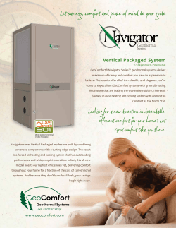


© Copyright 2026