Single-stage reconstruction algorithm for quantitative
photoacoustic tomography
arXiv:1501.04603v1 [math.AP] 19 Jan 2015
Markus Haltmeier♣ , Lukas Neumann♦ and Simon Rabanser♣♦
♣ Department
of Mathematics, University of Innsbruck
Technikestraße 13, A-6020 Innsbruck, Austria
♦ Institute
of Basic Sciences in Engineering Science, University of Innsbruck
Technikestraße 21a, A-6020 Innsbruck, Austria
E-mail: {markus.haltmeier,lukas.neumann,simon.rabanser}@uibk.ac.at
Abstract
The development of efficient and accurate image reconstruction algorithms is one of the
cornerstones of computed tomography. Existing algorithms for quantitative photoacoustic tomography currently operate in a two-stage procedure: First an inverse source problem for
the acoustic wave propagation is solved, whereas in a second step the optical parameters are
estimated from the result of the first step. Such an approach has several drawbacks. In
this paper we therefore propose the use of single-stage reconstruction algorithms for quantitative photoacoustic tomography, where the optical parameters are directly reconstructed
from the observed acoustical data. In that context we formulate the image reconstruction
problem of quantitative photoacoustic tomography as a single nonlinear inverse problem by
coupling the radiative transfer equation with the acoustic wave equation. The inverse problem is approached by Tikhonov regularization with a convex penalty in combination with the
proximal gradient iteration for minimizing the Tikhonov functional. We present numerical
results, where the proposed single-stage algorithm shows an improved reconstruction quality
at a similar computational cost.
Keywords. Quantitative photoacoustic tomography, stationary radiative transfer equation,
wave equation, single-stage algorithm, inverse problem, parameter identification
AMS classification numbers. 44A12, 45Q05, 92C55.
1
Introduction
Photoacoustic tomography (PAT) is a recently developed medical imaging paradigm that combines
the high spatial resolution of ultrasound imaging with the high contrast of optical imaging [7, 35,
52, 53, 54]. Suppose a semitransparent sample is illuminated with a short pulse of electromagnetic
energy near the visible range. Then parts of the optical energy will be absorbed inside the sample
which causes a rapid, non-uniform increase of temperature. The increase of temperature yields
a spatially varying thermoelastic expansion which in turn induces an acoustic pressure wave (see
Figure 1.1). The induced acoustic pressure wave is measured outside of the object of interest, and
mathematical algorithms are used to recover an image of the interior.
Original (and also a lot of recent) work in PAT has been concentrated on the problem of
reconstructing the initial pressure distribution, which has been considered as final image (see, for
1
Optical illumination
Thermal expansion
Acoustic pressure wave
Figure 1.1: Basic principle of PAT. A semitransparent sample is illuminated with a short
optical pulse. Due to optical absorption and subsequent thermal expansion within the sample an
acoustic pressure wave is induced. The acoustic pressure wave is measured outside of the sample
and used to reconstruct an image of the interior.
example, [1, 9, 24, 25, 26, 27, 30, 31, 37, 34, 38, 45, 50, 54]). However, the recovered pressure
distribution only provides indirect information about the investigated object. This is due to the
fact, that the initial pressure distribution is the product of the optical absorption coefficient and
the spatially varying optical intensity which again indirectly depends on the tissue parameters. As
a consequence, the initial pressure distribution only provides qualitative information about the
tissue-relevant parameters. Quantitative photoacoustic tomography (qPAT) addresses exactly
this issue and aims at quantitatively estimating the tissue parameters by supplementing the
wave inversion with an inverse problem for the light propagation in tissue (see, for example,
[2, 5, 6, 10, 15, 16, 14, 19, 36, 39, 41, 44, 46, 47, 51, 56]).
To the best of our knowledge, all existing reconstruction algorithms for qPAT are currently
performed via the following two-stage procedure: First, the measured pressure values are used to
recover the initial pressure distribution caused by the thermal heating. In a second step, based
on an appropriate light propagation model, the spatially varying tissue parameters are estimated
from the initial pressure distribution recovered in the first step. However, any algorithm for solving
an inverse problem requires prior knowledge abut the parameters to be recovered as well as partial
knowledge about the noise. If one approaches qPAT via a two-stage approach, appropriate prior
information for the acoustic inverse problem is difficult to model, because the initial pressure
depends on parameters not yet recovered. This is particularly relevant for the case that the
acoustic data can only be measured on parts of the boundary (limited-angle scenario), in which
case the acoustic inverse problems is known to be severely ill-posed. Further, using a two-stage
approach, only limited information about the noise for the optical problem is available.
In view of such shortcomings of the two-stage approach, in this paper we propose to recover
the optical parameters directly from the measured acoustical data via a single-stage procedure.
We work with the stationary radiative transfer equation (RTE) as model for light propagation.
Our simulations show improved reconstruction quality of the proposed single-stage algorithm at
a computational cost similar to the one of existing single-stage algorithms. Obviously our singlestage strategy can alternatively be combined with the diffusion approximation, which has also
frequently been used in qPAT. Here we use the stationary RTE since it is the more realistic model
for light propagation in tissue.
2
1.1
Mathematical modeling of qPAT
Throughout this paper, let Ω ⊂ Rd denote a convex bounded domain with Lipschitz-boundary
∂Ω, where d ∈ {2, 3} denotes the spatial dimension. We model the optical radiation by a function
Φ : Ω × Sd−1 → R, where Φ (x, θ) is the density of photons at location x ∈ Ω propagating in
direction θ ∈ Sd−1 . The photon density is supposed to satisfy the stationary radiative transfer
equation (RTE)
θ · ∇x Φ (x, θ) + (σ (x) + µ (x)) Φ (x, θ)
Z
k θ, θ ′ Φ(x, θ ′ )dθ ′ + q(x, θ)
= σ (x)
Sd−1
for (x, θ) ∈ Ω × Sd−1 . (1.1)
Here σ (x) is the scattering coefficient, µ (x) is the absorption coefficient, and q (x, θ) is the photon
source density. The scattering kernel k (θ, θ ′ ) describes the redistribution of velocity directions of
scattered photons due to interaction with the background. The stationary RTE (1.1) is commonly
considered as a very accurate model for light transport in tissue (see, for example, [3, 18, 21, 33]).
In order to obtain a well-posed problem one has to impose appropriate boundary conditions.
For that purpose it is convenient to split the boundary Γ := ∂Ω × Sd−1 into inflow and outflow
boundaries,
n
o
Γ− := (x, θ) ∈ ∂Ω × Sd−1 : ν(x) · θ < 0 ,
n
o
Γ+ := (x, θ) ∈ ∂Ω × Sd−1 : ν(x) · θ > 0 ,
with ν(x) denoting the outward pointing unit normal at x ∈ ∂Ω. We then augment (1.1) by the
inflow boundary conditions
Φ|Γ− = f
for some f : Γ− → R .
(1.2)
Under physically reasonable assumptions it can be shown that the stationary RTE (1.1) together
with the inflow boundary conditions (1.2) is a well-posed problem. In Section 2.1 we apply a
recent result of [20] that guarantees the well-posedness of (1.1), (1.2) even in the presence of voids
(parts of the domain under consideration, where µ and σ vanish).
The absorption of photons causes a non-uniform heating of the tissue proportional to the total
amount of absorbed photons,
Z
Φ(x, θ)dθ for x ∈ Ω .
h (x) := µ(x)
Sd−1
The heating in turn induces an acoustic pressure wave p : Rd × (0, ∞) → R. The initial pressure
distribution is given by p( · , 0) = Γh, where Γ is the Gr¨
uneissen parameter describing the efficiency
of conversion of heat into acoustic pressure. For the sake of simplicity we consider the Gr¨
uneissen
parameter to be constant, known and rescaled to one. We further assume the speed of sound
to be constant and also rescaled to one. The photoacoustic pressure then satisfies the following
initial value problem for the standard wave equation,
 2
for (x, t) ∈ Rd × (0, ∞)

 ∂t p(x, t) − ∆p(x, t) = 0 ,
(1.3)
p (x, 0) = h(x) , for x ∈ Rd


d
∂t p (x, 0) = 0 ,
for x ∈ R .
The goal of qPAT is to reconstruct the parameters µ and σ from measurements of the acoustic
pressure p outside Ω.
3
1.2
The inverse problem of qPAT
In the following we assume that acoustic measurements are available for multiple optical source
distributions (illuminations). For that purpose, let (qi , fi ) for i = 1, . . . N be given pairs of source
patterns and boundary data. We use Ti to denote the operator that takes the pair (µ, σ) to the
solution of the stationary RTE (1.1), (1.2) with qi and fi in place of q and f , and denote by
Z
Ti (µ, σ)(x, θ)dθ
for x ∈ Ω
Hi (µ, σ) (x) := µ(x)
Sd−1
the operator describing the corresponding thermal heating. Further, we write WΩ,Λ for the
operator that maps the initial data h to the solution WΩ,Λ h := p|∂Ω×(0,∞) of the wave equation
(1.3) restricted to the boundary ∂Ω. Appropriate functional analytic frameworks for Ti , Hi and
WΩ,Λ will be given in Section 2, where we also study properties of these mapping.
The reconstruction problem of qPAT with multiple illuminations can be written in the form
of a nonlinear inverse problem,
vi = (WΩ,Λ ◦ Hi ) (µ⋆ , σ ⋆ ) + zi
for i = 1, . . . , N .
(1.4)
Here vi are the measured noisy data, the operators WΩ,Λ ◦ Hi model the forward problem of
qPAT, zi are the noise in the data, and µ⋆ , σ ⋆ are the true parameters. The aim is to estimate
the parameter pair (µ⋆ , σ ⋆ ) from given data vi , and hence solving the inverse problem (1.4).
1.3
Outline of the paper
In this paper we address the inverse problem (1.4) by Tikhonov regularization,
N
1X
k(WΩ,Λ ◦ Hi ) (µ, σ) − vi k2 + λR(µ, σ) → min ,
2
(µ,σ)
i=1
where R is a convex penalty and λ > 0 is the regularization parameter. We show that Tikhonov
regularization applied to single-stage qPAT is well-posed and convergent; see Theorem 3.2. For
that purpose we derive regularity results for the heating operators Hi in Section 2. To establish
such properties we use results for the stationary RTE derived recently in [20].
For numerically minimizing the Tikhonov functional we apply the proximal gradient algorithm
(also named forward backward splitting); see Section 3.4. The proximal gradient algorithm,
is an iterative scheme for minimizing functionals that can be written as the sum of a smooth
and a convex part [13, 12]. For the classical two-stage approach in qPAT in combination with
the diffusion approximation, the proximal gradient algorithm has recently been applied in [58].
Numerical results using the proximal gradient algorithm applied to our single-stage approach
are presented in Section 4, where we also include a comparison with the two-stage approach.
Of course, our single-stage approach can be combined with classical gradient or Newton-type
schemes. The proximal gradient algorithm is our method of choice, since its is very flexible and
fast, and can be applied for a large class of smooth or non-smooth penalties.
2
Analysis of the direct problem of qPAT
Before actually studying the inverse problem of qPAT we first make sure that the forward problem
is well-posed in suitable spaces and that the data depend continuously on the parameters we
4
intend to reconstruct. For that purpose we review a recent existence and uniqueness result for
the stationary RTE allowing for voids in the domain of interest [20]. The use of a-priori estimates
will lead to differentiability results for the operators Ti and Hi .
2.1
The stationary RTE
The stationary RTE has been studied in various contexts. The most prominent, apart from the
transport of radiation in a scattering media, is reactor physics, where the equation is used in
the group velocity approximation of the neutron transport problem. An extensive collection of
results regarding applications as well as existence and uniqueness of solutions can be found in
[18]. The analysis of the RTE becomes considerably more involved if internal voids, i.e. regions
where scattering and absorption coefficient become zero, are allowed.
Suppose 1 ≤ p ≤ ∞, and denote by Lp (Γ− , |ν · θ|) the space of all measurable functions f
defined on Γ− for which
( qR
p
p
if p < ∞
Γ− |ν(x) · θ| |f (x, θ)| d(x, θ)
kf kLp (Γ− ,|ν·θ|) :=
ess sup(x,θ)∈Γ− {|ν(x) · θ| |f (x, θ)|} if p = ∞
is finite. We write W p (Ω × Sd−1 ) for the space of all measurable functions defined on Ω × Sd−1
such that
p
kΦkpW p (Ω×Sd−1 ) := kΦkpLp (Ω×Sd−1 ) + kθ · ∇x ΦkpLp (Ω×Sd−1 ) + Φ|Γ− Lp (Γ− ,|ν·θ|)
is well defined and finite (with the usual modification for p = ∞). The subspace of all Φ ∈
W p (Ω × Sd−1 ) with Φ|Γ− = 0 will be denoted by W0p (Ω × Sd−1 ). Further, for a given scattering
kernel k ∈ L∞ (Sd−1 × Sd−1 ) we write K : Lp (Ω × Sd−1 ) → Lp (Ω × Sd−1 ) for the corresponding
scattering operator,
Z
k(θ, θ ′ )Φ(x, θ ′ )dθ ′
for (x, θ) ∈ Ω × Sd−1 .
(KΦ) (x, θ) =
Sd−1
Throughout
R this article, the scattering kernel k is supposed to be symmetric and nonnegative, and
to satisfy Sd−1 k (θ, θ ′ ) dθ ′ = 1 for all θ ∈ Sd−1 . This reflects the fact that k ( · , θ ′ ) is a probability
distribution describing the redistributions of velocity directions due to interaction of the photons
with the background. Under these assumption, the scattering operator K is easily seen to be
linear and bounded.
Using the notation just introduced, the stationary RTE (1.1), (1.2) can be written in the
compact form
(
(θ · ∇x + (µ + σ − σK)) Φ = q in Ω × Sd−1
(2.1)
Φ|Γ− = f on Γ− .
By definition, a solution of the stationary RTE (1.1), (1.2) in W p is any function Φ ∈ W p (Ω ×
Sd−1 ) satisfying (2.1). The following theorem which has been derived very recently in [22] states
that under physically reasonable assumptions there exists exactly one such solution, that further
continuously depends on the source and the boundary data.
Theorem 2.1 (Existence and uniqueness of solutions in W p ). Let µ, σ denote positive constants,
let µ, σ be measurable functions satisfying 0 ≤ µ ≤ µ and 0 ≤ σ ≤ σ, and let 1 ≤ p ≤ ∞. Then,
for any source pattern q ∈ Lp (Ω × Sd−1 ) and all boundary data f ∈ Lp (Γ− , |ν · θ|), the stationary
5
RTE (1.1), (1.2) admits a unique solution Φ ∈ W p (Ω × Sd−1 ). Moreover, there exists a constant
Cp (µ, σ) only depending on p, µ and σ, such that the following a-priori estimate holds
kΦkpW p (Ω×Sd−1 ) ≤ Cp (µ, σ) kqkLp (Ω×Sd−1 ) + kf kLp (Γ− ,|ν·θ|) .
(2.2)
Proof. See [22].
2.2
The parameter-to-solution operator T for the stationary RTE
Throughout this subsection, let 1 ≤ p ≤ ∞, and let q ∈ L∞ (Ω × Sd−1 ) and f ∈ L∞ (Γ− , |ν · θ|)
be given source pattern and boundary data, respectively. Further, for fixed positive numbers
µ, σ > 0 we denote
Dp := {(µ, σ) ∈ Lp (Ω) × Lp (Ω) : 0 ≤ σ ≤ σ and 0 ≤ µ ≤ µ} .
(2.3)
Then Dp is a closed, bounded and convex subset of Lp (Ω) × Lp (Ω), that has empty interior in
the case that p < ∞.
Definition 2.2 (Parameter-to-solution operator for the stationary RTE). The parameter-tosolution operator for the stationary RTE is defined by
T : Dp → W p (Ω × Sd−1 ) : (µ, σ) 7→ Φ ,
(2.4)
where Φ denotes the unique solution of (1.1), (1.2).
According to Theorem 2.1 the operator T is well defined. Note further, that T depends on
p, q, f , µ and σ. Since these parameters will be fixed in the following and in order to keep the
notation simple we will not indicate the dependence of T these parameter explicitly.
Now we are in the position to state continuity properties of T derived in [21]. We include
a short proof of these results as its understanding is very useful for the derivation of similar
properties of the operator describing the heating that we investigate in the following subsection.
Theorem 2.3 (Lipschitz continuity and weak continuity of T).
(a) The operator T is Lipschitz-continuous.
(b) If 1 < p < ∞, then T is sequentially weakly continuous.
µ, σ
ˆ ) ∈ Dp be two given pairs of absorption and scattering coefficients and
Proof. (a) Let (µ, σ), (ˆ
ˆ := T(ˆ
denote by Φ := T(µ, σ) and Φ
µ, σ
ˆ ) the corresponding solutions of the stationary RTE.
∞
d−1
∞
ˆ −Φ
Since q ∈ L (Ω × S ) and f ∈ L (Γ− , |ν · θ|), Theorem 2.1 implies that the difference Φ
d−1
∞
is an element of W0 (Ω × S ). Further, this difference is easily seen to satisfy
ˆ − Φ) = (µ − µ
ˆ + (σ − σ
ˆ − (σ − σ
ˆ.
(θ · ∇x + µ + σ − σK) (Φ
ˆ) Φ
ˆ )Φ
ˆ ) KΦ
Because K is a bounded linear operator on Lp (Ω×Sd−1 ), the right hand side in the above equation
is actually contained in Lp (Ω × Sd−1 ). Therefore, a further application of Theorem 2.1 yields
ˆ
ˆ
ˆkLp (Ω×Sd−1 ) + kI − Kkp kσ − σ
ˆ kLp (Ω×Sd−1 ) ,
kΦ−Φk
W p (Ω×Sd−1 ) ≤ Cp (µ, σ)kΦkL∞ (Ω×Sd−1 ) kµ − µ
ˆ ∞
where I denotes the identity and k · k p the operator norm on Lp (Ω × Sd−1 ). Since kΦk
L (Ω×Sd−1 )
ˆ
is bounded independently of Φ, this implies the Lipschitz continuity of T.
6
(b) Let (µn , σn )n∈N be a sequence in Dp that converges weakly to the pair (µ, σ) ∈ Dp , and
denote by Φn = T(µn , σn ) and Φ = T(µ, σ) the corresponding solutions of the stationary RTE.
As in (a), one argues that the difference Φn − Φ is contained in W0∞ (Ω × Sd−1 ) and satisfies
(θ · ∇x + µ + σ − σK) (Φn − Φ) = (µ − µn ) Φn + (σ − σn )Φn − (σ − σn ) KΦn .
Now, from Theorem 2.1 it follows that θ · ∇x + µ + σ − σK is invertible as an operator from
W0p (Ω × Sd−1 ) to Lp (Ω × Sd−1 ). Consequently, the inverse mapping (θ · ∇x + µ + σ − σK)−1
is linear and bounded and in particular weakly continuous. It therefore remains to show that
(µ − µn ) Φn + (σ − σn )Φn − (σ − σn ) KΦn weakly converges to zero in Lp (Ω × Sd−1 ). To see this,
denote by p∗ = p/(p − 1) the dual index and let ϕ ∈ Lp∗ (Ω × Sd−1 ) be any element in the dual of
Lp Ω × Sd−1 . By Fubini’s theorem we have
Z
Z
Z
Φn (x, θ)ϕ(x, θ) dθ dx .
(µ(x) − µn (x))
(µ(x) − µn (x)) Φn (x, θ)ϕ(x, θ) d(x, θ) =
Ω×Sd−1
Sd−1
Ω
p∗
The averaging lemma (see,
R for example, [40]) implies that the averaging operator A : W (Ω ×
d−1
p
∗
S ) → L (Ω) : Φ 7→ Sd−1 Φ( · , θ)dθ is compact for 1 < Rp∗ < ∞. Since (Φn )n∈N is bounded
d−1
∞
d−1
p∗
in
R W (Ω × S ) ⊂ W (Ω × S ), this implies that Sd−1 Φn ( · , θ)ϕ( · , θ)dθ converges to
Sd−1 Φ( · , θ)ϕ( · , θ)dθ with respect to k · k Lp∗ (Ω) . As µn ⇀ µ we can conclude that (µ − µn )Φn
converges to zero weakly. In the same manner one shows (σ − σn ) Φn ⇀ 0. Finally, the equality
Z
Z
Z
Φn (x, θ)(Kϕ)(x, θ)dθdx
(µ − µn ) (x)
(µ − µn ) (x)(KΦn )(x, θ)ϕ(x, θ)d(x, θ) =
Ω×Sd−1
Sd−1
Ω
and the use of similar arguments show that (σ − σn ) KΦn ⇀ 0.
For the solution of the inverse problem of qPAT we will make use the derivative of T that we
compute next. For that purpose we call h ∈ Lp (Ω × Sd−1 ) × Lp (Ω × Sd−1 ) a feasible direction at
(µ, σ) ∈ Dp if there exists some ǫ > 0 such that (µ, σ) + ǫh ∈ Dp . Due to the convexity of Dp we
have u + sh ∈ Dp for all 0 < s ≤ ǫ. The set of all feasible directions will be denoted by Dp (µ, σ).
One immediately sees that
Dp (µ, σ) = Lp (Ω × Sd−1 ) × Lp (Ω × Sd−1 )
if 0 < µ < µ and 0 < σ < σ .
For (µ, σ) ∈ Dp and any feasible direction h ∈ Dp (µ, σ) we denote the one-sided directional
derivative of T at (µ, σ) in direction h by
T′ (µ, σ)(h) := lim
s↓0
T((µ, σ) + sh) − T(µ, σ)
,
s
(2.5)
provided that the limit on the right hand side of (2.5) exists. If both limits T′ (µ, σ)(h) and
T′ (µ, σ)(−h) exist and h 7→ T′ (µ, σ)(h) is bounded and linear, we say that T is Gˆ
ataux differen′
tiable at (µ, σ) and call T (µ, σ) the Gˆ
ataux derivative of T at (µ, σ).
Theorem 2.4 (Differentiability of T). For any (µ, σ) ∈ Dp , the one-sided directional derivative
of T at (µ, σ) in direction (hµ , hσ ) ∈ Dp (µ, σ) exists. Further, we have T′ (µ, σ)(hµ , hσ ) = Ψ,
where Ψ is the unique solution of
(
(θ · ∇x + (µ + σ − σK)) Ψ = − (hµ + hσ − hσ K) T(µ, σ) in Ω × Sd−1
(2.6)
Ψ|Γ− = 0
on Γ− .
ateaux differentiable at (µ, σ).
If 0 < µ < µ and 0 < σ < σ, then T is Gˆ
7
Proof. Suppose (µ, σ) ∈ Dp and let h = (hµ , hσ ) ∈ Dp (µ, σ) be any feasible direction. For
sufficiently small s > 0 write Φs := T((µ, σ) + sh) and Φ := T(µ, σ). As in the proof of Theorem
2.3 one shows that Ψs := (Φs − Φ)/s is contained in W0p (Ω × Sd−1 ) and solves the equation
(θ·∇x +µ+σ−σK)Ψs = −(hµ +hσ −hσ K)Φs . Consequently the difference Ψs −Ψ ∈ W0p (Ω×Sd−1 )
solves
(θ · ∇x + µ + σ − σK) (Ψs − Ψ) = −(hµ + hσ − hσ K)(Φs − Φ) .
Application of the a-priori estimate of Theorem 2.1 shows the inequality kΨs − ΨkW p (Ω×Sd−1 ) ≤
Cp (µ, σ)kΦs − ΦkL∞ (Ω×Sd−1 ) (khµ kLp (Ω×Sd−1 ) + khσ kLp (Ω×Sd−1 ) ) Together with the continuity of T
this implies that the one-sided directional derivative T′ (µ, σ)(h) exists and is given by lims→0 Ψs =
Ψ. Finally, if 0 < µ < µ and 0 < σ < σ, then h 7→ T′ (µ, σ)(h) is bounded and linear and therefore
T is Gˆ
ateaux differentiable at (µ, σ).
Note that for any parameter pair (µ, σ) ∈ Dp , the solution of (2.6) depends linearly and
continuously on (hµ , hσ ) ∈ Lp (Ω) × Lp (Ω). As a consequence, the one-sided directional derivative
can be extended to a bounded linear operator
T′ (µ, σ) : Lp (Ω) × Lp (Ω) → W p (Ω × Sd−1 ) : (hµ , hσ ) 7→ Ψ ,
(2.7)
where Ψ is the unique solution of (2.6). We will refer to this extension as the derivative of T at
(µ, σ).
2.3
The operator H describing the heating
Throughout this subsection, let q ∈ L∞ (Ω×Sd−1 ) and f ∈ L∞ (Γ− , |ν · θ|) be given source pattern
and boundary data, respectively. As already mentioned in the introduction, photoacoustic signal
generation due to the absorption of light is described by the operator
Z
p
T(µ, σ)( · , θ)dθ .
H : Dp → L (Ω) : (µ, σ) 7→ µ
Sd−1
To shorten the notation, in the following
we will make use of the averaging operator A : W p (Ω ×
R
d−1
p
S ) → L (Ω) defined by AΦ = Sd−1 Φ( · , θ)dθ. By H¨olders inequality the averaging operator is
well defined, linear and bounded. Using the averaging operator we can write H(µ, σ) = µAT(µ, σ).
Theorem 2.5 (Lipschitz continuity and weak continuity of H).
(a) The operator H is Lipschitz continuous.
(b) For 1 < p < ∞, H is sequentially weakly continuous.
µ, σ
ˆ ) ∈ Dp are two pairs of admissible absorption and scattering
Proof. (a) Suppose that (µ, σ), (ˆ
coefficients. The decomposition H(µ, σ) = µAT(µ, σ) and the triangle inequality imply
kµAT(µ, σ) − µ
ˆAT(ˆ
µ, σ
ˆ )kLp (Ω)
= kµAT(µ, σ) − µ
ˆAT(µ, σ) + µ
ˆAT(µ, σ) − µ
ˆAT(ˆ
µ, σ
ˆ )kLp (Ω)
≤ kAT(µ, σ)kL∞ (Ω) kµ − µ
ˆkLp (Ω) + kˆ
µkL∞ (Ω) kAT(µ, σ) − AT(ˆ
µ, σ
ˆ )kLp (Ω) .
According to Theorem 2.3, the operator T is Lipschitz continuous. Because A is linear and
bounded, also the composition AT is Lipschitz. Noting that kAT(µ, σ)kL∞ (Ω) and kˆ
µkL∞ (Ω) are
bounded by constants independent of µ, σ and µ
ˆ, σ
ˆ , this implies the Lipschitz continuity of H.
8
(b) Let (µn , σn )n∈N be a sequence in Dp that converges weakly to (µ, σ) ∈ Dp . Since T is
weakly continuous and A is linear and bounded, (AT(µn , σn ))n∈N converges weakly to AT(µ, σ).
Further, for any function ϕ ∈ Lp⋆ (Ω), the dual space of Lp (Ω), we have
Z
(µ(x)(AT)(µ, σ)(x) − µn (x)(AT)(µn , σn )(x)) ϕ(x) dx
Ω
Z
≤ kAT(µ, σ)kL∞ (Ω) (µ(x) − µn (x)) ϕ(x) dx
Z Ω
+ kµn kL∞ (Ω) ((AT)(µ, σ)(x) − (AT)(µn , σn )(x)) ϕ(x)dx .
Ω
The weak convergence of µn and (AT(µn , σn ))n∈N therefore implies the weak convergence of
µn AT(µn , σn ) to µAT(µ, σ) and shows the weak continuity of H.
Note that for the case 1 < p < ∞, the averaging operator A is even compact (see [40]) which
implies the compactness of the composition AT. As a consequence, for any given µ, the partial
mapping σ 7→ µ(AT)(µ, σ) is compact. It seems unlikely, however, that the full operator H is
compact, too.
Theorem 2.6 (Differentiability of H). For any (µ, σ) ∈ Dp , the one-sided directional derivative
of H at (µ, σ) in any feasible direction (hµ , hσ ) ∈ Dp (µ, σ) exists. Further, we have
Z
Z
′
T′ (µ, σ)(hµ , hσ )( · , θ)dθ ,
(2.8)
T(µ, σ)( · , θ)dθ + µ
H (µ, σ)(hµ , hσ ) = hµ
Sd−1
Sd−1
where T′ (µ, σ)(hµ , hσ ) denotes the one-sides directional derivative of T at (µ, σ) in direction
ateaux differentiable at
(hµ , hσ ) given by (2.6). Finally, if 0 < µ < µ and 0 < σ < σ, then H is Gˆ
(µ, σ).
Proof. Let (µ, σ) ∈ Dp and let (hµ , hσ ) ∈ Dp (µ, σ) be a feasible direction. For sufficiently small
s > 0, we have
H((µ, σ) + s(hµ , hσ )) − H(µ, σ)
s
(µ + shµ )(AT) ((µ, σ) + s(hµ , hσ )) − µ(AT) (µ, σ)
=
s
(AT) ((µ, σ) + s(hµ , hσ )) − (AT) (µ, σ)
= hµ (AT) ((µ, σ) + s(hµ , hσ )) + µ
.
s
According to Theorem 2.3, the operator T is continuous and therefore the first term converges to
hµ (AT)(µ, σ) as s → 0. Because T is one-sided differentiable, see Theorem 2.4, the second term
converges to µAT′ (µ, σ)(hµ , hσ ). Finally, if 0 < µ < µ and 0 < σ < σ, then H′ (µ, σ)(h) is linear
and bounded in the argument h which implies the Gˆ
ateaux differentiability of H at (µ, σ).
Recall that for any (µ, σ) ∈ Dp , the derivative T′ (µ, σ) is bounded and linear. Therefore, the
right hand side of (2.8) depends linearly and continuously on (hµ , hσ ) ∈ Lp (Ω) × Lp (Ω). As a
consequence, the one-sided directional derivative of H at (µ, σ) can be extended to a bounded
linear operator H′ (µ, σ) : Lp (Ω)×Lp (Ω) → Lp (Ω). We will refer to this extension as the derivative
of H at (µ, σ). The derivative of H can be written in the form H′ (µ, σ)(h) = hµ A(T(µ, σ)) +
µA(T′ (µ, σ)(h)).
9
2.4
The wave operator WΩ,Λ
¯ ⊂U
Let U ⊂ Rd be a bounded and convex domain with smooth boundary. We assume that Ω
and write L2Ω (Rd ) for the space of all square integrable functions defined on Rd that are supported
¯ Likewise we denote by C ∞ (Rd ) the space of all infinitely differentiable functions defined
in Ω.
Ω
¯ Further, let Λ ⊂ ∂U be a relatively open subset of ∂U , and denote
on Rd having support in Ω.
by diam(U ) the maximal diameter of U and by dist(Ω, Λ) the minimal distance of Ω from the
observation surface Λ.
Definition 2.7 (The wave operator WΩ,Λ ). Let wΩ,Λ : (0, ∞) → R be a smooth, nonnegative,
compactly supported function with wΩ,Λ (t) = 1 for all dist(Ω, Λ) ≤ t ≤ diam(U ) − dist(Ω, Λ). We
then define the wave operator by
WΩ,Λ : CΩ∞ (Rd ) ⊂ L2Ω (Rd ) → L2 (Λ × (0, ∞)) : h 7→ wΩ,Λ p|Λ×(0,∞) ,
(2.9)
where p denotes the unique solution of (1.3).
The operator WΩ,Λ maps the initial data of the wave equation (1.3) to its solution restricted
to Λ ⊂ ∂U and models the acoustic part of the forward problem of PAT. The cutoff function
wΩ,Λ accounts for the fact, that in the two dimensional case the solution of the wave equation has
unbounded support in time but measurements can only be made over a finite time interval.
In the following we use a result from [42] to show that WΩ,Λ is a bounded linear and densely
defined operator, and therefore can be extended to a bounded linear operator on L2Ω (Rd ) in a
unique manner.
Theorem 2.8 (Continuity of the wave operator WΩ,Λ ). There exists some constant cΩ,Λ such that
kWΩ,Λ hkL2 (Λ×(0,∞)) ≤ cΩ,Λ khkL2 (Rd ) for all h ∈ CΩ∞ (Rd ). Consequently, there exists a unique
Ω
bounded linear extension
WΩ,Λ : L2Ω (Rd ) → L2 (Λ × (0, ∞))
with WΩ,Λ |CΩ∞ (Rd ) = WΩ,Λ .
With some abuse of notation we again write WΩ,Λ for WΩ,Λ in the sequel.
Proof. It is sufficient to consider the case when the data are measured on the whole boundary
Λ = ∂U . The well known explicit formulas for the solution of (1.3) in two and three spatial
dimensions (see, for example, [23, 32]) imply that for every (y, t) ∈ ∂U × (0, ∞) we have
( w (t) R t
R
Ω,Λ
∂t 0 √t2r−r2 Sd−1 h (y + rω) dωdr for d = 2
2π
(WΩ,Λ h) (y, t) = wΩ,Λ (t)
(2.10)
R
∂t t Sd−1 h (y + tω) dω
for d = 3 .
4π
∞
d
∞
We define
R the spherical mean Radon transform M : CΩ (R ) → C (∂U × (0, ∞)) by Mh (y, t) :=
1/ωd−1 Sd−1 h(y + tω)dω for (y, t) ∈ ∂U × (0, ∞). With the spherical mean Radon transform, the
√
Rt
wave operator can be written as (WΩ,Λ h) (y, t) = wΩ,Λ (t) ∂t 0 rMh (y, r) / t2 − r 2 dr in the case
of two spatial dimensions and (WΩ,Λ h) (y, t) = wΩ,Λ (t) ∂t (tMh) (y, t) in the three dimensional
case.
Next we use a Sobolev estimate derived in [42], which states that for every λ ∈ R there
exists a constant cK,λ such that kMhkH λ+(d−1)/2 (∂U ×(0,∞)) ≤ cK,λ khkH λ (U ) for any h ∈ CΩ∞ (Rd ).
Application of this identity with λ = 0 and using the smoothing properties of the Abel transform
by degree 1/2 for the case of two spatial dimensions yields the continuity of WΩ,Λ with respect
to the L2 topologies. In particular, WΩ,Λ has a unique bounded linear extension to L2Ω (Rd ).
10
For solving the inverse problem of qPAT we will further require an explicit expression for the
adjoint of WΩ,Λ , that we compute next.
Proposition 2.9 (Adjoint of the wave operator). For v ∈ L2 (Λ × (0, ∞)) ∩ C 1 (Λ × (0, ∞)), and
¯ we have
every x ∈ Ω,

Z Z ∞
∂t (wΩ,Λ v) (y, t)
1

−
p
dr dS(y) if d = 2

2π Λ |x−y| r 2 − |x − y|2
∗
Z
(2.11)
WΩ,Λ v (x) =
∂t (wΩ,Λ v) (y, |x − y|)
1


−
dS(y)
if d = 3 .
4π Λ
|x − y|
Proof. This is a simple application of Fubini’s theorem and the explicit expression for WΩ,Λ h
given in (2.10).
3
Single-stage approach to qPAT
In this section we solve the inverse problem of qPAT by a single-stage approach. Our setting
allows acoustic measurement for multiple sources. Such a strategy has been called multi-source
qPAT or multiple illumination qPAT (see [6, 17, 57]). For that purpose, throughout this section
qi ∈ L∞ (Ω × Sd−1 ) and fi ∈ L∞ (Γ− , |ν · θ|) for i = 1, . . . N denote given source patterns and
boundary data, respectively. Recall that Ω ⊂ Rd denotes a bounded convex domain with Lipschitz
boundary and Γ− denotes the inflow boundary consisting of all pairs (x, θ) ∈ ∂Ω × Sd−1 with
ν(x) · θ < 0.
Ω
U
Λ
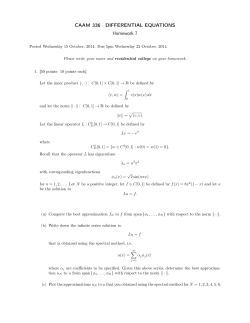
Figure 3.1: Setup for single-stage qPAT.
The stationary RTE governs the light propagation in the domain Ω. the absorption of photons
induces an initial pressure wave proportional to
¯ is supposed to
the heating Hi (µ, σ). Further, Ω
be contained in another domain U , and the pressure waves are measured with acoustic detectors
located on a open subset Λ ⊂ ∂U of the boundary of U .
To indicate the dependence of the solution of the stationary RTE on the pair (qi , fi ) we write
Ti : D2 → L2 (Ω × Sd−1 ) for the solution operator of the stationary RTE (1.1), (1.2) with sources
(qi , fi ). Here D2 is the set of all admissible pairs (µ, σ) defined in (2.3). Further, we use
Z
2
Ti (µ, σ)( · , θ)dθ
Hi : D2 → L (Ω) : (µ, σ) 7→ µ
Sd−1
to denote the corresponding operator describing the heating. For the coupling with the acoustic
problem, it will be convenient to consider Hi (µ, σ) ∈ L2 (Ω) as an element of L2Ω (Rd ), by extending
it to a function defined on Rd that is equal to zero on Rd \ Ω.
Further, recall the Definition 2.7 of the wave operator WΩ,Λ modeling the acoustic problem,
that maps the initial pressure h in the wave equation (1.3) to its solution restricted to Λ ⊂ ∂U .
11
Here U is a convex domain with smooth boundary that contains the support of f . To apply the
¯ ⊂ U . Then, according to the Section 2, the
results of Section 2, in the following we assume that Ω
operators Hi are Lipschitz continuous, weakly continuous and one-sided directional differentiable,
and WΩ,Λ is linear and bounded. A practical geometry of these domains is illustrated in Figure 3.1.
3.1
Formulation as operator equation
In order to apply standard techniques for the solution of inverse problems we write the reconstruction problem of (multiple-source) qPAT as a single operator equation. For that propose we
denote by
N
F : D2 → L2 (Λ × (0, ∞))
(µ, σ) 7→ (WΩ,Λ ◦ H1 (µ, σ), . . . , WΩ,Λ ◦ HN (µ, σ))
the operator describing the entire forward problem of qPAT. Further we denote by kvk2N :=
PN
2
2
N
i=1 kvi kL2 (Λ×(0,∞)) the squared standard norm on L (Λ × (0, ∞)) .
Theorem 3.1 (Properties of the forward operator of qPAT).
(a) The operator F sequentially weakly continuous.
(b) The operator F is Lipschitz continuous.
(c) For any (µ, σ) ∈ D2 , the one-sided directional derivative in any feasible direction h ∈
D2 (µ, σ) exists. Further,
F′ (µ, σ)(h) = WΩ,Λ ◦ H′1 (µ, σ)(h), . . . , WΩ,Λ ◦ H′N (µ, σ)(h)
(3.1)
where H′i (µ, σ)(h) is given by (2.8) with T replaced by Ti .
(d) If 0 < µ ≤ µ and 0 < σ < σ, then F is Gˆ
ateaux differentiable at (µ, σ).
Proof. All claims follow from the corresponding properties of the operators Hi (see Theorems 2.5
and 2.6) and the boundedness of WΩ,Λ discussed in Theorem 2.8.
The inverse problem of qPAT with multiple illuminations consists in solving the nonlinear
equation
v = F(µ⋆ , σ ⋆ ) + z ,
(3.2)
where (µ⋆ , σ ⋆ ) is the unknown, v = (v1 , . . . , vN ) are the given noisy data, F : D2 → L2 (Λ×(0, ∞))N
is the forward operator, and z is the noise in the data. Our single-stage approach for qPAT consists
in estimating the parameter pair (µ⋆ , σ ⋆ ) directly from (3.2). In contrast, existing two-stage
approaches for qPAT first construct estimates hi for the heating functions Hi (µ⋆ , σ ⋆ ) from data
vi by numerically inverting WΩ,Λ , and subsequently solve (h1 , . . . hN ) = (H1 (µ, σ), . . . , HN (µ, σ))
for (µ, σ).
There are at least two common methods for tackling an inverse problem of the form (3.2):
Tikhonov type regularization methods on the one and iterative regularization methods on the
other hand. In the following we apply Tikhonov regularization to the inverse problem of qPAT.
12
3.2
Tikhonov regularization for single-stage qPAT
We address the inverse problem (3.2) by Tikhonov regularization with general convex penalty.
For that purpose, let R : L2 (Ω) × L2 (Ω) → R ∪ {∞} be a convex, and lower semicontinuous
functional with domain D(R) := {(µ, σ) ∈ L2 (Ω) × L2 (Ω) : R(µ, σ) < ∞}. We assume that R is
chosen such that D2 ∩ D(R) is non-empty.
Tikhonov regularization with penalty R consists in computing a minimizer of the generalized
Tikhonov functional
Tv,λ : L2 (Ω) × L2 (Ω) → R ∪ {∞}
(
1
kF(µ, σ) − vk2N + λR(µ, σ)
(µ, σ) 7→ 2
∞
if (µ, σ) ∈ D2 ∩ D(R)
otherwise .
(3.3)
Here λ > 0 is the so called regularization parameter which has to be chosen accordingly, to balance
between stability with respect to noise and accuracy in the case of exact data. The data-fidelity
term 12 kF(µ, σ) − vk2N guarantees that any minimizer of (3.3) predicts the given data sufficiently
well. The regularization term λR(µ, σ) on the other hand avoids over-fitting of the data and
makes the reconstruction process well-defined and stable.
Note that Tikhonov regularization with penalty R is designed to stably approximate a solution
of the constrained optimization problem
R(µ, σ) →
such that F(µ, σ) = v ⋆ .
min
(µ,σ)∈D2 ∩D(R)
(3.4)
Here v ⋆ ∈ ran(F) is an element in the range of F and is referred to as exact data. Any solution of
(3.4) is called R-minimizing solution of the equation F(µ, σ) = v ⋆ . Under the given assumptions
there exists at least one R-minimizing solution, which however is not necessarily unique, see
[48, 49].
The properties of the operator F derived above and the use of general results from regularization theory yield the following result.
Theorem 3.2 (Well-posedness and convergence of Tikhonov regularization).
(a) For data v ∈ L2 (Λ × (0, ∞))N and every λ > 0, the Tikhonov functional Tv,λ has at least
one minimizer.
(b) Let λ > 0, v ∈ L2 (Λ × (0, ∞))N , and let (vn )n∈N be a sequence in L2 (Λ × (0, ∞))N
with kv − vn kN → 0. Then every sequence of minimizers (µn , σn ) ∈ arg min Tvn ,λ has a
weekly convergent subsequence. Further, the limit u of every weekly convergent subsequence
(µτ (n) , στ (n) )n∈N is a minimizer (µ, σ) of Tλ,v and satisfies (µτ (n) , στ (n) ) → R(µ, σ) for
n → ∞.
(c) Let v ⋆ ∈ ran(F), let (δn )n∈N ⊂ (0, ∞) be a sequence converging to zero, and let (vn )n∈N ⊂ V
be a sequence of data with kv ⋆ − vn kN ≤ δn . Suppose further that (λn )n∈N ⊂ (0, ∞) satisfies
λn → 0 and δn2 /λn → 0 as n → ∞. Then the following hold:
• Every sequence (µn , σn ) ∈ arg min Tvk ,λk has a weakly converging subsequence.
• The limit of every weakly convergent subsequence (µτ (n) , στ (n) )n∈N of (µn , σn )n∈N is
an R-minimizing solution (µ⋆ , σ ⋆ ) of F(µ, σ) = v ⋆ and satisfies R(µτ (n) , στ (n) ) →
R(µ⋆ , σ ⋆ ).
• If the R-minimizing solution of F(µ, σ) = v ⋆ is unique, then (µn , σn ) ⇀ (µ⋆ , σ ⋆ ).
13
Proof. Since F is sequentially weakly continuous (see Theorem 3.1) and D2 is closed and convex,
this follows from general results of Tikhonov regularization with convex penalties, see for example,
[48, Thm. 3.3, Thm. 3.4, Thm. 3.5].
3.3
Gradient of the data-fidelity term
For numerically minimizing the Tikhonov functional we require the gradient of the data-fidelity
term
N
1X
1
kWΩ,Λ µATi (µ, σ) − vi k2L2 (Λ×(0,∞)) .
(3.5)
F(µ, σ) := kF(µ, σ) − vk2N =
2
2
i=1
Recall that vi ∈ L2 (Ω) are the given data, Ti is the solution operator for the stationary RTE with
source patterns qi and boundary data fi , A is the averaging operator, and WΩ,Λ is the solution
operator for the wave equation.
Let (µ, σ) ∈ D2 be some admissible pair of parameters and let (hµ , hσ ) 7→ F ′ (µ, σ)(hµ , hσ )
denote the one-sided directional derivative of F at (µ, σ). We define the gradient ∇F(µ, σ) of F
at (µ, σ) to be any element in L2 (Ω × Sd−1 ) × L2 (Ω × Sd−1 ) satisfying
h∇F(µ, σ), (hµ , hσ )iL2 (Ω×Sd−1 )2 = F ′ (µ, σ)(hµ , hσ )
for (hµ , hσ ) ∈ D2 (µ, σ) .
(3.6)
From Theorem 3.1 and the chain rule, it follows that F ′ (µ, σ)(hµ , hσ ) exists for any feasible
direction (hµ , hσ ) ∈ D2 (µ, σ). Further, in the case that µ and σ are strictly positive, we have
D2 (µ, σ) = L2 (Ω × Sd−1 ) × L2 (Ω × Sd−1 ), which implies that ∇F(µ, σ) is uniquely defined by
(3.6).
In order to compute the gradient we require a more explicit expression for the one-sided
directional derivative, that we shall derive next.
Proposition 3.3 (One-sided directional derivative of the data-fidelity term). Let (µ, σ) ∈ D2 be
an admissible pair of parameters and let (hµ , hσ ) ∈ D2 (µ, σ) be a feasible direction. Then we have
F ′ (µ, σ)(hµ , hσ ) =
N
X
i=1
∗
AΦi WΩ,Λ
[WΩ,Λ µATi (µ, σ) − vi ] − A(Φi Φ∗i ), hµ
+
N
X
i=1
L2 (Ω)
hA (−Φi Φ∗i + (KΦi )Φ∗i ) , hσ iL2 (Ω) , (3.7)
where Φi := Ti (µ, σ), and Φ∗i is the unique solution of the adjoint equation
∗
(−θ · ∇x + (µ + σ − σK)) Φ∗i = A∗ µWΩ,Λ
[WΩ,Λ µAΦi − vi ]
in Ω × Sd−1
(3.8)
satisfying the zero outflow boundary condition Φ∗ |Γ+ = 0.
Proof. Obviously it is sufficient to consider the case N = 1, where we write v, T, Φ and Φ∗ in
place of vi , Ti , Φi and Φ∗i . By (3.5) we have
F ′ (µ, σ)(hµ , hσ )
= WΩ,Λ µAT(µ, σ) − v, WΩ,Λ hµ AT(µ, σ) + WΩ,Λ µAT′ (µ, σ)(hµ , hσ ) L2 (Λ×(0,∞))
= hWΩ,Λ µAΦ − v, WΩ,Λ hµ AΦiL2 (Λ×(0,∞))
14
+ WΩ,Λ µAΦ − v, WΩ,Λ µAT′ (µ, σ)(hµ , hσ ) L2 (Λ×(0,∞))
∗
= AΦWΩ,Λ
[WΩ,Λ µAΦ − v] , hµ L2 (Ω)
∗
+ A∗ µWΩ,Λ
[WΩ,Λ µAΦ − v] , T′ (µ, σ)(hµ , hσ ) L2 (Ω×Sd−1 ) .
(3.9)
∗
[WΩ,Λ µAΦ − v] and
Recall that Φ∗ is the solution of (3.8) with source term q = A∗ µWΩ,Λ
∗
zero outflow boundary conditions Φ |Γ+ = 0. Further, according to Theorem 2.4, the one-sided
directional derivative of T is given by T′ (µ, σ)(hµ , hσ ) = Ψ, where Ψ is the unique solution of
(θ · ∇x + (µ + σ − σK))Ψ = −(hµ + hσ − hσ K)Φ with inflow boundary conditions Ψ|Γ− = 0. The
zero outflow and zero inflow boundary conditions of Φ∗ and Ψ, respectively, and one integration by
parts, show h−θ ·∇x Φ∗ , ΨiL2 (Ω×Sd−1 ) = hΦ∗ , θ ·∇x ΨiL2 (Ω×Sd−1 ) . Further, notice that the averaging
operator A has adjoint A∗ : L2 (Ω) → L2 (Ω × Sd−1 ), (A∗ g)(x, v) = g(x), and that the scattering
operator K is self-adjoint.
Using these considerations, the second term in (3.9) can be written as
∗
A∗ µWΩ,Λ
[WΩ,Λ µAΦ − v] , T′ (µ, σ)(hµ , hσ ) L2 (Ω×Sd−1 )
= h(−θ · ∇x + (µ + σ − σK)) Φ∗ , ΨiL2 (Ω×Sd−1 )
= hΦ∗ , (θ · ∇x + (µ + σ − σK)) ΨiL2 (Ω×Sd−1 )
= hΦ∗ , − (hµ + hσ − hσ K) ΦiL2 (Ω×Sd−1 )
= − hΦΦ∗ , hµ + hσ iL2 (Ω×Sd−1 ) + h(KΦ)Φ∗ , hσ iL2 (Ω×Sd−1 )
= − hΦΦ∗ , A∗ (hµ + hσ )iL2 (Ω×Sd−1 ) + h(KΦ)Φ∗ , A∗ hσ iL2 (Ω×Sd−1 )
= h−A(ΦΦ∗ ), hµ iL2 (Ω) + h−A(ΦΦ∗ ) + A((KΦ)Φ∗ ), hσ iL2 (Ω) .
Together with (3.9) this yields the desired identity (3.7).
Let (µ, σ) ∈ D2 be an admissible pair of absorption and scattering coefficient. If µ, σ are
both strictly positive, then one concludes from Proposition 3.3 that the gradient of F at (µ, σ) is
uniquely defined and given by ∇F(µ, σ) = (∇µ F(µ, σ), ∇σ F(µ, σ)) with
∇µ F(µ, σ) =
∇σ F(µ, σ) =
N
X
i=1
N
X
∗
AΦi WΩ,Λ
[WΩ,Λ µAΦi − vi ] − A(Φi Φ∗i )
A (−Φi Φ∗i + (KΦi )Φ∗i ) .
(3.10)
(3.11)
i=1
Here Φi := Ti (µ, σ), and Φ∗i is the solution of the adjoint equation (3.8) with zero outflow
boundary condition. In the case that µ, σ are not both strictly positive, the gradient is not
uniquely defined by (3.6). However, Proposition 3.3 implies that the vector ∇F(µ, σ) defined
by (3.10), (3.11) still satisfies (3.3). We therefore take (3.10), (3.11) as gradient of F at any
(µ, σ) ∈ D2 .
3.4
Proximal gradient algorithm for single-stage qPAT
In order to minimize the Tikhonov functional we apply the proximal gradient (or forward backward
splitting) algorithm, which is an iterative algorithm for minimizing functionals that can be written
as a sum F + G, where F is smooth and G is convex [13, 12]. The proximal gradient algorithm
15
computes a sequence of iterates by alternating application of explicit gradient steps for the first
functional F and implicit proximal steps for the second functional G.
To apply the proximal gradient algorithm for minimizing the Tikhonov functional (3.3) we
take F(µ, σ) = 21 kF(µ, σ) − vk2N for the first and G(µ, σ) = λR(µ, σ) for the second functional.
The proximal gradient algorithm then generates a sequence (µn , σn ) of iterates defined by
(µn+1 , σn+1 ) := proxsn λR ((µn , σn ) − sn ∇F (µn , σn ))
for n ∈ N .
(3.12)
Here (µ0 , σ0 ) ∈ D2 ∩ D(R) is an initial guess, sn > 0 is the step size in the n-th iteration,
∇F(µ, σ) = (∇µ F(µ, σ), ∇σ F(µ, σ)) is the gradient of F given by (3.10), (3.11), and
proxsn λR (ˆ
σ, µ
ˆ) :=
1
k(µ, σ) − (ˆ
σ, µ
ˆ)k2 + sn λR(µ, σ)
2
(σ,µ)∈D2 ∩D(R)
arg min
(3.13)
is the proximity operator corresponding to the functional sn λR(µ, σ).
Remark 3.4 (Lipschitz continuity of ∇F). Note that the gradient ∇F of the data-fidelity term is
easily be shown to be Lipschitz continuous. This either can be deduced from the explicit expressions
(3.10), (3.11) or by using the expression ∇F(µ, σ) = F′ (µ, σ)∗ (F (µ, σ) − v). In any case, the
Lipschitz continuity of (µ, σ) 7→ ∇F(µ, σ) is shown similarly to proofs of the Lipschitz-continuity
of T and H, given in Section 2.2 and Section 2.3, respectively.
Convergence of the proximal gradient algorithm (3.12) is well known for the case that F is
convex with β-Lipschitz continuous gradient and that the chosen step sizes satisfy sn ∈ [ǫ, 2/β − ǫ]
for some constant ǫ > 0, see [13, 12]. These results are also valid for infinite dimensional Hilbert
spaces. Because our forward operator F is nonlinear, the data-fidelity term F is non-convex and
these results are not directly applicable to qPAT. Recently, the converge analysis of the proximal
gradient analysis has been extended to the case of non-convex functionals; see [4, 8, 11].
4
Numerical implementation
Our numerical simulations are carried out in d = 2 spatial dimensions. The stationary RTE is
solved on a square domain Ω = [0, 1]2 . For the scattering kernel we choose the two dimensional
version of the Henyey-Greenstein kernel,
k(θ, θ ′ ) :=
1 − g2
1
2π 1 + g 2 − 2g cos(θ · θ ′ )
for θ, θ ′ ∈ S1 ,
where g ∈ (0, 1) is the anisotropy factor. Before we present results of our numerical simulations
we first outline how we numerically solve the stationary RTE in two spatial dimensions that is
required for evaluating both, the forward operator F and the gradient ∇F of the data-fidelity
term.
4.1
Numerical solution of the RTE
For the numerical solution of the stationary RTE (1.1), (1.2) we employ a finite element method.
For that purpose one calculates the weak form of equation (1.1), (1.2) by integrating the equation
against a test function w : Ω × S1 → R. Integrating by parts in the transport term yields
Z Z
Z
Z Z
qw dθ dx . (4.1)
Φw (θ · ν) dσ =
(−θ · ∇x w + µw + σw − σKw) Φ dθ dx +
Ω
∂Ω×S1
S1
16
Ω
S1
Here we dropped all dependencies on the variables to shorten notation and dσ denotes the usual
surface measure on ∂Ω × S1 .
The numerical scheme replaces the exact solution by a linear combination in the finite element
space
Nh
X
(h) (h)
Φ(h) (x, θ) =
ci ψi (x, θ) ,
(4.2)
i=1
(h)
where any ψi (x, θ) is the product of a basis function in space and a basis function in velocity
and the sum ranges over all possible combinations. The spatial domain is triangulated uniformly
with mesh size h as illustrated in Figure 4.1. The velocity direction on the circle is divided into
16 equal subintervals. We use P1 Lagrangian elements, i.e. piecewise affine functions, in the two
dimensional spatial domain as well as for the angle.
x(N +1)2
x1
xN +1
Figure 4.1: Spatial finite element discretization. The square domain Ω = [0, 1]2 is
divided into 2N 2 triangles. To any of the (N +1)2
grid points x1 , . . . , x(N +1)2 a piecewise affine basis function is associated, that takes the value
one at one grid point and the value zero on all
other grid points, and is affine on every triangle.
To increase stability in low scattering areas we add some artificial diffusion in the transport
direction. This is called the streamline diffusion method, see for example [33] and the references
therein. In the streamline diffusion method the solution Φ is approximated in the usual way by
(4.2). However, the test functions take the form
w=
Nh
X
j=1
wj (ψj (x, θ) + δ(x) θ · ∇x ψj (x, θ)) ,
(4.3)
where the additional term introduces some artificial diffusion. In our experiments, the stabilization
parameter is taken as δ(x) = 3h/100 for σ(x) + µ(x) < 1 and zero otherwise. Note that the
streamline diffusion method provides a fully consistent stabilization of the original problem.
Making the ansatz (4.2) for the numerical solution and using test functions of the form (4.3),
equation (4.1) yields a system of linear equations M (h) c(h) = b(h) for the coefficient vector of
the numerical solution. The entries of M (h) and b(h) can be calculated by setting Φ = ψi and
w = ψj + δθ · ∇x ψj . For simplicity we only consider the case q = 0. Then, similar to (4.1) we
obtain
Z
Z Z
|θ · ν| ψi ψj dσ
(δθ · ∇x ψi − ψi ) θ · ∇x ψj dθdx +
Γ+
Ω S1
Z
Z Z
|θ · ν| ψi ψj dσ . (4.4)
(µ + σ − σK) (ψj + δθ · ∇x ψj ) ψi dθdx =
Ω
S1
Γ−
The entries of the matrix M (h) now can be calculated by evaluating the integrals on the left hand
side of (4.4). The right hand side of (4.4) together with the prescribed boundary values on Γ−
yields the entries of b(h) .
17
4.2
Numerical results
For the following numerical results, the stationary RTE is solved by the finite element method
outlined in Subsection 4.1. For that purpose the domain Ω = [0, 1]2 is discretized by a mesh
containing 7442 triangular elements (compare Figure 4.1). The angular domain is divided into 16
subintervals of equal length. The anisotropy factor is taken as g = 0.6 and the scattering coefficient
is taken as σ = 3. We use a single source distribution representing a planar illumination along
the lower edge [0, 1] × {0}.
The solution of the two-dimensional wave equation (1.3) is computed by numerically evaluating the solution formula (2.10), where the detection curve Λ = {3/2(cos ϕ, sin ϕ) : ϕ ∈ (−π, 0)} is
∗ h is evaluated by numerically implea half-circle on the boundary of B3/2 (0). The adjoint WΩ,Λ
menting (2.11). This can be done efficiently by a filtered backprojection algorithm as described
in [9, 25]. The geometry of Ω and Λ is similar to the one illustrated in Figure 3.1.
0.9
0.9
0.9
0.8
0.8
0.8
0.7
0.7
0.7
0.6
0.6
0.6
0.5
0.5
0.5
0.4
0.4
0.4
0.3
0.3
0.3
0.2
0.2
0.2
0.1
0.1
0.1
Figure 4.2: Reconstruction results for simulated data. True absorption coefficient (left),
reconstructed absorption coefficient using our single-stage approach (middle), and reconstructed
absorption coefficient using the usual two-stage approach (right).
For our initial experiments we assume the scattering coefficient σ to be known. In such a
situation, the proximal gradient algorithm outlined in the Subsection 3.4 reads
µn+1 := proxsn λR (µn − sn ∇µ F (µn , σ))
for n ∈ N
where sn > 0 is the step size, ∇µ F(µ, σ) is the gradient of F in the first component, given by (3.10),
and proxsn λR ( · ) is the proximity operator similar as in (3.13). In the presented numerical examples the regularization term is taken as a quadratic functional R(µ) = 21 k∂x µk2L2 (Ω) + 21 k∂y µk2L2 (Ω) .
In order to speed up the iterative scheme we compute the proximity operator only approximately
by projecting the unconstrained minimizer arg minµ 12 kµ − µ
ˆk2 + sn λR(µ) on D2 . Therefore the
main numerical cost in the proximal step the solution of a linear equation, which is relatively
cheap compared to the evaluation of the gradient ∇µ F.
In Figure 4.2 we present results of our numerical simulations. The left image shows the true
absorption coefficient and the central image shows the numerical reconstruction with the proposed
single-stage approach (using 40 iterations of the proximal gradient algorithm). For comparison
purpose, the right image in Figure 4.2 shows reconstruction results using the classical two-stage
approach. For that purpose we apply Tikhonov regularization and the proximal gradient algorithm
(again using 40 iterations) to the inverse problem h = Hi (µ) + zh . The approximate heating h is
computed numerically by applying the two dimensional universal backprojection formula [9, 38, 29]
the wave data v = WΩ,Λ ◦ Hi (µ) + z. All computations have been performed in Matlab on a
18
MacBook Pro with 2.3 GHz Intel Core i7 processor. The total computation times have been 26
minutes for the two-stage approach and 38 minutes for the single-stage approach.
One notices that in both reconstructions some boundaries in the upper half are blurred. Such
artifacts are expected and arise from the ill-posedness of the acoustical problem when using
limited-angle data; see [28, 43, 55]. However these artifacts are less severe for the single-stage
algorithm than for the classical two-stage algorithm. Further, in this example, the single-stage
algorithm also yields a better quantitative estimation of the values of the absorption coefficient.
0.14
0.9
0.9
0.12
0.8
0.8
0.7
0.7
0.6
0.6
0.5
0.5
0.4
0.4
0.3
0.3
0.2
0.2
0.1
0.1
0.1
0.08
0.06
0.04
0.02
0
−0.02
−0.04
−0.06
Figure 4.3: Reconstruction results for noisy data. Pressure data with 5% noise (left),
reconstructed absorption coefficient using our single-stage approach (middle) the classical twostage approach (right).
Finally, in order to investigate the stability of the derived algorithms with respect to noise,
we applied the single-stage and the two-stage algorithm after adding Gaussian white noise to the
data with standard deviation equal to 5% of the maximal absolute value of the pressure data.
The reconstruction results for noisy data are shown in Figure 4.3. As can be seen both algorithms
are quite stable with respect to data perturbations. However, again, the single-stage approach
yields better results and less artifacts than the two-stage algorithm.
5
Conclusion
In this paper we proposed a single-stage approach for quantitative PAT. For that purpose we derive
algorithms that directly recover the optical parameters from the measured acoustical data. This is
in contrast to the usual two-stage approach, where the absorbed energy distribution is estimated
in a first step, and the optical parameters are reconstructed from the estimated energy distribution
in a second step. Our single-stage algorithm is based on generalized Tikhonov regularization and
minimization of the Tikhonov functional by the proximal gradient algorithm. In order to show
that Tikhonov regularization is well-posed and convergent we analyzed the stationary radiative
transfer equation (1.1), (1.2) in a functional analytic framework. For that purpose we used recent
results of [20] that guarantees the well-posedness even in the case of voids.
We presented results of our initial numerical studies using a simple limited angle scenario,
where the scattering coefficient is assumed to be known. In this situation our single-stage algorithms has led to less artifacts than the two-stage procedure. More detailed numerical studies
will be presented in future work. In that context, we will also investigate the use of multiple
illuminations and multiple wavelength, which allows to also reconstruct the in general unknown
scattering coefficient Gr¨
uneissen parameter. We further plan to investigate the use of more general
regularization functionals such as the total variation in combination with the two-stage approach.
19
Acknowledgements
This work has been supported by the Tyrolean Science Fund (Tiroler Wissenschaftsfonds), project
number 153722.
References
[1] M. Agranovsky, P. Kuchment, and L. Kunyansky. On reconstruction formulas and algorithms for the
thermoacoustic tomography. In L. V. Wang, editor, Photoacoustic imaging and spectroscopy, chapter 8,
pages 89–101. CRC Press, 2009.
[2] H. Ammari, E. Bossy, V. Jugnon, and H. Kang. Reconstruction of the optical absorption coefficient
of a small absorber from the absorbed energy density. SIAM J. Appl. Math., 71(3):676–693, 2011.
[3] S. R. Arridge. Optical tomography in medical imaging. Inverse Probl., 15(2):R41–R93, 1999.
[4] H. Attouch, J. Bolte, and B. F. Svaiter. Convergence of descent methods for semi-algebraic and tame
problems: proximal algorithms, forward–backward splitting, and regularized Gauss–Seidel methods.
Math. Program., 137(1-2):91–129, 2013.
[5] G. Bal, A. Jollivet, and V. Jugnon. Inverse transport theory of photoacoustics. Inverse Probl.,
26:025011, 2010.
[6] G. Bal and K. Ren. Multi-source quantitative photoacoustic tomography in a diffusive regime. Inverse
Probl., 27(7):075003, 20, 2011.
[7] P. Beard. Biomedical photoacoustic imaging. Interface focus, 1(4):602–631, 2011.
[8] J. Bolte, S. Sabach, and M. Teboulle. Proximal alternating linearized minimization for nonconvex and
nonsmooth problems. Math. Program., 146(1-2, Ser. A):459–494, 2014.
[9] P. Burgholzer, J. Bauer-Marschallinger, H. Gr¨
un, M. Haltmeier, and G. Paltauf. Temporal backprojection algorithms for photoacoustic tomography with integrating line detectors. Inverse Probl.,
23(6):S65–S80, 2007.
[10] J. Chen and Y. Yang. Quantitative photo-acoustic tomography with partial data. Inverse Probl.,
28(11):115014 (15pp), 2012.
[11] E. Chouzenoux, J.-C. Pesquet, and A. Repetti. Variable metric forward-backward algorithm for
minimizing the sum of a differentiable function and a convex function. J. Optim. Theory Appl.,
162(1):107–132, 2014.
[12] P. L. Combettes and J.-C. Pesquet. Proximal splitting methods in signal processing. In Fixed-point
algorithms for inverse problems in science and engineering, pages 185–212. Springer, 2011.
[13] P. L. Combettes and V. R. Wajs. Signal recovery by proximal forward-backward splitting. Multiscale
Model. Sim., 4(4):1168–1200, 2005.
[14] B. Cox, J. G. Laufer, S. R. Arridge, and Paul C. Beard. Quantitative spectroscopic photoacoustic
imaging: a review. J. Biomed. Opt., 17(6):0612021, 2012.
[15] B. T. Cox, S. A. Arridge, and P. C. Beard. Gradient-based quantitative photoacoustic image reconstruction for molecular imaging. In Proc. SPIE 6437, page 64371T, 2007.
[16] B. T. Cox, S. R. Arridge, P. K¨
ostli, and P. C. Beard. Two-dimensional quantitative photoacoustic image reconstruction of absorption distributions in scattering media by use of a simple iterative method.
Appl. Opt., 45(8):1866–1875, 2006.
[17] B. T. Cox, T. Tarvainen, and S. R. Arridge. Multiple illumination quantitative photoacoustic tomography using transport and diffusion models. In G. Bal, D. Finch, P. Kuchment, J. Schotland,
P. Stefanov, and G. Uhlmann, editors, Tomography and Inverse Transport Theory, volume 559 of
Contemporary Mathematics, pages 1–12. AMS, 2011.
20
[18] R. Dautray and J. Lions. Mathematical analysis and numerical methods for science and technology.
Vol. 6. Springer-Verlag, Berlin, 1993.
[19] A. De Cezaro and T. F. De Cezaro. Regularization approaches for quantitative photoacoustic tomography using the radiative transfer equation. http://arXiv:1307.3201, 2013.
[20] H. Egger and M. Schlottbom. An Lp theory for stationary radiative transfer. Appl. Anal., 93(6):1283–
1296, 2014.
[21] H. Egger and M. Schlottbom. Numerical methods for parameter identification in stationary radiative
transfer. Comput. Optim. Appl., pages 1–17, 2014.
[22] H. Egger and M. Schlottbom. Stationary radiative transfer with vanishing absorption. Math. Models
Methods Appl. Sci., 24(5):973–990, 2014.
[23] L. C. Evans. Partial Differential Equations, volume 19 of Graduate Studies in Mathematics. Amer.
Math. Soc., Providence, RI, 1998.
[24] F. Filbir, S. Kunis, and R. Seyfried. Effective discretization of direct reconstruction schemes for
photoacoustic imaging in spherical geometries. SIAM J. Numer. Anal., 52(6):2722–2742, 2014.
[25] D. Finch, M. Haltmeier, and Rakesh. Inversion of spherical means and the wave equation in even
dimensions. SIAM J. Appl. Math., 68(2):392–412, 2007.
[26] D. Finch, S. K. Patch, and Rakesh. Determining a function from its mean values over a family of
spheres. SIAM J. Math. Anal., 35(5):1213–1240, 2004.
[27] D. Finch and Rakesh. The spherical mean value operator with centers on a sphere. Inverse Probl.,
23(6):37–49, 2007.
[28] J. Frikel and E. T. Quinto. Artifacts in incomplete data tomography - with applications to photoacoustic tomography and sonar. arXiv:1407.3453 [math.AP], 2014.
[29] M. Haltmeier. Inversion of circular means and the wave equation on convex planar domains. Comput.
Math. Appl., 65(7):1025–1036, 2013.
[30] M. Haltmeier. Universal inversion formulas for recovering a function from spherical means. SIAM J.
Math. Anal., 46(1):214–232, 2014.
[31] M. Haltmeier, T. Schuster, and O. Scherzer. Filtered backprojection for thermoacoustic computed
tomography in spherical geometry. Math. Method. Appl. Sci., 28(16):1919–1937, 2005.
[32] F. John. Partial Differential Equations, volume 1 of Applied Mathematical Sciences. Springer Verlag,
New York, fourth edition, 1982.
[33] G. Kanschat. Solution of radiative transfer problems with finite elements. In Numerical methods in
multidimensional radiative transfer, pages 49–98. Springer, Berlin, 2009.
[34] R. Kowar. On time reversal in photoacoustic tomography for tissue similar to water. SIAM J. Imaging
Sci., 7(1):509–527, 2014.
[35] R. A. Kruger, K. K. Kopecky, A. M. Aisen, Reinecke D. R., G. A. Kruger, and W. L. Kiser. Thermoacoustic ct with radio waves: A medical imaging paradigm. Radiology, 200(1):275–278, 1999.
[36] R. A Kruger, P. Lui, Y. R. Fang, and R. C. Appledorn. Photoacoustic ultrasound (PAUS) – reconstruction tomography. Med. Phys., 22(10):1605–1609, 1995.
[37] P. Kuchment and L. A. Kunyansky. Mathematics of thermoacoustic and photoacoustic tomography.
Eur. J. Appl. Math., 19:191–224, 2008.
[38] L. A. Kunyansky. Explicit inversion formulae for the spherical mean Radon transform. Inverse Probl.,
23(1):373–383, 2007.
21
[39] A. V. Mamonov and K. Ren. Quantitative photoacoustic imaging in radiative transport regime.
Comm. Math. Sci., 12(2):201–234, 2014.
[40] M. Mokthar-Kharroubi. Mathematical topics in neutron transport theory. World Scientific, 1997.
[41] W. Naetar and O. Scherzer. Quantitative photoacoustic tomography with piecewise constant material
parameters. SIAM J. Imaging Sci., 7(3):1755–1774, 2014.
[42] V. P. Palamodov. Remarks on the general Funk–Radon transform and thermoacoustic tomography.
Inverse Probl. Imaging, 4(4):693–702, 2010.
[43] G. Paltauf, R. Nuster, M. Haltmeier, and P. Burgholzer. Experimental evaluation of reconstruction
algorithms for limited view photoacoustic tomography with line detectors. Inverse Probl., 23(6):S81–
S94, 2007.
[44] K. Ren, H. Gao, and H. Zhao. A hybrid reconstruction method for quantitative PAT. SIAM J.
Imaging Sci., 6(1):32–55, 2013.
[45] A. Rosenthal, V. Ntziachristos, and D. Razansky. Acoustic inversion in optoacoustic tomography: A
review. Curr. Med. Imaging Rev., 9(4):318–336, 2013.
[46] A. Rosenthal, D. Razansky, and V. Ntziachristos. Fast semi-analytical model-based acoustic inversion
for quantitative optoacoustic tomography. IEEE Trans. Med. Imag., 29(6):1275–1285, 2010.
[47] T. Saratoon, T. Tarvainen, B. T. Cox, and S. R. Arridge. A gradient-based method for quantitative
photoacoustic tomography using the radiative transfer equation. Inverse Probl., 29(7):075006, 2013.
[48] O. Scherzer, M. Grasmair, H. Grossauer, M. Haltmeier, and F. Lenzen. Variational methods in
imaging, volume 167 of Applied Mathematical Sciences. Springer, New York, 2009.
[49] T. Schuster, B. Kaltenbacher, B. Hofmann, and K. S. Kazimierski. Regularization methods in Banach
spaces, volume 10 of Radon Series on Computational and Applied Mathematics. Walter de Gruyter,
Berlin, 2012.
[50] P. Stefanov and G. Uhlmann. Thermoacoustic tomography with variable sound speed. Inverse Probl.,
25(7):075011, 16, 2009.
[51] T. Tarvainen, B. T. Cox, J. P. Kaipio, and S. A. Arridge. Reconstructing absorption and scattering
distributions in quantitative photoacoustic tomography. Inverse Probl., 28(8):084009 (17pp), 2012.
[52] K. Wang and M. Anastasio. Photoacoustic and thermoacoustic tomography: Image formation principles. In Handbook of Mathematical Methods in Imaging, chapter 18, pages 781–815. Springer, 2011.
[53] L. V. Wang. Multiscale photoacoustic microscopy and computed tomography.
3(9):503–509, 2009.
Nat. Photonics,
[54] M. Xu and L. V. Wang. Photoacoustic imaging in biomedicine. Rev. Sci. Instrum., 77(4):041101
(22pp), 2006.
[55] Y. Xu, L. V. Wang, G. Ambartsoumian, and P. Kuchment. Reconstructions in limited-view thermoacoustic tomography. Med. Phys., 31(4):724–733, 2004.
[56] L. Yao, Y. Sun, and J. Huabei. Transport-based quantitative photoacoustic tomography: simulations
and experiments. Phys. Med. Biol., 55(7):1917–1934, 2010.
[57] R. J. Zemp. Quantitative photoacoustic tomography with multiple optical sources. Appl. Opt.,
49(18):3566–3572, 2010.
[58] X. Zhang, W. Zhou, X. Zhang, and H. Gao. Forward–backward splitting method for quantitative
photoacoustic tomography. Inverse Probl., 30(12):125012, 2014.
22