
Visualisation of Smoothed Particle
Visualisation of Smoothed Particle Hydrodynamics data using
SPLASH - v2.5.1
Daniel Price
January 29, 2015
Contents
1
Introduction
1.1 What it does . . . .
1.2 What it doesn’t do .
1.3 SPLASH , the paper
1.4 Version History . .
1.5 Licence . . . . . .
.
.
.
.
.
.
.
.
.
.
.
.
.
.
.
.
.
.
.
.
.
.
.
.
.
.
.
.
.
.
.
.
.
.
.
.
.
.
.
.
.
.
.
.
.
.
.
.
.
.
.
.
.
.
.
.
.
.
.
.
.
.
.
.
.
.
.
.
.
.
.
.
.
.
.
.
.
.
.
.
.
.
.
.
.
.
.
.
.
.
.
.
.
.
.
.
.
.
.
.
.
.
.
.
.
.
.
.
.
.
.
.
.
.
.
.
.
.
.
.
.
.
.
.
.
.
.
.
.
.
.
.
.
.
.
.
.
.
.
.
.
.
.
.
.
.
.
.
.
.
.
.
.
.
.
.
.
.
.
.
.
.
.
.
.
.
.
.
.
.
.
.
.
.
.
6
6
6
7
7
9
2
Getting started
2.1 Compiling the code . . . . . . . . . . . .
2.1.1 Fortran compilers . . . . . . . .
2.1.2 Compiling and linking with GIZA
2.1.3 Reading your data . . . . . . . .
2.2 Environment variables . . . . . . . . . .
2.2.1 GIZA . . . . . . . . . . . . . . .
2.2.2 Endian changing . . . . . . . . .
2.2.3 Variables affecting all data reads
2.2.4 Ascii data read . . . . . . . . . .
2.2.5 GADGET data read . . . . . . .
2.2.6 VINE data read . . . . . . . . .
2.2.7 sphNG data read . . . . . . . . .
2.2.8 DRAGON data read . . . . . . . .
2.2.9 Stephan Rosswog data read . . .
2.2.10 NDSPMHD data read . . . . . . .
2.2.11 H5Part data read . . . . . . . . .
2.3 Command line options . . . . . . . . . .
.
.
.
.
.
.
.
.
.
.
.
.
.
.
.
.
.
.
.
.
.
.
.
.
.
.
.
.
.
.
.
.
.
.
.
.
.
.
.
.
.
.
.
.
.
.
.
.
.
.
.
.
.
.
.
.
.
.
.
.
.
.
.
.
.
.
.
.
.
.
.
.
.
.
.
.
.
.
.
.
.
.
.
.
.
.
.
.
.
.
.
.
.
.
.
.
.
.
.
.
.
.
.
.
.
.
.
.
.
.
.
.
.
.
.
.
.
.
.
.
.
.
.
.
.
.
.
.
.
.
.
.
.
.
.
.
.
.
.
.
.
.
.
.
.
.
.
.
.
.
.
.
.
.
.
.
.
.
.
.
.
.
.
.
.
.
.
.
.
.
.
.
.
.
.
.
.
.
.
.
.
.
.
.
.
.
.
.
.
.
.
.
.
.
.
.
.
.
.
.
.
.
.
.
.
.
.
.
.
.
.
.
.
.
.
.
.
.
.
.
.
.
.
.
.
.
.
.
.
.
.
.
.
.
.
.
.
.
.
.
.
.
.
.
.
.
.
.
.
.
.
.
.
.
.
.
.
.
.
.
.
.
.
.
.
.
.
.
.
.
.
.
.
.
.
.
.
.
.
.
.
.
.
.
.
.
.
.
.
.
.
.
.
.
.
.
.
.
.
.
.
.
.
.
.
.
.
.
.
.
.
.
.
.
.
.
.
.
.
.
.
.
.
.
.
.
.
.
.
.
.
.
.
.
.
.
.
.
.
.
.
.
.
.
.
.
.
.
.
.
.
.
.
.
.
.
.
.
.
.
.
.
.
.
.
.
.
.
.
.
.
.
.
.
.
.
.
.
.
.
.
.
.
.
.
.
.
.
.
.
.
.
.
.
.
.
.
.
.
.
.
.
.
.
.
.
.
.
.
.
.
.
.
.
.
.
.
.
.
.
.
.
.
.
.
.
.
.
.
.
.
.
.
.
.
.
.
.
.
.
.
.
.
.
.
.
.
.
.
.
.
.
.
.
.
.
.
.
.
.
.
.
.
.
.
.
.
.
.
.
.
.
.
.
.
.
.
.
.
.
.
.
.
.
.
.
.
.
.
.
.
.
.
.
.
.
.
.
.
.
.
.
.
.
.
.
.
.
.
.
.
.
.
.
.
.
.
.
.
.
.
.
.
.
.
.
.
.
.
.
.
.
.
.
.
.
.
.
.
.
.
.
.
.
.
.
.
.
.
.
.
.
.
.
.
.
.
.
.
.
.
.
.
.
.
.
.
.
.
.
.
.
.
.
.
.
.
.
9
9
9
10
10
10
11
11
11
12
12
13
13
13
14
14
14
14
3
Basic SPLASH usage
3.1 Simple two column plot . . . . . . . . . . . . . . . . .
3.2 Rendered plots . . . . . . . . . . . . . . . . . . . . .
3.3 Cross section slice . . . . . . . . . . . . . . . . . . . .
3.4 Vector plots . . . . . . . . . . . . . . . . . . . . . . .
3.5 Contour plots . . . . . . . . . . . . . . . . . . . . . .
3.6 Moving forwards and backwards through data files . .
3.7 Zooming in and out / changing plot limits . . . . . . .
3.8 Producing an encapsulated postscript figure for a paper
3.9 Producing a sequence of plots for a movie . . . . . . .
3.10 Ten quick hints for producing good-looking plots . . .
.
.
.
.
.
.
.
.
.
.
.
.
.
.
.
.
.
.
.
.
.
.
.
.
.
.
.
.
.
.
.
.
.
.
.
.
.
.
.
.
.
.
.
.
.
.
.
.
.
.
.
.
.
.
.
.
.
.
.
.
.
.
.
.
.
.
.
.
.
.
.
.
.
.
.
.
.
.
.
.
.
.
.
.
.
.
.
.
.
.
.
.
.
.
.
.
.
.
.
.
.
.
.
.
.
.
.
.
.
.
.
.
.
.
.
.
.
.
.
.
.
.
.
.
.
.
.
.
.
.
.
.
.
.
.
.
.
.
.
.
.
.
.
.
.
.
.
.
.
.
.
.
.
.
.
.
.
.
.
.
.
.
.
.
.
.
.
.
.
.
.
.
.
.
.
.
.
.
.
.
.
.
.
.
.
.
.
.
.
.
.
.
.
.
.
.
.
.
.
.
.
.
.
.
.
.
.
.
.
.
.
.
.
.
.
.
.
.
.
.
.
.
.
.
.
.
.
.
.
.
.
.
.
.
.
.
.
.
.
.
.
.
.
.
.
.
.
.
.
.
.
.
.
.
.
.
.
.
.
.
.
.
.
.
.
.
.
.
.
.
15
15
16
17
17
17
18
18
18
19
19
.
.
.
.
.
.
.
.
.
.
.
.
.
.
.
.
.
.
.
.
.
.
.
.
.
.
.
.
.
.
.
.
.
.
.
.
.
.
.
.
.
.
.
.
.
.
.
.
.
.
.
.
.
.
.
1
4
Changing plot settings
4.1 set (m)ultiplot . . . . . . . . . . . . . . . . . . . . . . . . . . . . . . . . . . . . . . . . . .
4.1.1 Plotting more than one column from the same file on the same page (multiplot) . . .
4.1.2 Plotting each particle type in a different panel (multiplot) . . . . . . . . . . . . . .
4.2 (d)ata options . . . . . . . . . . . . . . . . . . . . . . . . . . . . . . . . . . . . . . . . . .
4.2.1 Re-reading the initial data / changing the dump file . . . . . . . . . . . . . . . . . .
4.2.2 Using only a subset of data files / plotting every n−th dump file . . . . . . . . . . .
4.2.3 Plotting a subset of data files in non-sequential order . . . . . . . . . . . . . . . . .
4.2.4 Plotting more than one file without re-reading the data from disk . . . . . . . . . .
4.2.5 Calculating additional quantities not dumped . . . . . . . . . . . . . . . . . . . . .
4.2.6 Plotting data in physical units . . . . . . . . . . . . . . . . . . . . . . . . . . . . .
4.2.7 Rescaling data columns . . . . . . . . . . . . . . . . . . . . . . . . . . . . . . . .
4.2.8 Changing the default column labels . . . . . . . . . . . . . . . . . . . . . . . . . .
4.2.9 Plotting column density in g/cm2 without having x,y,z in cm . . . . . . . . . . . . .
4.2.10 Changing physical unit settings . . . . . . . . . . . . . . . . . . . . . . . . . . . .
4.2.11 Changing the axis label to something like x [×104 ] . . . . . . . . . . . . . . . . . .
4.2.12 Changing the time units . . . . . . . . . . . . . . . . . . . . . . . . . . . . . . . .
4.3 (i)nteractive mode . . . . . . . . . . . . . . . . . . . . . . . . . . . . . . . . . . . . . . . .
4.3.1 Adapting the plot limits . . . . . . . . . . . . . . . . . . . . . . . . . . . . . . . .
4.3.2 Making the axes logarithmic . . . . . . . . . . . . . . . . . . . . . . . . . . . . . .
4.3.3 Cycling through data columns interactively . . . . . . . . . . . . . . . . . . . . . .
4.3.4 Colouring a subset of the particles and retaining this colour through other timesteps
4.3.5 Working out which particles formed a particular object in a simulation . . . . . . .
4.3.6 Plotting only a subset of the particles . . . . . . . . . . . . . . . . . . . . . . . . .
4.3.7 Rendering using only a subset of the particles . . . . . . . . . . . . . . . . . . . . .
4.3.8 Tracking a set of particles through multiple timesteps . . . . . . . . . . . . . . . .
4.3.9 Taking an oblique cross section interactively . . . . . . . . . . . . . . . . . . . . .
4.4 (p)age options . . . . . . . . . . . . . . . . . . . . . . . . . . . . . . . . . . . . . . . . . .
4.4.1 Overlaying timesteps/multiple dump files on top of each other . . . . . . . . . . . .
4.4.2 Plotting results from multiple files in the same panel . . . . . . . . . . . . . . . . .
4.4.3 Plotting more than one dump file on the same page . . . . . . . . . . . . . . . . . .
4.4.4 Changing axes settings . . . . . . . . . . . . . . . . . . . . . . . . . . . . . . . . .
4.4.5 Turning axes off . . . . . . . . . . . . . . . . . . . . . . . . . . . . . . . . . . . .
4.4.6 Turning axes labels off . . . . . . . . . . . . . . . . . . . . . . . . . . . . . . . . .
4.4.7 Using logarithmic axes labels . . . . . . . . . . . . . . . . . . . . . . . . . . . . .
4.4.8 Plotting a second, rescaled y-axis on the right hand side of a plot . . . . . . . . . .
4.4.9 Changing the size of the plotting surface . . . . . . . . . . . . . . . . . . . . . . .
4.4.10 Dividing the plotting page into panels . . . . . . . . . . . . . . . . . . . . . . . . .
4.4.11 Tiling plots with the same x− and y− axes . . . . . . . . . . . . . . . . . . . . . .
4.4.12 Using non-proportional scales for spatial dimensions . . . . . . . . . . . . . . . . .
4.4.13 Using non-square axes on coordinate plots . . . . . . . . . . . . . . . . . . . . . .
4.4.14 Changing the character height for axes, labels and legends . . . . . . . . . . . . . .
4.4.15 Using a thicker line width on plots . . . . . . . . . . . . . . . . . . . . . . . . . .
4.4.16 Changing the foreground and background colours . . . . . . . . . . . . . . . . . .
4.4.17 Plotting axes, legends and titles in white even when the labels are plotted in black .
4.5 le(g)end and title options . . . . . . . . . . . . . . . . . . . . . . . . . . . . . . . . . . . .
4.5.1 Adding titles to plots / repositioning titles . . . . . . . . . . . . . . . . . . . . . . .
4.5.2 Turning off/moving the time legend . . . . . . . . . . . . . . . . . . . . . . . . . .
4.5.3 Changing the text in the time legend . . . . . . . . . . . . . . . . . . . . . . . . .
4.5.4 Making the legend read “z=” instead of “t=” . . . . . . . . . . . . . . . . . . . . .
4.5.5 Plotting the time legend on the first row/column of panels / nth panel only . . . . .
4.5.6 Plotting a length scale on coordinate plots . . . . . . . . . . . . . . . . . . . . . .
4.5.7 Annotating a plot with squares, rectangles, arrows, circles and text . . . . . . . . .
4.5.8 Adding your name to a plot/movie . . . . . . . . . . . . . . . . . . . . . . . . . .
4.6 particle plot (o)ptions . . . . . . . . . . . . . . . . . . . . . . . . . . . . . . . . . . . . . .
4.6.1 Plotting non-gas particles (e.g. ghosts, boundary, sink particles) . . . . . . . . . . .
4.6.2 Plotting non-gas particles on top of rendered plots . . . . . . . . . . . . . . . . . .
4.6.3 Using ghost particles in the rendering . . . . . . . . . . . . . . . . . . . . . . . . .
4.6.4 Turn off plotting of gas particles . . . . . . . . . . . . . . . . . . . . . . . . . . . .
4.6.5 Plotting dark matter particles . . . . . . . . . . . . . . . . . . . . . . . . . . . . .
4.6.6 Plotting a column density plot of dark matter/N-body particles . . . . . . . . . . . .
4.6.7 Plotting sink particles . . . . . . . . . . . . . . . . . . . . . . . . . . . . . . . . .
2
.
.
.
.
.
.
.
.
.
.
.
.
.
.
.
.
.
.
.
.
.
.
.
.
.
.
.
.
.
.
.
.
.
.
.
.
.
.
.
.
.
.
.
.
.
.
.
.
.
.
.
.
.
.
.
.
.
.
.
.
.
.
.
.
.
.
.
.
.
.
.
.
.
.
.
.
.
.
.
.
.
.
.
.
.
.
.
.
.
.
.
.
.
.
.
.
.
.
.
.
.
.
.
.
.
.
.
.
.
.
.
.
.
.
.
.
.
.
.
.
.
.
.
.
.
.
.
.
.
.
.
.
.
.
.
.
.
.
.
.
.
.
.
.
.
.
.
.
.
.
.
.
.
.
.
.
.
.
.
.
.
.
.
.
.
.
.
.
.
.
.
.
.
.
.
.
.
.
.
.
.
.
.
.
.
.
.
.
.
.
.
.
.
.
.
.
.
.
.
.
.
.
.
.
.
.
.
.
.
.
.
.
.
.
.
.
.
.
.
.
.
.
.
.
.
.
.
.
.
.
.
.
.
.
.
.
.
.
.
.
.
.
.
.
.
.
.
.
.
.
.
.
.
.
.
.
.
.
.
.
.
.
.
.
.
.
.
.
.
.
.
.
.
.
.
.
.
.
.
.
.
.
.
.
.
.
.
.
.
.
.
.
.
.
.
.
.
.
.
.
.
.
.
.
.
.
.
.
.
.
.
.
.
.
.
.
.
.
.
.
.
.
.
.
.
.
.
.
.
.
.
.
.
.
.
.
.
.
.
.
.
.
.
.
.
.
.
.
.
.
.
.
.
.
.
.
.
.
.
.
.
.
.
.
.
.
.
.
.
.
.
.
.
.
.
.
.
.
.
.
.
.
.
.
.
.
.
.
.
.
.
.
.
.
.
.
.
.
.
.
.
.
.
.
.
.
.
.
.
.
.
.
.
.
.
.
.
.
.
.
.
.
.
.
.
.
.
20
20
20
21
21
21
21
21
22
22
22
22
23
23
23
23
23
23
24
24
24
24
24
25
25
25
25
25
25
26
26
26
26
26
26
26
27
27
27
27
27
27
27
27
27
28
28
28
28
28
28
28
28
28
29
29
29
29
29
29
30
30
4.7
4.8
4.9
4.6.8 Plotting sink particles with size proportional to the sink radius . . . . . . . . . . . . . .
4.6.9 Plotting a point mass particle with physical size . . . . . . . . . . . . . . . . . . . . .
4.6.10 Changing graph markers for each particle type . . . . . . . . . . . . . . . . . . . . . .
4.6.11 Plotting each particle type in a different colour . . . . . . . . . . . . . . . . . . . . . .
4.6.12 Changing the order in which different particle types are plotted . . . . . . . . . . . . .
4.6.13 Plotting using lines instead of dots (e.g. for energy vs time plots) . . . . . . . . . . . .
4.6.14 Plotting multiple lines with different colours/line styles and a legend . . . . . . . . . .
4.6.15 Joining the dots . . . . . . . . . . . . . . . . . . . . . . . . . . . . . . . . . . . . . .
4.6.16 Plotting the size of the smoothing circle around selected particles . . . . . . . . . . . .
4.6.17 Locating a particular particle in the data set . . . . . . . . . . . . . . . . . . . . . . . .
4.6.18 Making sure absolutely all particles are plotted . . . . . . . . . . . . . . . . . . . . . .
4.6.19 Plotting in different coordinate systems (e.g. cylindrical coordinates) . . . . . . . . . .
4.6.20 Plotting vector components in different coordinate systems . . . . . . . . . . . . . . .
4.6.21 Plotting orbital velocities . . . . . . . . . . . . . . . . . . . . . . . . . . . . . . . . .
4.6.22 Plotting against azimuthal angle/cylindrical radius/etc . . . . . . . . . . . . . . . . . .
4.6.23 Plotting the exact solution to common test problems . . . . . . . . . . . . . . . . . . .
4.6.24 Plotting an exact solution from a file . . . . . . . . . . . . . . . . . . . . . . . . . . .
4.6.25 Changing the exact solution line style & colour . . . . . . . . . . . . . . . . . . . . . .
4.6.26 Setting the number of points used in an exact solution calculation . . . . . . . . . . . .
4.6.27 Plotting an inset plot of residual errors from an exact solution . . . . . . . . . . . . . .
plot (l)imits . . . . . . . . . . . . . . . . . . . . . . . . . . . . . . . . . . . . . . . . . . . . .
4.7.1 Using plot limits which adapt automatically for each new plot . . . . . . . . . . . . . .
4.7.2 Using adaptive plot limits for the colour bar but not for the coordinates . . . . . . . . .
4.7.3 Setting plot limits manually . . . . . . . . . . . . . . . . . . . . . . . . . . . . . . . .
4.7.4 Making plot limits relative to a particular particle . . . . . . . . . . . . . . . . . . . . .
4.7.5 Plotting in a comoving reference frame . . . . . . . . . . . . . . . . . . . . . . . . . .
4.7.6 Setting the origin to correspond to a particular particle . . . . . . . . . . . . . . . . . .
4.7.7 Tracking a particle . . . . . . . . . . . . . . . . . . . . . . . . . . . . . . . . . . . . .
4.7.8 Setting the origin to the position of the nth sink particle . . . . . . . . . . . . . . . . .
4.7.9 Plotting radial plots around sink particles . . . . . . . . . . . . . . . . . . . . . . . . .
4.7.10 Automatically adapting plot limits to match aspect ratio of output device . . . . . . . .
4.7.11 Plotting with log axes. . . . . . . . . . . . . . . . . . . . . . . . . . . . . . . . . . . .
4.7.12 Plotting the square root, inverse or square of a quantity . . . . . . . . . . . . . . . . . .
4.7.13 Resetting limits for all columns . . . . . . . . . . . . . . . . . . . . . . . . . . . . . .
4.7.14 Restoring all plot limits to their minimum and maximum values in the current dump file
4.7.15 Using a subset of data restricted by parameter range . . . . . . . . . . . . . . . . . . .
4.7.16 Plotting only particles with ρ > 10, u > 20 and −0.25 < x < 0.25 . . . . . . . . . . . .
(r)endering options . . . . . . . . . . . . . . . . . . . . . . . . . . . . . . . . . . . . . . . . .
4.8.1 Changing the number of pixels in a rendered image . . . . . . . . . . . . . . . . . . .
4.8.2 Changing the colour scheme . . . . . . . . . . . . . . . . . . . . . . . . . . . . . . . .
4.8.3 Plotting contours as well as the rendered image . . . . . . . . . . . . . . . . . . . . . .
4.8.4 Plotting contours instead of a rendered image . . . . . . . . . . . . . . . . . . . . . . .
4.8.5 Changing the number of contour levels . . . . . . . . . . . . . . . . . . . . . . . . . .
4.8.6 Setting the contour levels manually . . . . . . . . . . . . . . . . . . . . . . . . . . . .
4.8.7 Adding numeric labels to contours . . . . . . . . . . . . . . . . . . . . . . . . . . . .
4.8.8 Adding arbitrary contour labels . . . . . . . . . . . . . . . . . . . . . . . . . . . . . .
4.8.9 Turning the colour bar off/ moving the colour bar label . . . . . . . . . . . . . . . . . .
4.8.10 Changing the style of the colour bar . . . . . . . . . . . . . . . . . . . . . . . . . . . .
4.8.11 Using a horizontal colour bar . . . . . . . . . . . . . . . . . . . . . . . . . . . . . . .
4.8.12 Using ‘plot-hugging’ colour bars . . . . . . . . . . . . . . . . . . . . . . . . . . . . .
4.8.13 Using floating/inset colour bars . . . . . . . . . . . . . . . . . . . . . . . . . . . . . .
4.8.14 Plotting ticks on only one side of the colour bar . . . . . . . . . . . . . . . . . . . . .
4.8.15 Changing the text in the colour bar label . . . . . . . . . . . . . . . . . . . . . . . . .
4.8.16 Using coloured particles instead of rendering to pixels . . . . . . . . . . . . . . . . . .
4.8.17 Using normalised interpolations . . . . . . . . . . . . . . . . . . . . . . . . . . . . . .
4.8.18 Speeding up the rendering on 3D column integrated plots . . . . . . . . . . . . . . . .
4.8.19 Using density weighted interpolation . . . . . . . . . . . . . . . . . . . . . . . . . . .
4.8.20 Selecting and rendering only a subset of the particles . . . . . . . . . . . . . . . . . . .
4.8.21 Changing the label used for 3D projection plots . . . . . . . . . . . . . . . . . . . . .
4.8.22 Changing “column density” to “surface density” on 3D plots . . . . . . . . . . . . . .
4.8.23 Changing the interpolation kernel . . . . . . . . . . . . . . . . . . . . . . . . . . . . .
(v)ector plot options . . . . . . . . . . . . . . . . . . . . . . . . . . . . . . . . . . . . . . . . .
3
.
.
.
.
.
.
.
.
.
.
.
.
.
.
.
.
.
.
.
.
.
.
.
.
.
.
.
.
.
.
.
.
.
.
.
.
.
.
.
.
.
.
.
.
.
.
.
.
.
.
.
.
.
.
.
.
.
.
.
.
.
.
.
.
.
.
.
.
.
.
.
.
.
.
.
.
.
.
.
.
.
.
.
.
.
.
.
.
.
.
.
.
.
.
.
.
.
.
.
.
.
.
.
.
.
.
.
.
.
.
.
.
.
.
.
.
.
.
.
.
.
.
.
.
.
.
.
.
.
.
.
.
.
.
.
.
.
.
.
.
.
.
.
.
.
.
.
.
.
.
.
.
.
.
.
.
.
.
.
.
.
.
.
.
.
.
.
.
.
.
.
.
.
.
.
.
.
.
.
.
.
.
.
.
.
.
.
.
.
.
.
.
.
.
.
.
.
.
.
.
.
.
.
.
.
.
.
.
.
.
.
.
.
.
.
.
.
.
.
.
.
.
.
.
.
.
.
.
.
.
.
.
.
.
.
.
.
.
.
.
.
.
.
.
.
.
.
.
.
.
.
.
.
.
.
.
.
.
.
.
.
.
.
.
.
.
.
.
.
.
.
.
.
.
.
.
.
.
.
.
.
.
.
.
.
.
.
.
.
.
.
.
.
.
.
.
.
.
.
.
.
.
.
.
.
.
.
.
.
.
30
30
30
30
30
30
30
30
31
31
31
31
31
32
32
32
32
33
33
33
33
33
33
33
33
33
33
33
34
34
34
34
34
34
34
34
35
35
35
35
35
35
35
37
37
37
37
37
37
37
37
37
37
37
38
38
38
38
38
38
38
38
4.9.1 Changing the number of arrows on vector plots . . . . . . . . . . . . . . . . .
4.9.2 Changing the number of pixels in vector plots . . . . . . . . . . . . . . . . .
4.9.3 Changing the size of arrows on vector plots . . . . . . . . . . . . . . . . . . .
4.9.4 Plotting vector arrows in white instead of black or vice-versa . . . . . . . . .
4.9.5 Turning off the legend for vector plots . . . . . . . . . . . . . . . . . . . . .
4.9.6 Moving the vector plot legend . . . . . . . . . . . . . . . . . . . . . . . . . .
4.9.7 Plotting stream/fieldlines instead of arrows . . . . . . . . . . . . . . . . . . .
4.9.8 Turning arrow heads off for vector plots . . . . . . . . . . . . . . . . . . . . .
4.9.9 Hiding vector arrows where there are no SPH particles . . . . . . . . . . . . .
4.9.10 Plotting a vector plot in a cross section slice . . . . . . . . . . . . . . . . . .
4.9.11 Making all arrow the same length (i.e., showing direction only, not magnitude)
4.10 (x) cross section/3D plotting options . . . . . . . . . . . . . . . . . . . . . . . . . . .
4.10.1 Plotting a cross section slice through 3D data . . . . . . . . . . . . . . . . . .
4.10.2 Plotting a cross section line through 2D data . . . . . . . . . . . . . . . . . .
4.10.3 Rotating the particles . . . . . . . . . . . . . . . . . . . . . . . . . . . . . .
4.10.4 Setting the origin about which particles are rotated . . . . . . . . . . . . . . .
4.10.5 Adding 3D perspective . . . . . . . . . . . . . . . . . . . . . . . . . . . . . .
4.10.6 Using 3D surface rendering . . . . . . . . . . . . . . . . . . . . . . . . . . .
4.10.7 Plotting 3D box / 3D axes . . . . . . . . . . . . . . . . . . . . . . . . . . . .
4.10.8 Setting up animation sequences . . . . . . . . . . . . . . . . . . . . . . . . .
4.10.9 Plotting a sequence of frames rotating a data set through 360 degrees . . . . .
4.10.10 Plotting a ‘fly-around’ of 3D data . . . . . . . . . . . . . . . . . . . . . . . .
4.10.11 Plotting a flythru of 3D data . . . . . . . . . . . . . . . . . . . . . . . . . . .
4.10.12 Adding a steady zoom sequence to a movie . . . . . . . . . . . . . . . . . . .
4.10.13 Adding a steady change of colour bar limits . . . . . . . . . . . . . . . . . .
4.10.14 Adding steady movement of the 3D observer . . . . . . . . . . . . . . . . . .
4.11 Miscellaneous other useful things . . . . . . . . . . . . . . . . . . . . . . . . . . . .
4.11.1 Saving plot settings / plot limits to disk . . . . . . . . . . . . . . . . . . . . .
4.11.2 My attempt at in-built help . . . . . . . . . . . . . . . . . . . . . . . . . . .
4.11.3 Keyboard shortcuts to menu options . . . . . . . . . . . . . . . . . . . . . . .
4.11.4 Exiting SPLASH . . . . . . . . . . . . . . . . . . . . . . . . . . . . . . . . .
.
.
.
.
.
.
.
.
.
.
.
.
.
.
.
.
.
.
.
.
.
.
.
.
.
.
.
.
.
.
.
.
.
.
.
.
.
.
.
.
.
.
.
.
.
.
.
.
.
.
.
.
.
.
.
.
.
.
.
.
.
.
.
.
.
.
.
.
.
.
.
.
.
.
.
.
.
.
.
.
.
.
.
.
.
.
.
.
.
.
.
.
.
.
.
.
.
.
.
.
.
.
.
.
.
.
.
.
.
.
.
.
.
.
.
.
.
.
.
.
.
.
.
.
.
.
.
.
.
.
.
.
.
.
.
.
.
.
.
.
.
.
.
.
.
.
.
.
.
.
.
.
.
.
.
.
.
.
.
.
.
.
.
.
.
.
.
.
.
.
.
.
.
.
.
.
.
.
.
.
.
.
.
.
.
.
.
.
.
.
.
.
.
.
.
.
.
.
.
.
.
.
.
.
.
.
.
.
.
.
.
.
.
.
.
.
.
.
.
.
.
.
.
.
.
.
.
.
.
.
.
.
.
.
.
.
.
.
.
.
.
.
.
.
.
.
.
.
.
.
.
.
.
.
.
.
.
.
.
.
.
.
.
.
.
.
.
.
.
.
.
.
.
.
.
.
.
.
.
.
.
.
.
.
.
.
.
.
.
.
.
.
.
.
.
.
.
.
.
.
.
.
.
.
.
.
.
.
.
.
38
38
39
39
39
39
39
39
39
39
39
40
40
40
40
40
40
40
41
41
41
41
41
41
41
41
42
42
42
42
42
5
Advanced plotting examples
5.1 Rendered plot of star formation data . . . . . . . . . . . . . . . . . . . . .
5.2 Multi-panelled figure . . . . . . . . . . . . . . . . . . . . . . . . . . . . .
5.3 Surface rendering . . . . . . . . . . . . . . . . . . . . . . . . . . . . . . .
5.4 Using asplash to plot energy vs time plots . . . . . . . . . . . . . . . . . .
5.5 Powerspectrum of 1D data . . . . . . . . . . . . . . . . . . . . . . . . . .
5.6 Plotting azimuthally-averaged disc surface density and Toomre Q parameter
.
.
.
.
.
.
.
.
.
.
.
.
.
.
.
.
.
.
.
.
.
.
.
.
.
.
.
.
.
.
.
.
.
.
.
.
.
.
.
.
.
.
.
.
.
.
.
.
.
.
.
.
.
.
.
.
.
.
.
.
.
.
.
.
.
.
.
.
.
.
.
.
.
.
.
.
.
.
.
.
.
.
.
.
.
.
.
.
.
.
.
.
.
.
.
.
42
42
47
49
53
53
53
6
Other useful information
6.1 Converting binary dump files to ascii using SPLASH . . . . . . . . . .
6.2 Converting SPH data files to 3D gridded data using SPLASH . . . . . .
6.3 Using SPLASH to calculate global quantities as a function of time. . . .
6.4 Using SPLASH to time average a series of files . . . . . . . . . . . . . .
6.5 Reading/processing data into images without having to answer prompts
6.6 Making frames across multiple processors . . . . . . . . . . . . . . . .
6.7 What about boundaries? How does the rendering work near a boundary?
6.8 How does SPLASH handle multiple particle types? . . . . . . . . . . . .
6.9 Using special characters in the plot labels . . . . . . . . . . . . . . . .
6.10 Making movies . . . . . . . . . . . . . . . . . . . . . . . . . . . . . .
6.11 Outputting the raw pixel map to a file . . . . . . . . . . . . . . . . . .
.
.
.
.
.
.
.
.
.
.
.
.
.
.
.
.
.
.
.
.
.
.
.
.
.
.
.
.
.
.
.
.
.
.
.
.
.
.
.
.
.
.
.
.
.
.
.
.
.
.
.
.
.
.
.
.
.
.
.
.
.
.
.
.
.
.
.
.
.
.
.
.
.
.
.
.
.
.
.
.
.
.
.
.
.
.
.
.
.
.
.
.
.
.
.
.
.
.
.
.
.
.
.
.
.
.
.
.
.
.
.
.
.
.
.
.
.
.
.
.
.
.
.
.
.
.
.
.
.
.
.
.
.
.
.
.
.
.
.
.
.
.
.
.
.
.
.
.
.
.
.
.
.
.
.
.
.
.
.
.
.
.
.
.
.
.
.
.
.
.
.
.
.
.
.
.
54
54
55
55
55
56
56
56
57
57
57
57
7
User contributions
58
A Source code overview
59
B Coordinate transformation details
B.1 Cylindrical Polar Coordinates . . . . . . . . . . . . . . . . . . . . . . . . . . . . . . . . . . . . . . . .
B.2 Spherical Polar Coordinates . . . . . . . . . . . . . . . . . . . . . . . . . . . . . . . . . . . . . . . . .
B.3 Toroidal Coordinates . . . . . . . . . . . . . . . . . . . . . . . . . . . . . . . . . . . . . . . . . . . . .
59
60
60
60
4
.
.
.
.
.
.
.
.
.
.
.
.
.
.
.
.
.
.
.
.
.
.
C Exact solution details
C.1 Errors . . . . . . . . . . . . . .
C.2 Shock tubes (Riemann problem)
C.2.1 Riemann solver . . . .
C.3 Polytrope . . . . . . . . . . . .
C.4 Linear wave . . . . . . . . . . .
C.5 Sedov blast wave . . . . . . . .
C.6 Toy stars . . . . . . . . . . . . .
C.6.1 Static structure . . . . .
C.6.2 Linear solutions . . . .
C.6.3 Non-linear solution . .
C.7 MHD shock tubes . . . . . . . .
C.8 h vs ρ . . . . . . . . . . . . . .
.
.
.
.
.
.
.
.
.
.
.
.
.
.
.
.
.
.
.
.
.
.
.
.
.
.
.
.
.
.
.
.
.
.
.
.
.
.
.
.
.
.
.
.
.
.
.
.
.
.
.
.
.
.
.
.
.
.
.
.
.
.
.
.
.
.
.
.
.
.
.
.
.
.
.
.
.
.
.
.
.
.
.
.
.
.
.
.
.
.
.
.
.
.
.
.
.
.
.
.
.
.
.
.
.
.
.
.
.
.
.
.
.
.
.
.
.
.
.
.
D Writing your own read data subroutine
.
.
.
.
.
.
.
.
.
.
.
.
.
.
.
.
.
.
.
.
.
.
.
.
.
.
.
.
.
.
.
.
.
.
.
.
.
.
.
.
.
.
.
.
.
.
.
.
.
.
.
.
.
.
.
.
.
.
.
.
.
.
.
.
.
.
.
.
.
.
.
.
.
.
.
.
.
.
.
.
.
.
.
.
.
.
.
.
.
.
.
.
.
.
.
.
.
.
.
.
.
.
.
.
.
.
.
.
.
.
.
.
.
.
.
.
.
.
.
.
.
.
.
.
.
.
.
.
.
.
.
.
.
.
.
.
.
.
.
.
.
.
.
.
.
.
.
.
.
.
.
.
.
.
.
.
.
.
.
.
.
.
.
.
.
.
.
.
.
.
.
.
.
.
.
.
.
.
.
.
.
.
.
.
.
.
.
.
.
.
.
.
.
.
.
.
.
.
.
.
.
.
.
.
.
.
.
.
.
.
.
.
.
.
.
.
.
.
.
.
.
.
.
.
.
.
.
.
.
.
.
.
.
.
.
.
.
.
.
.
.
.
.
.
.
.
.
.
.
.
.
.
.
.
.
.
.
.
.
.
.
.
.
.
.
.
.
.
.
.
.
.
.
.
.
.
.
.
.
.
.
.
.
.
.
.
.
.
.
.
.
.
.
.
.
.
.
.
.
.
.
.
.
.
.
.
.
.
.
.
.
.
.
.
.
.
.
.
.
.
.
.
.
.
.
.
.
.
.
.
.
.
.
.
.
.
.
.
.
.
.
.
.
.
.
.
.
.
60
60
61
62
62
62
62
63
63
63
63
63
63
64
5
1
Introduction
Whilst many wonderful commercial software packages exist for visualising scientific data (such as the widely used Interactive Data Language), I found that such packages could be somewhat cumbersome for the manipulation and visualisation
of particle-based data. The main problem was that much of what I wanted to do was fairly specific to SPH (such as interpolation to an array of pixels using the kernel) and while generic routines exist for such tasks, I could not explain how they
worked, nor were they particularly fast. Also, while interactive gizmos are handy, it can prove more difficult to perform
the same tasks non-interactively, as required for the production of animations. The major work in the visualisation of SPH
data is not the image production itself but the manipulation of data prior to plotting. Much of this manipulation makes
sense within an SPH framework.
SPLASH is designed for this specific task - to use SPH tools to analyse SPH data and to make this a straightforward
task such that publishable images and animations can be obtained as efficiently as possible from the raw data with a
minimum amount of effort from the user. I have found in the process that the development of powerful visualisation tools
has enabled me to pick up on effects present in my simulation results that I would not otherwise have noticed — the
difference between a raw particle plot and a rendered image can be substantial. A key goal of SPLASH is to eliminate the
use of crap-looking particle plots as a means of representing SPH data!
1.1
What it does
SPLASH is a utility for visualisation of output from (astrophysical) simulations using the Smoothed Particle Hydrodynamics (SPH) method in one, two and three dimensions. It is written in Fortran 90/95 and utilises GIZA , a custom-build
backend graphics library to do the actual plotting. In particular the following features are included:
• Rendering of particle data to an array of pixels using the SPH kernel
• Cross-sections through 2D and 3D data (as both particle plots and rendered images).
• Fast projections through 3D data (i.e., column density plots, or integration of other quantities along the line of sight)
• Surface renderings of 3D data.
• Vector plots of the velocity (and other vector quantities), including vector plots in a cross section slice in 3D.
• Rotation and animation sequence generation for 3D data.
• Automatic stepping through timesteps, making animations simple to produce.
• Interactive mode for detailed examination of timestep data (e.g. zooming, rotating, stepping forwards/backwards,
log axes, adapting limits).
• Remote visualisation via simple X-Windows forwarding
• Multiple plots on page, including option to automatically tile plots if y− and x− limits are the same.
• Plot limits can be fixed, adaptive or particle tracking.
• Exact solutions for common SPH test problems (e.g. shock tubes, sedov blast wave).
• Calculation of quantities not dumped (e.g. pressure, entropy)
• Conversion of binary dump files to ascii format.
• Interpolation of SPH data to 2D and 3D grids.
• Transformation to different coordinate systems (for both coordinates and vector components) and rescaling of data
into physical units.
• Straightforward production of both bitmap (png) and vector (eps, pdf) images which can then be converted into
animations or inserted into LATEXdocuments.
1.2
What it doesn’t do
SPLASH is geared towards gas dynamics simulations with SPH and has basically grown out of my visualisation needs.
Thus it may not be particularly useful for things like water and solids etc. in SPH. An SPH visualisation tool geared
towards the non-gaseous side of things you may want to have a look at is pv-meshless, by John Biddiscombe:
https://twiki.cscs.ch/twiki/bin/view/ParaViewMeshless
SPLASH also doesn’t make coffee.
6
1.3
SPLASH
, the paper
The algorithms implemented in SPLASH are not described here, but instead described in a paper (Price, 2007) (Publications
of the Astronomical Society of Australia, 24, 159-173), available from:
http://www.publish.csiro.au/?paper=AS07022
This paper should be cited if you use SPLASH for scientific purposes, and please do so as it is my only form of thanks!
1.4
Version History
2.5.1
29/01/15
2.5.0
22/08/14
2.4.1
01/04/14
2.4.0
21/02/14
2.3.1
11/11/13
2.3.0
09/08/13
2.2.2
10/05/13
2.2.1
21/02/13
2.2.0
16/11/12
2.1.1
31/08/12
2.1.0
16/05/12
2.0-beta
29/08/11
1.15.0
29/08/11
1.14.1
17/03/11
1.14.0
06/12/10
error bar style options; support for 5K displays; can plot vectors and render with colours if h
not read; range restrictions apply during splash to grid; improved line-style legend; now up
to 6 line styles; fixes to amuse-hdf5 read; phantom read handles star/dm particles; various
bugs fixed
instant multiplots by giving multiple columns as y axis; ability to plot multiple exact solution files on same plot; compiles in parallel by default; support for tagged sphNG/Phantom
format; AMUSE hdf5 format reader added; various bug fixes
Roche-lobe plotting vastly improved; newunit= issue fixed; bug fix with reading sink velocities from Phantom; other minor bug fixes
time formatting in legend can include general functions; option to include sinks in opacity
rendering; supports one-fluid dust visualisation; C-shock exact solution; better polytrope
solution
SPLASH COROTATE option to plot in frame corotating with sinks; bug fixes with handling
of dead/accreted/boundary particles in sphNG/phantom; various other bugs fixed
can customise time formatting in legend; improvements to legends; less verboseness; splash
can read and plot pixel maps produced with -o ascii; 3D vector field plotting improved; bug
fix with gfortran 4.8
particle tracking by type implemented; can interpolate specific columns in splash to grid;
SPLASH CENTRE ON SINK option generic to all data reads; Aly Reheam format added;
option for 2nd y axis on plots; bug fix with X11 linking on Ubuntu; can read gadget ICs
files
minor bug with axes plotting fixed; Wendland kernels added; bugs with exact solution
plotting fixed; bug fix with tracking of dark matter particles
option to use different kernels for interpolation; floating/inset colour bars added; splash to
gadget conversion implemented; splash to grid works in 2D; improved interfaces to shapes
and animation sequences; automatically turns on dark matter particle plotting if no gas;
interactive mode help displayed automatically
irregular/circular particle selection using shift-left click/middle click; improved h5part and
GADGET HDF5 data reads; splash can be compiled in double precision; bug fixes with
calculated quantities + change of coordinate systems; improved vector plot legend; option
for box+numbers but no labels added
3D vector field visualisation added; GADGET HDF5 read implemented; page sizes can be
specified in pixels; limits can auto-adapt to device aspect ratio; more general exact solution
from file option; tiling works with one colour bar per row; splash calc handles different
particle types
new giza backend — antialiased lines; real fonts; pdf, eps and svg drivers; fewer build
dependencies (only cairo, X11); support for semi-transparent text; Double-rendering (with
transparent background) implemented
Multiplot with different particle types implemented; calculated quantities list is now prefilled automatically; preliminary support for r-phi and r-z rendering; outlined solid markers
implemented; better handling of multiple types; manual contour levels can be specified in
splash.contours; parallel splash to grid; better support for non-square pixels; clipping of
numbers at edge of viewport fixed
SEREN data read added; dragon read updated; build follows Gnu conventions on DEST and
DESTDIR (for macports build); can have up to 12 particle types; exact solutions re-ordered;
dusty wave exact solution added
Can flip between rendered quantities in interactive mode using f,F; SPLASH DEFAULTS
variable can be set for system-wide defaults; can plot arbitrary functions of x,t as exact
solution; added data read for H5PART format; GADGET read across multiple files implemented; error bars can be plotted for x and y axis simultaneously; default rotation angles set
if 3D perspective turned on; new directory layout and more helpful error messages during
build; PGPLOT linking is easier to get right
7
1.13.1
26/02/10
1.13.0
25/02/10
1.12.2
15/07/09
1.12.1
20/04/09
1.12.0
22/12/08
1.11.1
13/10/08
1.11.0
15/08/08
1.10.2
08/05/08
1.10.1
11/03/08
1.10.0
29/11/07
1.9.2
12/09/07
1.9.1
11/07/07
1.9.0
21/05/07
1.8.1
28/03/07
1.8.0
15/03/07
1.7.2
19/02/07
1.7.1
1.7.0
04/01/07
13/12/06
1.6.2
24/10/06
bugs with new calc quantities module fixed; generic library interface implemented
so backend can be changed easily; bug fix with auto pixel selection; simpler foreground/background colour setting; added subgrid interpolation warning
function parser incorporated; calculated quantities can now be specified at runtime; arbitrary function plotting implemented as an exact solution; command-line SPH-¿grid conversion (”splash to grid”) implemented; ctrl-t in interactive mode adds arbitrary text box; better
line style/colour changing; bug fix with tiling and y-axis labels; various other bug fixes
Variable marker sizes added, can plot particles as circles with size proportional to h; dark
matter rendering with block-labelled GADGET format fixed; VINE read handles star particles; TIPSY read with ifort10.0.0 works; snsph read added; splash to phantom added; does
not override labels for coords, vectors by default; bug fixes with contouring options; stability bug fixes with older compilers; more robust memory handling; bug fix with automatic
pixel selection causing seg fault
Can edit/delete text shapes interactively, also the colour bar label; can customise the label
on projection plots; contour levels better defined; SPLASH HMIN CODEUNITS added;
option for numeric labelling of contours; contour limits can be set separately to render
limits for same quantity; minor bug fixes
command-line plotting implemented; ln transform added; bug fixes in GADGET read;
backspace over annotation (legends,titles,axes,colour bar) in interactive mode removes it;
”splash calc” command line utility calculates time sequences of global quantities from a
sequence of dump files; bug fix causing seg fault
automatic number of pixels and exact pixel boundaries implemented; mass does not have
to be read from dump file; frame changes are per-page not per-dump file for animation
sequences; lower stacksize footprint; bug fix with circles of interaction; bug fixes with
block-labelled GADGET read; Steve Foulkes data read added
ability to use subset of particles in restricted parameter range(s); probability density function plot option; plot-hugging colour bars added; ability to annotate plot with a range of
shapes; v, V, w and H implemented in interactive mode for ¿1 panel; various bug fixes
disc surface density / toomre q parameter plotting added; flash colour schemes added;
splash to binary convert option; can change order in which particle types are plotted;
splash.columns file overrides default column label settings; vanaverbeke format read; various bug fixes
”splash to” command line option converts binary dumps to ascii format; vector plots + rotation now implemented; block labelled GADGET format read; ring-spreading exact solution
added; other minor changes
horizontal colour bars implemented; -p, -o command line options; can have mixed types
in data reads; TIPSY and DRAGON data reads; density weighted rendering; normalisation
option applies to column density plots; improved particle tracking; save as option; various
bug fixes
improvements to ascii read including asplash -e option; smarter foreground/background
colour changing for titles; min=max problem fixed (caught by splash not pgplot); fixed
vector arrow length option; other minor changes and bug fixes
environment variables + improvements to gadget data read; better prompting; 3 new colour
schemes; improved legend/title options; other minor changes
animation sequences implemented; origin settings now affect radius calculation and are
relative to tracked particle; automatic line width choice for postscript devices; w key adapts
vector arrows; vastly improved userguide
option to hide vector arrows where there are no particles added; smoother 3D plotting at
low pixel numbers; (smoother vector plots); bug fixes with a); issues with round-off error
with z integration of vectors fixed
hidden particles not used in rendering; units for z integration addded; a) and g) implemented in interactive mo de for multiple-plots-per-page; improved cross section using x in
interactive mode
Menu shortcuts implemented; bug fix/ more sensible transformation of angular vector components in different co-ordinate systems; improvements to interactive zoom and origin recentreing; improved colour-by-type option; restrictions on page size removed; minor bug
fixes
command line options for defaults and limits files added; minor bug fixes
renamed SPLASH instead of SUPERSPHPLOT; much faster data read for gadget and
sphNG reads (only required columns read); physical units can be saved to file; new menu
formats; various other bug fixes
fast particle plotting and streamline plotting implemented; more bug fixes with interactive
mode on multiplots; various other bug fixes
8
1.6.1
1.6
24/08/06
11/08/06
1.5.4
1.5.3
06/07/06
03/07/06
1.5.2
11/05/06
1.5.1
1.5
26/04/06
17/03/06
1.0.5
28/09/05
1.0.4
17/08/05
1.0.3
05/07/05
1.0.2
01/06/05
1.0.1
1.0
0.667
17/05/05
17/04/05
12/04
0.666
10/04
1.5
bug fixes to 1.6.0; further improvements to interactive mode on multiplots
interactive mode on multiple plots per page; highly optimised interpolation + parallel version; new Makefile; various bug fixes
Handles multiple SPH/non-SPH particle types; axes redrawn after plotting; minor bug fixes
minor bug fixes/improvements to multiple plots per page, colour bar labelling, tiled plots
and legend. Accelerated rendering option for projections
S) option for saving limits and defaults; MUCH faster interactive replotting (no unnecessary
re-rendering); a few other minor things
docs updated for v1.5, other minor changes
3D perspective added, 3D opacity rendering, improved rotation, colour schemes, adjustable
vector arrows (+legend), improved timestepping behaviour, speed enhancements, physical
unit rescaling
error calculation for exact solutions; legend for plot markers; exact(densityprofiles) added;
more colour schemes; unit rescaling improved; other minor changes and bug fixes
better colour schemes; interactive colour scheme changing; various minor changes and bug
fixes
rescale data option; better page setup; improved zooming; interactive particle tracking +
various minor changes and bug fixes
much improved ascii data read; better line plotting; zoom on powerspectrum plots; calculate
quantities switch + various bug fixes
better colour bar behaviour on multiplots; various minor improvements
first ”official” release: version given to many people at IPAM meeting and put on web.
This version was released to a limited number of people who had specifically requested a
copy.
This version was released to one or two people and had some bugs still buried.
Licence
c
SPLASH - a visualisation tool for SPH data 2004-2014
Daniel Price. This program is free software; you can redistribute
it and/or modify it under the terms of the GNU General Public License as published by the Free Software Foundation;
either version 2 of the License, or (at your option) any later version. This program is distributed in the hope that it will be
useful, but WITHOUT ANY WARRANTY; without even the implied warranty of MERCHANTABILITY or FITNESS
FOR A PARTICULAR PURPOSE. See the GNU General Public License for more details. You should have received a
copy of the GNU General Public License along with this program; if not, write to the Free Software Foundation, Inc., 59
Temple Place, Suite 330, Boston, MA 02111-1307 USA.
2
Getting started
2.1
Compiling the code
The basic steps for installation are as follows:
1. make sure you have a recent Fortran compiler (such as gfortran)
2. compile SPLASH and GIZA
3. write a read data subroutine so that SPLASH can read your data format
2.1.1
Fortran compilers
By now, many Fortran 90/95/2003 compilers exist. The most widely available are:
• gfortran, the free Gnu Fortran Compiler
http://gcc.gnu.org/wiki/GFortran
• g95, the other free gcc-based f90 compiler
http://www.g95.org
• Oracle Solaris Studio (formerly Sun studio), which contains an excellent free Fortran compiler for Linux and Solaris
http://www.oracle.com/us/products/tools/050872.html
• ifort, one of the most widely available commercial compilers (and is very good) with (limited) free licence for
Linux. http://software.intel.com/en-us/articles/intel-compilers/
All of these successfully compile SPLASH and the GIZA library.
9
2.1.2
Compiling and linking with GIZA
A copy of GIZA is included in the SPLASH distribution and is compiled automatically along with SPLASH . GIZA is also
available as a standalone project at:
http://giza.sourceforge.net/
For detailed instructions on compiling and linking with GIZA (or the older PGPLOT library used in SPLASH v1.x), refer
to the INSTALL file in the root directory of the SPLASH distribution, or at:
http://users.monash.edu.au/~dprice/splash/download/INSTALL.
A successful ‘make’ will produce a binary for each of the main supported SPH data formats – for example for ascii
formats the binary is called ‘asplash’ (by convention the first letter refers to the data format for which SPLASH has been
compiled). Details of these are given below.
2.1.3
Reading your data
The most important part is getting SPLASH to read *your* data format. If you are using a publically available code, it
is reasonably likely that I have already written a read data subroutine which will read your dumps. If not it is best to
look at some of the other examples and change the necessary parts to suit your data files. Note that reading directly from
unformatted data files is *much* faster than reading from formatted (ascii) output.
A standard “make” will create the binaries listed in Table 2 which read the corresponding data formats listed in the
third column. Table 3 lists other data reads implemented but not compiled by default.
SPLASH binary
asplash, splash
Formats read
ascii
read data file
read_data_ascii.f90
dsplash
gsplash
DRAGON
GADGET ,
read_data_dragon.f90
read_data_gadget.f90
nsplash
NDSPMHD
read_data_dansph.f90
rsplash
ssplash
srsplash
MAGMA
sphNG, PHANTOM
SEREN
read_data_srosph.f90
read_data_sphNG.f90
read_data_seren.f90
tsplash
GASOLINE , TIPSY
read_data_tipsy.f90
vsplash
VINE
read_data_VINE.f90
GADGET-3
GADGET-2,
Comments
Generic data read for n-column ascii formats. Automatically determines number
of columns and skips header lines. Can
recognise SPH particle data based on the
column labels. Use ‘asplash -e’ to plot
non-SPH data (e.g. energy vs time files).
see environment variable options.
Handles both default and block-labelled
formats (see environment variable options).
Format for the NDSPMHD SPH/SPMHD
code (publicly available from my website).
Stephan Rosswog’s code
sphNG is Matthew Bate’s SPH code.
The SEREN SPH code (Hubber,
McLeod et al.)
Reads both binary and ascii TIPSY files
(determined automatically).
see environment variable options.
Table 2: Binaries and data reads compiled by default
Further details on writing your own subroutine are given in appendix D. The *easiest* way is to i) email me a sample
data file and ii) the subroutine you used to write it, and I will happily create a data read for your file format.
2.2
Environment variables
Several runtime options for SPLASH can be set using environment variables. These are variables set from your unix shell.
In the bash shell, environment variables are set from the command line using
export VAR=’blah’
or by putting this command in your .bash_profile/.bashrc. In csh, the equivalent is
setenv VAR ’blah’
or by putting the above in your .cshrc file.
10
Format
h5part format
Binary
h5splash
read data file
read_data_h5part.f90
gsplash-hdf5
read_data_gadget_hdf5.f90
Andreas Bauswein’s format
Sigfried Vanaverbeke’s format
Regularised SPH (Steinar Borve)
FLASH tracer particles
bsplash
vsplash
rsplash
fsplash
read_data_bauswein.f90
read_data_vanaverbeke.f90
read_data_rsph.f90
read_data_flash_hdf5.f90
Sky King/Nikos Mastrodemos
usplash
read_data_UCLA.f90
Jamie Bolton GADGET format
gsplash jsb
read_data_gadget_jsb.f90
Old Matthew Bate code
bsplash
read_data_mbate.f90
Foulkes/Haswell/Murray
Andrea Urban format
fsplash
usplash
read_data_foulkes.f90
read_data_urban.f90
GADGET
HDF5 format
Comments
Reads general files written with the h5part library.
Requires linking against
H5PART and HDF5 libraries
Reads HDF5 format from the
GADGET code. Requires linking against HDF5 libraries
Reads tracer particle output
from the FLASH code. Requires linking against HDF5
libraries
A good example of a simple
ascii format reader
Reads extra arrays before the
SPH smoothing length
similar to the original Benz
SPH code format
An ascii format
An ascii format
Table 3: Other data reads implemented but not compiled by default
2.2.1
GIZA
Several environment variables affect the backend plotting library. Probably the most useful is the ability to change font:
export GIZA_FONT=’Helvetica’
where the name is a reasonable guess as to the font you want to use (the default is ‘Times’). In particular, if you are having
trouble displaying unicode characters such as greek letters, you can just change the font until you find one that works.
2.2.2
Endian changing
On some compilers, the endian-ness (byte order) of the file read for unformatted binary data files can also be changed at
runtime. This is useful for looking at files on different systems to the one on which they were created (e.g. x86 machines
create little-endian files by default, whereas IBM/powerpc machines create big-endian).
Environment variables for changing the endian-ness of the data read for some common compilers are given below:
Compiler
g95
gfortran
ifort
Environment variable
G95_ENDIAN
GFORTRAN_CONVERT_UNIT
F_UFMTENDIAN
Setting for big endian
BIG
big_endian
big
Setting for little endian
LITTLE
little_endian
little
Other options
swap
For compilers without this feature, almost all can change the endian-ness at compile time, and the appropriate flags
for doing so can be set using
export ENDIAN=’BIG’
or LITTLE before compiling SPLASH (this adds the appropriate compile-time flags for the compiler selected using the
SYSTEM environment variable in the SPLASH Makefile).
2.2.3
Variables affecting all data reads
Environment variables that affect all data reads are:
SPLASH DEFAULTS
gives the name of a system-wide splash.defaults
file (and splash.limits etc.)
that will be used
if there is none in the current directory.
e.g.
export SPLASH_DEFAULTS=/home/me/splash.defaults
11
SPLASH KERNEL
SPLASH DEBUG
SPLASH CENTRE ON SINK
SPLASH HMIN CODEUNITS
SPLASH VZERO CODEUNITS
SPLASH MARGIN XMIN
SPLASH MARGIN XMAX
SPLASH MARGIN YMIN
SPLASH MARGIN YMAX
2.2.4
changes the smoothing kernel used in the interpolations (e.g. ‘cubic’ or ‘quintic’). Can also be changed in the r)ender menu.
if set to ‘yes’ or ‘true’, turns on very verbose debugging output.
Useful to trace code crashes (but of course, this never happens. . . ).
if set to a number n, centres coordinates and velocities on the nth
sink/star particle (e.g. export SPLASH_CENTRE_ON_SINK=2).
if given a value >0 enforces a minimum smoothing length, specified in code units as read from the dump file, on all the particles.
This can be used to “dumb-down” the resolution of SPH simulations, e.g. to match observational resolution. If this variable is set
it is highly recommended that the “use accelerated rendering” option in the r)ender menu is also turned on as quite slow rendering
can otherwise result.
if set to a comma separated list of vector components (e.g.
export SPLASH_VZERO_CODEUNITS=’0.0,1.0,0.0’), can be
used to subtract a mean velocity field from all particles — specified in code units as read from the dump file.
can be used to manually adjust the left horizontal page margin (set
to fraction of viewport, negative values are allowed).
right horizontal page margin (set to fraction of viewport).
bottom (vertical) page margin (set to fraction of viewport).
top (vertical) page margin (set to fraction of viewport).
Ascii data read
For several data reads there are environment variables which can be set at runtime which are specific to the data read. For
the ascii data read (‘asplash’) these are:
ASPLASH NCOLUMNS
ASPLASH NHEADERLINES
ASPLASH COLUMNSFILE
ASPLASH TIMEVAL
ASPLASH GAMMAVAL
ASPLASH HEADERLINE TIME
ASPLASH HEADERLINE GAMMA
2.2.5
if given a value >0 sets the number of columns to be read from ascii
data (overrides the automatic number of columns determination).
if given a value >=0 sets the number of header lines to skip (overrides the automatic determination).
can be used to provide the location of (path to) the default
‘columns’ file containing the labels for ascii data (e.g. setenv ASPLASH COLUMNSFILE ’/home/me/mylabels’). Overridden by
the presence of a local ‘columns’ file.
if given a nonzero value sets the time to use in the legend (fixed for
all files)
if given a nonzero value sets gamma to use in exact solution calculations (fixed for all files)
sets the integer line number where the time appears in the header
sets the integer line number where gamma appears in the header
GADGET data read
For the GADGET read (‘gsplash’) the environment variable options are:
12
GSPLASH FORMAT
if set = 2, reads the block labelled GADGET format instead of the
default (non block labelled) format.
if ‘YES’ or ‘TRUE’ uses the redshift in the legend instead of code
GSPLASH USE Z
time.
if given a value > 0.0 will assign a smoothing length to dark matter
GSPLASH DARKMATTER HSOFT
particles for which rendered plots of column density can then be
made.
GSPLASH EXTRACOLS
if set to a comma separated list of column labels, will attempt to
read additional columns containing gas particle properties beyond
the end of the file (not applicable if GSPLASH FORMAT=2).
if set to a comma separated list of column labels, will attempt to
GSPLASH STARPARTCOLS
read additional columns containing star particle properties beyond
the end of the file (and after any extra gas particle columns) (not
applicable if GSPLASH FORMAT=2).
GSPLASH CHECKIDS
if set to ‘YES’ or ‘TRUE’, reads and checks particle IDs, excluding particles with negative IDs as accreted (gives them a negative
smoothing length which means they are ignored in renderings).
if set to a positive integer, specifies the location of the smoothing
GSPLASH HSML COLUMN
length in the columns, overriding any default settings.
GSPLASH IGNORE IFLAGCOOL
if set to ’YES’ or ‘TRUE’, does not assume that extra columns are
present even if the cooling flag is set in the header.
For the GADGET read gsplash will also look for, and read if present, files called snapshot_xxx.hsml and/or
snapshot_xxx.dens (where snapshot_xxx is the name of the corresponding GADGET dump file) which contain
smoothing lengths and/or a density estimate for dark matter particles (these should just be one-column ascii files).
2.2.6
VINE data read
For the VINE read (‘vsplash’) the environment variable options are:
VSPLASH HFAC
VSPLASH MHD
2.2.7
if ‘YES’ or ‘TRUE’ multiplies the smoothing length read from the
dump file by a factor of 2.8 (for use with older VINE dumps where
the smoothing length is defined as in a Plummer kernel rather than
as the usual SPH smoothing length).
if ‘YES’ or ‘TRUE’ reads VINE dumps containing MHD arrays
(note that setting VINE MHD also works).
sphNG data read
For the sphNG and PHANTOM read (‘ssplash’) the environment variable options are:
SSPLASH CENTRE ON SINK
(**obsolete**)
SSPLASH RESET CM
SSPLASH OMEGA
SSPLASH OMEGAT
SSPLASH TIMEUNITS
2.2.8
DRAGON
if ‘YES’ or ‘TRUE’ resets the positions such that the sink particle is positioned at the origin (applies only where there is one,
and only one, sink particle present). This option is obsolete: use
SPLASH CENTRE ON SINK instead.
if ‘YES’ or ‘TRUE’ resets the positions such that the centre of mass
is exactly at the origin.
if non-zero, subtracts solid body rotation with omega as specified
to give velocities in co-rotating frame.
if non-zero, subtracts solid body rotation with omega as specified
to give positions and velocities in co-rotating frame.
sets default time units, either ’s’, ’min’, ’hrs’, ’days’, ’yrs’ or
’tfreefall’ (NB: text is used verbatim in legend).
data read
For the DRAGON read (‘dsplash’) the environment variable options are:
DSPLASH EXTRACOLS
specifies number of extra columns present in the file which are
dumped after the itype array
13
2.2.9
Stephan Rosswog data read
For the srosph read (‘rsplash’) the environment variable options are:
RSPLASH FORMAT
RSPLASH RESET COM
RSPLASH COROTATING
RSPLASH HFACT
2.2.10
NDSPMHD
can be ‘MHD’ or ‘HYDRO’ which read the appropriate data format
from either the MHD or hydrodynamic codes
if ‘YES’ or ‘TRUE’ resets the positions such that the centre of mass
is exactly at the origin.
if ‘YES’ or ‘TRUE’ then velocities are transformed to corotating
frame
can be changed to give correct parameter in h = h f act (m/ρ)1/3 used
to set the particle masses when rendering minidumps (i.e., when the
mass is not dumped). Default is RSPLASH HFACT=1.5
data read
For the NDSPMHD read (‘nsplash’) the environment variable options are:
NSPLASH BARYCENTRIC
2.2.11
plots barycentric quantities for one-fluid dust instead of creating
fake second set of particles
H5Part data read
For the H5PART read (‘h5splash’) the environment variable options are:
H5SPLASH NDIM
H5SPLASH HFAC
number of spatial dimensions d (overrides value inferred from data)
factor to use to compute h from h = h f ac ∗ (m/ρ)1/d if smoothing
length not present in data
value for global smoothing length h (if h not present in data)
name of the dataset containing the particle type identification (default is “MatID”)
H5SPLASH HSML
H5SPLASH TYPEID
2.3
Command line options
SPLASH has a number of command line options which can be used to change various things about the runtime behaviour.
Typing splash -v gives a complete and up-to-date list of options. Currently these are:
Command line options:
-p fileprefix
-d defaultsfile
-l limitsfile
-e, -ev
-lm, -lowmem
-o pixformat
:
:
:
:
:
:
change prefix to ALL settings files read/written by splash
change name of defaults file read/written by splash
change name of limits file read/written by splash
use default options best suited to ascii evolution files (ie. energy vs time)
use low memory mode [applies only to sphNG data read at present]
dump pixel map in specified format (use just -o for list of formats)
Command line plotting mode:
-x column
-y column
-r[ender] column
: specify x plot on command line (ie. do not prompt for x)
: specify y plot on command line (ie. do not prompt for y)
: specify rendered quantity on command line (ie. no render prompt)
(will take columns 1 and 2 as x and y if -x and/or -y not specified)
-vec[tor] column : specify vector plot quantity on command line (ie. no vector prompt)
-c[ontour] column : specify contoured quantity on command line (ie. no contour prompt)
-dev device
: specify plotting device on command line (ie. do not prompt)
convert mode ("splash to X dumpfiles"):
splash to ascii
: convert SPH data to ascii file dumpfile.ascii
to binary
: convert SPH data to simple unformatted binary dumpfile.binary
write(1) time,npart,ncolumns
do i=1,npart
write(1) dat(1:ncolumns),itype
enddo
to phantom : convert SPH data to binary dump file for PHANTOM
14
to gadget
: convert SPH data to default GADGET snapshot file format
Grid conversion mode ("splash to X dumpfiles"):
splash to grid
: interpolate basic SPH data (density, plus velocity if present in data)
to 2D or 3D grid, write grid data to file (using default output=ascii)
to gridascii
: as above, grid data written in ascii format
to gridbinary
: as above, grid data in simple unformatted binary format:
write(unit) nx,ny,nz,ncolumns,time
[ 4 bytes each ]
write(unit) (((rho(i,j,k),i=1,nx),j=1,ny),k=1,nz) [ 4 bytes each ]
write(unit) (((vx(i,j,k), i=1,nx),j=1,ny),k=1,nz) [ 4 bytes each ]
write(unit) (((vy(i,j,k), i=1,nx),j=1,ny),k=1,nz) [ 4 bytes each ]
write(unit) (((...(i,j,k),i=1,nx),j=1,ny),k=1,nz) [ 4 bytes each ]
allto grid
: as above, interpolating *all* columns to the grid (and output file)
allto gridascii
: as above, with ascii output
allto gridbinary
: as above, with binary output
Analysis mode ("splash calc X dumpfiles") on a sequence of dump files:
splash calc energies
: calculate KE,PE,total energy vs time
output to file called ’energy.out’
calc massaboverho : mass above a series of density thresholds vs time
output to file called ’massaboverho.out’
calc max
: maximum of each column vs. time
output to file called ’maxvals.out’
calc min
: minimum of each column vs. time
output to file called ’minvals.out’
calc diff
: (max - min) of each column vs. time
output to file called ’diffvals.out’
calc amp
: 0.5*(max - min) of each column vs. time
output to file called ’ampvals.out’
calc mean
: mean of each column vs. time
output to file called ’meanvals.out’
calc rms
: (mass weighted) root mean square of each column vs. time
output to file called ’rmsvals.out’
the above options all produce a small ascii file with one row per input file.
the following option produces a file equivalent in size to one input file (in ascii format):
calc timeaverage
: time average of *all* entries for every particle
output to file called ’time_average.out’
Command-line options can be entered in any order on the command line (even after the dump file names). For more
information on the convert utility (‘splash to ascii’) see §6.1. For details of the -o ppm or -o ascii option see §6.11.
For details of the -ev option, see §5.4.
3
3.1
Basic SPLASH usage
Simple two column plot
Once you have successfully compiled SPLASH with a read data file that will read your data format, SPLASH is invoked
with the name of the data file(s) on the command line, e.g.
splash myrun*.dat
where splash should be replaced with ‘asplash’, ‘gsplash’ etc. depending on the data format.
After a successful data read, the menu should appear as something like the following (the example given is for a
“minidump” from Stephan Rosswog’s SPH code):
dprice$ rsplash minidump.00001
_
(_)
_
_ (_)
_ (_) _
_
_
___ _ __ | | __ _ ___| |__
/ __| ’_ \| |/ _‘ / __| ’_ \
_
(_)
15
_
(_)_
_ (_)
_ (_)
(_)
_ (_) \__ \ |_) | | (_| \__ \ | | | _ (_) _
(_) _ |___/ .__/|_|\__,_|___/_| |_| (_) _ (_)
(_) (_)|_| (_) (_) (_)(_) (_)(_) (_)(_)
( B | y ) ( D | a | n | i | e | l ) ( P | r | i | c | e )
...etc...
You may choose from a delectable sample of plots
------------------------------------------------------1) x
7) particle mass
2) y
8) B\dx
3) z
9) B\dy
4) h
10) B\dz
5) \gr
11) div B
6) T
------------------------------------------------------12) multiplot [ 4 ]
m) set multiplot
------------------------------------------------------d(ata) p(age) o(pts) l(imits) le(g)end h(elp)
r(ender) v(ector) x(sec/rotate) s,S(ave) q(uit)
------------------------------------------------------Please enter your selection now (y axis or option):
The simplest plot is of two quantities which are not both coordinates. For example, to plot density vs smoothing length,
type
Please enter your selection now (y axis or option): 5
(x axis) (default=1): 4
Graphics device/type (? to see list, default /xwin): /xw
The default= refers to the default value assigned if you just press the return key. The last prompt asks for the device to
which output should be directed. A full list of available graphics devices is given by typing ‘?’ at the prompt. Some of the
most useful devices are given in table 7. In the above we have selected the X-window driver which means that the output
is sent to the screen (provided X-windows is running), as demonstrated in the screenshot shown in Figure 1.
Many useful tasks can now be achieved by moving the mouse to the plot window and selecting areas or pressing
keystrokes – this is “interactive mode”. Pressing ‘h’ in the plot window shows (in the terminal) the full list of commands.
Of the more useful ones are: pressing ‘l’ with the mouse over the colour bar to use a logarithmic axis, press ’a’ on either
the colour bar or inside the plot to adapt the plot limits, select an area with the mouse to zoom. See also §4.3.
To exit the plot, move the mouse to the plot window and press ’q’ (quit). To exit SPLASH altogether press ’q’ again
from the SPLASH main menu (in the terminal).
/xw, /xwin
/eps
/pdf
/ps
X-Window (interactive)
Encapsulated postscript (one file per page)
PDF
Postscript (all pages in one file)
/png
/svg
/null
Portable Network Graphics (bitmap)
Scalable Vector Graphics
null device (no output)
Table 7: Commonly used graphics devices available in GIZA
3.2
Rendered plots
A more complicated plot is where both the x− and y− axes refer to coordinates. For example
Please enter your selection now (y axis or option):2
(x axis) (default=1): 1
(render) (0=none) ([0:11], default=0):5
(vector plot) (0=none, 8=B) ([0:8], default=0):0
Graphics device/type (? to see list, default /xwin): /xw
Notice that in this case that options appeared for rendered and vector plots. Our choice of “5” at the (render) prompt
corresponds to column 5, which in this case is the density, producing the plot shown in the screenshot in Figure 2.
Note that the render prompts only appear if, in the read data subroutine, values are set for the integer parameters irho,
ipmass and ih corresponding to the locations of density, particle mass and smoothing length in the data arrays and provided
the number of coordinate dimensions is 2 or greater (SPLASH can be used for SPH codes in 1, 2 and 3 dimensions and
even for plotting ascii data where there are no “coordinates”).
16
Figure 1: Screenshot of simple two column plot to an X-window
3.3
Cross section slice
To plot a cross section slice instead of a projection in 3D, type ’x’ at the main menu to open the ’cross section/3D plotting
options’ menu and choose option 1 “switch between cross section and projection”. Then re-plot the rendered plot again
(exactly as in the previous example §3.2), setting the slice position at the prompt:
enter z position for cross-section slice: ([-8.328:8.327], default=0.000):
which produces the plot shown in the screenshot in Figure 3.
3.4
Vector plots
A prompt to plot vector arrows on top of rendered plots (or on top of particle plots) appears whenever vectors are present
in the data (for details of how to specify this in your data read, see §D), taking the form:
(vector plot) (0=none, 8=B) ([0:8], default=0):0
where the number refers to the column of the first component of the vector quantity.
Vector plots in 3D show either the integral of each component along the line of sight or, for cross sections, the vector
arrows in a cross section slice (depending on whether a projection or cross section has been selected for 3D plots – see the
rendering examples given previously). In 2D vector plots simply show the vector arrows mapped to a pixel array using
the SPH kernel.
Settings related to vector plots can be changed via the v)ector plot submenu (§4.9). The size of the arrows is set by the
maximum plot limit over all of the vector components. Alternatively the arrow size can be changed interactively using
’v’, ’V’ (to decrease and increase the arrow size respectively) and ’w’ (to automatically adjust the arrow size so that the
longest arrow is of order one pixel width).
3.5
Contour plots
To plot contours of a quantity instead of a rendered plot, simply set the colour scheme used for rendering to 0 (contours
only) via the “change colour scheme” option in the r)ender menu (type “r2” from the main menu as a shortcut to option 2
in the render menu).
Contours of an additional quantity can also be plotted on top of a render plot. However the prompt for an additional
contour plot does not appear by default – it can be turned on via the “plot contours” option in the r)ender menu (type “r3”
at the main menu as a shortcut). With this option set and a non-zero response to the render prompt, a prompt appears
below the render prompt:
(render) (0=none) ([0:11], default=0):5
(contours) (0=none) ([0:11], default=0):6
17
Figure 2: Screenshot of 3D column density plot to an X-window
Entering the column to use in the contour plot at this prompt (e.g. column 6 in the above example would correspond to
the temperature) gives a rendered plot with overlaid contours.
Entering the same quantity used in the rendering at this prompt (e.g. column 5 in the above example) triggers a
subsequent prompt for the contour limits which can then be set differently to those used in the render plot. In this way it
is possible to make a plot where the density of one particle type is shown by the rendered plot and the density of another
particle type (with different limits) is shown by contours. This can be achieved because once contour plotting is turned
on, the contribution of a given particle type to either the contours or rendered plots can be turned on or off via the “turn
on/off particles by type” option in the particle plot o)ptions menu.
3.6
Moving forwards and backwards through data files
If you have put more than one file on the command line (or alternatively the file contains more than one dump), it is then
possible to move forwards and backwards through the data by pressing the space bar with the cursor in the plot window
(this is “interactive mode”). To see the keystrokes for moving backwards or moving forwards/backwards by a specified
number of steps, press ’h’ in interactive mode. If you plot to a non-interactive device, SPLASH simply cycles through all
the files on the command line automatically.
3.7
Zooming in and out / changing plot limits
Having plotted to an interactive device (e.g. /xw), tasks such as zooming in and out, selecting, colouring and hiding
particles, changing the limits of both the plot and the colour bar and many other things can be achieved using either the
mouse (i.e., selecting an area on which to zoom in) or by a combination of the mouse and a keystroke (e.g. move the mouse
over a particle and press ’c’ to see the size of the smoothing circle for that particle). One of the most useful commands
in interactive mode is ’a’ (adapt plot limits) which can be used to restore the plot limits to the maximum values for the
data currently plotted (similarly pressing ’a’ on the colour bar resets the colour bar limits to the minimum and maximum
values of the rendered quantity). Pressing ’h’ in interactive mode (that is, with your mouse in the plotting window) gives
the full list of interactive commands (note that the text appears in the terminal from which SPLASH was invoked). Press
’s’ in the plot window to save changes between timesteps, otherwise the settings will revert when you move to the next
timestep.
These tasks can also be achieved non-interactively by a series of drop-down submenus invoked from the main menu
by typing a single character. For example limits changing options are contained in the l)imits submenu, so to manually
set plot limits we would type “l” from the main menu, then “2” for option 2 (set manual limits) and follow the prompts to
set the limits for a particular data column.
3.8
Producing an encapsulated postscript figure for a paper
Producing a postscript plot suitable for inclusion in a LATEXfile is simple: at the device prompt, type
18
Figure 3: Screenshot of 3D cross section slice plot to an X-window
Graphics device/type (? to see list, default /xw): /eps
that is, instead of “/xw” (for an X-window), simply type “/eps” or “.eps” to use the encapsulated postscript driver.
This produces a file which by default is called splash.eps, or if multiple files have been read, a sequence of files
called splash_0000.eps, splash_0001.eps, etc. To specify both the device and filename, type the full filename (e.g.
myfile.eps) as the device. Files produced in this way can be directly incorporated into LATEXusing standard packages
such as graphicx, psfig or epsfig.
Note that postscript devices do not have a ‘background’ colour, so plots with a ‘black’ background and ‘white’ foreground will have invisible axes labels when viewed in (e.g.) gv (actually, they are there in white but the background is
transparent - try inserting the figure into Keynote or Powerpoint with a dark background). For plots in papers you will
therefore need to use a ‘black’ or similarly dark foreground colour (set via the p)age submenu). When setting the foreground and background colours an option appears such that annotation drawn over the rendered region can be drawn in
the opposite colour - thus enabling black axes labels (off the plot) but white text in the legend (over the rendered area).
3.9
Producing a sequence of plots for a movie
To make a movie of your simulation, first specify all of the files you want to use on the command line:
> splash dump_*
and use an interactive device to adjust options until it looks right (hint: for the nicest movies, best thing is to delete nearly
all of the annotation, e.g. using the backspace key in interactive mode). If in interactive mode type ’s’ to save the current
settings, then plot the same thing again but to a non-interactive device. For example, to generate a sequence of png files:
Graphics device/type (? to see list, default /xw): /png
This will generate a series of images named splash_0000.png, splash_0001.png, splash_0002.png corresponding to each new plotting page generated (or enter “myfile.png” at the device prompt to generate myfile_0000.png,
myfile_0001.png, myfile_0002.png. . . ).
Having obtained a sequence of images there are a variety of ways to make these into an animation using both free
and commercial software. Suggestions on software packages to use for Mac, Linux and Windows can be found in the
online faq (http://users.monash.edu.au/~dprice/splash/faqs.html). I generally use the application “graphic
converter” on Mac OS/X which makes quicktime movies from a sequence of images.
3.10
Ten quick hints for producing good-looking plots
In this section I have listed ten quick suggestions for simple changes to settings which can improve the look of a visualisation substantially compared to the default options. These are as follows:
19
1. Log the colour bar. To do this simply move the cursor over the colour bar and hit “l” (for log). Or non-interactively
via the “apply log or inverse transformations to columns” option in the l)imits menu.
2. Adjust the colour bar limits. Position the mouse over the colour bar and left-click. To revert to the widest max/min
possible for the data plotted, press ‘a’ with the cursor positioned over the colour bar. Limits can also be set manually
in the l)imits submenu.
3. Try changing the colour scheme. Press ‘m’ or ‘M’ in interactive mode to cycle forwards or backwards through
the available colour schemes.
4. Change the paper size. To produce high-resolution images/movies, use the “change paper size” option in the p)age
menu to set the paper size in pixels.
5. Try using normalised interpolations. If your simulation does not involve free surfaces (or alternatively if the free
surfaces are not visible in the figure), turning the “normalise interpolations” option on (in the r)ender submenu)
may improve the smoothness of the rendering. This is turned off by default because it leads to funny-looking edges.
6. Remove annotation/axes. For movies, often axes are unnecessary and detract from the visual appeal. Axes, the
colour bar and the various legends can be turned off in interactive mode by positioning the cursor appropriately and
pressing backspace. Alternatively each can be turned off manually – axes via the “axes options” option in the p)age
submenu; the colour bar by the “colour bar options” entry in the r)ender menu and the legends via options in the
leg)end menu.
7. Change axes/page colours. The background colour (colour of the page) and foreground colour (used for axes etc)
can be changed vie the “set foreground/background colours” option in the p)age submenu.
8. Move the legend or turn it off. The time legend can be moved by positioning the mouse and pressing ‘G’ in
interactive mode. The legend can be turned off in the le(g)end submenu or by pressing backspace in interactive
mode. Similarly the vector plot legend can be turned on/off in the v)ector submenu and moved by positioning the
cursor and pressing ‘H’.
9. Use physical units on the axes. These can be set via the d)ata submenu. See §4.2.10 for more details.
10. Save settings to disk! Don’t waste your effort without being able to reproduce the plot you have been working on. Pressing ‘s’ in interactive mode only saves the current settings for subsequent timesteps. Pressing ‘s’
from the main menu saves these settings to disk. Pressing ‘S’ from the main menu saves both the plot options
and the plot limits, so that the current plot can be reproduced exactly when SPLASH is next invoked. Adding
an “a”, as in “SA”, “SA” or “sa” to the save options gives a prompt for a different prefix to the filenames (e.g.
splash.defaults becomes myplot.defaults), which SPLASH can be invoked to use via the -p command line
option (e.g. splash -p myplot file1 file2...).
4
Changing plot settings
The plot settings may be changed in a series of submenus. The options set using the submenus can be saved using the
(s)ave option from the menu. This saves all of the current options to a file called splash.defaults in the current
directory, which is automatically read upon starting SPLASH the next time. To revert to default options, simply delete this
file. Pressing ‘S’ from the main menu saves both the splash.defaults file and also saves the plot limits to a file called
splash.limits. This file is a simple two-column ascii file corresponding to the minimum and maximum plot limits for
each column of data. Thus saving using ’S’ means that exactly the same plot can be plotted next time SPLASH is invoked,
where saving using ’s’ means that the plot settings will be the same although the limits will be different. To reset the plot
limits either adjust the limits and press ’S’ again or simply delete the splash.limits file.
4.1
4.1.1
set (m)ultiplot
Plotting more than one column from the same file on the same page (multiplot)
Press ’m’ (“set multiplot”) from the main menu to set up a multiplot. Note that a “multiplot” (multiple columns plotted
from the same file) is different to plotting “multiple plots per page” (divide the plotting page up into panels). The number
of panels across and down on a page can be changed (see 4.4.10) irrespective of whether or not you are also plotting
multiple columns from the same file.
Once you have gone through the options to set up a multiplot, to actually plot what you have set simply type the
number of the column corresponding to “multiplot” at the y−axis prompt.
20
4.1.2
Plotting each particle type in a different panel (multiplot)
To make a plot using different particle types in each panel (e.g. gas density in one panel, dust or dark matter density in
another), use ’m’ (“set multiplot”) from the main menu. If multiple types are present in the data read, the option appears
to specify the particular types you want to use for each plot.
For example, after pressing ‘m’ at the main menu we eventually arrive at the question:
use all active particle types? (default=yes): n
Answering “no” brings up a possible list of types:
1: use gas particles
2: use ghost particles
3: use sink particles
4: use star particles
5: use unknown/dead particles
Enter type or list of types to use ([1:5], default=1): 1,3
Thus entering e.g. “1,3” specifies that only gas and sink particles should be used for this plot.
Note that this is more specific than simply turning particle types on and off for all plots, which can be achieved via the
“turn on/off particles by type” option in the o) menu (see §4.6.1).
4.2
(d)ata options
The following can all be achieved from the d)ata options menu:
4.2.1
Re-reading the initial data / changing the dump file
The data can be re-read from the dump file or a new dump file can be selected by choosing the d)ata menu, option 1 (or
just “d1” from the main menu). In practise it is usually faster to exit SPLASH and restart with the new dump file name on
the command line (remember to save by pressing ’S’ from the main menu before exiting to save both the current settings
and the plot limits – then you can continue plotting with the current settings using a new dump file).
If you have placed more than one file on the command line, then pressing space in interactive mode will read (and
plot) the next file (press ’h’ in interactive mode for a full list of commands - you can move forwards and backwards
using arbitrary jumps). For non-interactive devices or where interactive mode is turned off dump files are cycled through
automatically, plotting the same plot for each file/timestep.
4.2.2
Using only a subset of data files / plotting every n−th dump file
When SPLASH is invoked with more than one filename on the command line (for example, where all files are selected
with something like “splash DUMP*”) it is often helpful to use only a subset of the files. This can be set in the d)ata
menu, selecting option 2 “change number of timesteps used”. This prompts something like:
Start at timestep ([1:10], default=1):
End at timestep ([1:10], default=10):
Frequency of steps to read ([1:10], default=1):
so that the beginning, end and frequency (e.g. 2 would mean read every second step) of dump files to use can be set.
To plot a subset of the data files in *any* order, see §4.2.3.
Of course, another way to achieve the same thing is to explicitly order the files on the command line. A method I often
use is to write all filenames to a file, e.g.
> ls DUMP* > splash.filenames
then edit the file to list only the files I want to use, then invoke SPLASH with no files on the command line:
> splash
which will use the list of files specified in the splash.filenames file.
4.2.3
Plotting a subset of data files in non-sequential order
A subset of data files from the command line can be chosen in any order using the “plot selected steps only” option from
the d)ata submenu, which then prompts the user to enter something like the following:
21
Enter
Enter
Enter
Enter
Enter
Enter
number of steps to plot ([1:10], default=0):5
step 1 ([1:10], default=1):5
step 2 ([1:10], default=2):2
step 3 ([1:10], default=3):1
step 4 ([1:10], default=4):4
step 5 ([1:10], default=5):3
Note that only a limited number of steps can be selected in this way. An alternative way is to order the files on the
command line before invoking SPLASH (see §4.2.2).
4.2.4
Plotting more than one file without re-reading the data from disk
For small data sets (or a small number of dump files) it is often useful to read all of the data into memory so that you can
move rapidly forwards and backwards between dumps (e.g. in interactive mode, or where both dumps are plotted on the
same page) without unnecessary re-reading of data from disk. This is achieved by turning “buffering of data” on in the
d)ata menu (provided you have the memory of course!!). Non-buffered data means that only one file at a time is read.
4.2.5
Calculating additional quantities not dumped
Turn “calculate extra quantities” on in the d)ata menu. As of SPLASH version 1.13.0 it is possible to specify new columns
of data as completely arbitrary functions of the data read from the SPH particles. Option d5 in the data menu leads, for a
typical data read, to a prompt similar to the following:
Specify a function to calculate from the data
Valid variables are the column labels, ’t’, ’gamma’, ’x0’, ’y0’ and ’z0’ (origin setting)
Spaces, escape sequences (\d) and units labels are removed from variable names
Note that previously calculated quantities can be used in subsequent calculations
Examples based on current data:
r = sqrt((x-x0)**2 + (y-y0)**2 + (z-z0)**2)
pressure = (gamma-1)*density*u
|v| = sqrt(vx**2 + vy**2 + vz**2)
Enter function string to calculate (blank for none) (default=""):
Thus, one can for example calculate the pressure from the density and thermal energy according by copying the second
example given. Note that the function calculation is completely general and can use any of the columns read from the
file, the time for each step (‘t’), the adiabatic index γ (‘gamma’) and the current origin setting (x0, y0 and z0). Previously
calculated quantities can also be used - e.g. in the above example we could further compute, say, an entropy variable using
s=pressure/density^gamma after the pressure has been specified. The resultant quantities appear in the main splash
menu as standard columns just as if they had been read from the original data file.
The origin for the calculation of radius can be changed via the “rotation on/off/settings” option in the x) submenu. If
particle tracking limits are set (see §4.7.4) the radius is calculated relative to the particle being tracked.
Note that if you simply want to multiply a column by a fixed number (e.g. say you have sound speed squared and you
want to plot temperature) - this can also be achieved by defining a unit for the column (i.e., a factor by which to multiply
the column by) – see §4.2.6 for details. The corresponding label can be changed by creating a splash.columns file (or
for the ascii read just a file called ‘columns’) containing labels which are used to override the default ones from the data
read (one per line) – see §4.2.8 for more details.
See also §4.6.19 for how to transform vectors (and positions) into different coordinate systems.
4.2.6
Plotting data in physical units
Data can be plotted in physical units by turning on the “use physical units” option in the d)ata submenu. The settings for
transforming the data into physical units may be changed via the “change physical unit settings” option in the d)ata menu.
(see §4.2.10)
For some data reads (sphNG, srosph) the scalings required to transform the data into physical units are read from the
dump file. These are used as the default values but are overridden as soon as changes are made by the user (that is, by the
presence of a ‘splash.units’ file) (see §4.2.10).
4.2.7
Rescaling data columns
See §4.2.6.
22
4.2.8
Changing the default column labels
The labelling of columns is usually specific to the data format read (except in the case of the ascii read, asplash, where
columns are labelled by the creation of a file called ‘columns’). Aside from changing the labels in the read_data file
specific to the format you are reading, it is also possible to override the labelling of columns at runtime by creating a
file called splash.columns (or with a different prefix if the -p command line option is used), with one label per line
corresponding to each column read from the dump file, e.g.
column 1
column 2
column 3
my quantity
another quantity
Note that the labels in the splash.columns file will not override the labels of coordinate axes or labels for vector
quantities (as these require the ability to be changed by plotting in different coordinate systems – see §4.6.19).
4.2.9
Plotting column density in g/cm2 without having x,y,z in cm
See §4.2.10. In addition to units for each column (and a unit for time – see §4.2.12) a unit can be set for the length scale
added in 3D column integrated plots. The prompt for this appears after the units of either x, y, z or h has been changed via
the “change physical unit settings” option in the d)ata menu. The length unit for integration is saved in the first row of the
splash.units file, after the units for time.
See §4.8.21 for details on changing the default labelling scheme for 3D column integrated (projection) plots.
4.2.10
Changing physical unit settings
The settings for transforming the data into physical units may be changed via the “change physical unit settings” option
in the d)ata menu. To apply the physical units to the data select the “use physical units” option in the d)ata submenu.
The transformation used is new = old ∗ units where “old” is the data as read from the dump file and “new” is the value
actually plotted. The data menu option also prompts for a units label which is appended to the usual label. Brackets and
spaces should be explicitly included in the label as required.
Once units have been changed, the user is prompted to save the unit settings to a file called splash.units. Another
way of changing units is simply to edit this file yourself in any text editor (the format is fairly self-explanatory). To revert
to the default unit settings simply delete this file. To revert to code units turn “use physical units” off in the d)ata menu.
A further example of where this option can be useful is where the y−axis looks crowded because the numeric axis
labels read something like 1 × 10⁻⁴ . The units option can be used to rescale the data so that the numeric label reads 1 (by
setting units = 104 ) whilst the label string is amended to read y[×10−4 ] by setting the units label to [×10−4 ].
4.2.11
Changing the axis label to something like x [×104 ]
See §4.2.10.
4.2.12
Changing the time units
Units for the time used in the legend can be changed using the “change physical unit settings” in the d)ata menu. Changing
the units of column zero corresponds to the time (appears as the first row in the ‘splash.units’ file).
4.3
(i)nteractive mode
The menu option i) turns on/off interactive mode (alternatively use “interactive mode on/off” in the p)age submenu). With
this option turned on (the default) and an appropriate device selected (i.e., the X-window, not /gif or /ps), after each plot
the program waits for specific commands from the user. With the cursor positioned anywhere in the plot window (but not
outside it!), many different commands can be invoked. Some functions you may find useful are: Move through timesteps
by pressing the space bar (press ‘b’ to go back); zoom/select particles by selecting an area with the mouse; rotate the
particles by using the <, >,[, ] and \, / keys; log the axes by holding the cursor over the appropriate axis and pressing the
‘l’ key. Press ‘q’ in the plot window to quit interactive mode.
A full list of these commands is obtained by holding the cursor in the plot window and pressing the ‘h’ key (h for help).
Note that changes made in interactive mode will only be saved by pressing the ‘s’ (for save) key. Otherwise pressing the
space bar (to advance to the next timestep) erases the changes made whilst in interactive mode. A more limited interactive
mode applies when there is more than one plot per page.
Many more commands could be added to the interactive mode, limited only by your imagination. Please send me your
suggestions!
23
Figure 4: Example of particles coloured interactively using the mouse (left) and selection using a parameter range (right),
Figure
4: is
Example
coloured
usingparticles
the mouse
and density
selection
using
a parameter
range plot
(right),
which
the sameofasparticles
the plot on
the leftinteractively
but showing only
in a (left)
particular
range
(after
an intermediate
which
is
the
same
as
the
plot
on
the
left
but
showing
only
particles
in
a
particular
density
range
(after
an
intermediate
plot
of density vs x on which I selected a subset of particles and hit ’p’)
of density vs x on which I selected a subset of particles and hit ’p’)
4.3
4.3.1
(i)nteractive mode
Adapting the plot limits
The menu option i) turns on/off interactive mode (alternatively use “interactive mode on/off” in the p)age submenu). With
this‘a’
option
turned onmode
(the default)
appropriate
selected
(i.e., theand
X-window,
notof
/gif
/ps), afterbeing
each plotted.
plot
Press
in interactive
to adaptand
theanplot
limits todevice
the current
minimum
maximum
theorquantity
thethe
program
from the
With the
positioned
anywhere
the plot
(but not
With
mousewaits
overfor
thespecific
colourcommands
bar, this applies
touser.
the colour
barcursor
limits.
Also works
even in
when
the window
page is subdivided
can beoninvoked.
youTo
may
useful are:
through
timesteps
intooutside
panels.it!),
Tomany
adaptdifferent
the sizecommands
of the arrows
a vectorSome
plot,functions
press ‘w’.
usefind
“adaptive
plotMove
limits”
(where
the limits
by
pressing
the
space
bar
(press
‘b’
to
go
back);
zoom
in
by
selecting
an
area
with
the
mouse;
rotate
the
particles
by using
change at every timestep), see §4.7.1.
the <, >,[, ] and \, / keys; log the axes by holding the cursor over the appropriate axis and pressing the ‘l’ key. Press ‘q’
in the plot window to quit interactive mode.
4.3.2 AMaking
axes
logarithmic
full list ofthe
these
commands
is obtained by holding the cursor in the plot window and pressing the ‘h’ key (h for help).
Note
changes made
interactive
modeover
willeither
only be
pressing
‘s’ (for
key.
Otherwise pressing
the
Press
’l’ that
in interactive
modeinwith
the mouse
thesaved
x or by
y axis
or thethe
colour
barsave)
to use
a logarithmic
axis. Pressing
space changes
bar (to advance
the next
timestep)
the changes
made
whilst
interactive axes,
mode.see
A more
limited interactive
’l’ again
back totolinear
axes.
To useerases
logarithmic
labels
as well
as in
logarithmic
§4.4.7.
mode applies when there is more than one plot per page.
Many more commands could be added to the interactive mode, limited only by your imagination. Please send me your
4.3.3
Cycling through data columns interactively
suggestions!
Use ‘f’ in interactive mode on a rendered plot to interactively ‘flip’ forwards to the next quantity in the data columns (e.g.
4.3.1 energy
Adapting
theofplot
limits Use ’F’ to flip backwards.
thermal
instead
density).
Press ‘a’ in interactive mode to adapt the plot limits to the current minimum and maximum of the quantity being plotted.
With Colouring
the mouse over
the colour
this applies
to the colour
limits.through
Also works
even
when the page is subdivided
4.3.4
a subset
of thebar,
particles
and retaining
thisbarcolour
other
timesteps
into panels. To adapt the size of the arrows on a vector plot, press ‘w’. To use “adaptive plot limits” (where the limits
In interactive
mode,
select a see
subset
of the particles using the mouse (that is left click and resize the box until it contains
change at every
timestep),
§4.7.1.
the region you require), then press either 1-9 to colour the selected particles with colours corresponding to plotting library
colour
indices 1-9, press ’p’ to plot only those particles selected (hiding all other particles), or ’h’ to hide the selected
4.3.2 Making the axes logarithmic
particles. An example is shown in the left panel of Figure 4. Particles retain these colours between timesteps and even
Press plots.
’l’ in interactive
mode
the mouse
overto
either
x or y within
axis or athe
colourparameter
bar to use range
a logarithmic
Pressing
between
This feature
canwith
therefore
be used
find the
particles
certain
(e.g. byaxis.
plotting
density
changes back to linear
axes.inTo
use logarithmic
labels then
as well
as logarithmic
axes,
see §4.4.7.
with’l’x,again
selecting/colouring
particles
a given
density range,
plotting
x vs y in
which
the particles will appear as
previously selected/coloured). An example of this feature is shown in the right panel of Figure 4 where I have plotted
4.3.3 Colouring
a subset
retaining
this colour
throughand
other
an intermediate
plot of
densityofvsthex particles
on whichand
I selected
a subset
of particles
hit timesteps
’p’ (to plot only that subset), then
re-plotted
x
vs
y
with
the
new
particle
selections.
In interactive mode, select a subset of the particles using the mouse (that is left click and resize the box until it contains the
To “un-hide”
or “de-colour”
select
the entireparticles
plottingwith
areacolours
and press
“1” to restore
all particles
to the
region
you require),
then pressparticles,
either 1-9simply
to colour
the selected
corresponding
to PGPLOT
colour
foreground
colour
index.
indices 1-9, press ’p’ to plot only those particles selected (hiding all other particles), or ’h’ to hide the selected particles.
Particles
hidden
in this
are also
longer
in the
rendering
calculation.
Thus
it is possible
to render
using
An
example
is shown
in manner
the left panel
of no
Figure
4. used
Particles
retain
these colours
between
timesteps
and even
between
onlyplots.
a subset
of the can
particles
(e.g.be using
of awithin
box, or
only high
density
particles).
An example
is with
shown
This feature
therefore
used toonly
find half
particles
a certain
parameter
range
(e.g. by plotting
density
x, in
5.
Figure
selecting/colouring
particles in a given density range, then plotting x vs y in which the particles will appear as previously
To colour the particles
according
to the
value
of a particular
quantity,
§4.8.16.
selected/coloured).
An example
of this
feature
is shown
in the right
panel ofsee
Figure
4 where I have plotted an intermediate
plot
density
vs x on
which
I selected
subset
of particles
and hit
’p’ (to that
plot the
onlyparameter
that subset),
then
re-plotted
x vs y
Noteofthat
selection
in this
way
is basedaon
the particle
identity,
meaning
range
itself
is not preserved
the newtimesteps,
particle selections.
for with
subsequent
but rather the subset of particles selected from the initial timestep. This can be useful for working
out which particles formed a particular object in a simulation by selecting only particles in that object at the end time, and
moving backwards through timesteps retaining that selection.
21
4.3.5
Working out which particles formed a particular object in a simulation
This can be achieved by selecting and colouring particles at a particular timestep and plotting the same selection at an
earlier time. See §4.3.4 for details.
24
This can be achieved by selecting and colouring particles at a particular timestep and plotting the same selection at an
earlier time. See §4.3.3 for details.
4.3.6 Plotting only a subset of the particles
4.3.5 Plotting only a subset of the particles
To
select aa subset
subset of
of the
the particles
particles based
basedon
onrestrictions
restrictionsofof
Toturn
turnplotting
plottingofofcertain
certainparticle
particletypes
types on
on and
and off,
off, see
see §4.6.1.
§4.6.1. To
To select
a aparticular
parameter
or
by
spatial
region
see
§4.3.4.
particular parameter or by spatial region see §4.3.3.
4.3.7
4.3.6 Rendering
Renderingusing
usingonly
onlyaasubset
subset of
of the
the particles
particles
Particles
can
be
selected
and
‘hidden’
interactively
rendered plots
plots ‘hidden’
‘hidden’ particles
particlesare
arealso
alsonot
notused
usedinin
Particles can be selected and ‘hidden’ interactively (see
(see §4.3.4)
§4.3.3) –– for
for rendered
the
interpolation
calculation
from
the
particles
to
the
pixel
array.
An
example
is
shown
in
Figure
5,
where
I
have
taken
the interpolation calculation from the particles to the pixel array. An example is shown in Figure 5, where I have taken
selected
half
of
the
domain
with
the
mouse
and
pressed
’p’
to
plot
only
the
selected
one
of
the
rendered
examples
in
§3,
one of the rendered examples in §3, selected half of the domain with the mouse and pressed ’p’ to plot only the selected
particles.
particles.The
Theresult
resultisisthe
theplot
plotshown.
shown.
Figure 5: Example of rendering using only a subset of the particles. Here I have selected only particles on the right hand
Figure
Example
of rendering
only
of the
particles.
Here I have selected only particles on the right hand
side of5:the
plot using
the mouseusing
and hit
’p’ atosubset
plot only
those
particles.
side of the plot using the mouse and hit ’p’ to plot only those particles.
Note that the selection done in this manner is by default a restriction based on particle identity – that is, the same
particle
identityevolution
– that is,ofthe
same
Note that
selection
done
manner dumps
is by default
a restriction
based
on the
particles
willthe
be used
for the
plotininthis
subsequent
(allowing
one to easily
track
Lagrangian
a patch
particles
will
be
used
for
the
plot
in
subsequent
dumps
(allowing
one
to
easily
track
the
Lagrangian
evolution
of
a
patch
of gas). However SPLASH also has the ability to select based on particular parameter ranges (i.e., independent of time),
ofcalled
gas). aHowever
SPLASH
also has the
ability
to select
on particular
parameter
(i.e.,
of time),
‘parameter
range restriction’
which
is also
morebased
powerful
in the sense
that it canranges
be saved
to independent
the splash.limits
called
a
‘parameter
range
restriction’
which
is
also
more
powerful
in
the
sense
that
it
can
be
saved
to
the
splash.limits
file – see §4.7.12 for more details. A range restriction can be set in interactive mode by selecting the restricted box using
file
see §4.7.15
for more‘x’,
details.
restriction
can be used
set intointeractive
mode
selecting
therange
restricted
using
the–mouse
and pressing
‘y’ or A
‘r’range
to restrict
the particles
the x, y (or
r forby
both
x and y)
of thebox
selected
the
mouse
and
pressing
‘x’,
‘y’
or
‘r’
to
restrict
the
particles
used
to
the
x,
y
(or
r
for
both
x
and
y)
range
of
the
selected
box respectively. Pressing ‘S’ at the main menu will save such range restrictions to the splash.limits file.
box respectively. Pressing ‘S’ at the main menu will save such range restrictions to the splash.limits file.
4.3.7 Tracking a set of particles through multiple timesteps
4.3.8 Tracking a set of particles through multiple timesteps
See §4.3.6.
See §4.3.7.
4.3.9
Taking an oblique cross section interactively
It is possible to take an oblique cross section through 3D 22
data using a combination of rotation and cross section slice
plotting. To set the position interactively, press ’x’ in interactive mode to draw the position of the cross section line (e.g.
on an x-y plot this then produces a z-x plot with the appropriate amount of rotation to give the cross section slice in the
position selected). Note that this will work even if the current plot is a 3D column integrated projection (in this case the
setting “projection or cross section” changes to “cross section” in order to plot the slice).
4.4
(p)age options
Options related to the page setup are changed in the p)age submenu.
4.4.1
Overlaying timesteps/multiple dump files on top of each other
It is possible to over-plot data from one file on top of data from another using the “plot n steps on top of each other” option
from the p)age submenu. Setting n to a number greater than one means that the page is not changed until n steps have been
plotted. Following the prompts, it is possible to change the colour of all particles between steps and the graph markers
used and plot an associated legend (see below). Note that this option can also be used in combination with a multiplot
25
(see §4.1) – for example plotting the density vs x and pressure vs x in separate panels, then with n > 1 all timesteps will
be plotted in each panel).
When more than one timestep is plotted per page with different markers/colours, an additional legend can be plotted
(turn this on in the le(g)end submenu, or when prompted whilst setting the ”plot n steps on top of each other” option).
The text for this legend is just the filename by default (if one timestep per file) or just something dull like ’step 1’ (if more
than one timestep per file).
To change the legend text, create a file called legend in the working directory, with one label per line. The position
of the legend can be changed either manually via the “legend and title options” in the p)age submenu, or by positioning
the mouse in interactive mode and pressing ’G’ (similar keys apply for moving plot titles and the legend for vector plots
– press ’h’ in interactive mode for a full list).
4.4.2
Plotting results from multiple files in the same panel
See 4.4.1.
4.4.3
Plotting more than one dump file on the same page
Note that this is slightly different to “plotting more than one dump file on the same panel”
4.4.4
Changing axes settings
Axes settings can be changed in the p)age submenu, by choosing “axes options”. The options are as follows:
-4
-3
-2
-1
0
1
2
3
4
10
20
30
4.4.5
:
:
:
:
:
:
:
:
:
:
:
:
draw
draw
draw
draw
draw
same
same
draw
same
draw
draw
draw
box and major tick marks only;
box and tick marks (major and minor) only;
no box, axes or labels;
box only;
box and label it with coordinates;
as AXIS=0, but also draw the coordinate axes (X=0, Y=0);
as AXIS=1, but also draw grid lines at major increments of the coordinates;
box, ticks and numbers but no axes labels;
as AXIS=0, but with a second y-axis scaled and labelled differently
box and label X-axis logarithmically;
box and label Y-axis logarithmically;
box and label both axes logarithmically.
Turning axes off
Plot axes can be turned off by choosing “axes options” in the p)age submenu or by deleting them using the backspace key
in interactive mode. See §4.4.4 for more details.
4.4.6
Turning axes labels off
Axes labels and numbering can be turned off via the “axes options” option in the p)age submenu or by deleting them using
the backspace key in interactive mode. See §4.4.4 for more details.
4.4.7
Using logarithmic axes labels
Logarithmic axes (that is where the quantity plotted is logged) can be set via the “apply log or inverse transformations”
option in the l)imits submenu or simply by pressing ’l’ with the cursor over the desired axis (or the colour bar) in interactive
mode. By default the axes labels reads log(x) and the number next to the axis is −4 when x is 10−4 . Logarithmic axes
labels (i.e., where the label reads x and the number next to the axis is 10−4 with a logarithmic scale) can be specified by
choosing the “axes options” option in the p)age submenu and setting the axes option to 10, 20 or 30 as necessary (see
§4.4.4 for more details).
4.4.8
Plotting a second, rescaled y-axis on the right hand side of a plot
A second y axis can be added by selecting the axis=4 option in the “axes option” in the p)age submenu (see §??). This
will prompt for the scaling and alternative label:
enter axis option ([-4:30], default=0): 4
enter scale factor for alternative y axis ([0.000:], default=1.000): 10.0
enter label for alternative y axis (default=""): y [other units]
26
4.4.9
Changing the size of the plotting surface
The physical size of the viewing surface used for plotting can be changed via the “change paper size” option in the p)age
submenu. This affects the size of the X-window (if plotted to the screen) and the size of .png or images generated (if
plotted to these devices). Several preset options are provided or the paper size in x and y can be explicitly specified in
inches or pixels.
4.4.10
Dividing the plotting page into panels
The plotting page can be divided into panels using the “subdivide page into panels” option in the p)age submenu. Note
that for multiple plots per page (i.e., nacross × ndown > 1) a more limited interactive mode applies (basically because
the data used for the plots is no longer stored in memory if there is more than one plot on the same page meaning that
functionality such as selecting particles must be turned off).
4.4.11
Tiling plots with the same x− and y− axes
Plots with the same x− and y− axes are tiled if the tiling option from the (p)age options menu (§4.4) is set. Tiling means
that only one axis is shown where multiple plots share the same x or y axis and that the plots are placed as close to each
other as possible. For rendered plots a shared colour bar is plotted which spans the full length of the page.
4.4.12
Using non-proportional scales for spatial dimensions
By default if the x and y axes are both spatial coordinates, the axes are scaled proportionately. This can be changed via
the “spatial dimensions have same scale” option in the p)age submenu.
4.4.13
Using non-square axes on coordinate plots
See §4.4.12.
4.4.14
Changing the character height for axes, labels and legends
The character height used for axes, labels and legends can be changed via the p)age setup options submenu. Note that the
character height is relative to the paper size (which can also be changed – see §4.4.9).
4.4.15
Using a thicker line width on plots
The line width used for axes and text can be changed via the p)age submenu. Note that line width changes are not always
obvious when plotting to an interactive device (e.g. an X-window) but influence non-interactive devices strongly.
4.4.16
Changing the foreground and background colours
The background and foreground colour of a plot can be changed vie the “set foreground/background colours” option in
the p)age submenu. Note that the background colour setting has no effect on postscript devices (see §3.8 for more details).
4.4.17
Plotting axes, legends and titles in white even when the labels are plotted in black
By default, axes, legends and titles are plotted in the foreground colour (e.g. black). However if the plot itself is also
largely black (e.g. when rendering or when lots of particles are plotted) it can be useful to overplot those parts of the axes
and labelling which lie on top of the plotting surface in the background colour (e.g. white). A prompt for this is given
when setting the “set foreground/background colours” option in the p)age submenu.
The prompt appears as follows:
---------------- page setup options ------------------...
9) set foreground/background colours
enter option ([0:8], default=0):9
Enter background colour (by name, e.g. "black") (default=""):white
Enter foreground colour (by name, e.g. "white") (default=""):black
Overlaid (that is, drawn inside the plot borders) axis
ticks, legend text and titles are by default plotted in
the foreground colour [i.e., black].
Do you want to plot these in background colour [i.e., white] instead ? (default=no):y
27
In the above I have selected a background colour of white, a foreground colour of black. Answering yes to the last question
means that those parts of the axes which lie on top of the viewing surface (and any labels) will be plotted in white (the
background colour) instead of the foreground colour (black).
4.5
4.5.1
le(g)end and title options
Adding titles to plots / repositioning titles
Plots may be titled individually by creating a file called splash.titles in the current directory, with the title on each
line corresponding to the position of the plot on the page. Thus the title is the same between timesteps unless the steps are
plotted together on the same physical page. Leave blank lines for plots without titles. For example, creating a file called
splash.titles in the current directory, containing the text:
plot one
plot two
plot three
and positioning the title using the default options, will produce a plot with one of these titles on each panel.
4.5.2
Turning off/moving the time legend
The position of the time legend can be set interactively by positioning the mouse in the plot window and pressing ’G’.
To set the position non-interactively and/or change additional settings such as the justification, use the “time legend
on/off/settings” option in the le(g)end submenu.
4.5.3
Changing the text in the time legend
The text which appears the time legend (by default this is “t=”) can be changed via the “time legend on/off/settings” option
in the le(g)end submenu.
To rescale the value of the time displayed in the time legend (default value is as read from the dump file), see §4.2.12.
4.5.4
Making the legend read “z=” instead of “t=”
See 4.5.3. An option to change the legend text is provided in the “time legend on/off/settings” option in the le(g)end
submenu. The numeric value of the time legend is as read into the time array in the read data routine. This value can be
rescaled by setting a unit for time (see §4.2.12).
4.5.5
Plotting the time legend on the first row/column of panels / nth panel only
An option to plot the time legend on the first row or column of panels or on a single panel only appears in the in the
le(g)end submenu.
4.5.6
Plotting a length scale on coordinate plots
An option to plot a length scale (i.e., |---| with a label below it indicating the length) on coordinate plots (i.e., plots
where both x− and y−axes refer to particle coordinates) is provided in the le(g)end submenu.
4.5.7
Annotating a plot with squares, rectangles, arrows, circles and text
Use the “annotate plot” option in the le(g)end submenu to annotate plots with a range of geometric objects (squares,
rectangles, arrows, circles and text) with full control over attributes such as line width, line style, colour, angle and fill
style.
Text annotation can also be added/deleted in interactive mode using ctrl-t (to add) and the backspace key (to delete).
Text can also be added to plots by adding titles (§4.5.1) which can be different in different panels. Text labels added using
shape annotation differ from titles by the fact that they must appear the same in each panel and are positioned according
to the world co-ordinates of the plot (rather than relative to the viewport). Shape text can also be displayed at arbitrary
angles.
An option to plot length scales (|---|) on coordinate plots is implemented separately via the “plot scale on coordinate
plots” option in the le(g)end menu.
4.5.8
Adding your name to a plot/movie
Arbitrary text annotation can be added/removed in interactive mode using ctrl-t (to add) and the backspace key (to
delete) or via the “annotate plot” option in the le(g)end menu.
28
4.6
particle plot (o)ptions
The following are tasks which can be achieved via options in the o) menu [particle plot o)ptions].
4.6.1
Plotting non-gas particles (e.g. ghosts, boundary, sink particles)
Particles of different types can be turned on or off (i.e., plotted or not) using the “turn on/off particles by type” option in
the particle plot o)ptions submenu. This option also prompts to allow particles of non-SPH types to be plotted on top of
rendered plots (useful for sink or star particles - this option does not apply to SPH particle types). Turning SPH particle
types on or off also determines whether or not they will be used in the rendering calculation (i.e., the interpolation to
pixels). This particularly applies to ghost particles, where ghost particles will only be used in the rendering if they are
turned on via this menu option.
(The fact that particles of a given type are SPH particles or not is specified by the UseTypeInRendering flags in the
set labels part of the read data file).
4.6.2
Plotting non-gas particles on top of rendered plots
An option to plot non-SPH particles on top of rendered plots (e.g. sink particles) can be set when turning particle types
on/off via the “turn on/off particles by type” option in the particle plot o)ptions submenu (see §4.6.1).
4.6.3
Using ghost particles in the rendering
See 4.6.1.
4.6.4
Turn off plotting of gas particles
Particles can be turned on or off by type via the “turn on/off particles by type” option in the particle plot o)ptions submenu.
See 4.6.1.
4.6.5
Plotting dark matter particles
To plot dark matter particles (e.g. for the gadget read) the particle type corresponding to dark matter particles must be
turned on via the “turn on/off particles by type” option in the o) submenu. Turning this option on means that dark matter
particles will appear on particle plots.
To make a rendered plot of dark matter (e.g. showing column density), it is necessary to define smoothing lengths and
a fake “density” for the dark matter particles. If your data read already supplies individual smoothing lengths for dark
matter particles, the only thing to do is define a fake density field with a constant value (e.g. ρ = 1 for all dark matter
particles). The actual density value does not matter, so long as it is non-zero, as the rendering for density does not use
it unless the “normalise interpolations” option in the r)ender menu is set (which it is not by default). This is because
SPLASH constructs the weight:
m part
w part =
,
(1)
ρ part hνpart
(see Price 2007) and then interpolates for any quantity A using
A pixels =
∑ w part A part Wkernel ,
(2)
part
so if A = ρ then the actual rho value cancels.
For the GADGET data read you can define the smoothing length for dark matter particles by setting the environment
variable GSPLASH DARKMATTER HSOFT (see §2.2.5 for details), which also triggers the creation of a fake density
column as required. With this variable set dark matter particles are treated identically to SPH particles and can be rendered
as usual (although the only meaningful quantity to render is the density). A much better way is to define smoothing lengths
individually for dark matter particles, for example based on a local number density estimate from the relation
h ∝ n−1/3 ,
where
ni = ∑ Wi j .
(3)
j
Actually, none of this should be necessary, as the gravity for dark matter should be softened with smoothing lengths
defined like this in the first place. The historical practise of fixed softening lengths has arisen only because of confusion
about what softening really means (and worries about energy conservation with adaptive softening lengths). What you are
trying to do is solve Poisson’s equation for the dark matter density field, defined with a kernel density estimate and using
fixed softening lengths is not a way to get a good density... but don’t get me started, read Price and Monaghan (2007)
instead.
Note that for simulations using both SPH and dark matter particles, dark matter particles will contribute (incorrectly)
to the SPH rendering when the environment variable is set and the plotting of dark matter particles is turned on. Thus to
plot just gas column density in this case, dark matter particles must be turned off [via the o) menu option], and similarly
to plot just dark matter density if both SPH and dark matter particles are present, SPH particles must be turned off.
29
4.6.6
Plotting a column density plot of dark matter/N-body particles
See 4.6.5.
4.6.7
Plotting sink particles
Sink particles will be plotted on particle plots once turned on via the “turn on/off particles by type” option in the particle
plot o)ptions submenu. Setting this option also gives a prompt for whether or not to plot sink particles on top of rendered
plots (to which the answer should be yes). See 4.6.1 for more details.
To plot sink particles as a circle scaled to the sink radius, select the appropriate marker type (32-35) in the “change
graph markers for each type” option in the o) menu. This allows plotting of particles of a given type with circles, filled
or open, proportional to their smoothing lengths. Thus, the smoothing length for sink particles needs to be set to their
accretion radius (or at least proportional to it).
A good option for sinks (v1.15 onwards) is to print “outlined” filled circles (marker 34) — these show up on both
black or white backgrounds.
4.6.8
Plotting sink particles with size proportional to the sink radius
See 4.6.7.
4.6.9
Plotting a point mass particle with physical size
See 4.6.7.
4.6.10
Changing graph markers for each particle type
The graph markers used to plot each particle type can be changed via the “change graph markers for each type” option in
the particle plot o)ptions submenu. The full list of available markers is given in the documentation for GIZA (also similar
to the markers used in PGPLOT).
SPLASH also allows the particles to be marked by a circle proportional to the smoothing length for that particle,
implemented as marker types 32-35 under the “change graph markers for each type” option in the o) menu.
4.6.11
Plotting each particle type in a different colour
Each particle type can be plotted in a different colour via the “set colour for each particle type” option in the particle plot
o)ptions submenu (press ‘o’ from the main menu).
4.6.12
Changing the order in which different particle types are plotted
The order in which particle types are plotted can be changed via the “change plotting order of types” option in the particle
plot o)ptions submenu. Thus for example it is possible to make dark matter particles be plotted on top of gas particles
rather than the default which is vice-versa. Note that at present this is only implemented for particle types which are
stored contiguously (one after the other) in the data read, rather than mixed in with each other.
4.6.13
Plotting using lines instead of dots (e.g. for energy vs time plots)
An option to plot a line joining all of the points on a plot can be set via the “plot line joining particles” option in the
particle plot o)ptions submenu. When set, this option plots a line connecting the (gas only) particles in the order that they
appear in the data array. Useful mainly in one dimension or when plotting ascii data, although can give an indication of
the relative closeness of the particles in memory and in physical space in higher dimensions. The line colours and styles
can be changed.
To plot the line only with no particles, turn off gas particles using the “turn on/off particles by type option” from the
o) submenu.
4.6.14
Plotting multiple lines with different colours/line styles and a legend
When multiple timesteps are plotted on the same physical page, the line style can be changed instead of the colour (this
occurs when the change colour option is chosen for multiple steps per page – see the “change plots per page” option in
the p)age options submenu [§4.4]).
4.6.15
Joining the dots
See 4.6.13.
30
4.6.16
Plotting the size of the smoothing circle around selected particles
On coordinate plots this option plots a circle of radius 2h around selected particles. This is primarily useful in debugging
neighbour finding routines. Where only one of the axes is a coordinate this function plots an error bar of length 2h in
either direction is plotted in the direction of the coordinate axis. See also §4.6.17 for more details.
4.6.17
Locating a particular particle in the data set
The best way to locate a particular particle in the data set is to use the “plot smoothing circles” option in the particle plot
o)ptions submenu, e.g:
Please enter your selection now (y axis or option):o5
------------- particle plot options ------------------Note that circles of interaction can also be set interactively
Enter number of circles to draw ([0:100], default=0):1
Enter particle number to plot circle around ([1:959], default=1): 868
then upon plotting a coordinate plot (e.g. x vs y), particle 868 will be plotted with a circle of size 2h which makes it easy
to distinguish from the other particles. See also §4.6.16.
4.6.18
Making sure absolutely all particles are plotted
By default SPLASH uses “fast particle plotting” for particle plots – this is where the plotting surface is divided into pixels
and only a limited number of particles per pixels is plotted (preventing slowdown due to lots of particles being plotted
indistinguishably on top of each other). Use of this optimisation can be turned off just in case in the particle plot o)ptions
submenu, although there should almost never be a good reason to do so.
4.6.19
Plotting in different coordinate systems (e.g. cylindrical coordinates)
The coordinates of position and of all vector components can be transformed into non-cartesian coordinate systems using
the “change coordinate system” option in the particle plot o)ptions submenu. For example, a dump file with columns as
follows:
------------------------------------------------------1) x
6) log density
2) y
7) v\dx
3) z
8) v\dy
4) particle mass
9) v\dz
5) h
------------------------------------------------------10) multiplot [ 4 ]
m) set multiplot
------------------------------------------------------Please enter your selection now (y axis or option):
choosing o), option 7) and choosing cylindrical coordinates then produces;
You may choose from a delectable sample of plots
------------------------------------------------------1) r
6) log density
2) phi
7) v\dr
3) z
8) v\dphi
4) particle mass
9) v\dz
5) h
------------------------------------------------------...
transforming both coordinates and vectors into the chosen coordinate system. Note that rendering is disabled in coordinate
systems other than those native to the file (i.e., anything non-cartesian for you – part of the reason for this feature was that
I was experimenting with SPH in cylindrical and spherical coordinates where the reverse transformation was necessary).
For 3D SPH simulations, extra columns will appear in the menu in cylindrical or spherical coordinates allowing plots of
azimuthally-averaged surface density and Toomre Q parameter. For more details see §5.6.
Details of the coordinate transformations are given in §B.
If you have a coordinate system you would like implemented, please email me the details!
4.6.20
Plotting vector components in different coordinate systems
See §4.6.19.
31
4.6.21
Plotting orbital velocities
See §4.6.19.
4.6.22
Plotting against azimuthal angle/cylindrical radius/etc
See §4.6.19.
4.6.23
Plotting the exact solution to common test problems
The following exact solutions are provided
• Any arbitrary function y = f(x,t) (can be plotted on any or all of the plots). The functions to be plotted can also be
specified by creating a splash.func file with one function per line.
• Hydrodynamic shock tubes (Riemann problem) – a full solution is provided for all types of waves propagating in
either direction.
• Spherically-symmetric 3D sedov blast wave problem.
• Polytropes (with arbitrary γ)
• One and two dimensional toy stars. This is a particularly simple test problem for SPH codes described in Monaghan
and Price (2004).
• Linear wave. This simply plots a sine wave of a specified amplitude, period and wavelength on the plot specified.
• MHD shock tubes (tabulated). These are tabulated solutions for 7 specific MHD shock tube problems.
• h vs ρ. This is the exact solution relating smoothing length and density in the form h ∝ (m/ρ)1/ν where ν is the
number of spatial dimensions.
• radial density profiles. For various models commonly used in N−body simulations.
• Exact solution from a file. This option reads in an exact solution from the filename input by the user, assuming the
file contains two columns containing the x− and y− coordinates of an exact solution to be plotted as a line on the
plot specified.
Details of the calculation of the exact solutions are given in Appendix C. An example plot using the Sedov blast wave
exact solution is shown in Figure 6.
Figure 6: Example of a plot utilising the Sedov blast wave exact solution. Taken from Rosswog & Price (2007).
4.6.24
Plotting an exact solution from a file
See §4.6.23. One of the options for exact solution plotting is to read the exact solution from either one or a sequence of
ascii files, such that the results are plotted alongside the particle data. The filename(s) can be specified by the user and will
be saved to the ‘splash.defaults’ file so that the solution(s) will be read and plotted on subsequent invocations of SPLASH .
32
4.6.25
Changing the exact solution line style & colour
The line style and colour of the exact solution line can be changed via the “exact solution plot options” option in the o)
submenu. This option can also be used to turn on/off calculation of various error norms together with an inset plot of the
residual error on the particles. See Appendix C for details of the error norms calculated.
4.6.26
Setting the number of points used in an exact solution calculation
The number of points used in an exact solution calculation can be changed via the “exact solution plot options” option in
the o) submenu.
4.6.27
Plotting an inset plot of residual errors from an exact solution
An inset plot of residual errors between the plotted points and an exact solution calculation can be turned on via the “exact
solution plot options” option in the o) submenu.
4.7
4.7.1
plot (l)imits
Using plot limits which adapt automatically for each new plot
Adaptive plot limits can be set using option 1 of the l)imits menu (press ’l’ from the main menu, then ’1’). Different
settings can be applied to coordinate axes and non-coordinate axes. Note that changing plot limits interactively and
pressing ’s’ in interactive mode will change this option back to using fixed limits.
4.7.2
Using adaptive plot limits for the colour bar but not for the coordinates
Adaptive plot limits can be set individually for coordinate axes and non-coordinate axes (e.g. the colour bar) via the “use
adaptive/fixed limits” option in the l)imits submenu. See §4.7.1.
4.7.3
Setting plot limits manually
Plot limits can be set manually using option 2) of the l)imits menu (or simply “l2” from the main menu). Alternatively
you can edit the ‘splash.limits’ file created by a S)ave from the main menu prior to invoking SPLASH (this file simply
contains the minimum and maximum limits for each column on consecutive lines).
4.7.4
Making plot limits relative to a particular particle
Particle tracking limits (i.e., where a chosen particle is always at the centre of the plot and limits are set relative to that
position) can be set via the “make xy limits relative to particle” option in the l)imits menu. Alternatively particle tracking
limits can be set interactively by pressing ’t’ in interactive mode with the cursor over the particle you wish to track. Note
that this option only works if particle identities are preserved between timesteps. Also note that, with particle tracking
limits set, the radius calculated via the “calculate extra quantities” option in the d)ata submenu is calculated relative to the
tracked particle.
Centreing on a sink particle can also be achieved using the SPLASH CENTRE ON SINK environment variable.
4.7.5
Plotting in a comoving reference frame
A co-moving reference frame can be set using the “make xy limits relative to particle” option in the l)imits menu. Coordinate limits are then centred on the selected particle for all timesteps, with offsets as input by the user. This effectively
gives the ‘Lagrangian’ perspective. See §4.7.4 for more details. Centreing on a sink particle can also be achieved using
the SPLASH CENTRE ON SINK environment variable.
4.7.6
Setting the origin to correspond to a particular particle
See §4.7.4.
4.7.7
Tracking a particle
See §4.7.4.
33
4.7.8
Setting the origin to the position of the nth sink particle
This can be achieved using the “make xy limits relative to particle” option in the l)imits menu. For example, to track the
first sink particle we would proceed as follows:
Please enter your selection now (y axis or option):l3
------------------ limits options --------------------To track particle 4923, enter 4923
To track the 43rd particle of type 3, enter 3:43
Enter particle to track: (default="0"): 3:1
where 3:1 indicates the first particle of type 3. The origin is set to the position of this particle and limits are relative to its
position. See §4.7.4 for more details.
4.7.9
Plotting radial plots around sink particles
First, set the origin to the location of the sink, as described above. Then simply change to spherical coordinates using
the “change coordinate systems” option in the o) menu. Alternatively, compute the radius using the “calculate extra
quantities” option in the d)ata menu.
4.7.10
Automatically adapting plot limits to match aspect ratio of output device
An option to automatically adjust the plot limits to match the aspect ratio of the output device is given in the l)imits menu,
and is also prompted for whenever the paper size is changed (via the “change paper size” option in the p)age menu, see
§4.4.9).
4.7.11
Plotting with log axes.
Log axes can be set either interactively (by pressing ’l’ with the cursor over the desired axis) or manually via the “apply
log or inverse transformations to columns” option in the l)imits menu. To use logarithmic axes labels as well, see §4.4.7.
4.7.12
Plotting the square root, inverse or square of a quantity
Columns can be logged, inverted, sqrt-ed, squared or any combination of the above via the “apply log or inverse transformations to columns” option in the l)imits menu. If you have any additional transformations you would find useful please
let me know, as it is straightforward to add more.
4.7.13
Resetting limits for all columns
Limits for all columns can be reset to their minimum and maximum values from the current dump file via the “reset limits
for all columns” option in the l)imits menu. See §4.3 for details of resetting plot limits for a particular plot in interactive
mode.
4.7.14
Restoring all plot limits to their minimum and maximum values in the current dump file
See §4.7.13.
4.7.15
Using a subset of data restricted by parameter range
As of version 1.11.0, it is possible to use only a subset of the particles in both particle plots and rendered plots, according
to restrictions on any or all of the data columns (for example, using only particles with ρ > 10, in the 3D box x, y, z ∈
[−0.1, 0.1]). Whilst this has always been possible by selecting, colouring and/or hiding particles in interactive mode (see
§4.3.7), the difference here is that the selection is based, for each timestep, strictly on the parameter range, rather than
being a selection based on particle identity. This means that the parameter range is also saved to the splash.limits
(i.e., by pressing ‘S’ from the main menu) and is shown when SPLASH launches via lines such as:
>> current range restrictions set:
(
(
(
1.693E-01 < x < 1.820E-01 )
2.205E-01 < y < 2.265E-01 )
7.580E-06 < density < 2.989E-05 )
>> only particles within this range will be plotted
and/or used in interpolation routines
34
or more usually:
>> no current parameter range restrictions set
Parameter range restrictions can be set either manually via the l)imits menu (option 7) or interactively by selecting a
region in the plot and pressing ‘x’, ‘y’ or ‘r’ to restrict using the x, y or both x and y limits of the selected area respectively
(pressing ‘R’ instead removes all currently set restrictions). Another way of setting manual range restrictions is simply to
edit the splash.limits file directly (this simply contains the min and max limits for each column, followed optionally
by a third and fourth column specifying, respectively, the min and max of the range restriction).
4.7.16
Plotting only particles with ρ > 10, u > 20 and −0.25 < x < 0.25
Plotting a subset of the particles restricted by a parameter can be achieved by setting a parameter range restriction (which
does not change between timesteps – see §4.7.15), or alternatively by an interactive selection based on particle identity
(see §4.3.7).
4.8
4.8.1
(r)endering options
Changing the number of pixels in a rendered image
The number of pixels in a rendered image can be set manually using the r)ender menu, option 1 (or simply type “r1” from
the main menu). The number set is the number of pixels along the x−axis. The number of pixels along the y−axis is
determined by the aspect ratio of the plot.
As of version 1.11.1, the number of pixels used in an image is, by default, automatically determined by the actual
number of pixels available on the graphics device, which depends in turn on the size of the page (the page size can be set
manually in the p)age menu – see §4.4.9). For pixel devices use of the automatic pixel number determination is highly
recommended (hence why it is the default) to avoid interpolation artefacts in the image. For vector (non-pixel) devices
such as postscript, svg or pdf, the number of pixels is set to 1024/n, where n is the number of panels across the page.
4.8.2
Changing the colour scheme
The colour scheme used for rendered plots can be changed either by pressing ‘m’ or ‘M’ in interactive mode to cycle
through the available schemes or manually by using the “change colour scheme” option in the r)ender menu.
A demonstration of all the colour schemes can be also be invoked from this menu option. Setting the colour scheme
to zero plots only the contours of the rendered quantity (assuming that plot contours is set to true). The colour schemes
available are shown in Figure 7.
User contributed colour schemes are eagerly invited (just send me either: a table of r,g,b colour indices [if you know
them] or just an image of a colour bar you wish to reproduce and I will add it).
4.8.3
Plotting contours as well as the rendered image
Contours of either the rendered pixel array or of another (separate) quantity can be plotted on top of the rendered plot
by setting the “plot contours” option from the r)ender menu. With this option set, an extra prompt will appear after the
render prompt asking the user for a quantity to be contoured. The contoured quantity can also be set via the command
line options (§2.3). If the rendered and contoured quantities are the same, further prompts appear which enable the limits
for the contour plot to be set separately to the render plot. These limits are also saved separately in the splash.limits
file when written.
To plot contours instead of the rendered image, use the “change colour scheme” option from the r)ender menu and
choose colour scheme 0 (contours only).
4.8.4
Plotting contours instead of a rendered image
To plot contours instead of the rendered image, use the “change colour scheme” option from the r)ender menu and choose
colour scheme 0 (contours only).
4.8.5
Changing the number of contour levels
The number of contour levels used whenever contours are drawn can be set via the “change number of contours” option
in the r)ender menu. The contour levels can also be manually specified (see §4.8.6).
35
Figure 7: SPLASH colour schemes
36
4.8.6
Setting the contour levels manually
As of v1.15.0, contour levels can be set manually by creating a file called splash.contours in the current directory (or
prefix.contours if the splash -p prefix is specified on the command line). This file should contain one contour
level per line, optionally with a label for each contour, e.g.
1.e-2
1.e-1
0.1
1.0
4.8.7
level 1
level 2
my really great contour
hi mum
Adding numeric labels to contours
An option to write numeric labels on contours appears as part of the “change number of contours” option in the r)ender
menu.
4.8.8
Adding arbitrary contour labels
Contours can also be labelled manually by creating a splash.contours file. See §4.8.6.
4.8.9
Turning the colour bar off/ moving the colour bar label
The colour bar can be turned on or off and the style chosen (e.g. horizontal vs vertical) and for the vertical bar, the label
moved closer to the bar itself, via the “colour bar options” option in the r)ender menu.
To change the text in the colour bar label, see §4.8.21.
4.8.10
Changing the style of the colour bar
The colour bar style (i.e., vertical vs. horizontal, plot-hugging vs. non plot-hugging, one-sided vs. two-sided, floating
vs. fixed) can be changed via the “colour bar options” option in the r)ender submenu. If you want a different style
implemented, email me!
4.8.11
Using a horizontal colour bar
An option to use a horizontal colour bar instead of the default vertical arrangement is given in the “colour bar options”
option in the r)ender submenu.
4.8.12
Using ‘plot-hugging’ colour bars
See §4.8.10.
4.8.13
Using floating/inset colour bars
See §4.8.10.
4.8.14
Plotting ticks on only one side of the colour bar
See §4.8.10.
4.8.15
Changing the text in the colour bar label
See §4.8.21.
4.8.16
Using coloured particles instead of rendering to pixels
As a simpler alternative to interpolating to a pixel array, particles can simply be coloured according to the value of a
particular quantity by setting the “use particle colours not pixels” option in the r)ender menu. With this option set,
rendered plots are simply plotted by colouring the particles according to the rendered field. This is somewhat cruder but
can be a good indication of where individual particles might be affecting results. Note that any colouring of the particles
set in interactive mode will be overwritten by use of this option.
37
4.8.17
Using normalised interpolations
A normalised interpolation to pixels can be used by setting the “normalise interpolations” option from the r)ender menu.
In general this leads to smoother rendering but also means that edges and surfaces appear more prominently (and a
bit strange). The general rule-of-thumb I use is therefore to use this option whenever there are no free surfaces in the
simulation. Note that in 3D this option only affects cross-section slices (as it is a bit meaningless to normalise a columnintegrated or opacity-rendered plot).
4.8.18
Speeding up the rendering on 3D column integrated plots
Interpolation on 3D column integrated plots can be made faster by setting the “use accelerated rendering” option in the
r)ender menu. The reason this is an option is that it makes a small approximation by assuming that each particle lies
exactly in the centre of a pixel. In general this works very well but is not set by default because it can produce funny
looking results when the particles are aligned on a regular grid (e.g. as is often the case in initial conditions). Typical
speed-ups range from ×2 up to ×4, so it is highly recommended for interactive work.
4.8.19
Using density weighted interpolation
Density weighted interpolation (where a quantity is plotted times ρ) can be turned on in the r)ender menu.
4.8.20
Selecting and rendering only a subset of the particles
An example of how to render using only a selected subset of the particles was given in §4.3.7.
4.8.21
Changing the label used for 3D projection plots
The labelling scheme used to determine the colour bar label can be changed via the “customize label on projection plots”
option in the r)ender menu. Information specific to the quantity being rendered can be incorporated via format codes as
follows:
Example format strings:
\(2268) %l d%z %uz
column %l
surface %l
%l integrated through %z
:
:
:
:
this is the
would print
would print
would print
default format "\int rho [g/cm^3] dz [cm]"
"column density" for density
"surface density"
"density integrated through z"
Format codes:
%l : label for rendered quantity
%z : label for ’z’
%uz : units label for z (only if physical units applied)
4.8.22
Changing “column density” to “surface density” on 3D plots
See §4.8.21.
4.8.23
Changing the interpolation kernel
The kernel used for the interpolations is by default the M4 cubic B-spline, which has been standard in SPH calculations
since the mid-1980’s. Other kernels can be selected via the “change kernel” option in the r)ender menu. The kernel can
also be changed by setting the SPLASH_KERNEL environment variable to either the kernel name as listed in the render
menu option, or something sensible resembling it. At present only a few kernels are implemented, with ‘cubic’ , ‘quartic’
and ‘quintic’ referring to the M4 , M5 and M6 B-splines with support of 2h and 3h, respectively. See Price (2012) for more
details.
4.9
4.9.1
(v)ector plot options
Changing the number of arrows on vector plots
See §4.9.2.
4.9.2
Changing the number of pixels in vector plots
The number of pixels used on vector plots can be changed via the “change number of pixels” option in the v)ector menu.
This controls the number and average size of the arrows which appear (i.e., one arrow is plotted at the centre of each
pixel).
38
4.9.3
Changing the size of arrows on vector plots
The size of the arrows on vector plots is proportional to the magnitude of the vector quantity at that pixel, where the
maximum size is set from the maximum plot limit for the x, y and z components of the vector quantity being plotted such
that the longest arrow fills one pixel. These limits can be changed manually via the l)imits menu options. Where these
limits are nowhere near the actual values of the vector field, arrows can appear either very big (just a line across the screen)
or extremely small (appearing as just dots). Pressing ‘w’ in interactive mode automatically adjusts the arrows to sensible
proportions (this is the equivalent of pressing ‘a’ for non-vector quantities). Alternatively pressing ‘v’ (to decrease) or ‘V’
(to increase) can be used to adjust the arrow lengths (the change can be multiplied by 10 or more by first pressing ‘z’ one
or more times before pressing ’v’ or ’V’).
4.9.4
Plotting vector arrows in white instead of black or vice-versa
Vector arrows are by default plotted using the current foreground colour index (i.e., as used for plotting the axes). To plot
in the background colour index instead set the “use background colour for arrows” option in the v) menu.
4.9.5
Turning off the legend for vector plots
The legend which appears on vector plots can be turned on or off via the “vector plot legend settings” option in the v)
menu.
4.9.6
Moving the vector plot legend
The position of the vector plot legend can be set either interactively by positioning the mouse and pressing ’H’ or manually
via the “vector plot legend settings” option in the v) menu.
4.9.7
Plotting stream/fieldlines instead of arrows
To plot a vector plot that uses stream/fieldlines instead of arrows, set the “plot stream/field lines instead of arrows” option
in the v) menu. This option performs a simple integration of the interpolated vector field to get the stream function, the
contours of which are then plotted (note that the number of contours can be changed via the “change number of contours”
option in the r)ender menu). It is generally advantageous to use a larger number of pixels for the vector interpolation (See
§4.9.2) to get smooth contours.
At present this option works quite well for smooth vector fields but can perform poorly for vector fields with strong
gradients.
4.9.8
Turning arrow heads off for vector plots
Vector plots can be plotted using arrows without heads using the “turn arrow heads on/off” option in the v)ector plot
options menu.
4.9.9
Hiding vector arrows where there are no SPH particles
On rendered plots often arrows can appear where there are apparently no SPH particles because the interpolation is
performed to all pixels within 2h of an SPH particle. Such arrows in regions of few or no particles can be hidden using
the “hide arrows where there are no particles” option in the v) menu. A threshold number of particles for each pixel can
be specified, below which no arrow will be plotted on that pixel.
4.9.10
Plotting a vector plot in a cross section slice
Vector plots are either in a cross section slice or are column integrated projections depending on the setting of the “switch
between cross section/projection” option in the x) menu. Setting this to cross section and plotting a vector plot produces
a vector plot in a cross section slice.
4.9.11
Making all arrow the same length (i.e., showing direction only, not magnitude)
An option to plot all vector arrows of the same length (instead of the default option where the length of the arrow is
proportional to the vector magnitude) can be set from the v) menu.
39
4.10
(x) cross section/3D plotting options
4.10.1
Plotting a cross section slice through 3D data
When plotting a rendered plot of 3D data, the default option is to plot a column-integrated plot. To change this to a
cross section slice, use option 1) in the x) menu (“switch between cross section/projection”). See §3 for examples of how
this works. An oblique cross section slice can be set interactively using the ’x’ key, see §4.3.9 which works by setting a
combination of rotation and a cross section slice position.
4.10.2
Plotting a cross section line through 2D data
In 2D, setting the “switch between cross section/projection” option in the x) menu to cross section means that rendered
plots are in fact a 1D cross section (i.e., a line) through 2D data. The position of the line is completely arbitrary (i.e., can
be set for oblique cross sections as well as straight lines) and is set interactively after the usual y− and x− axis prompts.
4.10.3
Rotating the particles
An angle of rotation about may be set each axis may be set in the x)sec/rotate submenu using the “rotation on/off/settings”
option or interactively (press ’h’ in interactive mode to see the exact keystrokes). The position of the origin about which
particles are rotated can be set from the “rotation on/off/settings” option in the x) menu. Rotated axes or boxes can be
plotted using the “set axes for rotated/3D plots” option in the same menu.
Rotations are performed in the order z − y − x. This means that the y− rotation angle is an angle about the new y−axis,
defined by the z rotation and similarly for the x− rotation. If you think about it long enough, it makes sense. If in doubt,
do it interactively and set the angles in the order z − y − x.
4.10.4
Setting the origin about which particles are rotated
The origin about which particles are rotated and relative to which the radius is calculated when the “calculate extra
quantities” option is set in the d)ata menu can be changed via the “rotation on/off/settings” option in the x) menu.
4.10.5
Adding 3D perspective
3D perspective can be turned on via the “3D perspective on/off” option in the x) menu. Prompts for setting the perspective
position then appear after the usual prompts for y and x axes, rendering and vector plots, i.e., something like the following:
Please enter your selection now (y axis or option):2
(x axis) (default=1):
(render) (0=none) ([0:20], default=0):
(vector plot) (0=none, 7=B, 10=v, 17=J) ([0:17], default=0):
enter z coordinate of observer (default=1.800):
enter distance between observer and projection screen ([0.000:], default=0.1800):
Graphics device/type (? to see list, default /xwin):
3D perspective is defined by two parameters: a distance to the observer zobs and a distance between the observer and
a screen placed in front of the observer, dscreen. The transformation from usual x and y to screen x0 and y0 is then given
by
x0
0
y
= x ∗ dscreen/(zobs − z),
= y ∗ dscreen/(zobs − z).
(4)
This means that objects at the screen distance will have unit magnification, objects closer than the screen will appear
larger (points diverge) and objects further away will appear smaller (points converge). The situation could be beautifully
illustrated if I could be bothered drawing a figure. I have found reasonable results with something like a 1/10 reduction
at the typical distance of the object (i.e., observer is placed at a distance of 10× object size with distance to screen of 1×
object size). SPLASH sets this as default using the z plot limit as the ‘object size’.
The position of the 3D observer in z can also be changed in interactive mode using ’u’ or ’U’ (to move ’up’) and ’d’
or ’D’ (to move ’down’).
4.10.6
Using 3D surface rendering
3D surface rendering (turned on using the “3D surface rendering on/off” option in the x) menu) performs a ray-trace
through the particle data, thus visualising the ”last scattering surface”. When set, the user is prompted for an ”optical
depth” before plotting which determines the position of the surface. Only applies to 3D data. When set with cross-section
(instead of projection), particles at or below the z value of the slice are used.
For examples of the 3D surface rendering in SPLASH , have a look at my movies of neutron star mergers:
http://users.monash.edu.au/~dprice/research/nsmag.
40
4.10.7
Plotting 3D box / 3D axes
Rotated axes or boxes can be plotted using the “set axes for rotated/3D plots” option in the x) menu.
4.10.8
Setting up animation sequences
Animation sequences can be set via the “set animation sequence” option in the x) menu. At present the possible sequences
that can be added are:
1
2
3
4
5
6
:
:
:
:
:
:
steady zoom on x and y axes
steady rotation
steady change of limits (e.g. for colour bar)
steady movement of 3D observer
sequence of cross section slices through a 3D box
steady change of opacity for 3D surface plots
Up to one sequence of each type can be added (i.e., up to 6 in total) with different start and end points (specified in terms
of dump file number), with the additional possibility of inserting extra frames between dump files (e.g. to plot a sequence
of frames consisting of a changing view of the same dump file).
Animation sequences can also be set using ‘e’ in interactive mode. To set a sequence interactively first adjust the
plot settings to correspond to the start of the sequence (pressing ‘s’ to save if this is done in interactive mode). Then in
interactive mode move to the dump file you want to be the end-point and also adjust the plot settings to correspond to the
end-point of your desired sequence (i.e., adjust the colour bar limits and/or adjust the rotation angle and/or the x/y limits
and/or the 3D observer position and/or the opacity). Then, rather than pressing ‘s’ (which would make these become the
default plot settings) press ‘e’ instead, saving these settings as the end-point of the desired animation sequence. This can
be done multiple times to set multiple sequences.
Animation sequences set up in this manner are saved to a file called splash.anim either when prompted (if setting
sequences non-interactively) or by pressing ’S’ from the main menu which then saves both the splash.limits and
splash.anim files in addition to the usual splash.defaults file.
Note: As of version 1.11.1, animation sequences act on a ‘per page’ basis rather than simply ‘per frame’. This means
that you can produce a multi-panelled movie (e.g.) showing the evolution of different runs side by side, with the same
animation sequence applied to each.
4.10.9
Plotting a sequence of frames rotating a data set through 360 degrees
This can be achieved by setting an animation sequence with a steady change of rotation angle. See §4.10.8.
4.10.10
Plotting a ‘fly-around’ of 3D data
This can be achieved by setting an animation sequence with a steady change of rotation angle. See §4.10.8.
4.10.11
Plotting a flythru of 3D data
A sequence of cross section slices progressively deeper into a 3D box or alternatively a steady movement of the 3D
observer (on projection plots) can be plotted by setting up an animation sequence. See §4.10.8 for details.
4.10.12
Adding a steady zoom sequence to a movie
A steady change of x− and y− limits can be added by setting up an animation sequence. See §4.10.8 for details.
4.10.13
Adding a steady change of colour bar limits
A steady change of limits on the colour bar over one or more dump files for a movie can be implemented by setting up an
animation sequence. See §4.10.8 for details.
4.10.14
Adding steady movement of the 3D observer
The position of the 3D observer can be steadily changed over several dump files (or several frames produced of the same
dump file) by setting up an animation sequence. See §4.10.8 for details.
41
4.11
Miscellaneous other useful things
4.11.1
Saving plot settings / plot limits to disk
The (s)ave option saves the default options to a file called ‘splash.defaults’ in the current directory which is read automatically upon the next invocation of SPLASH . This file uses namelist formatting and may be edited manually prior to startup
if so desired (this is quite useful for setting multiplots with many plots per page).
The (S)ave option writes both the defaults file and also saves the current plot limits to a file called ‘splash.limits’ which
is also read automatically at startup. If animation sequences have been set (see §4.10.8), this also saves the ‘splash.anim’
file to disk.
Typing “sa” or “Sa” gives a “save-as” option, whereby the prefix of files saved by SPLASH can be changed (e.g. using
“sa” the defaults file can be renamed, whereas using “Sa” all files saved by SPLASH are given a new prefix). The prefix
to the configuration files which are written by SPLASH can also be changed using the -p option on the command line (the
default is “splash”, i.e., “splash.defaults”, “splash.limits” etc).
4.11.2
My attempt at in-built help
The (h)elp option at the moment does nothing particularly useful apart from tell you about menu shortcuts (see §4.11.3).
It seemed like a good idea at the time. . .
4.11.3
Keyboard shortcuts to menu options
Menu options which normally require two keystrokes (e.g. x menu, option 1) can be shortcut to by simply typing the letter
and number together at the main menu prompt (so e.g. “x1” for x menu, option 1, “r2” for render menu, option 2, etc.).
This can be quite useful if you are playing around with one particular option a lot.
4.11.4
Exiting SPLASH
(q)uit, unsurprisingly, quits. Typing a number greater than the number of data columns also exits the program (e.g. I often
simply type 99 to exit).
5
5.1
Advanced plotting examples
Rendered plot of star formation data
This is an example using data provided by Paul Clark. The data is from an SPH simulation of star formation in sphNG
format. We read the dump file as follows:
dprice/dustfrag> ssplash omuk162
after which we get output along the lines of:
...
reading single dumpfile
>>>>>>>>>>>>>>>>>>>>>>>>>> omuk162 <<<<<<<<<<<<<<<<<<<<<<<<<<
double precision dump
File ID: FHydroRTMHD1
npart = 11744854
...
and arrive at the main menu:
You may choose from a delectable sample of plots
------------------------------------------------------1) x
7) v\dx
2) y
8) v\dy
3) z
9) v\dz
4) particle mass
10) u
5) h
11) grad h
6) density
------------------------------------------------------12) multiplot [ 4 ]
m) set multiplot
------------------------------------------------------d(ata) p(age) o(pts) l(imits) le(g)end h(elp)
r(ender) v(ector) x(sec/rotate) s,S(ave) q(uit)
------------------------------------------------------Please enter your selection now (y axis or option):
42
here we want to plot a rendered plot of column density (density is in column 6), so we type ‘2’ for column 2 (y) as the y
axis, ‘1’ for column 1 (x) as the x-axis and at the render prompt ‘6’, for density, ie:
Please enter your selection now (y axis or option):2
(x axis) (default=1):
(render) (0=none) ([0:11], default=0):6
(vector plot) (0=none, 7=v) ([0:7], default=0):0
Graphics device/type (? to see list, default /xw): /xw
producing the plot shown in Figure 8 – somewhat black! The main thing to note is the limits on the colour bar (extending
from 0 to 107 on a linear scale) which is the main source of all the blackness. Moving the cursor over the colour bar and
pressing ‘l’ for log produces the figure shown on the right hand side — a vast improvement! For this visualisation we will
Figure 8: First stage in the star formation figure tutorial: a simple render plot of density (left) and with a log axis after
having placed cursor over colour bar and pressed ‘l’ (right)
eventually want the data in physical units rather than code units. For the sphNG read these units are already specified in
the read data routine, so all we have to do is turn physical units on. Pressing ‘q’ from interactive mode (that is, with the
cursor in the plot window) returns us to the main menu.
Physical units are turned on from the d)ata menu, as follows:
Please enter your selection now (y axis or option):d
----------------- data read options ------------------0) exit
1) read new data /re-read data
2) change number of timesteps used
(
1 )
3) plot selected steps only
( OFF )
4) buffering of data on/off
( OFF )
5) turn calculate extra quantities on/off ( OFF )
6) use physical units
( OFF )
7) change physical unit settings
enter option ([0:7], default=0):6
current settings for conversion to physical units are:
x [cm] = x x 1.000E+17
y [cm] = y x 1.000E+17
z [cm] = z x 1.000E+17
particle mass [g] = particle mass x 1.991E+33
h [cm] = h x 1.000E+17
density [g/cm\u3\d] = density x 1.991E-18
v\dx [cm/s] = v\dx x 3.645E+04
v\dy [cm/s] = v\dy x 3.645E+04
v\dz [cm/s] = v\dz x 3.645E+04
u [erg/g] = u x 1.328E+09
grad h = grad h x 1.000E+00
time = time x 1.69E+00
Use physical units? (default=yes):
43
returning us to the main menu with labels changed as follows:
You may choose from a delectable sample of plots
------------------------------------------------------1) x [cm]
7) v\dx [cm/s]
2) y [cm]
8) v\dy [cm/s]
3) z [cm]
9) v\dz [cm/s]
4) particle mass [g]
10) u [erg/g]
5) h [cm]
11) grad h
6) log density [g/cm\u3
------------------------------------------------------12) multiplot [ 4 ]
m) set multiplot
------------------------------------------------------d(ata) p(age) o(pts) l(imits) le(g)end h(elp)
r(ender) v(ector) x(sec/rotate) s,S(ave) q(uit)
------------------------------------------------------Please enter your selection now (y axis or option):
at this stage we will save the current settings to file by pressing ‘s’ from the main menu.
Please enter your selection now (y axis or option):s
default options saved to file splash.defaults
Actually we would prefer the column labels in AU, but we will come to that later. Replotting the same plot (that is 2, 1, 6,
0, /xw from the main menu) plots the same plot we had before, but with the axes in physical units. Zooming in (using the
mouse) on the region of interest and adapting the colour bar limits by moving the mouse over the colour bar and pressing
‘a’ produces the plot shown in the left panel of Figure 9. For this kind of plot, the Bate colour scheme looks better –
Figure 9: Second stage in the star formation figure tutorial: having applied physical units, zooming in and pressing ‘a’ on
the colour bar (left) and having changed the colour scheme (right)
pressing ‘m’ with the mouse in the plot window changes the colour scheme, producing the plot shown in the right hand
panel of Figure 9. Pressing ‘s’ in interactive mode (that is, with the mouse in the plot window) saves the current zoom
and colour bar settings (but not to disk until you also press ‘S’ from the main menu). Pressing ‘q’ from interactive mode
returns to the main menu.
Next we want to turn on the plotting of sink particles (all particle types other than gas are turned off by default). This
is done in the o)ptions submenu as follows:
Please enter your selection now (y axis or option):o
------------- particle plot options ------------------0) exit
1) turn on/off particles by type
( ON, OFF, OFF, OFF )
2) change graph markers for each type ( 1, 4, 17, 1 )
3) set colour for each particle type
( -1, -1, -1, -1 )
4) plot line joining particles
( OFF )
5) plot smoothing circles
(
0 )
6) use fast particle plotting
( ON )
44
7) change coordinate systems
( 1 )
8) plot exact solution
( 0 )
9) exact solution plot options
enter option ([0:9], default=0):1
Plot gas particles? (default=yes):
Plot ghost particles? (default=no):
Plot sink particles? (default=no):y
>> Plot sink particles on top of rendered plots? (default=no):y
Plot unknown/dead particles? (default=no):
Repeating our previous plot (i.e., 2, 1, 6, 0, /xw) produces the plot shown in the left panel of Figure 10. The axes in [cm]
Figure 10: Third stage in the star formation figure tutorial: having turned sink particle plotting on (left) replacing the axes
with a scale (right)
are kind of ugly, so we could either change this to a sensible unit or plot a scale instead. We will do the latter. The axes
can be turned off in the p)age submenu, as follows:
Please enter your selection now (y axis or option):p
---------------- page setup options ------------------...
2) axes options
( 0)
...
enter option ([0:8], default=0):2
-4 : draw box and major tick marks only;
-3 : draw box and tick marks (major and minor) only;
-2 : draw no box, axes or labels;
-1 : draw box only;
0 : draw box and label it with coordinates;
1 : same as AXIS=0, but also draw the coordinate axes (X=0, Y=0);
2 : same as AXIS=1, but also draw grid lines at major increments of the coordinates;
10 : draw box and label X-axis logarithmically;
20 : draw box and label Y-axis logarithmically;
30 : draw box and label both axes logarithmically.
enter axis option ([-4:30], default=0):-2
axis = -2
The option to plot a scale of a particular length is also to be found in the le(g)end menu. We will choose to plot a scale of
length 0.1 pc.
Please enter your selection now (y axis or option):g
---------------- legend and title options ------------------To set the plot titles, create a file called
’splash.titles’ in the working directory, with one title per line
45
0) exit
1) time legend on/off/settings
( ON
0.87 1.87 0.00 "t=")
2) titles on/off/settings
( ON
0.20 -0.92 0.00)
3) legend for multiple steps per page on/off ( OFF )
4) plot scale on co-ordinate plots
( OFF )
5) legend only on nth panel/first row/column ( 0 )
Enter option ([0:5], default=0):4
Plot scale on co-ordinate plots? (default=no):y
Enter length of scale in the current x,y,z units (default=1.000):3.0856e15
Enter text to appear below scale (e.g. ’10 AU’) (default=1 unit): 0.1 pc
Enter horizontal position as fraction of viewport ([0.000:1.000], default=0.5000):
Enter vertical position in character heights above bottom (default=1.000):
Note that because the x axis units were already in cm, we simply entered the value for 0.1pc in these units. Before plotting
again, we should save what we have done so far to disk: Pressing ‘S’ from the main menu saves both the current plot
settings and the plot limits to disk:
Please enter your selection now (y axis or option):S
default options saved to file splash.defaults
saving plot limits to file splash.limits
Plotting our figure again (2-1-6-0-/xw) produces the plot shown in the right hand panel of Figure 10.
Nearly there...! To add the finishing touches we want to increase the number of pixels substantially. This is done in
the r)ender menu, option 1, for which we can use the shortcut ‘r1’:
Please enter your selection now (y axis or option):r1
----------------- rendering options ------------------enter number of pixels along x axis ([1:10000], default=200):1000
then, to plot the figure to file instead of the screen, we simply choose a different PGPLOT device at the prompt:
Please enter your selection now (y axis or option):2
(x axis) (default=1):
(render) (0=none) ([0:11], default=6):
(vector plot) (0=none, 7=v) ([0:7], default=0):
Graphics device/type (? to see list, default /xw): starpartfinal.gif/gif
producing our final finished Figure shown in Figure 11.
Figure 11: Finished star formation plot
Pressing ‘S’ from the main menu saves all of the settings and plot limits to disk, so invoking SPLASH again will
produce the same plot. To produce the same plot on a sequence of dumps, simply put more than one file on the command
line and plot to a non-interactive device (see 3.9). Use the postscript devices /ps or /cps (for colour) to make figures
suitable for inclusion in a paper.
Other things you may want to do with this plot include:
• Turn the time legend off. See §4.5.2.
46
• Change the colour of sink particles. See §4.6.11.
• Change the foreground/background colour of the page. See §4.4.16.
5.2
Multi-panelled figure
The following is an example plot taken from Price and Bate (2007). Here I will plot a sequence of plots tiled on the
same page, so that columns correspond to dumps taken from different runs at the same time and rows correspond to an
evolutionary sequence from a given run. The plot uses sphNG data which contains sink particles, so I also want these to
appear on the plots and be plotted in white. Basically I want the plots to be plotted such that as much of the plot is taken
up by data and very little by axes and the like but still conveying all of the necessary infomation.
We proceed as follows: Firstly, each different run (corresponding in this case to a series of runs with different magnetic
field strength) are in different subdirectories with names like mbossbod_f10.0/, mbossbod_f5.0/, etc. which all
contain a sequence of dump files with names like mbos001, mbos002 etc. To begin the plot, I start by creating a new,
empty subdirectory so that the splash.defaults and splash.limits files created by pressing ’S’ from the main menu
will be in this directory such that running SPLASH from that directory always produces this plot. So:
dprice% mkdir plot1
dprice% cd plot1
then having decided which dump files from each run to use, I create a text file listing these filenames (with the full relative
pathname) in the order in which I will plot them. For example, calling this file (arbitrarily) filelistplot, the contents
should be something like the following:
dprice% more filelistplot
../mbossbod_f20.0/mbos259
../mbossbod_f20.0/mbos263
../mbossbod_f20.0/mbos268
../mbossbod_f20.0/mbos275
../mbossbod_f20.0/mbos294
../mbossbod_f10.0/mbos259
../mbossbod_f10.0/mbos263
../mbossbod_f10.0/mbos268
../mbossbod_f10.0/mbos275
../mbossbod_f10.0/mbos294
../mbossbod_f7.5/mbos259
../mbossbod_f7.5/mbos263
../mbossbod_f7.5/mbos268
...
Then invoke SPLASH (ssplash for sphNG) with these filenames on the command line:
ssplash ‘cat filelistplot‘
after which the first dump file should be read, indicated by output along the lines of:
reading single dumpfile
>>>>>>>>>>>>>>>>>>>>>>>>>> ../mbossbod_f20.0/mbos259 <<<<<<<<<<<<<<<<<<<<<<<<<<
double precision dump
File ID: SHydroRTMHD1
npart = 491567
...
An alternative method is to rename the ‘filelistplot’ file splash.filenames, from which the filenames will be read
if there are none specified on the command line (this feature was implemented as a workaround for a limit to the number
of command line arguments on the some compilers).
The first stage is to get a plot of a single panel looking good. So, from the main menu, we will plot a simple rendering
of density and adjust the plot limits until we are happy:
You may choose from a delectable sample of plots
------------------------------------------------------1) x
6) density
2) y
7) B\dx
3) z
8) B\dy
4) particle mass
9) B\dz
5) h
47
------------------------------------------------------10) multiplot [ 4 ]
m) set multiplot
------------------------------------------------------d(ata) p(age) o(pts) l(imits) le(g)end h(elp)
r(ender) v(ector) x(sec/rotate) s,S(ave) q(uit)
------------------------------------------------------Please enter your selection now (y axis or option):2
(x axis) (default=1):
(render) (0=none) ([0:9], default=0):6
(vector plot) (0=none, 7=B) ([0:7], default=0):
Graphics device/type (? to see list, default /xw): /xw
which should produce the plot shown in the left hand panel of Figure 12. Not much can be seen at first – just a few white
dots. This is mainly a result of the density axis (i.e., the colour bar) not being logged. Moving the cursor over the colour
bar and pressing ‘l’ results in the plot shown in the right hand panel of Figure 12.
Figure 12: First stage in the multi-panelled figure tutorial: a simple render plot of density (left) and with a log axis after
having placed cursor over colour bar and pressed ‘l’ (right)
Before we proceed any further, we will first change the axes to be in physical units rather than code units. Pressing ‘q’
in the plot window to exit interactive mode and return to the main menu, and from the d)ata menu, turn the “use physical
units option” on:
Please enter your selection now (y axis or option):d
----------------- data read options ------------------0) exit
1) read new data /re-read data
2) change number of timesteps used
(
1 )
3) plot selected steps only
( OFF )
4) buffering of data on/off
( OFF )
5) turn calculate extra quantities on/off ( OFF )
6) use physical units
( OFF )
7) change physical unit settings
enter option ([0:7], default=0):6
current settings for conversion to physical units are:
x [cm] = x x 1.000E+16
y [cm] = y x 1.000E+16
z [cm] = z x 1.000E+16
particle mass [g] = particle mass x 1.991E+33
h [cm] = h x 1.000E+16
density [g/cm\u3\d] = density x 1.991E-15
B\dx [G] = B\dx x 1.000E+00
B\dy [G] = B\dy x 1.000E+00
B\dz [G] = B\dz x 1.000E+00
time = time x 1.13E-01
Use physical units? (default=yes):yes
48
The default transformations to physical units are in this case set in the data read. However it would be nicer in this case to
set the x and y axis units to AU (Astronomical Units), rather than cm. From the d)ata menu we proceed as follows:
enter option ([0:7], default=0):7
enter column to change units (-2=reset all,-1=quit,0=time) ([-2:9], default=-1):1
enter x [cm] units (new=old*units) (default=0.1000E+17):668.3893
enter label amendment (default=[cm]): [AU]
Apply these units to all coordinates and h? (default=yes):
Enter unit for ’z’ in 3D column integrated plots (default=0.1000E+17):
Enter label for z integration unit (e.g. [cm]) (default=[cm]):
enter column to change units (-2=reset all,-1=quit,0=time) ([-2:9], default=-1):
save units to file? (default=yes):
saving plot limits to file splash.units
where in the above I set the multiplicative factor such that the x axis will be in AU and correspondingly changed the units
label to “ [AU]” (note the preceding space). I was also prompted to change the unit for ’z integration’ – this is the length
unit added when integrating a quantity through z. Leaving this in cm means that, even though the coordinate axes are in
AU, the density (in g/cm3 ) is integrated through z in cm, giving column density in g/cm2 (as opposed to g /cm3 AU).
To save what we have done so far, press ‘s’ from the main menu to save the current settings to the splash.defaults
file:
Please enter your selection now (y axis or option):s
default options saved to file splash.defaults
Having turned physical units on, we replot the same plot (i.e., answering 2, 1, 6, 0, /xw to the prompts, as previously).
First of all we find simply a white screen. This is a result of the colour bar axis now being wrong. Moving the mouse
over the colour bar and pressing ‘a’ (to adapt) results in the plot shown in the left hand panel of Figure 13. The plot looks
basically identical to the previous plot, except that the axes are now in physical units (x and y are in AU and column
density is in g/cm2 ).
Next, we zoom in to the central region of interest using the mouse – selecting a region and clicking to zoom in.
Pressing ‘o’ centres the plot on the origin and as we zoom in it we also press ‘a’ over the colour bar to readjust the colour
bar limits to the max/min on the zoomed-in plot. Finishing with the adjustments (and pressing ‘s’ in the plot window to
save the current settings) results in the plot shown in the right hand panel of Figure 13.
Figure 13: Second stage in the multi-panelled figure tutorial: having changed the axes into physical units (left) and
zooming in and adjusting the colour bar (right).
5.3
Surface rendering
Here I will give an example of how to use the 3D surface rendering feature starting with a dump file kindly supplied by
Giuseppe Lodato from an SPH simulation of a warped accretion disc. First we read the file (in sphNG format, so we use
ssplash):
dprice$ ssplash warp001
49
after which we reach the main menu:
You may choose from a delectable sample of plots
------------------------------------------------------1) x
6) density
2) y
7) v\dx
3) z
8) v\dy
4) particle mass
9) v\dz
5) h
------------------------------------------------------10) multiplot [ 4 ]
m) set multiplot
------------------------------------------------------d(ata) p(age) o(pts) l(imits) le(g)end h(elp)
r(ender) v(ector) x(sec/rotate) s,S(ave) q(uit)
------------------------------------------------------Please enter your selection now (y axis or option):
Firstly we want to plot just a simple render plot of density. Thus we choose:
Please enter your selection now (y axis or option):2
(x axis) (default=1):
(render) (0=none) ([0:9], default=0):6
(vector plot) (0=none, 7=v) ([0:7], default=0):
Graphics device/type (? to see list, default /xwin): /xw
producing the plot shown in the left panel of Figure 14 (I have used /png instead of /xw to produce the figures for the
userguide). Moving the cursor over the colour bar and pressing ‘l’ to log the colour bar axis produces the Figure in the
right panel of Figure 14.
Figure 14: First stage in the surface rendering tutorial: a simple render plot of density (left) and with a log axis after
having placed cursor over colour bar and pressed ‘l’ (right)
The next step is to adjust the viewing angle. Pressing ‘h’ in the plot window brings up the list of keystrokes which can
be used to change the angle. Here we want to add a rotation about the x− axis, so we press { three times to change the
x angle by -90 degrees and then press [ once to increment the angle by a further -15 degrees. The SPLASH output in the
terminal reads, amongst other things:
rotating particles about z by
0.00
rotating particles about y by
0.00
rotating particles about x by 255.00
Then we have the Figure shown in the left panel of Figure 15.
Next, we need to turn the 3D surface rendering on. This cannot be done in interactive mode so we need to exit –
pressing ‘s’ first to save what we have done so far, then ’q’ to quit interactive mode. Then, back at the SPLASH main
menu, we type x4 for the x)sec/3D plotting options menu, option 4 which is “3D surface rendering on/off” with prompts
appearing as follows:
50
Figure 15: Second stage in the surface rendering tutorial: after adjusting the rotation angle (left) and with 3D surface
rendering turned on (which also turns on 3D perspective) and having adjusted the colour bar limits (right)
Please enter your selection now (y axis or option):x4
---------- cross section / 3D plotting options -------Use 3D opacity rendering? (default=yes):y
also turning on 3D perspective (which must be set for this to work)
Warning: 3D opacity rendering sends only an approximate version
to the PGPLOT device (not corrected for brightness)
Do you want to write a ppm file in addition to PGPLOT output? (default=yes):y
Now we replot the original plot with the new settings as follows:
Please enter your selection now (y axis or option):2
(x axis) (default=1):
(render) (0=none) ([0:9], default=6):
(vector plot) (0=none, 7=v) ([0:7], default=0):
enter z coordinate of observer (default=53.58):
enter distance between observer and projection screen ([0.000:], default=5.358):
using current h and pmass limits to calculate kappa (cross section/unit mass)
min h = 0.1197254 min particle mass = 3.812551E-11
[ kappa = pi*h_min**2/(particle_mass*n_smoothing_lengths) ]
enter approximate surface depth (number of smoothing lengths): ([0.000:], default=2.000):
kappa (particle cross section per unit mass) = 1.2369025E+9
Graphics device/type (? to see list, default /xwin):
Note that several new prompts appear – for the moment I have just used the default answers by pressing return. The first
result is rather frightening : just a black image with a black colour bar! This is because the limits we set for column density
are several orders of magnitude away from the limits on density. Moving the cursor over the colour bar and pressing ‘a’
to adapt the limits produces the plot shown in the right panel of Figure 15.
Note that the plot suddenly appears much smaller – this is a consequence of the 3D perspective settings. Moving the
cursor into the plot window and pressing ‘a’ adapts the plot limits. After also clicking on the colour bar and adjusting the
colour bar limits, we arrive at the plot shown in the left panel of Figure 16.
Now that we are nearly there, to add the finishing touches we need to i) increase the number of pixels in the image and
ii) turn the axes off, since they are no longer meaningful with 3D perspective set. The number of pixels can be increased
by returning to the SPLASH main menu (pressing ‘s’ in interactive mode before doing so to save what we have done so
far), then typing ‘r1’ for render menu, option 1:
Please enter your selection now (y axis or option):r1
----------------- rendering options ------------------enter number of pixels along x axis ([1:10000], default=200):1000
Next, we turn the axes off using the p)age submenu:
51
Figure 16: Third stage in the surface rendering tutorial: after adjusting the xy and colour bar limits interactively (left) and
increasing the number of pixels and having turned the axes off (right)
Please enter your selection now (y axis or option):p2
---------------- page setup options -------------------4 : draw box and major tick marks only;
-3 : draw box and tick marks (major and minor) only;
-2 : draw no box, axes or labels;
-1 : draw box only;
0 : draw box and label it with coordinates;
1 : same as AXIS=0, but also draw the coordinate axes (X=0, Y=0);
2 : same as AXIS=1, but also draw grid lines at major increments of the coordinates;
10 : draw box and label X-axis logarithmically;
20 : draw box and label Y-axis logarithmically;
30 : draw box and label both axes logarithmically.
enter axis option ([-4:30], default=0):-2
axis = -2
Plotting the same plot again now results in the plot shown in the right panel of Figure 16.
Finally we will also set the background colour to black, adjust the opacity and move the time legend. Notice that in
the right panel of Figure 16 the surface looks quite blotchy. This is an indication that the surface is too shallow (that is
we are only seeing particles on the very top). Thus we will adjust the opacity for a slightly deeper plot. We proceed as
follows: Exiting interactive mode (pressing ‘s’ then ‘q’ in the plot window), we first set the foreground and background
colours in the p)age submenu:
Please enter your selection now (y axis or option):p8
---------------- page setup options ------------------Enter background colour (by name, e.g. "black") (default=):black
Enter foreground colour (by name, e.g. "white") (default=):white
Do you want to plot axes and overlaid text in background colour (default is foreground) ? (default=no)
Now, replotting the same plot again, but this time adjusting the opacity at the prompt:
enter approximate surface depth (number of smoothing lengths): ([0.000:], default=2.000):200.0
Finally, moving the time legend by positioning the cursor and pressing ’G’ and zooming out slightly by pressing ‘-’ once,
we arrive at our finished figure (or movie frame) shown in Figure 17. Pressing ‘s’ in interactive mode saves the settings,
then pressing ‘q’ returns to the SPLASH main menu. To save the settings to disk, press ‘S’ from the main menu to save
both the splash.defaults file and the splash.limits file.
To create a sequence of images with these settings, then simply invoke SPLASH again with multiple files:
ssplash warp???
then plotting the same plot as previously to a non-interactive device will cycle through all dump files producing a sequence
of plots with names like splash_0000.png, splash_0001.png etc. These can be easily converted into an animation.
52
Figure 17: Finished surface-rendered plot
5.4
Using asplash to plot energy vs time plots
asplash (that is, the compilation of SPLASH which reads ascii files) can also be used for non-SPH data. For example I often
use it to plot the contents of the .ev file my SPH code dumps monitoring quantities like energy and angular momentum
at every timestep. A shortcut way of setting options appropriate to reading such files (e.g. plotting lines instead of dots,
plotting all files on the same page) is implemented by adding the “-e” option to the command line: e.g.
asplash -e file1.ev file2.ev file3.ev
also, using the -e option on the command line means that any modification to the preset options /limits are saved to files
called evsplash.defaults and evsplash.limits instead of the usual splash.defaults and splash.limits. This
means the defaults for this type of plot are saved separately to those for “normal” plots of SPH data.
For other command line options, see §2.3.
5.5
Powerspectrum of 1D data
In one dimension an extra plot item appears in the data menu which takes a power spectrum (in space) of a particular
variable defined on the particles. Upon selection the user is prompted for various settings before plotting the power
spectrum. For data defined on irregularly distributed particles, there are two methods for taking the power spectrum:
Either to interpolate to an even grid and use a Fourier transform or to use a method for calculating a periodogram of
irregularly sampled data which can have significant advantages over interpolation. Algorithms for both of these methods
have been implemented. For the first, the SPH data is interpolated to a one dimensional grid using the kernel before
calculating the (slow!) fourier transform. The second method computes a Lomb/Scargle periodogram as described in
Press et al. (1992).
It should be stressed, however, that neither of the subroutines for calculating the power spectrum is particularly fast
and have only been included as a preliminary feature since I have used them once or twice in one dimensional simulations where speed is not an issue. The algorithms are fairly simple to extend to multidimensional data, although faster
implementations would be needed (such as a Fast Fourier Transform routine).
5.6
Plotting azimuthally-averaged disc surface density and Toomre Q parameter
For analysis of accretion disc simulations, it is useful to make azimuthally averaged plots of the disc properties such as
the surface density and, for self-gravitating discs, the Toomre Q parameter. Extra columns appear to plot both of these
quantities when the simulation is 3D and the coordinate system is changed to cylindrical or spherical co-ordinates (in the
particle plot (o)ptions menu – see §4.6.19). For the Toomre Q parameter to appear it is also necessary to have read the
thermal energy from the dump file. For example, having read a dump file, change the coordinate system to cylindricals:
Please enter your selection now (y axis or option):o7
------------- particle plot options ------------------0) reset (= 1)
1) cartesian
x,y,z
2) cylindrical r,phi,z
3) spherical
r,phi,theta
4) toroidal
r,theta,phi
53
Enter coordinate system to plot in: ([0:4], default=1):2
then extra columns appear in the menu:
You may choose from a delectable sample of plots
------------------------------------------------------1) r
13) u
2) phi
14) grad h
3) z
15) grad soft
...
...
11) v\dphi
23) Surface density
12) v\dz
24) Toomre Q parameter
------------------------------------------------------Then (in this example), select column 23 to plot surface density,
Please enter your selection now (y axis or option):23
setting x axis to r for surface density plot
...and the plot will appear - an example surface density plot is shown in Figure 18.
Figure 18: Plot of azimuthally averaged surface density in a 3D accretion disk simulation
Azimuthally averaged quantities are calculated by binning the particles into a fixed number of annuli in radius. The
mean surface density is calculated using
Σ(rann ) =
Mann
,
π[(rann + 0.5∆r)2 − (rann − 0.5∆r)2 ]
(5)
that is, the total mass in the annulus (sum of the particle masses) divided by its area, where rann is the radius (cylindrical
or spherical) of the annulus. The Toomre Q parameter, defined as
QToomre (r) =
c¯s (r)κ(r)
,
πΣ(r)
(6)
where κ is the epicyclic frequency and c¯s is the RMS sound speed, is calculated using the above surface density, assuming
a Keplerian rotation profile and a central star mass of unity (i.e., κ(r) = Ω(r), where Ω(r) = r−3/2 ). The sound speed for
each particle i is calculated from the stored thermal energy and γ (ratio of specific heats) according to
2
γ = 1;
2
3 ui ,
cs,i =
(7)
(γ − 1)γui , γ 6= 1;
from which the RMS sound speed is calculated as the square root of the average of c2s on the particles in the annulus.
6
6.1
Other useful information
Converting binary dump files to ascii using SPLASH
SPLASH
has a command line feature which can be used to convert binary SPH dump files into ascii format. The syntax is
54
splash to ascii dump001 dump002 dump???
which will convert all of the dump files listed on the command line into ascii format (called dump001.ascii, dump002.ascii
etc.), with columns as would be listed in the main menu if you opened the dump file in SPLASH . Note that the output
includes calculated extra quantities such as the radius if these have been turned on [in the d) menu] and the settings saved
to the splash.defaults file. Similarly the data will be output in physical units if a splash.units file is present.
For other command line options, see §2.3.
6.2
Converting SPH data files to 3D gridded data using SPLASH
SPLASH has a command line feature which can be used to read binary SPH dump files and output 3D gridded data in a
variety of formats. The syntax is
splash to grid dump001 dump002 dump???
which will interpolate the density, velocity (if present) and magnetic field (if present) onto a 3D grid and output the results
to files (the default output format is ascii, with one file for each quantity interpolated). Other data columns in the SPH file
can be interpolated using the “allto” option, which interpolates all of the columns to the grid:
splash allto grid dump001 dump002 dump???
The grid interpolation uses the x, y, and z limits — as saved to the splash.limits file — for the box, and the
grid size is given by the “set number of pixels” option in the r)ender menu — as saved to the splash.defaults file.
Automatic pixel determination also works (if npixels = 0) but there is a sensible upper limit placed on the grid size
determined in this manner to avoid ridiculous memory/disk usage. Various environment variable options are available
(these are output at runtime) that can be used to change various aspects of the grid interpolation behaviour (e.g. setting
SPLASH_TO_GRID_PERIODIC=yes enforces periodic boundary conditions).
For all possible output formats, use splash --help or see the full list of command line options in §2.3.
6.3
Using SPLASH to calculate global quantities as a function of time.
SPLASH has a command line feature that can be used to calculate global quantities on the particles as a function of time,
for example kinetic, thermal, magnetic and total energy, total linear and angular momentum. An example to calculate the
energies in a sequence of dump files is:
splash calc energies dump001 dump002 dump???
Other options are given by typing ’splash calc’, which currently has the following options:
splash calc energies
: calculate KE,PE,total energy vs time
output to file called ’energy.out’
calc massaboverho : mass above a series of density thresholds vs time
output to file called ’massaboverho.out’
calc max
: maximum of each column vs. time
output to file called ’maxvals.out’
calc min
: minimum of each column vs. time
output to file called ’minvals.out’
calc mean
: mean of each column vs. time
output to file called ’meanvals.out’
calc rms
: (mass weighted) root mean square of each column vs. time
output to file called ’rmsvals.out’
calc timeaverage : time average of *all* entries for every particle
output to file called ’time_average.out’
For the ‘energies’ and ‘massaboverho’ options to be successful, SPLASH must be aware of the locations of the corresponding columns in the data (i.e., by the column identification given in the set labels routine corresponding to the data read).
For the ‘massaboverho’ option an input file is required specifying the density thresholds (a default version is written if the
appropriate file is not already present).
6.4
Using SPLASH to time average a series of files
The ‘splash calc timeaverage’ command line option (see §6.3) can be used to produce a time average of a series of files
from any splash-readable format. This computes the time-average of every individual entry in the file as represented in
SPLASH as a table of rows (or ‘particles’) and columns (or ‘quantities defined on particles’). The output is an ascii file with
the same rows and columns, averaged over all the snapshots on the command line. The number of columns is doubled in
the output, giving the standard deviation for each quantity in the corresponding column (e.g., the standard deviation for
column 1 is output in column N + 1).
55
Examples of how this could be use might be to produce the time-averaged power spectrum from a series of ascii files
containing power spectra for individual output times, or the time averaged probability density function (PDF) from PDFs
produced by SPLASH .
The resulting ascii file, called time_average.out can be plotted using the ascii splash binary (asplash).
For other command line options, see §2.3.
6.5
Reading/processing data into images without having to answer prompts
Previously, the only way to run SPLASH non-interactively was to write a small shell script which runs SPLASH and answers
the prompts appropriately. For example:
#!/usr/bin/tcsh
cd plot
splash myrun* << ENDINPUT
2
1
8
0
/png
q
ENDINPUT
which would plot the data in columns 2 and 1 and render the data in column 8 with output to file mypostscript.ps.
However, in more recent versions SPLASH can be invoked with plot options on the command line. Thus to achieve the
same as in the example given above we would simply use
splash myrun* -x 1 -y 2 -render 8 -dev /png
or simply
splash myrun* -r 8 -dev /png
which will assume sensible default values (2 and 1 respectively) for the y and x axes. Similarly a vector plot can be
specified with -vec and a contour plot with -cont. The full list of command-line flags is given in §2.3.
If plotting options have been only partially specified on the command line, then prompts will appear for only the
remaining options. This can be used for example to specify the graphics device via the -dev command line option, which
means that only the device selection prompt does not appear.
6.6
Making frames across multiple processors
Making identical plots of a series of dump files for a movie is a task which can inherently be done in parallel. Included in
the splash/scripts directory is a perl wrapper for SPLASH (“splash_parallel.pl”) which distributes multiple instances
of SPLASH across multiple machines, either via ssh or using Apple’s xgrid, with a common input file as described in §6.5.
The limitation to this is that you need to have a disk which can be mounted from all client machines (i.e., they can read
the data files) and preferably with password-less access (e.g. using an ssh key-exchange or Kerberos authentication). The
script itself may need some slight adjustment for your particular system.
However, with large datasets often the slowest part of the rendering process can be reading the data file. A good way
of crippling a system is therefore to set 100 jobs going which all decide to read a large data file from disk at the same time.
To avoid this the script allows the user to set a delay between launching jobs (preferably slightly longer than the length of
time it takes to read a single dump file), but some care is needed to avoid disaster. You have been warned!
6.7
What about boundaries? How does the rendering work near a boundary?
Usual practise in SPH simulations near boundaries is to introduce ghost particles which mirror the real particles. SPLASH
does not explicitly setup any ghost particles but will use any that are present in the data (see next question for how to specify multiple particle types). Additional particle types contribute to the rendering calculations but not to the determination
of the plot limits. Note, however, that SPLASH does not set up ghost particles itself, as this may depend on the type and
location of the boundary. Thus if your simulation uses ghost particle boundaries, the ghost particles should be dumped
alongside the gas particles in the output file so that their positions, masses, densities and smoothing lengths can be read
into SPLASH and used to render the image appropriately.
56
6.8
How does SPLASH handle multiple particle types?
SPLASH can handle up to 6 different particle types. These can be turned on and off in the particle plot o)ptions menu
(§4.6). These types are be specified in the set labels part of the read data routine, which contains some lines of code along
the lines of:
ntypes = 3
labeltype(1) = ’gas’
labeltype(2) = ’ghost’
labeltype(3) = ’sink’
UseTypeInRenderings(1) = .true.
UseTypeInRenderings(2) = .true.
UseTypeInRenderings(3) = .false.
which says that there are 3 particle types, with names as given, and that types 1 and 2 are SPH particles and should be
used in the rendering where appropriate (i.e., only when plotting of this type is turned on in the o)pts menu). Particle
types which are to be used in renderings should have masses, densities and smoothing lengths read. Non-SPH particle
types (e.g. sink particles) can be optionally plotted on top of rendered plots.
6.9
Using special characters in the plot labels
Several of the examples shown in this manual use special characters (such as the character) in the plot labels. In GIZA
these can be specified using TEX-like escape sequences, or with the escape sequences used in PGPLOT. For example to
plot the greek letter ρ we would use
R
label = ’this would print the greek letter \rho’
or, in PGPLOT-style:
label = ’this would print the greek letter \gr’
where \gr is the PGPLOT escape sequence for ρ.
In GIZA , which uses real fonts rather than the bitmapped characters used in PGPLOT, special characters are
implemented with unicode characters. Thus, you need to select a font that has the appropriate characters
included. The font can be changed using the GIZA_FONT environment variable.
For other characters the procedure is similar. For example for the integral
Z
vx dx
(8)
we would use the TEX-like expression
label = ’\int v_x dx’
or equivalently, in PGPLOT-style
label = ’\(2268) v\d x \u dx’
where \(2268) is the PGPLOT escape sequence for the integral sign. The \d indicates that what follows should be printed
as subscript and \u correspondingly indicates a return to normal script (or from normal script to superscript). All of the
escape sequences for special characters are listed in the appendix to the PGPLOT user guide.
WARNING: Note that the use of escape characters can be compiler dependent and may not therefore work
on all compilers (for example the intel compiler needs the -nbs flag).
6.10
Making movies
See §3.9 and the online FAQ (http://users.monash.edu.au/~dprice/splash/faqs.html).
6.11
Outputting the raw pixel map to a file
The actual pixel map rendered to the graphics device (i.e., when a quantity is rendered to pixels, not for particle plots)
can be output directly to a file, or series of files by using the -o command line option when you invoke SPLASH .
Invoking SPLASH with -o produces a list of currently implemented formats (at the moment these are an ascii dump file
and ppm format). This is useful if you need to compare the image to the output from another code (e.g. using a different
visualisation tool) or if you wish to have a “raw” rendering, that is without annotation on the plots, but which (in the ppm
case) uses more colours. The files are given default names such as “splash 00001.dat” or “splash 00001.ppm” where the
number corresponds to the frame number as would be rendered to the graphics device.
For other command line options, see §2.3.
57
7
User contributions
Please contribute! All user contributions or suggestions are greatly appreciated. In particular, please send:
• Bugs!
• Feature requests/suggestions.
• Pretty pictures for the gallery.
If you are *really* keen, you may also like to consider:
• Exact solution routines for test problem(s). Even just an analytic description from which I can write the code.
• Suggestions/tips on possible visualisation techniques
• More colour schemes (simply email me a table of the rgb colour indices, or failing that simply an image of the
colour scheme and I will add it).
I am also very open to allowing commit access to the repositories - just let me know. Otherwise, contributions, comments
and inevitable bugs should be sent to:
[email protected]
or
[email protected]
Acknowledgements
Several of the routines were developed from ideas used by Matthew Bate and SPLASH has been refined by many useful
discussions with Matthew. The polytrope exact solution is from a routine by Joe Monaghan. I am indebted to one Thomas
S. Ullrich at the University of Heidelberg who wrote the prompting module which is used throughout the program and to
Roland Schmehl who wrote the excellent function parser module (made available at http://fparser.sourceforge.net).
Last but not least, a huge thanks especially to all the users who have given feedback which has helped to improve SPLASH
including, but not limited to: Stefan Adami, Craig Agnor, Richard Alexander, Gabe Altay, Pau Amaro-Seoane, Sumedh
Anathpindika, Ben Ayliffe, Andreas Bauswein, Mark Bennett, Florian Buerzle, Paul Cornwall, Jared Coughlin, Carlos
Cuesta, Alan Duffy, Clare Dobbs, Claude-Andr´e Faucher-Gigu`ere, Christoph Federrath, Laure Fouchet, Sergio Gelato,
Thomas Grief, Doron Grossman, Johnny Hitti, Vid Irˇsiˇc, John Jones, Sky King, Laura Kreidberg, Guillaume Laibe,
Giuseppe Lodato, David Madlener, John Mansour, Ruben Martin, Farzana Meru, Andrew McLeod, Nick Moeckel,
Shazrene Mohamed, Chris Nixon, Cody Raskin, John Regan, Dave Rundle, Alison Sills, Kevin Sooley, Terry Tricco,
Yusuke Tsukamoto, Sigfried Vanaverbeke, Enrique Vazquez-Semadeni Antonio Vazquez, and Matt Young. And to everyone who has cited the SPLASH paper!
58
A
Source code overview
Here is a brief description of all the files making up the code:
Filename
allocate.f90
calc quantities.f90
colours.f90
colourparts.f90
defaults.f90
exact.f90
exact densityprofiles.f90
exact fromfile.f90
exact mhdshock.f90
exact polytrope.f90
exact rhoh.f90
exact sedov.f90
exact shock.f90
exact wave.f90
exact toystar.f90
exact toystar2D.f90
get data.f90
geometry.f90
globaldata.f90
interactive.f90
interpolate1D.f90
interpolate2D.f90
interpolate3D xsec.f90
interpolate3D projection.f90
legends.f90
limits.f90
menu.f90
options data.f90
options limits.f90
options page.f90
options particleplots.f90
options powerspec.f90
options render.f90
options vector.f90
options xsecrotate.f90
particleplot.f90
plotstep.f90
powerspectrums.f90
read data dansph.f90
read data mbate.f90
read data xxx.f90
render.f90
rotate.f90
setpage.f90
splash.f90
timestepping.f90
titles.f90
transform.f90
B
Description
allocates memory for main arrays
calculates additional quantities from particle data
colour schemes for rendering
colours particles
writes/reads default options to/from file
module handling exact solution settings
various N−body density profiles
reads an exact solution tabulated in a file
some tabulated solutions for mhd shocks
exact solution for a polytrope
exact relation between density and smoothing length
exact solution for sedov blast wave
exact solution for hydrodynamic shocks
exact solution for a propagating sine wave
exact solution for the toy star problem
exact solution for the 2D toy star problem
wrapper for main data read
module handling different coordinate systems
various modules containing ”global” variables
drives interactive mode
interpolation of 1D SPH data to grid using kernel
interpolation of 2D SPH data to grid
3D cross section interpolations
3D interpolation integrated through domain
plots (time) legend on plot
sets initial plot limits and writes to/reads from limits file
main menu
sets options relating to current data
sets options relating to plot limits
sets options relating to page setup
sets options relating to particle plots
sets options for power spectrum plotting
sets options for render plots
sets options for vector plots
sets options for cross sections and rotation
subroutines for particle plotting
main “backbone” of the code which drives plotting of a single timestep
calculates power spectrum of 1D data (2 methods)
reads data from my format of data files
reads data from matthew bate’s format of data files
reads data from . . .
takes array of pixels and plots render map/contours etc
subroutines controlling rotation of particles
sets up the PGPLOT page (replaces call to PGENV/PGLAB)
main program, handles startup/ command line reading
controls stepping through timesteps
reads a list of titles to be used to label each timestep
applies various transformations to data (log10, 1/x, etc)
Coordinate transformation details
Particle positions and vectors defined on the particles can be plotted in non-cartesian coordinate systems. The coordinate
system can be set via the particle plot o)ptions menu, via the “change coordinate system” option. The actual coordinate transformations are defined in a standalone Fortran module called geometry.f90 and the precise details can be
determined by looking in this file. For reference, however the transformations are given below.
59
B.1
Cylindrical Polar Coordinates
For cylindrical coordinates the transformations are:
p
r =
x 2 + y2
φ = tan−1 (y/x) ;
z = z
x
y
z
= r cos φ
= r sin φ
= z
where vectors transform according to:
vr
vφ
vz
= vx xr + vy yr
= vx −y
r + vy
= vz
x
r
vx
vy
vz
;
= vr cos φ − vφ sin φ
= vr sin φ + vφ cos φ
= vz .
In the case where these vectors are velocities, the vφ component corresponds to vφ = rφ˙ .
B.2
Spherical Polar Coordinates
For spherical coordinates the transformations are:
p
r =
x2 + y2 + z2
φ = tan−1 (y/x)
θ = cos−1 (z/r)
x
y
z
;
= r cos φ sin θ
= r sin φ sin θ
= r cos θ
where vectors transform according to:
vr
vφ
vθ
y
x
vz rz = vx r + vy r +
= vx √ −y
+ vy √
vx
x
x2 +y2
=
x2 +y2
vx √ xz2 2 + vy √ yz2 2
r x +y
r x +y
;
2
vy
2)
√ +y
− vz (x
2
r
vz
x +y2
= vr cos φ sin θ − vφ sin φ + vθ cos φ cos θ
= vr sin φ sin θ + vφ cos φ + vθ sin φ cos θ
= vr cos θ − vθ sin θ .
In the case where these vectors are velocities, the components vφ and vθ correspond to vφ = r sin θ φ˙ and vθ = rθ˙ respectively.
B.3
Toroidal Coordinates
Toroidal coordinates represent a local frame of reference inside a torus. The coordinate transformations are given by
p
r =
[(x2 + y2 )1/2 − R]2 + z2
x = (r cos θ + R) cos φ
θ = sin−1 (z/r)
;
y = (r cos θ + R) sin φ
φ = tan−1 (y/x)
z = r sin θ
where R is the radius of the torus and vectors transform according to:
x(rcyl −R)
y(rcyl −R)
+ vy rr
+ vz rz
rrcyl
cyl
(r −R)
−zx
vx rr
+ vy −zy + vz cyl
cyl rrcyl r
vx r−y + vy r x
cyl
cyl
vr
= vx
vθ
=
vφ
=
vx
;
vy
vz
= vr cos θ cos φ − vθ sin θ cos φ − vφ sin φ
= vr cos θ sin φ − vθ sin θ sin φ + vφ cos φ
= vr sin θ + vθ cos θ
where we have defined, for convenience,
rcyl =
p
x2 + y2 = r cos θ + R.
The torus radius R is a parameter in the geometry module and is set to 1 by default.
C
C.1
Exact solution details
Errors
The error norms calculated when exact solutions are plotted are as follows: The error for each particle is given by
ei = fi − fexact ,
60
(9)
0.8
1
t=0.2
0.8
0.4
ρ
vx
0.6
0.4
0.2
0.2
0
-0.5
0
0.5
-0.5
0
0.5
-0.5
0
x
0.5
1
2
1.5
P
u
0.6
0.5
1
-0.5
0
x
0.5
Figure 19: Example of exact solution for one-dimensional shock tube problem (red line) compared to the SPH solution
(black line/particles), utilising the exact solutions incorporated in SPLASH
where the exact solution fexact (x) is the solution returned from the exact solution subroutines (with resolution adjustable
in the exact solution options menu option) interpolated to the position of the current particle xi via a simple linear interpolation. The absolute L1 error norm is simply the average of the errors across the domain, calculated according to
kekL1 =
N
1
|ei |,
∑
N fmax i=1
(10)
where fmax is the maximum value of the exact solution in the region in which the particles lie (also only particles in the
current plot are used) which is used to normalise the error estimate. A better error norm is the L2 or Root Mean Square
(RMS) norm given by
!#1/2
"
1 N
1
|e |2
.
(11)
kekL2 =
2 ∑ i
N fmax
i=1
Finally the maximum error, or L∞ norm is calculated according to
kekL∞ =
1
fmax
maxi |ei |.
(12)
which is the most stringent error norm.
The inset plot of the individual particle errors shows the fractional deviation for each particle given by
ei, f rac = ( fi − fexact )/ fexact .
C.2
(13)
Shock tubes (Riemann problem)
The subroutine exact_shock plots the exact solution for a one-dimensional shock tube (Riemann problem). The difficult
bit of the problem is to determine the jump in pressure and velocity across the shock front given the initial left and right
states. This is performed in a separate subroutine (riemannsolver) as there are many different methods by which this can
be done (see e.g. Toro 1992). The actual subroutine exact shock reconstructs the shock profile (consisting of a rarefaction
fan, contact discontinuity and shock, summarised in Figure 19), given the post-shock values of pressure and velocity.
The speed at which the shock travels into the ‘right’ fluid can be computed from the post shock velocity using the
relation
(ρ post /ρR )
,
(14)
vshock = v post
(ρ post /ρR ) − 1
61
λ
P
wavelength
period
Table 9: Input parameters for the linear wave exact solution
where the jump conditions imply
ρ post
(Ppost /PR ) + β
=
ρR
1 + β (Ppost /PR )
with
β=
C.2.1
γ −1
.
γ +1
(15)
(16)
Riemann solver
The algorithm for determining the post-shock velocity and pressure is taken from Toro (1992).
C.3
Polytrope
The subroutine exact_polytrope computes the exact solution for a static polytrope with arbitrary γ. From Poisson’s
equation
∇2 φ = 4πGρ,
(17)
assuming only radial dependence this is given by
1 d
2 dφ
r
= 4πGρ(r).
r2 dr
dr
(18)
The momentum equation assuming an equilibrium state (v = 0) and a polytropic equation of state P = Kρ γ gives
γK d h (γ−1) i
dφ
=−
ρ
dr
γ − 1 dr
Combining (18) and (19) we obtain an equation for the density profile
γK
1 d 2d
γ−1
r
ρ
+ ρ(r) = 0.
4πG(γ − 1) r2 dr
dr
(19)
(20)
This equation can be rearranged to give
d 2 γ−1 γK
rρ
+ rρ = 0.
4πG(γ − 1) dr2
(21)
The program solves this equation numerically by defining a variable
E = rρ γ−1
(22)
E i+1 − E i + E i−1
4πG(γ − 1) E 1/(γ−1)
r
.
=
(∆r)2
γK
r
(23)
and finite differencing the equation according to
C.4
Linear wave
The subroutine exact_wave simply plots a sine function on a given graph. The function is of the form
y = sin (kx − ωt)
(24)
where k is the wavenumber and ω is the angular frequency. These parameters are set via the input values of wavelength
λ = 2π/k and wave period P = 2π/ω.
C.5
Sedov blast wave
The subroutine exact_sedov computes the self-similar Sedov solution for a blast wave.
62
C.6
Toy stars
The subroutine exact_toystar1D computes the exact solutions for the ‘Toy Stars’ described in Monaghan and Price
(2004). The system is one dimensional with velocity v, density ρ, and pressure P. The acceleration equation is
dv
1 ∂P
=−
− Ω2 x,
dt
ρ ∂x
We assume the equation of state is
P = Kρ γ ,
The exact solutions provided assume the equations are scaled such that
C.6.1
(26)
Ω2
= 1.
Static structure
The static structure is given by
C.6.2
(25)
ρ¯ = 1 − x2 ,
(27)
v = 0.05Cs Gn (x) cos ωt)
(28)
ρ = ρ¯ + η
(29)
η = 0.1Cs ωPn+1 (x) sin (ωt))
(30)
v = A(t)x,
(31)
ρ γ−1 = H(t) −C(t)x2 .
(32)
Linear solutions
The linear solution for the velocity is given by
density is
where
C.6.3
Non-linear solution
In this case the velocity is given by
whilst the density solution is
where the parameters A, H and C are determined by solving the ordinary differential equations
H˙
A˙
C˙
= −AH(γ − 1),
2Kγ
C − 1 − A2
=
γ −1
= −AC(1 + γ),
The relation
A2 = −1 −
2
2σC
+ kC γ+1 ,
γ −1
(33)
(34)
(35)
(36)
is used to check the quality of the solution of the differential equations by evaluating the constant k (which should remain
close to its initial value).
C.7
MHD shock tubes
These are some tabulated solutions for specific MHD shock tube problems at a given time taken from the tables given in
Dai and Woodward (1994) and Ryu and Jones (1995).
C.8
h vs ρ
The subroutine exact hrho simply plots the relation between smoothing length and density, i.e.,
h = h f act
1/ν
m
ρ
(37)
where ν is the number of spatial dimensions. The parameter h f act is output by the code into the header of each timestep.
For particles of different masses, a different curve is plotted for each different mass value.
63
D
Writing your own read data subroutine
Essentially, this is not recommended. The best way is just to email me a sample data file and a copy of the routine that
wrote it. I am very happy to do this, will mean that your read is officially supported, will appear in the development
repository, and will be updated with new features as necessary. It doesn’t matter if your code only has one user, I am still
happy to do this as it makes SPLASH more widely useable and saves trouble later.
The second best way is to attempt to modify one of the existing data reads. Even then, there are some things to note:
Most important is that, for the rendering routines to work, the density, particle masses and smoothing lengths for all of
the (gas) particles must be read in from the data file and their locations in the main data array labelled using the integer
parameters irho, ipmass and ih. Labelling of the location of other particle quantities (e.g. iutherm for the thermal
energy) is used in order to plot the exact solutions on the appropriate graphs and also for calculating additional quantities
(e.g. calculation of the pressure uses iutherm and irho).
The positions of vector components in the data columns are indicated by setting the variable iamvec of that column
equal to the first component of the vector of which this component is a part. So if column 4 is a vector quantity (say v
in 3D), then iamvec(4) = 4, iamvec(5) = 4 and iamvec(6) = 4. Similarly the string labelvec should be set, i.e.,
labelvec = ’v’ for these columns.
References
Dai, W. and P. R. Woodward: 1994, ‘Extension of the Piecewise Parabolic Method to Multidimensional Ideal Magnetohydrodynamics’. J. Comp. Phys. 115, 485–514.
Monaghan, J. J. and D. J. Price: 2004, ‘Toy stars in one dimension’. MNRAS 350, 1449–1456.
Press,
W.
H.,
S.
A.
Teukolsky,
W.
T.
Vetterling,
and
B.
P.
Flannery:
1992,
Numerical recipes in FORTRAN. The art of scientific computing. Cambridge: University Press, 1992, 2nd ed.
Price, D. J.: 2007, ‘SPLASH: An Interactive Visualisation Tool for Smoothed Particle Hydrodynamics Simulations’. Publ.
Astron. Soc. Aust. 24, 159–173.
Price, D. J.: 2012, ‘Smoothed Particle Hydrodynamics and Magnetohydrodynamics’. J. Comp. Phys. 231, 759–794.
Price, D. J. and M. R. Bate: 2007, ‘The impact of magnetic fields on single and binary star formation’. MNRAS 377,
77–90.
Price, D. J. and J. J. Monaghan: 2007, ‘An energy-conserving formalism for adaptive gravitational force softening in
smoothed particle hydrodynamics and N-body codes’. MNRAS 374, 1347–1358.
Ryu, D. and T. W. Jones: 1995, ‘Numerical magetohydrodynamics in astrophysics: Algorithm and tests for onedimensional flow‘’. ApJ 442, 228–258.
Toro, E. F.: 1992, ‘The Weighted Average Flux Method Applied to the Euler Equations’. Philosophical Transactions:
Physical Sciences and Engineering 341, 499–530.
64


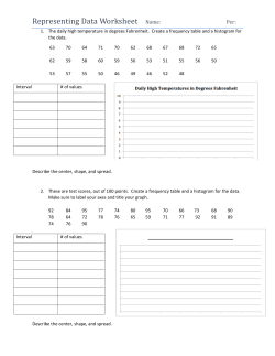


© Copyright 2026