1. shopping
2. resources
3. loyalty programs

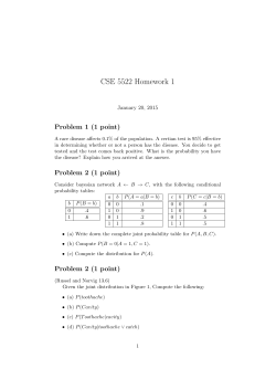
Dynamics Analytics for Spatial Data with an
Incremental Clustering Approach
Fernando Mendes, Maribel Yasmina Santos
João Moura-Pires
ALGORITMI Research Centre
University of Minho
Guimarães, Portugal
[email protected], [email protected]
CENTRIA, Faculty of Science and Technology
New University of Lisbon
Lisbon, Portugal
[email protected]
Abstract— Several clustering algorithms have been extensively
used to analyze vast amounts of spatial data. One of these
algorithms is the SNN (Shared Nearest Neighbor), a densitybased algorithm, which has several advantages when analyzing
this type of data due to its ability of identifying clusters of
different shapes, sizes and densities, as well as the capability to
deal with noise. Having into account that data are usually
progressively collected as time passes, incremental clustering
approaches are required when there is the need to update the
clustering results as new data become available. This paper
proposes SNN++, an incremental clustering algorithm based on
the SNN. Its performance and the quality of the resulting
clusters are compared with the SNN and the results show that
the SNN++ yields the same result as the SNN and show that the
incremental feature was added to the SNN without any
computational penalty. Moreover, the experimental results also
show that processing huge amounts of data using increments
considerably decreases the number of distances that need to be
computed to identify the points’ nearest neighbors.
Keywords-clustering; incremental clustering; shared nearest
neighbor; spatial data
I.
INTRODUCTION
Nowadays, huge amounts of data are collected making
use of a variety of devices like satellite images, medical
equipment,
geographical
information
systems,
telecommunication devices, sensor technologies, among
many others. Data Mining and in particular cluster analysis
can help to automate the analysis of such vast amount of data
and identify patterns present in data [1].
Clustering is the process of grouping large datasets where
objects in the same group should be as similar as possible
and different to objects in other groups. It is known as
unsupervised learning as no a priori information about the
data is required [2]. Clusters emerge naturally from the data
under analysis using some distance function to measure the
similarity among objects. This technique is classified in four
main categories [1, 3]: Partition Clustering, Hierarchical
Clustering, Density-based Clustering and Grid-based
Clustering.
In this paper Density-based algorithms, and namely the
SNN (Shared Nearest Neighbor) algorithm, are the focus of
this work due to the fact that this type of clustering presents
several advantages when analyzing spatial data, one of the
domains where vast amounts of data are collected every day
[3].
Density-based algorithms identify clusters independently
of their shape or size. Typically, they classify dense regions
as clusters and classify as noise, regions with low density of
objects.
The SNN algorithm presents as main advantages the
capability to identify clusters of different shapes, sizes and
densities, as well as the capability to deal with noise [4].
In most applications the data are progressively collected
as time passes. Incremental clustering approaches are
beneficial when there is the need to update the clustering
results as new data become available.
Several incremental clustering algorithms have been
proposed, ranging from partitioning to density-based, for
instance, in the partitioning category, the Incremental Kmeans [5] and in the density-based category, the
IncrementalDBSCAN [6].
Regarding SNN, few works address this algorithm in an
incremental way. To the best of our knowledge, only a poster
was recently published [7] but with few details about the
followed strategy and with a performance evaluation with
small dataset.
The SNN algorithm starts with the identification of the knearest neighbors of a point, being this step the responsible
for the time complexity of the algorithm. This paper
proposes an incremental approach to SNN, named SNN++,
that is able to add new data points to the available clusters
without the need to re-compute all the k-nearest neighbors.
This approach provides the same results as the SNN
algorithm, ensuring the quality of the produced output, and is
able to process bulks of data as they become available. The
incremental processing of data is crucial in a context where
data are collected in a continuous way and the clustering
results can be updated as new increments are ready to be
processed. This avoids the need to store huge amounts of
data, to be processed later and, also, decreases the clustering
duration, as the time needed to process an increment is
substantially lower than the time needed to compute all the
data set. In both clustering approaches, SNN and SNN++, the
identification of the nearest neighbors of a point represents
the most time consuming step. An incremental clustering
approach reduces the impact of this step, as less data are
processed in each increment. This paper introduces the
SNN++ and shows the impact of an incremental clustering
approach.
The rest of this paper is organized as follows. Section II
presents related work. Section III summarizes the approach
followed by the SNN algorithm to cluster a data set. Section
IV describes the SNN++ algorithm proposed in this paper.
Section V shows the results obtained with the use of SNN++
in synthetic and real data sets. Section VI summarizes the
main findings of this work and presents some guidelines for
future work.
AffectedD(p)
p
NEps(p)
Figure 1. Affected objects in a sample database [6].
II. RELATED WORK
Incremental clustering is a recent area of research with
increasing interest from the research community due to the
ever increasing size of data sets and the need to incorporate
database updates without having to mine the entire data
again [3]. Several incremental approaches have been
proposed so far like IncrementalDBSCAN [6] and
Incremental K-means [5].
Incremental K-Means uses the original K-Means to
execute the clustering process on the initial data. When new
data are available, Incremental K-Means measures the new
cluster centers by calculating the mean value of the objects
present in a cluster without rerunning the algorithm. The
authors claim that the algorithm provides better and faster
results compared to the existing K-Means algorithm if the
changes to the original database don not exceed a certain
amount.
Although some other incremental clustering approaches
can be found in the literature, next paragraphs will focus on
density based ones, namely in those that address the
DBSCAN algorithm, due to the similarity between
DBSCAN and SNN. Both algorithms share the same
advantages, but SNN is able to detect clusters of different
densities, one of the main drawbacks of DBSCAN.
In [6] the first incremental version of DBSCAN, called
IncrementalDBSCAN, was proposed. The main principle of
this incremental approach is that on insertion or on deletion
of an object p, the set of affected objects is the set of objects
in the neighborhood of p with a given radius Eps, NEps(p),
and all objects that are density reachable from p or from one
of its neighbors (Figure 1). The affected objects may change
clusters’ membership after an update or a delete operation.
All the remaining objects, outside the affected area, will not
change cluster membership. In the DBSCAN algorithm, the
Eps parameter represents the radius that limits the
neighborhood area of an object, while MinPts represents the
minimum number of objects that must exist in the Epsneighborhood of an object to form a cluster.
The insertion of a new point can result in the
identification of noise, the creation of a new cluster, the
absorption of the new point by existing clusters or in a
merging of existing clusters (Figure 2).
When deleting an object, established connections
between objects are removed but no new connections are
established. The existing clusters may be removed, reduced
or split.
p
Noise
p
Absorption
p
Creation
p
Merge
Figure 2. Different cases for insertion of new points [6].
In [2], the authors propose a more efficient incremental
algorithm than IncrementalDBSCAN, which allows adding
points in a bulk process as opposed to one data point at a
time. This approach uses DBSCAN to cluster the new data
and merges the resulting clusters with the previous ones. The
new data points that are present in the intersection of the old
and new datasets are added using the IncrementalDBSCAN
algorithm.
The authors in [8] use a grid density based clustering
algorithm (GDCA) that can discover clusters with arbitrary
shapes and sizes. The algorithm first partitions the data space
into units and then applies the DBSCAN algorithm to these
units instead of points. Only the units that have a density of
at least a given density threshold are useful in extending
clusters. The same authors also proposed an incremental
clustering algorithm (IGDCA), based on GDCA, which
handles bulk of updates [8].
Recently, an incremental version of the SNN algorithm
was proposed [7]. Although no details about the proposed
implementation are given, the authors mention that their
approach has as main disadvantage a high memory usage
when compared with the SNN. Moreover, the authors only
present performance evaluations for 5000 insertions of new
points, a value that does not allow any comparison with the
version proposed in this paper, which results are presented
afterwards in section V.
III. THE SHARED NEAREST NEIGHBOR ALGORITHM
The Shared Nearest Neighbor (SNN) [4] is a densitybased clustering algorithm that is suitable for finding clusters
of arbitrary shapes and densities, handling outliers and noise.
Furthermore, there is no need to give the number of clusters
as parameter [4]. The notion of similarity in the SNN
algorithm is based on the number of neighbors that two
points share, value that is computed after the identification of
the k-nearest neighbors of each point [9]. The nearest
neighbors are identified adopting a distance function. In
spatial data, the distance function usually includes the
Euclidean distance or the Geographical distance. The
distance function that is used to measure the similarity
between objects can be extended in order to integrate in the
clustering process several dimensions of analysis [10].
The SNN algorithm includes three input parameters: k,
the number of nearest neighbors that must be identified for
each point; Eps, the density threshold that establish the
minimum number of neighbors two points should share to be
considered close to each other; and, MinPts, the minimum
density that a point should have to be considered a core
point. Clusters are defined using the found core points.
This algorithm includes several steps [9], namely:
1. Create the distance matrix using a given distance
function and identify for each point, the k nearest neighbors.
3. For each two points, calculate the similarity, which is
given by the number of shared neighbors.
4. Establish the SNN density of each point. The SNN
density is given by the number of nearest neighbors that
share Eps or more neighbors.
5. Identify the core points of the data set. Each point that
has a SNN density greater or equal to MinPts is considered a
core point.
6. Build clusters from core points. Two core points are
allocated to the same cluster if they share Eps or more
neighbors with each other.
7. Handle noise points. Points not classified as core
points and that are not within Eps of a core point are
considered noise.
8. Assign the remaining points to clusters. All non-core
and non-noise points are assigned to the nearest cluster.
To show how the algorithm works, a synthetic data set
with 322 points will be used as demonstration case. The
SNN parameters used on this dataset were k=7, Eps=2,
MinPts=5.
The first step of the algorithm is to create the distance
matrix and identify the k nearest neighbors. Figure 3 shows
the links between the k-neighbors of all points. The next step
is to calculate the shared nearest neighbors between pairs of
points and to establish the SNN density of each point. The
SNN density is given by the number of nearest neighbors
that share Eps or more neighbors. Figure 4 shows all points
that have a SNN density greater than Eps connected with a
line. All points with a SNN density of MinPts or greater are
identified as core points. All core points that share Eps or
more neighbors are allocated to the same cluster and
continue to be core points. All non-core points that share Eps
or more neighbors are also included in the same cluster but
are classified as border points of that cluster. All the
remaining points not integrated in a cluster are classified as
noise points. Figure 5 shows the result of the SNN algorithm
with the 7 identified clusters.
Figure 3. Connection graph of the k-neighbours list
Figure 4. SNN-Density connection graph
Figure 5. Result of SNN with k=7, Eps=2, MinPts=5
The process of looking for the k nearest neighbors of a
point requires the comparison of a point with all the others in
the data set, reason why the time complexity of SNN is O(n2)
[9]. In low dimensional data sets the expected time
complexity is n*log(n) using a metric data structure like a
kd-tree [11]. Although complexity and as consequence the
time needed to process data can be reduced, the processing
of new data in an incremental way avoids the reprocessing of
already clustered data. By this way the existent clusters can
be updated with new data in an iterative way.
IV.
THE SNN++ APPROACH
The proposed algorithm, the SNN++, is based on the SNN
[4] maintaining its capabilities of identifying clusters of
arbitrary shapes, sizes and densities, as well as handling
noise.
SNN++ uses the same 3 input parameters: k, Eps and
MinPts. In a general description, the algorithm executes the
clustering of the initial data set using the SNN. From this
step forward, SNN++ receives new data that are added to the
existing clusters without the need to restart all the process.
The clusters are updated each time new data arrives. In this
process, new clusters can emerge or be split as consequence
of the new densities.
The SNN++ algorithm will be detailed described
afterwards. For now consider an example in which the first
iteration, with all the available data (67 points), produced the
SNN density shown in Figure 6. The SNN parameters used
were k=7, Eps=2 and MinPts=5. Although there seems to
exist 2 clusters, the algorithm only found 1 for now. The data
point A in Figure 6 has a SNN density of 6 and is therefore a
core point, since MinPts=5. This means that all shared
neighbors of this point that share Eps or more neighbors
belong to its cluster. This happens with the 3 neighbors (B, C
and D) represented in Figure 6.
When new data arrives, in this example more 44 points,
the SNN++ creates the k-nearest neighbors list only for these
new points and measures the densities of all objects (the
initially clustered and the new ones). The affected points are
all new points and the existing points that saw their list of
reflexives points (a list with all shared neighbors that share
Eps or more neighbors) changed. In this example all the
points from A to F are affected (Figure 7). There are now 2
clusters found by the algorithm as shown in Figure 7. The
Point A saw its SNN density reduced to 3 in comparison to
the previous iteration. Because of this it is no longer a core
point and therefore the points in its reflexive list no longer
have to be in the same cluster as itself. Only clusters with
affected objects can change from one iteration to another. All
other clusters remain the same and do not need to be rebuilt.
Figure 6. SNN Density Graph of the Initial dataset (k=7, Eps=2 and
MinPts=5)
Figure 7. SNN Density Graph after adding new data (k=7, Eps=2 and
MinPts=5)
Next follows a detailed description of the proposed
algorithm.
The SNN++ starts by reading an initial dataset and applies
the SNN clustering process on them. After this the
incremental clustering process initiates and for each new
dataset the following steps are executed:
1. Read incremental dataset
2. Calculate the k-nearest neighbors of each new object
3. Measure the similarities and the densities of all
objects and identify the objects affected by the newly
added data objects
4. Build clusters starting with the core points of the
affected data objects identified in the previous step
5. Identify border points and noise points by iterating
through the remaining points of the affected objects
For each new dataset steps 1 to 5 are repeated. A dataset
with the new data is read and for each new object the knearest neighbors are computed (Algorithm 1). The
computation of the k-nearest neighbor list requires the
calculation of the distance between all objects using a given
distance function. The SNN++ does not need to recalculate
the distance between existing data points, as it uses the knearest neighbor lists already computed in the previous
iteration. In the same step (Algorithm 1), the algorithm
updates the k-nearest neighbor list of all objects by adding
the new points to the k-nearest neighbor list in case these
new points have smaller distance values than the existing
ones.
The next step is to measure the similarities and densities
of all objects (Algorithm 2). If two objects are mutual
neighbors and this number is greater or equal than Eps, both
objects are added to each other’s list of reflexives. In the
same step (Algorithm 2), the algorithm adds all objects to the
list of affected objects that saw their list of reflexives
changed since the previous iteration, including all newly
added objects. The list of affected objects contains all objects
that are affected by the new data added on the current
iteration. If there are core points in the list of affected
objects, clusters are formed around them (Algorithm 3).
The last step (Algorithm 4), takes the remaining objects from
the list of affected objects and identifies all border points and
assigns them to the formed clusters.
Algorithm (1) Step 6: Obtain the k-nearest neighbors of each new
object
1: for all objects o in arraylist NewData do
2: knn-list = get k-nearest neighbors(o)
3: for all objects p in arraylist OldData do
4:
update p(neighbor list)
5: end for
6: end for
Algorithm (2) Step 7: Measure the similarities and the densities of
all objects and identify the objects affected by the new objects
1: for all objects o in arraylist DataSet do
2: empty o (reflexive list)
3: knn-list = k-nearest neighbors (o)
4: for all objects p in knn-list do
5:
if p and o are mutual neighbors then
6:
measure the similarity between them
7:
if similarity >= Eps then
8:
add p to o(reflexive list)
9:
end if
10:
end if
11: end for
12: if o(reflexive list) changed from previous iteration then
13:
add o to list AffectedObjects
14: end if
15: if size of o(reflexive list) >= MinPts then
16:
define the o as Core
17: else
18:
define o as noise
19:
define o as belonging to no cluster
20: end if
21: end for
Algorithm (3) Step 8: Build clusters starting with the
representative objects of the affected data points identified in the
previous step
1: for all objects o in list AffectedObjects do
2: if o does not belong to a cluster and o is Core do
3:
assign o to new cluster cl
4:
add o to new arraylist li
6:
for all objects p from arraylist li do
7:
add p to cluster cl
8:
if p is noise then
9:
define p as border
10:
else if p is core then
11:
add all objects contained in p (reflexive list) to arraylist li
12:
end if
13:
end for
14: else if o belongs to a cluster do
15:
remove o from list AffectedObjects
16: end if
17: end for
As already mentioned, the SNN temporal complexity
is O(n2), as the identification of the k-nearest neighbors
requires the calculation of the distances among all the points
in the data set. For the SNN++, and taking into consideration
that a data set of length n will be processed in m increments
of length n/m, the processing of increment i requires the
identification of the distances between the new
points, (n/m) 2, and the distances between theses points and
the previously processed ones, (n/m)*(i-1)*(n/m). After
processing all increments, the number of distance
computations is represented by ((1+1/m)/2)*n2, which means
that the complexity of the SNN++ remains O(n2).
Algorithm (4) Step 9: Identify border points and noise points by
iterating through the remaining points of the affected objects
1: for all objects o in list AffectedObjects do
2: for all points p in o(reflexive list) do
3:
if (p is core) and (p is not in the same cluster as o) then
4:
add o to the same cluster as p
5:
define o as border
6:
break (leave for cycle)
7:
end if
8: end for
9: end for
V. RESULTS
This section presents the experimental results that are
performed to evaluate the quality and the performance of the
SNN++. Quality is tested using a synthetic dataset, the t5.8k
from CHAMELEON [12], and performance is tested using a
real dataset. In this case, the SNN is also used to verify the
obtained gain when using an incremental approach. The real
dataset is named the MARIN dataset, which integrates
tracking data of shipping movements collected by the
Netherlands Coastguard [10].
A deliberate decision was made to not compare the
SNN++ performance with other algorithms, besides the SNN,
as it would not be a fair comparison because of the
differences in the implementations. The SNN++ and SNN on
the other hand share a huge portion of code assuring a just
comparison between the two.
A. Quality Evaluation
The dataset t5.8k is used to evaluate the quality of the
SNN++ algorithm, integrating 8000 points as shown in Figure
8. The t5.8k was split in 6 smaller datasets, each one
containing one letter of approximately 1300 points. These
datasets were added one by one, in an iterative process, to
the SNN++ until the original t5.8k dataset was rebuilt. The
sequence in which the letters were added was G, E, O, R, G
and E.
The clustering result was compared with the result
obtained with the SNN using for both the following
parameters: k=46, Eps=15 and MinPts=43. The values for
these parameters were obtained from [13] in which the
authors propose a method for estimating these parameters.
Figure 8. t5.8k dataset with 8000 points
Figure 9 shows the results of SNN++. Each image is
associated with one iteration, starting with one letter and
ending with the 6. The last image shows the final clustering
result of the incremental algorithm. A detailed analysis of
both SNN++ and SNN results allowed the verification of a
correspondence of 100% in the obtained clusters.
for SNN and SNN++, for a subset of 200,000 points, are
compared for an incremental step of 20,000 points. Looking
at the value for 160,000 points, as an example, the runtime
required by the SNN to process all the 160,000 points (in just
one bulk of data) is slightly higher than the runtime required
by the SNN++ to process all the 160,000 points (using
incremental additions of 20,000 points). In fact, in all
executed experiments, the SNN++ presents a computational
pattern almost equivalent or slightly better than the SNN.
These experiments provide empirical evidence that the
incremental characteristic of SNN++ was introduced in SNN
without any computational penalty. If the data arrive in an
incremental way of n/m data points per increment, the
number of distances that needs to be computed in the last
increment is n2/m, which represents, possibly, a very small
fragment of n2. For instance, looking at Figure 11, the time
required by the SNN++ to process the last (10th) data
increment of 20,000 points is around 19% of the time
required by the SNN to compute all the data set of 200,000
points.
6000000"
SNN++'
B. Performance Evaluation
The data set used to evaluate the performance of SNN++
was the MARIN data set, integrating 280,000 data points
(Figure 10).
Figure 10. MARIN dataset with 280 000 data points
To compare the performance of SNN and SNN++, various
experiments were carried out based on MARIN data set, with
different incremental steps ranging from 10,000 points to
70,000 points. In the graphic shown in Figure 11, the runtime
3000000"
2000000"
1000000"
2000
00"
1800
00"
1600
00"
1400
00"
1200
00"
1000
00"
8000
0"
6000
0"
0"
4000
0"
This quality assessment had as objective to show that
both approaches, incremental or not, produce the same
results. Another experiment performed was to split the
dataset randomly in 6 smaller ones. As expected, the
clustering results after each one of the first five iterations
were not so good. However, the final iteration returned the
same result as the SNN approach.
SNN'
4000000"
2000
0"
Figure 9. Results of SNN++ on t5.8k dataset, noise discarded
Run$me'in'ms'
5000000"
Points'
Figure 11. Comparison of runtime between SNN and SNN++
The computational effort that SNN++ needs to compute
new data points depends on the number of points that were
processed in previous increments.
Taking into consideration that to process n points
in m increments of n/m points each, increment i requires an
additional computation of i*(n/m)2 distances, the effort to
compute a new bulk increases as the number of points
already processed also increases. However, and as presented
in Algorithm (3), the time needed to rebuild the clusters also
needs to be considered. Figure 12 shows the average time,
per processed point, of the total time and, also, of each one
of the main components, as the computation of distances and
the rebuilt of clusters for increments of 10,000 points. As it
can be seen, the average time per point increases as the
number of already processed points also increases, either in
the computation of distances and in the clusters rebuilt.
For the same experiment presented in Figure 12, Figure
13 shows the relative importance, in terms of processing
time, of the main algorithmic components.
50"
Increments
of 10K
45"
40"
35"
30"
ms
Distance"
25"
Cluster"
20"
Total"
15"
10"
5"
0"
0"
50000"
100000"
150000"
200000"
Points
Figure 12. Average processing time per new point in SNN++ with increments
of 10,000 points
100%$
Increments
of 10K
98%$
96%$
94%$
ACKNOWLEDGMENT
Other$
92%$
90%$
Wri4ng$
88%$
Reflex$List$
86%$
Cluster$
84%$
Distance$
10000$
20000$
30000$
40000$
50000$
60000$
70000$
80000$
90000$
100000$
110000$
120000$
130000$
140000$
150000$
160000$
170000$
180000$
190000$
200000$
82%$
80%$
The algorithm was tested in what concerns quality and
performance. The quality was measured running the
algorithm on a synthetic dataset and comparing the clustering
results with the ones obtained with SNN. The same testing
environment and the same input parameters were used for
both incremental and non-incremental approach. Both
approaches produced the same results.
The performance was tested using a dataset with real data
and the results were also compared with the SNN. The
results show that the incremental feature was added to SNN
without any computational penalty. Moreover, the
experimental results show that processing huge amounts of
data using increments considerably decreases the number of
distances that need to be computed to identify the points’
nearest neighbors
As future work, the SNN++ will address improvements in
the identification of the nearest neighbors’ list as well as the
identification of relevant changes in the clusters constitution
from one iteration to another.
The implementation of the SNN and SNN++ used in this
work will be available in JAVA as open-source code.
Points
This work was partly funded by FEDER funds through
the Operational Competitiveness Program (COMPETE), by
FCT with the project: FCOMP-01-0124-FEDER-022674 and
by Novabase Business Solutions with a co-funded QREN
project (24822).
We would like to thank the Maritime Research Institute
in the Netherlands, for making the data available for analysis
under the MOVE EU Cost Action IC0903 (Knowledge
Discovery from Moving Objects).
Figure 13. Runtime distribution of the main components from SNN++ with
increments of 10,000 points
As it can be observed, as the number of already
processed points grows, the rebuild of clusters becomes more
important but the distance computation remains, clearly, the
most important component. These data were collected for the
experiments with the MARIN data set with increments
ranging from 10,000 points to 70,000 points and the
empirical observations remain valid. In this range, the time
needed to process the 200,000 points remains almost the
same. With smaller increments, ranging from 100 points to
1,000 points, the time to process the 200,000 points is clearly
higher. Although this observation is limited to this particular
data set, the SNN++ performance seems to remain constant to
a wide range of the increment size.
VI.
CONCLUSIONS AND FUTURE WORK
This paper presented an incremental clustering algorithm,
the SNN++, based on the SNN algorithm. The SNN++
maintains the capabilities of the SNN with the advantage of
being able to process new data, integrating these new data in
the existing clusters, without the need to re-compute the
entire nearest neighbors list and, as consequence, repeat the
whole clustering process.
REFERENCES
[1]
[2]
[3]
[4]
[5]
[6]
[7]
[8]
[9]
M. Halkidi, Y. Batistakis, and M. Vazirgiannis, "On clustering
validation techniques," Journal of Intelligent Information Systems,
vol. 17, pp. 107--145, 2001.
N. a. G. Goyal, P. and Venkatramaiah, K. and PS, S., "An Efficient
Density Based Incremental Clustering Algorithm in Data
Warehousing Environment," in 2009 International Conference on
Computer Engineering and Applications, 2011.
J. Han, M. Kamber, and J. Pei, Data mining: concepts and
techniques, 3 ed.: Morgan Kaufmann, 2011.
L. Ertöz, M. Steinbach, and V. Kumar, "A new shared nearest
neighbor clustering algorithm and its applications," presented at the
Workshop on Clustering High Dimensional Data and its Applications
at 2nd SIAM International Conference on Data Mining, 2002.
S. Chakraborty and N. Nagwani, "Analysis and Study of Incremental
K-Means Clustering Algorithm," in High Performance Architecture
and Grid Computing, ed: Springer, 2011, pp. 338--341.
M. Ester, H. P. Kriegel, J. Sander, M. Wimmer, and X. Xu,
"Incremental clustering for mining in a data warehousing
environment," presented at the Proceedings of the International
Conference on Very Large Data Bases, 1998.
S. Singh and A. Awekar, "Incremental Shared Nearest Neighbor
Density Based Clustering," 1st Indian Workshop on Machine
Learning, 2013.
N. Chen, A. Chen, and L. Zhou, "An incremental grid density-based
clustering algorithm," Journal of software, vol. 13, pp. 1--7, 2002.
L. Ertöz, M. Steinbach, and V. Kumar, "Finding clusters of different
sizes, shapes, and densities in noisy, high dimensional data,"
presented at the SIAM international conference on data mining, 2003.
[10]
[11]
M. Y. Santos, J. P. Silva, J. Moura-Pires, and M. Wachowicz,
Automated Traffic Route Identification Through the Shared Nearest
Neighbour Algorithm: Springer Berlin Heidelberg, 2012.
J. H. Friedman, J. L. Bentley, and R. A. Finkel, "An algorithm for
finding best matches in logarithmic expected time," ACM
Transactions on Mathematical Software (TOMS), vol. 3, pp. 209-226, 1977.
[12]
[13]
G. Karypis, E.-H. Han, and V. Kumar, "Chameleon: Hierarchical
clustering using dynamic modeling," Computer, vol. 32, pp. 68--75,
1999.
G. Moreira, M. Y. Santos, and J. Moura-pires, "SNN Input
Parameters: how are they related  ?," to be presented at the Crowd and
Cloud Computing Workshop at International Conference on Parallel
and Distributed Systems, 2013.