1. No category

5. ANALYSIS OF WAVESHAPE
5
Analysis of Waveshape and Waveform Complexity
Some biomedical signals, e.g., the ECG and carotid pulse,
have simple and recognizable waveshapes, which are
modified by abnormal events and pathological processes.
–697–
c R.M. Rangayyan, IEEE/Wiley
5. ANALYSIS OF WAVESHAPE
EMG, PCG, VAG: no identifiable waveshapes.
EMG: complex interference patterns of several SMUAPs.
PCG: vibration waves with no specific waveshapes.
The waveform complexity in the EMG and the PCG varies
in relation to physiological and pathological phenomena.
Analyzing the waveform complexity of such signals may
assist in understanding of the processes they reflect.
–698–
c R.M. Rangayyan, IEEE/Wiley
5. ANALYSIS OF WAVESHAPE
5.1
5.1. PROBLEM STATEMENT
Problem Statement
Explain how waveshapes and waveform complexity
in biomedical signals relate to the characteristics
of the underlying physiological and
pathological phenomena.
Propose techniques to parameterize and analyze
the signal features you identify.
–699–
c R.M. Rangayyan, IEEE/Wiley
5. ANALYSIS OF WAVESHAPE
5.2
5.2. ILLUSTRATION OF THE PROBLEM WITH CASE-STUDIES
Illustration of the Problem with Case-studies
5.2.1 The QRS complex in the case of bundle-branch block
The His bundle and its branches conduct the
cardiac excitation pulse from the AV node to the ventricles.
A block in one of the bundle branches causes asynchrony
between the contraction of the left and the right ventricles.
–700–
c R.M. Rangayyan, IEEE/Wiley
5. ANALYSIS OF WAVESHAPE
5.2. ILLUSTRATION OF THE PROBLEM WITH CASE-STUDIES
This causes a staggered summation of the action potentials
of the myocytes of the left and the right ventricles
over a longer-than-normal duration.
The result is a longer and possibly jagged QRS complex.
–701–
c R.M. Rangayyan, IEEE/Wiley
5. ANALYSIS OF WAVESHAPE
5.2. ILLUSTRATION OF THE PROBLEM WITH CASE-STUDIES
5.2.2 The effect of myocardial ischemia and infarction on QRS
waveshape
Occlusion of a coronary artery or a branch due to
deposition of fat, calcium, etc. results in reduced
blood supply to a portion of the cardiac musculature:
the part of the myocardium served by the affected artery
suffers from ischemia — lack of blood supply.
–702–
c R.M. Rangayyan, IEEE/Wiley
5. ANALYSIS OF WAVESHAPE
5.2. ILLUSTRATION OF THE PROBLEM WITH CASE-STUDIES
Prolonged ischemia leads to myocardial infarction:
the deceased myocytes cannot contract any more,
and no longer produce action potentials.
Action potential of an under-nourished ventricular myocyte:
smaller amplitude and shorter duration.
ST segment either elevated or depressed,
T wave may be inverted.
–703–
c R.M. Rangayyan, IEEE/Wiley
5. ANALYSIS OF WAVESHAPE
5.2. ILLUSTRATION OF THE PROBLEM WITH CASE-STUDIES
5.2.3 Ectopic beats
Ectopic beats generated by cardiac tissue that possess
abnormal pacing capabilities.
Ectopic beats originating in the atria: altered P waveshape
due to different paths of propagation of the excitation pulse.
QRS complex of atrial ectopic beats will appear normal.
–704–
c R.M. Rangayyan, IEEE/Wiley
5. ANALYSIS OF WAVESHAPE
5.2. ILLUSTRATION OF THE PROBLEM WITH CASE-STUDIES
Ectopic beats originating on the ventricles (PVCs):
bizarre waveshapes due to differing paths of conduction.
PVCs typically lack a preceding P wave.
PVCs triggered by ectopic foci close to the AV node
may possess near-normal QRS shape.
RR intervals of preceding beat (short) and
succeeding beat (compensatory pause) play important
roles in determining the nature of ectopic beats.
–705–
c R.M. Rangayyan, IEEE/Wiley
5. ANALYSIS OF WAVESHAPE
5.2. ILLUSTRATION OF THE PROBLEM WITH CASE-STUDIES
5.2.4 EMG interference pattern complexity
Motor units are recruited by two mechanisms —
spatial and temporal recruitment — to produce
increasing levels of contraction and muscular force output.
SMUAPs of the active motor units overlap and produce a
complex interference pattern.
Increasing complexity of EMG with
increasing level of contraction.
–706–
c R.M. Rangayyan, IEEE/Wiley
5. ANALYSIS OF WAVESHAPE
5.2. ILLUSTRATION OF THE PROBLEM WITH CASE-STUDIES
5.2.5 PCG intensity patterns
Vibration waves in PCG not amenable to visual analysis.
General intensity pattern of PCG over a cardiac cycle
recognizable by auscultation or visual inspection.
Cardiovascular diseases and defects alter the
relative intensity patterns of S1 and S2,
cause additional sounds or murmurs,
split S2 into two distinct components, etc.
–707–
c R.M. Rangayyan, IEEE/Wiley
5. ANALYSIS OF WAVESHAPE
5.2. ILLUSTRATION OF THE PROBLEM WITH CASE-STUDIES
Many diseases may cause systolic murmurs;
intensity pattern or envelope of murmur could assist
in arriving at a specific diagnosis.
–708–
c R.M. Rangayyan, IEEE/Wiley
5. ANALYSIS OF WAVESHAPE
5.3
5.3. ANALYSIS OF EVENT-RELATED POTENTIALS
Analysis of Event-related Potentials
Most important parameter in a visual ERP:
timing or latency of the first major positivity P120.
Latencies of the troughs before and after P120,
called N80 and N145, are also of interest.
Amplitudes of ERP features of lesser importance.
–709–
c R.M. Rangayyan, IEEE/Wiley
5. ANALYSIS OF WAVESHAPE
5.4
5.4. MORPHOLOGICAL ANALYSIS OF ECG WAVES
Morphological Analysis of ECG Waves
ECG waveshape changed by many abnormalities:
myocardial ischemia or infarction,
bundle-branch block, and ectopic beats.
–710–
c R.M. Rangayyan, IEEE/Wiley
5. ANALYSIS OF WAVESHAPE
5.4. MORPHOLOGICAL ANALYSIS OF ECG WAVES
5.4.1 Correlation coefficient
Problem: Propose a general index
to indicate altered QRS waveshape.
You are given a normal QRS template.
–711–
c R.M. Rangayyan, IEEE/Wiley
5. ANALYSIS OF WAVESHAPE
5.4. MORPHOLOGICAL ANALYSIS OF ECG WAVES
Solution: Jenkins et al. used correlation coefficient
γxy =
"
P
N −1
n=0
P
N −1
n=0
x(n) y(n)
x2(n)
P
N −1
n=0
#
y 2(n)
1/2
.
Normal beat used as template to compute γxy
for each detected beat; see Figure 2.2.
Most normal beats: γxy > 0.9.
PVCs and beats with abnormal shape: lower values of γxy .
–712–
c R.M. Rangayyan, IEEE/Wiley
5. ANALYSIS OF WAVESHAPE
5.4. MORPHOLOGICAL ANALYSIS OF ECG WAVES
5.4.2 The minimum-phase correspondent and signal length
Most of the energy of a normal ECG signal is concentrated
within an interval of about 80 ms in the QRS complex.
Normally iso-electric PQ, ST, and TP segments: no energy.
Certain abnormal conditions cause the QRS to widen
or the ST segment to bear a nonzero value:
energy of signal spread over a longer duration.
–713–
c R.M. Rangayyan, IEEE/Wiley
5. ANALYSIS OF WAVESHAPE
5.4. MORPHOLOGICAL ANALYSIS OF ECG WAVES
Problem: Investigate the effect of the
distribution of energy over the time axis
on a signal’s characteristics.
Propose measures to parameterize the effects and
study their use in the classification of ECG beats.
–714–
c R.M. Rangayyan, IEEE/Wiley
5. ANALYSIS OF WAVESHAPE
5.4. MORPHOLOGICAL ANALYSIS OF ECG WAVES
Solution:
Signal x(t): distribution of the amplitude
of a certain variable over the time axis.
x2(t): instantaneous energy of the signal.
x2(t), 0 ≤ t ≤ T : energy distribution or density function.
Total energy of the signal:
Ex =
T
0
Z
x2(t) dt.
–715–
(5.1)
c R.M. Rangayyan, IEEE/Wiley
5. ANALYSIS OF WAVESHAPE
5.4. MORPHOLOGICAL ANALYSIS OF ECG WAVES
Facilitates definition of moments of the energy distribution.
Centroidal time:
tx̄ =
T
0
RT
0
R
t x2(t) dt
.
2
x (t) dt
(5.2)
Dispersion of energy about the centroidal time:
σt2x̄ =
T
0
R
(t − tx̄)2 x2(t) dt
.
RT
2
0 x (t) dt
–716–
(5.3)
c R.M. Rangayyan, IEEE/Wiley
5. ANALYSIS OF WAVESHAPE
5.4. MORPHOLOGICAL ANALYSIS OF ECG WAVES
Similarity between the equations above and
Equations 3.1 and 3.3: normalized function
px(t) =
T
0
R
x2(t)
x2(t) dt
(5.4)
treated as a PDF.
Other moments may also be defined to characterize and
study the distribution of x2(t) over the time axis.
–717–
c R.M. Rangayyan, IEEE/Wiley
5. ANALYSIS OF WAVESHAPE
5.4. MORPHOLOGICAL ANALYSIS OF ECG WAVES
Minimum-phase signals:
Distribution of energy of a signal over its duration
related to its amplitude spectrum and phase spectrum.
Notion of minimum phase useful in analyzing
the distribution of energy over the time axis.
–718–
c R.M. Rangayyan, IEEE/Wiley
5. ANALYSIS OF WAVESHAPE
5.4. MORPHOLOGICAL ANALYSIS OF ECG WAVES
A signal x(n) is a minimum-phase signal if both the signal
and its inverse xi(n) are one-sided signals —
completely causal or anti-causal — with finite energy:
∞
X
x2(n) < ∞,
∞
X
x2i (n) < ∞.
n=0
n=0
Note: The inverse of a signal is defined such that
x(n) ∗ xi(n) = δ(n); equivalently, Xi(z) =
–719–
1
X(z) .
c R.M. Rangayyan, IEEE/Wiley
5. ANALYSIS OF WAVESHAPE
5.4. MORPHOLOGICAL ANALYSIS OF ECG WAVES
Important properties of a minimum-phase signal:
For a given amplitude spectrum,
there exists one and only one minimum-phase signal.
–720–
c R.M. Rangayyan, IEEE/Wiley
5. ANALYSIS OF WAVESHAPE
5.4. MORPHOLOGICAL ANALYSIS OF ECG WAVES
Of all finite-energy, one-sided signals
with identical amplitude spectra,
the energy of the minimum-phase signal is
optimally concentrated toward the origin,
and the signal has the smallest phase lag
and phase-lag derivative at each frequency.
–721–
c R.M. Rangayyan, IEEE/Wiley
5. ANALYSIS OF WAVESHAPE
5.4. MORPHOLOGICAL ANALYSIS OF ECG WAVES
The z -transform of a minimum-phase signal has
all poles and zeros inside the unit circle in the z -plane.
The complex cepstrum of a minimum-phase signal
is causal.
–722–
c R.M. Rangayyan, IEEE/Wiley
5. ANALYSIS OF WAVESHAPE
5.4. MORPHOLOGICAL ANALYSIS OF ECG WAVES
Minimum-phase and maximum-phase components:
A signal x(n) that does not satisfy
the minimum-phase condition,
referred to as a composite signal or a mixed-phase signal,
may be split into its minimum-phase component
and maximum-phase component
by filtering its complex cepstrum x̂(n).
–723–
c R.M. Rangayyan, IEEE/Wiley
5. ANALYSIS OF WAVESHAPE
5.4. MORPHOLOGICAL ANALYSIS OF ECG WAVES
To obtain the minimum-phase component,
the causal part of the complex cepstrum is chosen as:












0
n<0
x̂min(n) =  0.5 x̂(n) n = 0 .






 x̂(n)
n>0
(5.5)
The inverse procedures yield the
minimum-phase component xmin(n).
–724–
c R.M. Rangayyan, IEEE/Wiley
5. ANALYSIS OF WAVESHAPE
5.4. MORPHOLOGICAL ANALYSIS OF ECG WAVES
Maximum-phase component obtained by application of the
inverse procedures to the anti-causal part of the cepstrum:












x̂(n)
n<0
x̂max(n) =  0.5 x̂(n) n = 0 .






 0
n>0
–725–
(5.6)
c R.M. Rangayyan, IEEE/Wiley
5. ANALYSIS OF WAVESHAPE
5.4. MORPHOLOGICAL ANALYSIS OF ECG WAVES
The minimum-phase and maximum-phase components
of a signal satisfy the following relationships:
x̂(n) = x̂min(n) + x̂max(n),
(5.7)
x(n) = xmin(n) ∗ xmax(n).
(5.8)
–726–
c R.M. Rangayyan, IEEE/Wiley
5. ANALYSIS OF WAVESHAPE
5.4. MORPHOLOGICAL ANALYSIS OF ECG WAVES
The minimum-phase correspondent (MPC):
A mixed-phase signal may be converted to a
minimum-phase signal that has the same spectral magnitude
as the original signal by filtering the complex cepstrum as












0
n<0
x̂M P C (n) =  x̂(n)
n=0






 x̂(n) + x̂(−n) n > 0
(5.9)
and applying the inverse procedures.
–727–
c R.M. Rangayyan, IEEE/Wiley
5. ANALYSIS OF WAVESHAPE
5.4. MORPHOLOGICAL ANALYSIS OF ECG WAVES
The minimum-phase correspondent or MPC
possesses optimal concentration of energy around the origin
under the constraint imposed by the magnitude spectrum
of the original mixed-phase signal.
–728–
c R.M. Rangayyan, IEEE/Wiley
5. ANALYSIS OF WAVESHAPE
5.4. MORPHOLOGICAL ANALYSIS OF ECG WAVES
Observe that x̂M P C (n) = 2 × even part of x̂(n) for n > 0.
This leads to a simpler procedure to compute the MPC:
Assume X̂(z) = log X(z) to be analytic over the unit circle.
X̂(ω) = X̂R(ω) + j X̂I (ω);
R and I indicate the real and imaginary parts.
X̂R(ω) and X̂I (ω) are the log-magnitude and
phase spectra of x(n).
–729–
c R.M. Rangayyan, IEEE/Wiley
5. ANALYSIS OF WAVESHAPE
5.4. MORPHOLOGICAL ANALYSIS OF ECG WAVES
Now, IFT of X̂R(ω) = even part of x̂(n),
defined as x̂e(n) = [x̂(n) + x̂(−n)]/2.
Thus, we have












0
n<0
x̂M P C (n) =  x̂e(n) n = 0 .






 2 x̂e (n) n > 0
–730–
(5.10)
c R.M. Rangayyan, IEEE/Wiley
5. ANALYSIS OF WAVESHAPE
5.4. MORPHOLOGICAL ANALYSIS OF ECG WAVES
Thus we do not need to compute the complex cepstrum,
which requires the unwrapped phase spectrum of the signal,
but need only to compute a real cepstrum
using the log-magnitude spectrum.
Furthermore, given that PSD = FT of ACF, we have
log [ F T { φxx(n) } ] = 2 X̂R(ω).
–731–
c R.M. Rangayyan, IEEE/Wiley
5. ANALYSIS OF WAVESHAPE
5.4. MORPHOLOGICAL ANALYSIS OF ECG WAVES
It follows that, in the cepstral domain,
φ̂xx(n) = 2 x̂e(n), and therefore












0
n<0
x̂M P C (n) =  0.5 φ̂xx(n) n = 0 ,






 φ̂xx (n)
n>0
(5.11)
where φ̂xx(n) is the cepstrum of the ACF φxx(n) of x(n).
–732–
c R.M. Rangayyan, IEEE/Wiley
5. ANALYSIS OF WAVESHAPE
5.4. MORPHOLOGICAL ANALYSIS OF ECG WAVES
Signal length: different from signal duration!
SL relates to how the energy of a signal is
distributed over its duration.
SL depends upon both magnitude and phase spectra.
For one-sided signals, minimum SL implies
minimum phase; the converse is also true.
–733–
c R.M. Rangayyan, IEEE/Wiley
5. ANALYSIS OF WAVESHAPE
5.4. MORPHOLOGICAL ANALYSIS OF ECG WAVES
General definition of SL of a signal x(n):
SL =
2
N −1
w(n)
x
(n)
n=0
.
PN −1
2
n=0 x (n)
P
(5.12)
w(n): nondecreasing, positive weight function; w(0) = 0.
Definition of w(n) depends upon the application and
the desired characteristics of SL.
Samples of the signal away from the origin n = 0
receive progressively heavier weighting by w(n).
–734–
c R.M. Rangayyan, IEEE/Wiley
5. ANALYSIS OF WAVESHAPE
5.4. MORPHOLOGICAL ANALYSIS OF ECG WAVES
Definition of SL: normalized moment of x2(n).
If w(n) = n: SL= centroidal time instant of x2(n).
For a given amplitude spectrum and hence total energy,
the minimum-phase signal has its energy
optimally concentrated near the origin → lowest SL.
Signals with increasing phase lag have their
energy spread over a longer time duration:
larger SL due to the increased weighting by w(n).
–735–
c R.M. Rangayyan, IEEE/Wiley
5. ANALYSIS OF WAVESHAPE
5.4. MORPHOLOGICAL ANALYSIS OF ECG WAVES
Illustration of application: Normal QRS vs PVCs.
Duration of normal QRS-T waves ∼ 350 − 400 ms.
QRS ∼ 80 ms due to rapid and coordinated depolarization
of the ventricular motor units via the Purkinje fibers.
–736–
c R.M. Rangayyan, IEEE/Wiley
5. ANALYSIS OF WAVESHAPE
5.4. MORPHOLOGICAL ANALYSIS OF ECG WAVES
PVCs have QRS-T complexes that are wider than normal:
energy distributed over longer span within the total duration,
due to slower and disorganized excitation sequences
triggering the ventricular muscle fibers.
Ectopic triggers may not be conducted
via the Purkinje system;
may be conducted through the ventricular muscle cells.
PVCs lack an iso-electric ST segment.
–737–
c R.M. Rangayyan, IEEE/Wiley
5. ANALYSIS OF WAVESHAPE
5.4. MORPHOLOGICAL ANALYSIS OF ECG WAVES
Murthy and Rangaraj proposed the application of SL
to classify ECG beats as normal or ectopic (PVC).
To overcome ambiguities in the detected onset of each beat:
SL of the MPC of segmented ECG signals (P-QRS-T).
208 beats of a patient: 132 out of 155 normals and
48 out of 53 PVCs were correctly classified;
one beat missed by QRS detection algorithm.
–738–
c R.M. Rangayyan, IEEE/Wiley
5. ANALYSIS OF WAVESHAPE
5.4. MORPHOLOGICAL ANALYSIS OF ECG WAVES
Figure 5.1: (a) A normal ECG beat and (b) – (d) three ectopic beats (PVCs) of a patient with multiple ectopic
foci. (e) – (h) MPCs of the signals in (a) – (d). The SL values of the signals are also indicated. Note that the
abscissa is labeled in samples, with a sampling interval of 10 ms. The ordinate is not calibrated. The signals
have different durations and amplitudes although plotted to the same size. Reproduced with permission from
I.S.N. Murthy and M.R. Rangaraj, New concepts for PVC detection, IEEE Transactions on Biomedical Engineering,
c
26(7):409–416, 1979. IEEE.
–739–
c R.M. Rangayyan, IEEE/Wiley
5. ANALYSIS OF WAVESHAPE
5.4. MORPHOLOGICAL ANALYSIS OF ECG WAVES
(a)
–740–
c R.M. Rangayyan, IEEE/Wiley
5. ANALYSIS OF WAVESHAPE
5.4. MORPHOLOGICAL ANALYSIS OF ECG WAVES
Figure 5.2: (a) Plot of RR and SL values of several beats of a patient with multiple ectopic foci (as in Figure 5.1).
(b) Same as (a) but with the SL of the MPCs of the signals. A few representative ECG cycles are illustrated. The
linear discriminant (decision) function used to classify the beats is also shown. Reproduced with permission from
I.S.N. Murthy and M.R. Rangaraj, New concepts for PVC detection, IEEE Transactions on Biomedical Engineering,
c
26(7):409–416, 1979. IEEE.
–741–
c R.M. Rangayyan, IEEE/Wiley
5. ANALYSIS OF WAVESHAPE
5.4. MORPHOLOGICAL ANALYSIS OF ECG WAVES
5.4.3 ECG waveform analysis
Measures such as correlation coefficient and SL
provide general parameters to compare waveforms.
Detailed analysis of ECG waveforms requires several
features or measurements for categorization of various
QRS shapes and correlation with cardiovascular diseases.
ECG waveform depends upon the lead used:
sets of features derived for multiple-lead ECGs.
–742–
c R.M. Rangayyan, IEEE/Wiley
5. ANALYSIS OF WAVESHAPE
5.4. MORPHOLOGICAL ANALYSIS OF ECG WAVES
Steps for ECG waveform analysis:
1. Detection of ECG waves, primarily the QRS complex,
and possibly the P and T waves.
2. Delimitation of wave boundaries,
including the P, QRS, and T waves.
3. Measurement of inter-wave intervals, such as
RR, PQ, QT, ST, QQ, and PP intervals.
4. Characterization of the morphology (shape) of the waves.
5. Recognition of iso-electric segments expected
(PQ and ST).
–743–
c R.M. Rangayyan, IEEE/Wiley
5. ANALYSIS OF WAVESHAPE
5.4. MORPHOLOGICAL ANALYSIS OF ECG WAVES
Cox et al. proposed four measures to characterize
QRS complexes:
1. Duration — duration or width of QRS.
2. Height — maximum minus minimum amplitude of QRS.
3. Offset — positive or negative vertical distance
from midpoint of base-line to center of QRS complex.
Base-line: line connecting temporal boundary points of
QRS complex.
Center: midpoint between highest and lowest
QRS amplitude.
4. Area — area under QRS waveform rectified w.r.t.
straight line through midpoint of base-line.
–744–
c R.M. Rangayyan, IEEE/Wiley
5. ANALYSIS OF WAVESHAPE
5.4. MORPHOLOGICAL ANALYSIS OF ECG WAVES
R
area
height
center
offset
base-line
midpoint
Q
S
duration
Graphical definitions of the duration, height, offset, and area of the QRS complex.
–745–
c R.M. Rangayyan, IEEE/Wiley
5. ANALYSIS OF WAVESHAPE
5.4. MORPHOLOGICAL ANALYSIS OF ECG WAVES
“Argus:” Arrhythmia Guard System.
QRS complexes divided into 16 dynamic families.
Families 00, 01, 02, 04, 06, and 10: normal beats.
Clinical tests of Argus with over 50, 000 beats:
85% of 45, 364 normal beats detected & classified correctly;
78% of 4, 010 PVCs detected & classified correctly;
0.04% of normal beats missed; 5.3% of PVCs missed;
38 normals (< 0.1% of the beats) falsely labeled as PVCs.
–746–
c R.M. Rangayyan, IEEE/Wiley
5. ANALYSIS OF WAVESHAPE
5.4. MORPHOLOGICAL ANALYSIS OF ECG WAVES
Figure 5.3: Use of four features to catalog QRS complexes into one of 16 dynamic families of similar complexes
enclosed by four-dimensional boxes. The waveforms of typical members of each family are shown in the areaversus-offset feature plane. The family numbers displayed are in the octal (base eight) system. The families
labeled 00, 01, 02, 04, 06, and 10 were classified as normal beats, with the others being PVCs or border-line beats.
Reproduced with permission from J.R. Cox, Jr., F.M. Nolle, and R.M. Arthur, Digital analysis of the electroencephalogram, the blood pressure wave, and the electrocardiogram, Proceedings of the IEEE, 60(10):1137–1164,
c
1972. IEEE.
–747–
c R.M. Rangayyan, IEEE/Wiley
5. ANALYSIS OF WAVESHAPE
5.5
5.5. ENVELOPE EXTRACTION AND ANALYSIS
Envelope Extraction and Analysis
Signals with complex patterns, such as the EMG and PCG,
may not permit direct analysis of their waveshape.
Intricate high-frequency variations may not be of interest;
general trends in level of the overall activity useful:
the envelope of the signal carries important information.
–748–
c R.M. Rangayyan, IEEE/Wiley
5. ANALYSIS OF WAVESHAPE
5.5. ENVELOPE EXTRACTION AND ANALYSIS
Problem: Formulate algorithms to extract the envelope
of an EMG or PCG signal to facilitate analysis of
trends in the level of activity or energy in the signal.
Solution:
Obtain the absolute value of the signal at each instant:
perform full-wave rectification.
–749–
c R.M. Rangayyan, IEEE/Wiley
5. ANALYSIS OF WAVESHAPE
5.5. ENVELOPE EXTRACTION AND ANALYSIS
Rectification creates abrupt discontinuities at instants when
signal values change sign: at zero-crossings.
Discontinuities create high-frequency components of
significant magnitude: need lowpass filter with
low bandwidth in the range of 0 − 10 or 0 − 50 Hz
to obtain smooth envelopes of EMG and PCG signals.
–750–
c R.M. Rangayyan, IEEE/Wiley
5. ANALYSIS OF WAVESHAPE
5.5. ENVELOPE EXTRACTION AND ANALYSIS
Moving-average filter useful for lowpass filtering.
Basic definition of time-averaged envelope:
1 Zt
y(t) =
t−Ta |x(t)| dt,
Ta
(5.13)
where Ta is the duration of the moving-average window.
–751–
c R.M. Rangayyan, IEEE/Wiley
5. ANALYSIS OF WAVESHAPE
5.5. ENVELOPE EXTRACTION AND ANALYSIS
Lehner and Rangayyan applied a weighted MA filter to the
squared PCG signal: smoothed energy distribution curve
E(n) =
M
X
k=1
x2(n − k + 1) w(k),
(5.14)
where x(n) is the PCG signal,
w(k) = M − k + 1, and M = 32 with fs = 1, 024 Hz .
Observe: difference between energy and power is
division by the time interval; scale factor ignored.
–752–
c R.M. Rangayyan, IEEE/Wiley
5. ANALYSIS OF WAVESHAPE
5.5. ENVELOPE EXTRACTION AND ANALYSIS
Envelope: total averaged activity within averaging window.
Filter: balance between the need to smooth discontinuities
and the requirement to maintain good sensitivity
to represent relevant changes in signal level or amplitude.
Procedure known as envelope detection or
amplitude demodulation.
–753–
c R.M. Rangayyan, IEEE/Wiley
5. ANALYSIS OF WAVESHAPE
5.5. ENVELOPE EXTRACTION AND ANALYSIS
5.5.1 Amplitude demodulation
Amplitude modulation (AM) of signals for
radio transmission:
multiplication of the signal x(t) to be transmitted
by an RF carrier cos(ωct), where ωc is the carrier frequency.
AM signal y(t) = x(t) cos(ωct).
–754–
c R.M. Rangayyan, IEEE/Wiley
5. ANALYSIS OF WAVESHAPE
5.5. ENVELOPE EXTRACTION AND ANALYSIS
If the exact carrier wave used at the transmitting end
were available at the receiving end (including phase),
synchronous demodulation possible by
multiplying the received signal y(t) with the carrier.
–755–
c R.M. Rangayyan, IEEE/Wiley
5. ANALYSIS OF WAVESHAPE
5.5. ENVELOPE EXTRACTION AND ANALYSIS
Demodulated signal:
xd(t) = y(t) cos(ωct) = x(t) cos2(ωct)
1
1
= x(t) + x(t) cos(2ωct).
2
2
(5.15)
AM component at 2ωc removed by a lowpass filter,
leaving the desired signal x(t).
–756–
c R.M. Rangayyan, IEEE/Wiley
5. ANALYSIS OF WAVESHAPE
5.5. ENVELOPE EXTRACTION AND ANALYSIS
If x(t) is always positive, or a DC bias is added,
the envelope of the AM signal is equal to x(t).
Asynchronous demodulation possible —
just need to follow the envelope of y(t);
does not require the carrier.
–757–
c R.M. Rangayyan, IEEE/Wiley
5. ANALYSIS OF WAVESHAPE
5.5. ENVELOPE EXTRACTION AND ANALYSIS
Carrier frequency ωc is far greater than
the maximum frequency present in x(t):
positive envelope of y(t) extracted by
half-wave rectification.
Lowpass filter with an appropriate time constant
to “fill the gaps” between the peaks of the carrier wave
gives a good estimate of x(t).
–758–
c R.M. Rangayyan, IEEE/Wiley
5. ANALYSIS OF WAVESHAPE
5.5. ENVELOPE EXTRACTION AND ANALYSIS
Complex demodulation: The given signal is
demodulated to derive the time-varying amplitude and
phase characteristics for each frequency (band) of interest.
x(t) = a(t) cos[ωot + ψ(t)] + xr (t).
(5.16)
ωo: frequency of interest,
a(t) and ψ(t): time-varying amplitude and phase at ωo;
xr (t): remainder after component at ωo removed.
–759–
c R.M. Rangayyan, IEEE/Wiley
5. ANALYSIS OF WAVESHAPE
5.5. ENVELOPE EXTRACTION AND ANALYSIS
Assume that a(t) and ψ(t) vary slowly
in relation to the frequencies of interest.
x(t) expressed in terms of complex exponentials:
1
x(t) = a(t) {exp{j[ωot + ψ(t)]}
2
+ exp{−j[ωot + ψ(t)]}} + xr (t).
–760–
(5.17)
c R.M. Rangayyan, IEEE/Wiley
5. ANALYSIS OF WAVESHAPE
5.5. ENVELOPE EXTRACTION AND ANALYSIS
In complex demodulation, the signal is shifted in frequency
by −ωo via multiplication with 2 exp(−jωot), to obtain
y(t) = 2 x(t) exp(−jωot)
(5.18)
= a(t) exp[jψ(t)] + a(t) exp{−j[2ωot + ψ(t)]}
+ 2 xr (t) exp(−jωot).
Second term centered at 2ωo, third term centered at ωo;
only first term placed at DC.
–761–
c R.M. Rangayyan, IEEE/Wiley
5. ANALYSIS OF WAVESHAPE
5.5. ENVELOPE EXTRACTION AND ANALYSIS
A lowpass filter may be used to extract the first term:
yo(t) ≈ a(t) exp[jψ(t)].
(5.19)
The desired entities may then be extracted as
a(t) ≈ |yo(t)| and ψ(t) ≈ 6 yo(t).
–762–
c R.M. Rangayyan, IEEE/Wiley
5. ANALYSIS OF WAVESHAPE
5.5. ENVELOPE EXTRACTION AND ANALYSIS
Frequency resolution depends upon the bandwidth
of the lowpass filter used.
The procedure may be repeated at every frequency
or frequency band of interest.
Result: envelope of the signal for the specified frequency
or frequency band.
–763–
c R.M. Rangayyan, IEEE/Wiley
5. ANALYSIS OF WAVESHAPE
5.5. ENVELOPE EXTRACTION AND ANALYSIS
In biomedical signals such as the PCG and the EMG,
there is no underlying RF carrier wave in the signal:
the envelope rides on relatively high-frequency
acoustic or electrical activity with a composite spectrum.
–764–
c R.M. Rangayyan, IEEE/Wiley
5. ANALYSIS OF WAVESHAPE
5.5. ENVELOPE EXTRACTION AND ANALYSIS
5.5.2 Synchronized averaging of PCG envelopes
ECG and PCG: good signal pair for synchronized averaging.
One could average the PCG over several cardiac cycles
with the ECG as the trigger.
However, the PCG is not amenable to direct
synchronized averaging: the vibration waves may
interfere in a destructive manner and cancel one another.
–765–
c R.M. Rangayyan, IEEE/Wiley
5. ANALYSIS OF WAVESHAPE
5.5. ENVELOPE EXTRACTION AND ANALYSIS
Karpman et al. proposed to first rectify the PCG signal,
smooth the result using a lowpass filter, and then
perform synchronized averaging of the envelopes
using the ECG as the trigger.
–766–
c R.M. Rangayyan, IEEE/Wiley
5. ANALYSIS OF WAVESHAPE
5.5. ENVELOPE EXTRACTION AND ANALYSIS
Figure 5.4: Averaged envelopes of the PCG signals of a normal subject and patients with systolic murmur
due to aortic stenosis (AS), atrial septal defect (ASD), hypertrophic subaortic stenosis (HSS), rheumatic mitral
regurgitation (MR), ventricular septal defect (VSD), and mitral regurgitation with posterior leaflet prolapse
(PLP). Reproduced with permission from L. Karpman, J. Cage, C. Hill, A.D. Forbes, V. Karpman, and K. Cohn,
Sound envelope averaging and the differential diagnosis of systolic murmurs, American Heart Journal, 90(5):600–
c
606, 1975. American
Heart Association.
–767–
c R.M. Rangayyan, IEEE/Wiley
5. ANALYSIS OF WAVESHAPE
5.5. ENVELOPE EXTRACTION AND ANALYSIS
Figure 5.5: Decision tree to classify systolic murmurs based upon envelope analysis. For details on the abbreviations used, refer to the text or the caption of Figure 5.4. p̄S1 : after S1 ; āS2 : before S2 . Reproduced with
permission from L. Karpman, J. Cage, C. Hill, A.D. Forbes, V. Karpman, and K. Cohn, Sound envelope averaging
c
and the differential diagnosis of systolic murmurs, American Heart Journal, 90(5):600–606, 1975. American
Heart
Association.
–768–
c R.M. Rangayyan, IEEE/Wiley
5. ANALYSIS OF WAVESHAPE
5.5. ENVELOPE EXTRACTION AND ANALYSIS
5.5.3 The envelogram
Sarkady et al.: envelogram estimate —
magnitude of the analytic signal y(t) formed using the
PCG x(t) and its Hilbert transform xH (t) as
y(t) = x(t) + jxH (t).
–769–
(5.20)
c R.M. Rangayyan, IEEE/Wiley
5. ANALYSIS OF WAVESHAPE
5.5. ENVELOPE EXTRACTION AND ANALYSIS
An analytic function is a complex function of time
having a Fourier transform that is zero for f < 0.
The Hilbert transform of a signal is defined as
the convolution of the signal with
xH (t) =
∞
−∞
Z
1
πt :
x(τ )
dτ.
π(t − τ )
–770–
(5.21)
c R.M. Rangayyan, IEEE/Wiley
5. ANALYSIS OF WAVESHAPE
5.5. ENVELOPE EXTRACTION AND ANALYSIS
1
The Fourier transform of πt
is −j sgn(ω), where












−1 ω < 0
sgn(ω) =  0 ω = 0 .






 1
ω>0
(5.22)
Then, Y (ω) = X(ω)[1 + sgn(ω)].
Y (ω) is a one-sided or single-sideband function of ω
containing positive-frequency terms only.
–771–
c R.M. Rangayyan, IEEE/Wiley
5. ANALYSIS OF WAVESHAPE
5.5. ENVELOPE EXTRACTION AND ANALYSIS
Algorithm of Sarkady et al. to obtain
the envelogram estimate:
1. Compute the DFT of the PCG signal.
2. Set the negative-frequency terms to zero;
X(k) = 0 for N2 + 2 ≤ k ≤ N ,
with the DFT indexed 1 ≤ k ≤ N as in MATLAB.
–772–
c R.M. Rangayyan, IEEE/Wiley
5. ANALYSIS OF WAVESHAPE
5.5. ENVELOPE EXTRACTION AND ANALYSIS
3. Multiply the positive-frequency terms,
X(k) for 2 ≤ k ≤ N2 + 1, by 2;
the DC term X(1) remains unchanged.
4. Compute the inverse DFT of the result.
5. The magnitude of the result gives the
envelogram estimate.
–773–
c R.M. Rangayyan, IEEE/Wiley
5. ANALYSIS OF WAVESHAPE
5.5. ENVELOPE EXTRACTION AND ANALYSIS
The complex demodulation procedure of Sarkady et al.
yields a high-resolution envelope of the input signal.
Envelograms and PSDs of PCG signals over single cycles
tend to be noisy; affected by respiration and muscle noise.
Sarkady et al.: synchronized averaging of envelograms
and PSDs of PCGs over several cardiac cycles.
–774–
c R.M. Rangayyan, IEEE/Wiley
5. ANALYSIS OF WAVESHAPE
5.5. ENVELOPE EXTRACTION AND ANALYSIS
PCG
2
0
Av. Envelope
Av. Envelogram
Envelogram
−2
0.2
0.4
0.6
0.8
1
1.2
0.2
0.4
0.6
0.8
1
1.2
0.2
0.4
0.6
0.8
1
1.2
0.2
0.4
0.8
1
1.2
3
2
1
2.5
2
1.5
1
0.5
1.5
1
0.5
0.6
Time in seconds
Figure 5.6: Top to bottom: PCG signal of a normal subject (male, 23 years); envelogram estimate of the signal
shown; averaged envelogram over 16 cardiac cycles; averaged envelope over 16 cardiac cycles. The PCG signal
starts with S1. See Figure 4.27 for an illustration of segmentation of the same signal.
–775–
c R.M. Rangayyan, IEEE/Wiley
5. ANALYSIS OF WAVESHAPE
5.5. ENVELOPE EXTRACTION AND ANALYSIS
PCG
2
0
Av. Envelope
Av. Envelogram
Envelogram
−2
0.1
0.2
0.3
0.4
0.5
0.6
0.1
0.2
0.3
0.4
0.5
0.6
0.1
0.2
0.3
0.4
0.5
0.6
0.1
0.2
0.4
0.5
0.6
2.5
2
1.5
1
0.5
2
1.5
1
0.5
1.4
1.2
1
0.8
0.6
0.4
0.2
0.3
Time in seconds
Figure 5.7: Top to bottom: PCG signal of a patient (female, 14 months) with systolic murmur (approximately
0.1 − 0.3 s), split S2 (0.3 − 0.4 s), and opening snap of the mitral valve (0.4 − 0.43 s); envelogram estimate of the
signal shown; averaged envelogram over 26 cardiac cycles; averaged envelope over 26 cardiac cycles. The PCG
signal starts with S1. See Figure 4.28 for an illustration of segmentation of the same signal.
–776–
c R.M. Rangayyan, IEEE/Wiley
5. ANALYSIS OF WAVESHAPE
5.6
5.6. ANALYSIS OF ACTIVITY
Analysis of Activity
Problem: Propose measures of waveform complexity or
activity to analyze the extent of variability
in signals such as the PCG and EMG.
Solution: Samples of a given EMG or PCG signal
may be treated as a random variable x.
–777–
c R.M. Rangayyan, IEEE/Wiley
5. ANALYSIS OF WAVESHAPE
5.6. ANALYSIS OF ACTIVITY
Variance σx2 = E[(x − µx)2]:
averaged measure of the variability or activity
of the signal about its mean.
If the signal has zero mean, or is so preprocessed,
σx2 = E[x2]: variance = average power.
Standard deviation = root mean-squared (RMS) value.
RMS value: indicator of the level of activity about the mean.
–778–
c R.M. Rangayyan, IEEE/Wiley
5. ANALYSIS OF WAVESHAPE
5.6. ANALYSIS OF ACTIVITY
5.6.1 The root mean-squared value
RMS value of x(n) over total duration of N samples:
1
RM S =
N





NX
−1
n=0
2
1
2
x (n) .
(5.23)




Global measure of signal level (related to power):
not useful for the analysis of trends in nonstationary signals.
–779–
c R.M. Rangayyan, IEEE/Wiley
5. ANALYSIS OF WAVESHAPE
5.6. ANALYSIS OF ACTIVITY
Running estimate of RMS value over a
causal window of M samples:
1
RM S(n) =
M





MX
−1
k=0
2
1
2
x (n − k) .




(5.24)
Useful indicator of average power as a function of time:
short-time analysis of nonstationary signals.
Duration of the window M needs to be chosen
in accordance with the bandwidth of the signal; M << N .
–780–
c R.M. Rangayyan, IEEE/Wiley
5. ANALYSIS OF WAVESHAPE
5.6. ANALYSIS OF ACTIVITY
Gerbarg et al.: power versus time curves of PCG signals;
average power in contiguous segments of duration 10 ms.
Used to identify systolic and diastolic segments of the PCG:
diastolic segments expected to be
longer than systolic segments.
–781–
c R.M. Rangayyan, IEEE/Wiley
5. ANALYSIS OF WAVESHAPE
5.6. ANALYSIS OF ACTIVITY
Gerbarg et al. also computed ratios of the mean power of the
last third of systole to the mean power of systole
and also to a certain “standard” noise level.
Ratio also computed of mean energy of systole to
mean energy of PCG over the complete cardiac cycle.
78 − 91% agreement between computer classification
and clinical diagnosis of mitral regurgitation.
–782–
c R.M. Rangayyan, IEEE/Wiley
5. ANALYSIS OF WAVESHAPE
5.6. ANALYSIS OF ACTIVITY
5.6.2 Zero-crossing rate
Intuitive indication of “busy-ness” of a signal
provided by the number of times it crosses the
zero-activity line or some other reference level.
ZCR: number of times the signal crosses the reference
within a specified interval.
–783–
c R.M. Rangayyan, IEEE/Wiley
5. ANALYSIS OF WAVESHAPE
5.6. ANALYSIS OF ACTIVITY
ZCR increases as the high-frequency content
of the signal increases;
Affected by DC bias, base-line wander,
low-frequency artifacts.
Advisable to measure ZCR of the derivative of the signal;
similar to turning points in the test for randomness.
–784–
c R.M. Rangayyan, IEEE/Wiley
5. ANALYSIS OF WAVESHAPE
5.6. ANALYSIS OF ACTIVITY
ZCR used in practical applications:
Saltzberg and Burch — relationship between ZCR and
moments of PSDs, application to EEG analysis.
Speech signal analysis — speech versus silence decision;
to discriminate between voiced and unvoiced sounds.
PCG analysis — detection of murmurs.
–785–
c R.M. Rangayyan, IEEE/Wiley
5. ANALYSIS OF WAVESHAPE
5.6. ANALYSIS OF ACTIVITY
Jacobs et al.:
ZCR for normal versus abnormal classification
of PCG signals using the ECG as a trigger.
Decision limit of 20 zero-crossings in a cardiac cycle.
Correct-classification rates of 95% for normals (58/61) and
94% for abnormals (77/82).
–786–
c R.M. Rangayyan, IEEE/Wiley
5. ANALYSIS OF WAVESHAPE
5.6. ANALYSIS OF ACTIVITY
Yokoi et al.: maximum amplitude and ZCR
in 8 ms segments of PCG signals sampled at 2 kHz .
Correct-classification rates of
98% with 4, 809 normal subjects;
76% with 1, 217 patients with murmurs.
–787–
c R.M. Rangayyan, IEEE/Wiley
5. ANALYSIS OF WAVESHAPE
5.6. ANALYSIS OF ACTIVITY
5.6.3 Turns count
Willison: analyze level of activity in EMG signals by
determining number of spikes in interference pattern.
Instead of counting zero-crossings, Willison’s method
investigates the significance of every change in phase
— direction or slope — of the EMG signal called a turn.
Turns greater than 100 µV are counted; threshold avoids
counting insignificant fluctuations due to noise.
–788–
c R.M. Rangayyan, IEEE/Wiley
5. ANALYSIS OF WAVESHAPE
5.6. ANALYSIS OF ACTIVITY
Turns count similar to counting turning points
in the test for randomness, but
robust in the presence of noise due to the threshold.
Not directly sensitive to SMUAPs, but significant
phase changes caused by superimposed SMUAPs counted.
EMG signals of subjects with myopathy:
higher turns counts than those of normal subjects
at comparable levels of volitional effort.
–789–
c R.M. Rangayyan, IEEE/Wiley
5.6. ANALYSIS OF ACTIVITY
400
200
0
−200
0
1
2
3
4
5
0
1
2
3
4
5
0
1
2
3
4
5
0
1
2
4
5
100
Turns Count
RMS (micro V)
EMG (micro V)
5. ANALYSIS OF WAVESHAPE
50
0
30
20
10
Envelope
0
60
40
20
3
Time in seconds
Figure 5.8: Top to bottom: EMG signal over two breath cycles from the crural diaphragm of a dog recorded
via implanted fine-wire electrodes; short-time RMS values; turns count using Willison’s procedure; and smoothed
envelope of the signal. The RMS and turns count values were computed using a causal moving window of 70 ms
duration. EMG signal courtesy of R.S. Platt and P.A. Easton, Department of Clinical Neurosciences, University
of Calgary.
Envelope: absolute value of the signal (equivalent to full-wave rectification) followed by a Butterworth lowpass
filter of order N = 8 and cutoff frequency fc = 8 Hz.
–790–
c R.M. Rangayyan, IEEE/Wiley
5. ANALYSIS OF WAVESHAPE
5.6. ANALYSIS OF ACTIVITY
250
200
150
EMG (micro V)
100
50
0
−50
−100
−150
−200
−250
1.34
1.35
1.36
1.37
Time in seconds
1.38
1.39
1.4
Figure 5.9: Illustration of the detection of turns in a 70 ms window of the EMG signal in Figure 5.8. Threshold
= 100 µV . The segments of the signal between pairs of ‘*’ marks have been identified as significant turns.
–791–
c R.M. Rangayyan, IEEE/Wiley
5. ANALYSIS OF WAVESHAPE
5.6. ANALYSIS OF ACTIVITY
5.6.4 Form factor
Based upon variance as a measure of signal activity,
Hjorth proposed a method for the analysis of EEG waves.
Segments of duration ∼ 1 s analyzed using
three parameters:
Activity = variance σx2 of signal segment x.
–792–
c R.M. Rangayyan, IEEE/Wiley
5. ANALYSIS OF WAVESHAPE
5.6. ANALYSIS OF ACTIVITY
Mobility Mx:
Mx =
1
2 2
σ ′ 

x 




2
σx 

σx′
= .
σx
(5.25)
x′: first derivative of x.
–793–
c R.M. Rangayyan, IEEE/Wiley
5. ANALYSIS OF WAVESHAPE
5.6. ANALYSIS OF ACTIVITY
Complexity or form factor F F :
Mx′ σx′′ /σx′
FF =
=
.
Mx
σx′ /σx
(5.26)
x′′: second derivative of the signal.
Complexity or F F of a sinusoidal wave = unity.
Complexity values increase with the extent of
variations in the signal.
–794–
c R.M. Rangayyan, IEEE/Wiley
5. ANALYSIS OF WAVESHAPE
5.6. ANALYSIS OF ACTIVITY
Hjorth described the mathematical relationships between
activity, mobility, complexity, and PSD of a signal;
applied them to model EEG signal generation.
Binnie et al.: application of F F and spectrum analysis to
EEG analysis for the detection of epilepsy.
F F based upon the first and second derivatives
of the signal and their variances: sensitive to noise.
–795–
c R.M. Rangayyan, IEEE/Wiley
5. ANALYSIS OF WAVESHAPE
5.7
5.7. APPLICATION: PARAMETERIZATION OF NORMAL AND ECTOPIC ECG BEATS
Application: Parameterization of Normal and Ectopic
ECG Beats
Problem: Develop a parameter to discriminate
between normal ECG waveforms and ectopic beats (PVCs).
Solution:
Ectopic beats have bizarre and complex waveshapes.
Form factor F F parameterizes waveform complexity:
a value that increases with complexity.
–796–
c R.M. Rangayyan, IEEE/Wiley
5. ANALYSIS OF WAVESHAPE
5.7. APPLICATION: PARAMETERIZATION OF NORMAL AND ECTOPIC ECG BEATS
0.4
0.3
ECG
0.2
0.1
0
−0.1
−0.2
RR: 660
650
645
570
715
445
810
415
815
420
FF: 1.55
1.55
1.58
3.11
1.53
2.83
1.54
2.72
1.58
2.66
27
28
29
30
Time (s)
31
32
Figure 5.10: Segment of the ECG of a patient (male, 65 years) with ectopic beats. The diamond and circle symbols
indicate the starting and ending points, respectively, of each beat obtained using the Pan-Tompkins algorithm for
QRS detection. The RR interval (in ms) and form factor F F values are printed for each beat.
Each beat segmented at points 160 ms before and 240 ms after the detected marker point.
–797–
c R.M. Rangayyan, IEEE/Wiley
5. ANALYSIS OF WAVESHAPE
5.7. APPLICATION: PARAMETERIZATION OF NORMAL AND ECTOPIC ECG BEATS
9
8
7
FF / σFF
6
5
4
3
2
1
0
0
1
2
3
4
5
QRSTA / σQRSTA
6
7
8
9
Normalized FF and QRST area for 236 ECG beats of a patient, including 183 normal beats and 53 PVCs. The
black oval represent the decision boundary provided by the Bayes classifier, which was trained using a different
set of 162 of the same patient, including 123 normal beats and 39 PVCs.
–798–
c R.M. Rangayyan, IEEE/Wiley
5. ANALYSIS OF WAVESHAPE
5.8
5.8. APPLICATION: ANALYSIS OF EXERCISE ECG
Application: Analysis of Exercise ECG
Problem: Develop an algorithm to analyze
changes in the ST segment of the ECG during exercise.
Solution:
Hsia et al.: ECG analysis performed as part of
radionuclide ventriculography (gated blood-pool imaging).
–799–
c R.M. Rangayyan, IEEE/Wiley
5. ANALYSIS OF WAVESHAPE
5.8. APPLICATION: ANALYSIS OF EXERCISE ECG
Nuclear medicine images obtained of the left ventricle
before and after exercise on a treadmill or bicycle ergometer.
Images obtained at different phases of the cardiac cycle by
gating the radionuclide (gamma ray) emission data
with the ECG; image data for each phase
averaged over several cardiac cycles.
–800–
c R.M. Rangayyan, IEEE/Wiley
5. ANALYSIS OF WAVESHAPE
5.8. APPLICATION: ANALYSIS OF EXERCISE ECG
Analysis of exercise ECG complicated: base-line artifacts
caused by the effects of respiration,
skin resistance changes due to perspiration, and
soft tissue movement affecting electrode contact.
Detection of changes in ST segment in the presence of
such artifacts poses a major challenge.
–801–
c R.M. Rangayyan, IEEE/Wiley
5. ANALYSIS OF WAVESHAPE
5.8. APPLICATION: ANALYSIS OF EXERCISE ECG
Main parameter used by Hsia et al.: correlation coefficient.
γxy =
N −1
n=0 [x(n)] [y(n) − ∆]
s
PN −1
2 PN −1 [y(n) −
[x(n)]
n=0
n=0
P
∆]2
.
(5.27)
x(n): template; y(n): ECG signal being analyzed;
∆ : base-line correction factor =
difference between base-line of y(n) and base-line of x(n);
N = duration (number of samples) of template and signal.
–802–
c R.M. Rangayyan, IEEE/Wiley
5. ANALYSIS OF WAVESHAPE
5.8. APPLICATION: ANALYSIS OF EXERCISE ECG
Template generated by averaging up to 20 QRS complexes
that met a specified RR interval constraint.
γxy < 0.85: abnormal beat.
–803–
c R.M. Rangayyan, IEEE/Wiley
5. ANALYSIS OF WAVESHAPE
5.8. APPLICATION: ANALYSIS OF EXERCISE ECG
Beats with abnormal morphology, such as PVCs rejected.
ST reference point defined as
) × 4 ms
R + 64 ms + max(4, 200−HR
16
or S + 44 ms + max(4, 200−HR
) × 4 ms.
16
R or S : position of R or S of the present beat in ms,
HR: heart rate in bpm.
Elevation or depression of the ST segment by more than
0.1 mV with reference to the baseline reported.
–804–
c R.M. Rangayyan, IEEE/Wiley
5. ANALYSIS OF WAVESHAPE
5.9
5.9. APPLICATION: ANALYSIS OF RESPIRATION
Application: Analysis of Respiration
Problem: Propose a method to
relate EMG activity to airflow during inspiration.
Solution: Platt et al. recorded EMG signals from the
parasternal intercostal and crural diaphragm
muscles of dogs.
–805–
c R.M. Rangayyan, IEEE/Wiley
5. ANALYSIS OF WAVESHAPE
5.9. APPLICATION: ANALYSIS OF RESPIRATION
EMG signal obtained from a pair of electrodes mounted
at a fixed distance of 2 mm placed between
fibers in the third left parasternal intercostal muscle
about 2 cm from the edge of the sternum.
–806–
c R.M. Rangayyan, IEEE/Wiley
5. ANALYSIS OF WAVESHAPE
5.9. APPLICATION: ANALYSIS OF RESPIRATION
Crural diaphragm EMG obtained via fine-wire electrodes
sewn in-line with the muscle fibers, placed 10 mm apart.
Dog breathed through a snout mask;
pneumo-tachograph used to measure airflow.
Envelope obtained by smoothing full-wave-rectified EMG.
Modified Bessel filter: severely attenuated frequencies
beyond 20 Hz with gain < −70 dB .
–807–
c R.M. Rangayyan, IEEE/Wiley
5. ANALYSIS OF WAVESHAPE
5.9. APPLICATION: ANALYSIS OF RESPIRATION
Figure 5.11: Top to bottom: EMG signal over two breath cycles from the parasternal intercostal muscle of a dog
recorded via implanted electrodes; EMG envelope obtained with the modified Bessel filter with a time constant
of 100 ms; and inspiratory airflow. The duration of the signals plotted is 5 s. The several minor peaks appearing
in the envelope are related to the ECG which appears as an artifact in the EMG signal. Data courtesy of R.S.
Platt and P.A. Easton, Department of Clinical Neurosciences, University of Calgary.
–808–
c R.M. Rangayyan, IEEE/Wiley
5. ANALYSIS OF WAVESHAPE
5.9. APPLICATION: ANALYSIS OF RESPIRATION
5
4.5
Filtered EMG amplitude
4
3.5
3
2.5
2
1.5
1
0
0.1
0.2
0.3
0.4
0.5
Airflow in liters per second
0.6
0.7
0.8
Figure 5.12: Correlation between EMG amplitude from Bessel-filtered envelope versus inspiratory airflow. The
EMG envelope was filtered using a modified Bessel filter with a time constant of 100 ms. Data courtesy of R.S.
Platt and P.A. Easton, Department of Clinical Neurosciences, University of Calgary.
–809–
c R.M. Rangayyan, IEEE/Wiley
5. ANALYSIS OF WAVESHAPE
5.10
5.10. APPLICATION: CORRELATES OF MUSCULAR CONTRACTION
Application: Electrical and Mechanical Correlates of
Muscular Contraction
Problem: Derive parameters from the electrical
and mechanical manifestations of muscular activity
that correlate with the level of contraction or force.
Solution: Zhang et al. studied the usefulness of
simultaneously recorded EMG and VMG signals in the
analysis of muscular force.
–810–
c R.M. Rangayyan, IEEE/Wiley
5. ANALYSIS OF WAVESHAPE
5.10. APPLICATION: CORRELATES OF MUSCULAR CONTRACTION
Subjects performed isometric contraction
of the rectus femoris (thigh) muscle
(with no movement of the associated leg)
to different levels of torque with a Cybex II dynamometer.
Four levels of contraction: 20%, 40%, 60%, and 80%
of the maximal voluntary contraction (MVC) level;
at three knee-joint angles of 30◦, 60◦, and 90◦.
–811–
c R.M. Rangayyan, IEEE/Wiley
5. ANALYSIS OF WAVESHAPE
5.10. APPLICATION: CORRELATES OF MUSCULAR CONTRACTION
Each contraction held for a duration of about 6 s;
rest between experiments to prevent muscle fatigue.
VMG signal recorded using a Dytran 3115a accelerometer;
surface EMG signals recorded using Ag − AgCl electrodes.
VMG signals filtered to 3 − 100 Hz ;
EMG signals filtered to 10 − 300 Hz .
VMG and EMG sampled at 250 Hz and 1, 000 Hz .
–812–
c R.M. Rangayyan, IEEE/Wiley
5. ANALYSIS OF WAVESHAPE
5.10. APPLICATION: CORRELATES OF MUSCULAR CONTRACTION
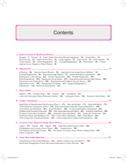
RMS values computed for each contraction level over 5 s.
Almost-linear trends of RMS values of
both EMG and VMG with muscular contraction:
useful in analysis of muscular activity.
EMG RMS vs force relationships vary
from muscle to muscle.
–813–
c R.M. Rangayyan, IEEE/Wiley
5. ANALYSIS OF WAVESHAPE
5.10. APPLICATION: CORRELATES OF MUSCULAR CONTRACTION
Figure 5.13: RMS values of the VMG and EMG signals for four levels of contraction of the rectus femoris muscle
at 60o knee-joint angle averaged over four subjects. Reproduced with permission from Y.T. Zhang, C.B. Frank,
R.M. Rangayyan, and G.D. Bell, Relationships of the vibromyogram to the surface electromyogram of the human
rectus femoris muscle during voluntary isometric contraction, Journal of Rehabilitation Research and Development,
c
33(4): 395–403, 1996. Department
of Veterans Affairs.
–814–
c R.M. Rangayyan, IEEE/Wiley
5. ANALYSIS OF WAVESHAPE
5.10. APPLICATION: CORRELATES OF MUSCULAR CONTRACTION
Figure 5.14: EMG RMS value versus level of muscle contraction expressed as a percentage of the maximal
voluntary contraction level (%MVC) for each subject. The relationship is displayed for three muscles. FDI: first
dorsal interosseus. N: number of muscles in the study. Reproduced with permission from J.H. Lawrence and C.J.
de Luca, Myoelectric signal versus force relationship in different human muscles, Journal of Applied Physiology,
c
54(6):1653–1659, 1983. American
Physiological Society.
–815–
c R.M. Rangayyan, IEEE/Wiley
5. ANALYSIS OF WAVESHAPE
5.10. APPLICATION: CORRELATES OF MUSCULAR CONTRACTION
–816–
c R.M. Rangayyan, IEEE/Wiley