1. science
2. mathematics
3. geometry

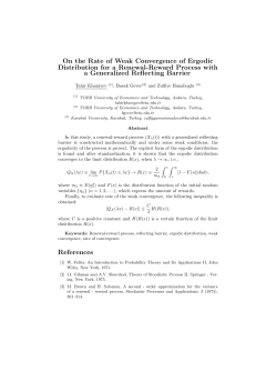
Annales de l’Institut Henri Poincaré - Probabilités et Statistiques
2015, Vol. 51, No. 2, 545–556
DOI: 10.1214/13-AIHP586
© Association des Publications de l’Institut Henri Poincaré, 2015
www.imstat.org/aihp
Weak convergence to stable Lévy processes for nonuniformly
hyperbolic dynamical systems
Ian Melbournea,1 and Roland Zweimüllerb
a Mathematics Institute, University of Warwick, Coventry, CV4 7AL, UK. E-mail: [email protected]
b Faculty of Mathematics, University of Vienna, Vienna, Austria. E-mail: [email protected]
Received 28 February 2013; revised 20 September 2013; accepted 22 September 2013
Abstract. We consider weak invariance principles (functional limit theorems) in the domain of a stable law. A general result is
obtained on lifting such limit laws from an induced dynamical system to the original system. An important class of examples
covered by our result are Pomeau–Manneville intermittency maps, where convergence for the induced system is in the standard
Skorohod J1 topology. For the full system, convergence in the J1 topology fails, but we prove convergence in the M1 topology.
Résumé. Nous considérons des principes d’invariance faibles (théorèmes limites fonctionnels) dans le domaine d’une loi stable.
Un résultat général est obtenu en relevant de telles lois limites depuis un système dynamique induit vers le système original. Une
classe importante d’exemples couverte par notre résultat est donnée par les transformations intermittentes à la Pomeau–Manneville,
où la convergence pour le système induit est dans la topologie J1 de Skorohod standard. Pour le système complet, il n’y a pas de
convergence dans la topologie J1 , mais nous prouvons la convergence dans la topologie M1 .
MSC: Primary 37D25; secondary 28D05; 37A50; 60F17
Keywords: Nonuniformly hyperbolic systems; Functional limit theorems; Lévy processes; Induced dynamical systems
1. Introduction
For large classes of dynamical systems with good mixing properties, it is possible to obtain strong statistical limit
laws such as the central limit theorems and its refinements including the almost sure invariance principle (ASIP) [5,
10,12,15,20,21,25–27]. An immediate consequence of the ASIP is the weak invariance principle (WIP) which is the
focus of this paper.
Thus the standard WIP (weak convergence to Brownian motion) holds for general Axiom A diffeomorphisms and
flows, and also for nonuniformly hyperbolic maps and flows modelled by Young towers [35,36] with square integrable
return time function (including Hénon-like attractors [7], finite horizon Lorentz gases [25], and the Lorenz attractor
[22]).
Recently, there has been interest in statistical limit laws for dynamical systems with weaker mixing properties such
as those modelled by a Young tower where the return time function is not square integrable. In the borderline case
where the return time lies in Lp for all p < 2, it is often possible to prove a central limit theorem with nonstandard
norming (nonstandard domain of attraction of the normal distribution). This includes important examples such as the
infinite horizon Lorentz gas [32], the Bunimovich stadium [4] and billiards with cusps [3]. In such cases, it is also
possible to obtain the corresponding WIP (see, for example, [3,11]).
1 The research of Ian Melbourne was supported in part by EPSRC Grant EP/F031807/1 held at the University of Surrey.
546
I. Melbourne and R. Zweimüller
For Young towers with return time function that is not square-integrable, the central limit theorem generally fails.
Gouëzel [18] (see also Zweimüller [37]) obtained definitive results on convergence in distribution to stable laws. The
only available results on the corresponding WIP are due to Tyran-Kami´nska [33] who gives necessary and sufficient
conditions for weak convergence to the appropriate stable Lévy process in the standard Skorohod J1 topology [31].
However in the situations we are interested in, the J1 topology is too strong and the results in [33] prove that weak
convergence fails in this topology.
In this paper, we repair the situation by working with the M1 topology (also introduced by Skorohod [31]). In
particular, we give general conditions for systems modelled by a Young tower, whereby convergence in distribution
to a stable law can be improved to weak convergence in the M1 topology to the corresponding Lévy process.
The proof is by inducing (see [19,28,30] for proofs by inducing of convergence in distribution). Young towers by
definition have a good inducing system, namely a Gibbs–Markov map (a Markov map with bounded distortion and
big images [1]). The results of Tyran-Kami´nska [33] often apply positively for such induced maps (see for example
the proof of Theorem 4.1 below) and yield weak convergence in the J1 topology, and hence the M1 topology, for the
induced system. The main theoretical result of the present paper discusses how M1 convergence in an induced system
lifts to the original system (even when convergence in the J1 topology does not lift).
As a special case, we recover the aforementioned results [3,11] on the WIP in the nonstandard domain of attraction
of the normal distribution.
In the remainder of the Introduction, we describe how our results apply to Pomeau–Manneville intermittency maps
[29]. In particular, we consider the family of maps f : X → X, X = [0, 1], studied by [23], given by
x(1 + 2γ x γ ), x ∈ [0, 12 ],
f (x) =
(1.1)
2x − 1,
x ∈ ( 12 , 1].
For γ ∈ [0, 1), there is a unique absolutely continuous ergodic invariant probability measure μ. Suppose that φ : X →
j
R is a Hölder observable with X φ dμ = 0. Let φn = n−1
j =0 φ ◦ f . For the map in (1.1), our main result implies the
following:
Theorem 1.1. Let f : [0, 1] → [0, 1] be the map (1.1) with γ ∈ ( 12 , 1) and set α = 1/γ . Let φ : [0, 1] → R be a mean
zero Hölder observable and suppose that φ(0) = 0. Define Wn (t) = n−1/α φnt . Then Wn converges weakly in the
Skorohod M1 topology to an α-stable Lévy process. (The specific Lévy process is described below.)
Remark 1.2. The J1 and M1 topologies are reviewed in Section 2.1. Roughly speaking, the difference is that the M1
topology allows numerous small jumps for Wn to accumulate into a large jump for W , whereas the J1 topology would
require a large jump for W to be approximated by a single large jump for Wn . Since the jumps in Wn are bounded by
n−1/α |φ|∞ , it is evident that in Theorem 1.1 convergence cannot hold in the J1 topology.
Situations in the probability theory literature where convergence holds in the M1 topology but not the J1 topology
include [2,6].
Theorem 1.1 completes the study of weak convergence for the intermittency map (1.1) with γ ∈ [0, 1) and typical
Hölder observables. We recall the previous results in this direction. If γ ∈ [0, 12 ) then it is well known that φ satisfies
a central limit theorem, so n−1/2 φn converges in distribution to a normal distribution with mean zero and variance
σ 2 , where σ 2 is typically positive. Moreover, [25] proved the ASIP. An immediate consequence is the WIP: Wn (t) =
n−1/2 φnt converges weakly to Brownian motion.
If γ = 12 and φ(0) = 0, then Gouëzel [18] proved that φ is in the nonstandard domain of attraction of the normal
distribution: (n log n)−1/2 φn converges in distribution to a normal distribution with mean zero and variance σ 2 > 0.
Dedecker and Merlevede [11] obtained the corresponding WIP in this situation (with Wn (t) = (n log n)−1/2 φnt ).
Finally, if γ ∈ ( 12 , 1) and φ(0) = 0, then Gouëzel [18] proved that n−1/α φn converges in distribution to a one-sided
stable law G with exponent α = γ −1 . The stable law in question has characteristic function
E eitG = exp −c|t|α 1 − i sgn φ(0)t tan(απ/2) ,
where c = 14 h( 12 )(α|φ(0)|)α Γ (1 − α) cos(απ/2) and h = dμ
dx is the invariant density. Let {W (t); t ≥ 0} denote the
corresponding α-stable Lévy process (so {W (t)} has independent and stationary increments with cadlag sample paths
Convergence to stable Levy processes for dynamical systems
547
and W (t) =d t 1/α G). Tyran-Kami´nska [33] verified that Wn (t) = n−1/α φnt does not converge weakly to W in the
J1 topology. In contrast, Theorem 1.1 shows that Wn converges weakly to W in the M1 topology.
The remainder of this paper is organised as follows. In Section 2 we state our main abstract result, Theorem 2.2,
on inducing the WIP. In Section 3 we prove Theorem 2.2. In Section 4 we consider some examples which include
Theorem 1.1 as a special case.
2. Inducing a weak invariance principle
In this section, we formulate our main abstract result Theorem 2.2. The result is stated in Section 2.2 after some
preliminaries in Section 2.1.
2.1. Preliminaries
Distributional convergence. To fix notations, let (X, P ) be a probability space and (Rn )n≥1 a sequence of Borel
measurable maps Rn : X → S, where (S, d) is a separable metric space. Then distributional convergence of (Rn )n≥1
P
L(μ)
w.r.t. P to some random element R of S will be denoted by Rn ⇒ R. Strong distributional convergence Rn ⇒ R
P
on a measure space (X, μ) means that Rn ⇒ R for all probability measures P μ.
Skorohod spaces. We briefly review the required background material on the Skorohod J1 and M1 topologies [31]
on the linear spaces D[0, T ], D[T1 , T2 ], and D[0, ∞) of real-valued cadlag functions (right-continuous g(t + ) = g(t)
with left-hand limits g(t − )) on the respective interval, referring to [34] for proofs and further information. Both
topologies are Polish, with J1 stronger than M1 .
It is customary to first deal with bounded time intervals. We thus fix some T > 0 and focus on D = D[0, T ].
(Everything carries over to D[T1 , T2 ] in an obvious fashion.) Throughout, · will denote the uniform norm. Two
functions g1 , g2 ∈ D are close in the J1 -topology if they are uniformly close after a small distortion of the domain.
Formally, let Λ be the set of increasing homeomorphisms λ : [0, T ] → [0, T ], and let λid ∈ Λ denote the identity. Then
dJ1 ,T (g1 , g2 ) = infλ∈Λ {g1 ◦ λ − g2 ∨ λ − λid } defines a metric on D which induces the J1 -topology. While its
restriction to C = C[0, T ] coincides with the uniform topology, discontinuous functions are J1 -close to each other if
they have jumps of similar size at similar positions.
In contrast, the M1 -topology allows a function g1 with a jump at t to be approximated arbitrarily well by some
continuous g2 (with large slope near t ). For convenience, we let [a, b] denote the (possibly degenerate) closed interval
with endpoints a, b ∈ R, irrespective of their order. Let Γ (g) := {(t, x) ∈ [0, T ] × R: x ∈ [g(t − ), g(t)]} denote the
completed graph of g, and let Λ∗ (g) be the set of all its parametrizations, that is, all continuous G = (λ, γ ) : [0, T ] →
Γ (g) such that t < t implies either λ(t ) < λ(t) or λ(t ) = λ(t) plus |γ (t) − g(λ(t))| ≤ |γ (t ) − g(λ(t))|. Then
dM1 ,T (g1 , g2 ) = infGi =(λi ,γi )∈Λ∗ (gi ) {λ1 − λ2 ∨ γ1 − γ2 } gives a metric inducing M1 .
∞
On the space D[0, ∞) the τ -topology, τ ∈ {J1 , M1 }, is defined by the metric dτ,∞ (g1 , g2 ) := 0 e−t (1 ∧
dτ,t (g1 , g2 )) dt. Convergence gn → g in (D[0, ∞), τ ) means that dτ,T (gn , g) → 0 for every continuity point T of g.
For either topology, the corresponding Borel σ -field BD,τ on D, generated by the τ -open sets, coincides with the
usual σ -field BD generated by the canonical projections πt (g) := g(t). Therefore, any family W = (Wt )t∈[0,T ] or
(Wt )t∈[0,∞) of real random variables Wt such that each path t → Wt is cadlag, can be regarded as a random element
of D, equipped with τ = J1 or M1 .
2.2. Statement of the main result
Recall that for any ergodic measure preserving transformation (m.p.t.) f on a probability space (X, μ), and any
Y ⊂ X withμ(Y ) > 0, the return time function r : Y → N ∪ {∞} given by r(y) := inf{k ≥ 1: f k (y) ∈ Y } is integrable
with mean Y r dμY = μ(Y )−1 (Kac’ formula), where μY (A) := μ(Y ∩ A)/μ(Y ). Moreover, the first return map or
induced map F := f r : Y → Y is an ergodic m.p.t. on the probability space (Y, μY ). This is widely used as a tool in
the study of complicated systems, where Y is chosen in such a way that F is more convenient than f . In particular,
given an observable (i.e., a measurable
function) φ : X → R, it may be easier to first consider its induced version
1
1
φ
Φ : Y → R on Y , given by Φ := r−1
=0 ◦ f . By standard arguments, if φ ∈ L (X, μ) then Φ ∈ L (Y, μY ) and
548
I. Melbourne and R. Zweimüller
Φ dμY = μ(Y )−1 X φ dμ. In this setup, we will denote the corresponding ergodic sums by φk := k−1
=0 φ ◦ f and
n−1
j
Φn := j =0 Φ ◦ F , respectively.
Our core result allows us to pass from a weak invariance principle for the induced version to one for the original
observable. Such a step requires some a priori control of the behaviour of ergodic sums φk during an excursion from Y .
We shall express this in terms of the function Φ ∗ : Y → [0, ∞] given by
Φ ∗ (y) :=
φ (y) − φ (y) ∧
φ (y) − φ (y) .
max
max
Y
0≤ ≤≤r(y)
0≤ ≤≤r(y)
Note that Φ ∗ vanishes if and only if the ergodic sums φk grow monotonically (nonincreasing or nondecreasing) during
each excursion. Hence bounding Φ ∗ means limiting the growth of φ until the first return to Y in at least one direction.
↑
↓
The expression Φ ∗ can be understood also in terms of the maximal and minimal processes φ , φ defined during each
excursion 0 ≤ ≤ r(y) by
↑
φ (y) = max φ (y),
0≤ ≤
↓
φ (y) = min
φ (y).
0≤ ≤
Proposition 2.1.
(i) In the “predominantly increasing” case Φ ∗ (y) = max0≤ ≤≤r(y) (φ (y) − φ (y)), we have Φ ∗ (y) =
↑
max0≤≤r(y) (φ (y) − φ (y)).
(ii) In the “predominantly decreasing” case Φ ∗ (y) = max0≤ ≤≤r(y) (φ (y) − φ (y)), we have Φ ∗ (y) =
↓
max0≤≤r(y) (φ (y) − φ (y)).
↑
↓
Proof. This is immediate from the definition of φ and φ .
We use Φ ∗ to impose a weak monotonicity condition for φ during excursions.
Theorem 2.2 (Inducing a weak invariance principle). Let f be an ergodic m.p.t. on the probability space (X, μ),
and let Y ⊂ X be a subset of positive measure with return time r and first return map F . Suppose that the observable
φ : X → R is such that its induced version Φ satisfies a WIP on (Y, μY ) in that
L(μY ) Φtn
(2.1)
⇒ W (t) t≥0 in D[0, ∞), M1 ,
Pn (t) t≥0 :=
B(n) t≥0
where B is regularly varying of index γ > 0, and (W (t))t≥0 is a process with cadlag paths. Moreover, assume that
μ
1 Y
0.
max Φ ∗ ◦ F j ⇒
B(n) 0≤j ≤n
Then φ satisfies a WIP on (X, μ) in that
L(μ) φsn
⇒ W sμ(Y ) s≥0
Wn (s) s≥0 :=
B(n) s≥0
(2.2)
in D[0, ∞), M1 .
(2.3)
Remark 2.3 (α-stable processes).
If the process W in (2.1) for the induced system is an α-stable Lévy process, then
the limiting process in (2.3) is ( Y r dμY )−1/α W .
Remark 2.4. In general, the convergence from (2.3) fails in (D[0, ∞), J1 ), even if (2.1) holds in the J1 -topology.
That this is the case for the intermittent maps (1.1) was pointed out in [33], Example 2.1.
Remark 2.5 (Continuous sample paths). If the process W in (2.1) for the induced system has continuous sample
paths, then the statement and proof of Theorem 2.2 is greatly simplified and the uniform topology (corresponding to the
Convergence to stable Levy processes for dynamical systems
549
uniform norm ·) can be used throughout. In particular, the function Φ ∗ is replaced by Φ ∗ (y) = max0≤<r(y) |φ (y)|.
In the case of normal diffusion B(n) = n1/2 , condition (2.2) is then satisfied if Φ ∗ ∈ L2 .
A simplified proof based on the one presented here is written out in [17], Appendix.
Remark 2.6 (Centering). In the applications that we principally have in mind (including the maps (1.1)), the observable φ : X → R is integrable, and hence so is its induced version Φ : Y → R. In particular, if φ has mean zero, then Φ
has mean zero and we are in a situation to apply Theorem 2.2. From this, it follows easily that if condition (2.1) holds
with
Φtn − tn Y Φ dμY
Pn (t) =
,
B(n)
and condition (2.2) holds with φ replaced throughout by φ − X φ dμ in the definition of Φ ∗ , then conclusion (2.3) is
valid with
φsn − sn X φ dμ
Wn (s) =
.
B(n)
With a little more effort it is also possible to handle more general centering sequences where the process (Pn ) in
condition (2.1) takes the form
Pn (t) =
Φtn − tA(n)
,
B(n)
for real sequences A(n), B(n) with B(n) → ∞.
The monotonicity condition (2.2) will be shown to hold, for example, if we have sufficiently good pointwise control
for single excursions:
Proposition 2.7 (Pointwise weak monotonicity). Let f be an ergodic m.p.t. on the probability space (X, μ), and let
Y ⊂ X be a subset of positive measure with return time r. Let B be regularly varying of index γ > 0. Suppose that for
the observable φ : X → R there is some η ∈ (0, ∞) such that for a.e. y ∈ Y ,
Φ ∗ (y) ≤ ηB r(y) .
(2.4)
Then the weak monotonicity condition (2.2) holds.
The proofs of Theorem 2.2 and Proposition 2.7 are given in Section 3.
L(μY )
μ
Y
is not a restriction, as an application of
Assuming strong distributional convergence ⇒ in (2.1), rather than ⇒,
the following result to the induced system (Y, μY , F ) shows.
Proposition 2.8 (Automatic strong distributional convergence). Let f be an ergodic m.p.t. on a σ -finite space
(X, μ). Let τ = J1 or M1 and let A(n), B(n) be real sequences with B(n) → ∞. Assume that φ : X → R is measurable, and that there is some probability measure P μ and some random element R of D[0, ∞) such that
φtn − tA(n)
P
⇒ R in D[0, ∞), τ .
(2.5)
Rn :=
B(n)
t≥0
L(μ)
Then, Rn ⇒ R in (D[0, ∞), τ ).
Proof. This is based on ideas in [14]. According to Zweimüller [38], Theorem 1, it suffices to check that dτ,∞ (Rn ◦
μ
f, Rn ) −→ 0. The proof of [38], Corollary 3, shows that B(n) → ∞ alone (that is, even without (2.5)) implies
μ
dJ1 ,∞ (Rn ◦ f, Rn ) −→ 0. Since dM1 ,∞ ≤ dJ1 ,∞ (see [34], Theorem 12.3.2), the case τ = M1 then is a trivial
consequence.
550
I. Melbourne and R. Zweimüller
Remark 2.9. There is a systematic typographical error in [38] in that the factor t in the centering process tA(n)/B(n)
is missing, but the arguments there work, without any change, for the correct centering.
3. Proof of Theorem 2.2
In this section, we give the proof of Theorem 2.2 and also Proposition 2.7. Throughout, we assume the setting of
Theorem 2.2. In particular, we suppose that f is an ergodic m.p.t. on the probability space (X, μ), and that Y ⊂ X is
a subset of positive measure with return time r and first return map F .
3.1. Decomposing the processes
When Y is chosen appropriately, many features of f are reflected in the behaviour of the ergodic sums rn = n−1
j =0 r ◦
F j , i.e., the times at which orbits return to Y . These are intimately related to the occupation times or lap numbers
Nk :=
k
1Y ◦ f = max{n ≥ 0: rn ≤ k} ≤ k,
k ≥ 0.
=1
The visits to Y counted by the Nk separate the consecutive excursions from Y , that is, the intervals {rj , . . . , rj +1 − 1},
j ≥ 0. Decomposing the f -orbit of y into these excursions, we can represent the ergodic sums of φ as
φk = ΦNk + Rk
on Y
Nk encoding the contribution of the incomplete last excursion
with remainder term Rk = k−1
=rNk φ ◦ f = φk−rNk ◦ F
(if any). Next, decompose the rescaled processes accordingly, writing
Wk (s) = Uk (s) + Vk (s),
with Uk (s) := B(k)−1 ΦNsk , and Vk (s) := B(k)−1 Rsk . On the time scale of Un , the excursions correspond to the
intervals [tn,j , tn,j +1 ), j ≥ 0, where tn,j : Y → [0, ∞) is given by tn,j := rj /n. Note that the interval containing a
given point t > 0 is that with j = Ntn . Hence
t ∈ [tn,Ntn , tn,Ntn +1 )
for t > 0 and n ≥ 1.
(3.1)
3.2. Some almost sure results
In this subsection, we record some consequences of the ergodic theorem which we will use below. But first an elementary observation, the proof of which we omit.
Lemma 3.1. Let (cn )n≥0 be a sequence in R such that n−1 cn → c ∈ R. Define a sequence of functions Cn : [0, ∞) →
R by letting Cn (t) := n−1 ctn − tc. Then, for any T > 0, (Cn )n≥1 converges to 0 uniformly on [0, T ].
For the occupation times of Y , we then obtain:
Lemma 3.2 (Strong law of large numbers for occupation times). The occupation times Nk satisfy
(a) k −1 Nk −→ μ(Y ) a.e. on X as k → ∞.
(b) Moreover, for any T > 0,
sup k −1 Ntk − tμ(Y ) −→ 0 a.e. on X as k → ∞.
t∈[0,T ]
Proof. The first statement is immediate from the ergodic theorem. The second then follows by the preceding
lemma.
Convergence to stable Levy processes for dynamical systems
551
Lemma 3.3. For any T > 0, limn→∞ n−1 max0≤j ≤T n+1 (r ◦ F j ) = 0 a.e. on Y .
Proof. Applying the ergodic theorem to F and the integrable function r, we get n−1
hence also n−1 (r ◦ F n ) → 0 a.e. on Y . The result follows from Lemma 3.1.
n−1
j =0 r
◦ F j → μ(Y )−1 , and
Pointwise control of monotonicity behaviour. We conclude this subsection by establishing Proposition 2.7.
Proof of Proposition 2.7. We may suppose without loss that the sequence B(n) is nondecreasing. Since this seδ > 0. Hence for δ > 0 fixed, there are δ > 0 and n ≥ 1 s.t.
quence is regularly varying, B(
δ n)/B(n) → δ γ for all ηB(h)/B(n) < δ whenever n ≥ n and h ≤ δ n.
As a consequence of Lemma 3.3, there is some n ≥ 1 such that Yn := {n−1 max0≤j ≤n (r ◦ F j ) < δ } satisfies
μY (Ync ) < δ for n ≥ n. In view of (2.4) we then see (using monotonicity of B again) that
1 1 max Φ ∗ ◦ F j ≤
max ηB r ◦ F j
B(n) 0≤j ≤n
B(n) 0≤j ≤n
≤
ηB(max0≤j ≤n (r ◦ F j ))
<δ
B(n)
n,
on Yn for n ≥ which proves (2.2).
3.3. Convergence of (Un )
As a first step towards Theorem 2.2, we prove that switching from Φtn to ΦNsk preserves convergence in the
Skorohod space.
Lemma 3.4 (Convergence of (Un )). Under the assumptions of Theorem 2.2,
μY Un (s) s≥0 ⇒ W sμ(Y ) s≥0 in D[0, ∞), M1 .
Proof. For n ≥ 1 and s ∈ [0, ∞), we let un (s) := n−1 Nsn . Since un (s)n = Nsn , we have
Un (s) = Pn un (s) on Y for n ≥ 1 and s ≥ 0.
(3.2)
We regard Un , Pn , W , and un as random elements of (D, M1 ) = (D[0, ∞), M1 ). Note that un ∈ D↑ := {g ∈
D: g(0) ≥ 0 and g nondecreasing}. Let u denote the constant random element of D given by u(s)(y) := sμ(Y ),
s ≥ 0.
Recalling Lemma 3.2(b), we see that for μY -a.e. y ∈ Y we have un (·)(y) → u(·)(y) uniformly on compact subsets
of [0, ∞). Hence, un → u in (D, M1 ) holds μY -a.e. In particular,
μ
Y
u
un ⇒
in (D, M1 ).
L(μY )
By assumption (2.1) we also have Pn ⇒ W in (D, M1 ). But then we automatically get
μY
(Pn , un ) ⇒ (W, u) in (D, M1 )2 ,
(3.3)
since the limit u of the second component is deterministic.
The composition map (D, M1 ) × (D↑ , M1 ) → (D, M1 ), (g, v) → g ◦ v, is continuous at every pair (g, v) with
v ∈ C↑↑ := {g ∈ D: g(0) ≥ 0 and g strictly increasing and continuous}, cf. [34], Theorem 13.2.3. As the limit (W, u)
in (3.3) satisfies Pr((W, u) ∈ D × C↑↑ ) = 1, the standard mapping theorem for distributional convergence (cf. [34],
Theorem 3.4.3) applies to (Pn , un ), showing that
μY
Pn ◦ un ⇒ W ◦ u in (D, M1 ).
In view of (3.2), this is what was to be proved.
552
I. Melbourne and R. Zweimüller
3.4. Control of excursions
Passing from convergence of (Un ) to convergence of (Wn ) requires a little preparation.
Lemma 3.5. (i) Let g, g ∈ D[0, T ] and 0 = T0 < · · · < Tm = T . Then
dM1 ,T g, g ≤ max dM1 ,[Tj −1 ,Tj ] g|[Tj −1 ,Tj ] , g |[Tj −1 ,Tj ] .
1≤j ≤m
(ii) Let gj ∈ D[Tj −1 , Tj ] and g¯ j := 1[Tj −1 ,Tj ) gj (Tj −1 ) + 1{Tj } gj (Tj ). Then
dM1 ,[Tj −1 ,Tj ] (gj , g¯ j ) ≤ 2gj∗ + (Tj − Tj −1 ),
where gj∗ := (supTj −1 ≤s≤t≤Tj (gj (s) − gj (t))) ∧ (supTj −1 ≤s≤t≤Tj (gj (t) − gj (s))).
Proof. The first assertion is obvious. To validate the second, assume without loss that j = 1 and that g1 is predom↑
inantly increasing in that g1∗ = supT0 ≤s≤t≤T1 (g1 (s) − g1 (t)). In this case, g1∗ = supT0 ≤t≤T1 (g1 (t) − g1 (t)) for the
↑
nondecreasing function g1 (t) := supT0 ≤s≤t g1 (s). Therefore,
↑
↑
dM1 ,[T0 ,T1 ] g1 , g1 ≤ g1 − g1 = g1∗ .
↑
↑
↑
Letting g¯ 1 := 1[T0 ,T1 ) g1 (T0 ) + 1{T1 } g1 (T1 ), it is clear that
↑
↑ ↑
dM1 ,[T0 ,T1 ] g¯ 1 , g¯ 1 ≤ g¯ 1 − g¯ 1 = g1 (T1 ) − g1 (T1 ) ≤ g1∗ .
Finally, we check that
↑ ↑
dM1 ,[T0 ,T1 ] g1 , g¯ 1 ≤ T1 − T0 .
↑
↑
↑
↑
To this end, we refer to Fig. 1 where Γ1 = Γ (g1 ) and Γ2 = Γ (g¯ 1 ) represent the completed graphs of g1 and g¯ 1
respectively. Here Γ2 consists of one horizontal line segment followed by one vertical segment. The picture of Γ1 is
schematic, it may also contain horizontal and vertical line segments.
Choose C on the graph of Γ1 that is equidistant from AD and DB and let E be the point on DB that is the same
height as C. Choose parametrizations Gi = (λi , γi ) of Γi , i = 1, 2, satisfying
(i) G1 (0) = G2 (0) = A, G1 (1) = G2 (1) = B,
(ii) G1 ( 12 ) = C, G2 ( 12 ) = E,
(iii) γ1 (t) = γ2 (t) for all t ∈ [ 12 , 1].
Automatically λ1 − λ2 ≤ |AD| = T1 − T0 and by construction γ1 − γ2 ≤ |DE| ≤ |AD|, as required.
Fig. 1. A monotone excursion.
Convergence to stable Levy processes for dynamical systems
553
As a consequence, we obtain:
Lemma 3.6. dM1 ,T (Wn , Un ) ≤ max0≤j ≤T n+1 (n−1 r + 2B(n)−1 Φ ∗ ) ◦ F j .
Proof. Let y ∈ Y and decompose [0, T ] according to the consecutive excursions, letting Tj := tn,j (y) ∧ T , j ≤ m :=
T n + 1. Consider g(t) := Wn (t)(y), t ∈ [0, T ]. If we set gj := g|[Tj −1 ,Tj ] , then g¯ j as defined in Lemma 3.5 coincides
with Un (·)(y)|[Tj −1 ,Tj ] , so that
dM1 ,T Wn (·)(y), Un (·)(y) ≤ max dM1 ,[Tj −1 ,Tj ] (gj , g¯ j ).
0≤j ≤m
But Tj − Tj −1 = n−1 r ◦ F j , and since gj (s) − gj (t) = B(n)−1 (φ − φ ) ◦ F j (y), for suitable 0 ≤ ≤ ≤ r, we see
that Lemma 3.5 gives
dM1 ,[Tj −1 ,Tj ] (gj , g¯ j ) ≤ n−1 r + 2B(n)−1 Φ ∗ ◦ F j ,
as required.
Proof of Theorem 2.2. Fix any T > 0. By Lemma 3.3, n−1 max0≤j ≤T n+1 (r ◦ F j ) → 0 a.e. and by assumption
μY
0. Hence Lemma 3.6 guarantees that
(2.2) B(n)−1 max0≤j ≤T n+1 (Φ ∗ ◦ F j ) ⇒
μ
Y
dM1 ,T (Wn , Un ) ⇒
0.
(3.4)
Recall also from Lemma 3.4 that
μY W sμ(Y ) 0≤s≤T
Un (s) 0≤s≤T ⇒
in D[0, T ], M1 .
(3.5)
It follows (see [8], Theorem 3.1) from (3.4) and (3.5) that
μY Wn (s) 0≤s≤T ⇒ W sμ(Y ) 0≤s≤T
in D[0, T ], M1 .
μ
Y
This immediately gives (Wn (s))t≥0 ⇒
(W (sμ(Y )))s≥0 in (D[0, ∞), M1 ). Strong distributional convergence as
asserted in (2.3) follows via Proposition 2.8.
4. Examples
We continue to suppose that f is an ergodic m.p.t. on a probability space (X, μ) with first return map F = f r : Y → Y
where μ(Y ) > 0. Suppose further that the induced map F : Y → Y is Gibbs–Markov with ergodic invariant probability
measure μY and partition β, and that r|a is constant for each a ∈ β. Let φ : X → R be an L∞ mean zero observable,
with induced observable Φ : Y → R.
Theorem 4.1. Suppose that φ is constant on f a for every a ∈ β and ∈ {0, . . . , r|a − 1}. If Φ lies in the domain
of an α-stable law, then Φ satisfies the WIP in (D, J1 ) with B(n) = n1/α . If in addition condition (2.2) holds, then φ
satisfies the WIP in (D, M1 ).
Proof. By [1], n−1/α Φn converges in distribution to the given stable law. The assumptions guarantee that the induced
observable Φ is constant on each Yj . Hence we can apply Tyran-Kami´nska [33], Corollary 4.1, to deduce that Φ
satisfies the corresponding α-stable WIP in (D, J1 ). In particular, condition (2.1) is satisfied. The final statement
follows from Theorem 2.2.
For certain examples, including Pomeau–Manneville intermittency maps, we can work with general Hölder observables, thus improving upon [33], Example 4.1. The idea is to decompose the observable φ into a piecewise constant
observable φ0 and a Hölder observable φ˜ in such a way that only φ0 “sees” the source of the anomalous behaviour.
554
I. Melbourne and R. Zweimüller
In the remainder of this section, we carry out this procedure for the maps (1.1) and thereby prove Theorem 1.1.
(Lemma 4.2 and Proposition 4.3 below hold in the general context of induced Gibbs–Markov maps.)
Fix θ ∈ (0, 1) and let dθ denote the symbolic metric on Y , so dθ (x, y) = θ s(x,y) where s(x, y) is the least
integer n ≥ 0 such that F n x, F n y lie in distinct elements of β. An observable Φ : Y → R is piecewise Lipschitz if Da (Φ) := supx,y∈a,x=y |Φ(x) − Φ(y)|/dθ (x, y) < ∞ for each a ∈ β, and Lipschitz if Φθ = |Φ|∞ +
supa∈β Da (Φ) < ∞. The space Lip of Lipschitz observables Φ : Y → R is a Banach space. Note that Φ is integrable
with a∈β μY (a)Da (Φ) < ∞ if and only if a∈β μY (a)1a Φθ < ∞.
Let L denote the transfer operator for F : Y → Y .
Lemma 4.2. (a) The essential spectral
radius of L : Lip → Lip is at most θ . (b) Suppose that Φ : Y → R is a piecewise
Lipschitz observable satisfying a∈β μY (a)1a Φθ < ∞. Then LΦ ∈ Lip.
Proof. This is standard. See, for example, [1], Theorem 1.6, for part (a) and [25], Lemma 2.2, for part (b).
Proposition 4.3. Let Φ : Y → R be a piecewise Lipschitz mean zero observable lying in Lp , for some p ∈ (1, 2).
Assume that a∈β μY (a)1a Φθ < ∞. Then maxj =0,...,n−1 n−γ Φj →d 0 for all γ > 1/p.
Proof. Suppose first that F is weak mixing (this assumption is removed below). Then L : Lip → Lip has no eigenvalues on the unit circle except for the simple eigenvalue at 1 (corresponding to constant functions). By Lemma 4.2(a),
there exists τ < 1 such that the remainder of
the spectrum of L lies strictly inside the ball of radius τ . In particular,
there is a constant C > 0 such that Ln v − v dμY ≤ Cτ n v for all v ∈ Lip, n ≥ 1.
j
ˆ
By Lemma 4.2(b), LΦ ∈ Lip. Hence χ = ∞
j =1 L Φ ∈ Lip. Following Gordin [16], write Φ = Φ + χ ◦ F − χ .
p
p
ˆ
Then Φ ∈ L (since χ ∈ Lip and Φ ∈ L ). Applying L to both sides and noting that L(χ ◦ F ) = χ , we obtain that
LΦˆ = 0. It follows that the sequence {Φˆ n ; n ≥ 1} defines a reverse martingale sequence.
By Burkholder’s inequality [9], Theorem 3.2,
n
n
1/2 p/2 1/p
2
j
2
j
ˆ
ˆ
ˆ
|Φn |p Φ ◦F
Φ ◦F
=
j =1
≤
n
p
j =1
1/p
ˆ p ◦ Fj
|Φ|
ˆ p n1/p .
= |Φ|
j =1
By Doob’s inequality [13] (see also [9], Equation (1.4), p. 20), | maxj =0,...,n−1 Φˆ j |p |Φˆ n |p n1/p . By Markov’s
p
inequality, for > 0 fixed, μY (| maxj =0,...,n−1 Φˆ j | ≥ nγ ) ≤ | maxj =0,...,n−1 Φˆ j |p /( p nγp ) n−(γp−1) → 0 as n →
∞. Hence maxj =0,...,n−1 n−γ Φˆ j →d 0. Since Φ and Φˆ differ by a bounded coboundary, maxj =0,...,n−1 n−γ Φj →d 0
as required.
It remains to remove the assumption about eigenvalues (other than 1) for L on the unit circle. Suppose that
there are
k such eigenvalues eiω , ω ∈ (0, 2π), = 1, . . . , k (including multiplicities). Then we can write Φ = Ψ0 + k=1 Ψ
where Ln Ψ0 θ ≤ Cτ n Ψ0 θ and LΨ = eiω Ψ . In particular, the above argument applies to Ψ0 , while LΨ = eiω Ψ ,
= 1, . . . , k.
A simple argument (see [24]) shows that Ψ ◦ F = e−iω Ψ for = 1, . . . , k, so that | nj=1 Ψ ◦ F j |∞ ≤ 2|eiω −
1|−1 |Ψ |∞ which is bounded in n. Hence the estimate for Φ follows from the one for Ψ0 .
Proof of Theorem 1.1. We verify the hypotheses of Theorem 2.2. A convenient inducing set for the maps (1.1) is Y =
[ 12 , 1]. Let φ0 = φ(0) − μ(Y )−1 φ(0)1Y . (The first term is the important one, and the second term is simply an arbitrary
choice that ensures that φ0 has mean zero while preserving the piecewise constant requirement in Theorem 4.1.) Write
φ = φ0 + φ˜ and note that φ˜ is a mean zero piecewise Hölder observable vanishing at 0. We have the corresponding
decomposition Φ = Φ0 + Φ˜ for the induced observables. By Theorem 4.1, Φ0 satisfies the WIP (in the J1 topology).
Let η denote the Hölder exponent
of φ. By the proof of [18], Theorem 1.3, φ˜ induces to a piecewise Lipschitz mean
˜ θ < ∞ for suitably chosen θ . Moreover [18] shows that Φ˜ lies in L2
zero observable Φ˜ satisfying a∈β μY (a)1a Φ
Convergence to stable Levy processes for dynamical systems
555
provided that η > γ − 12 . Exactly the same argument shows that Φ˜ lies in Lp provided η > γ − p1 . In particular, for
any η > 0, there exists p > 1/γ such that Φ˜ ∈ Lp . Since we are normalising by B(n) = n1/α = nγ , it follows from
Proposition 4.3 that Φ˜ does not contribute to the WIP.
˜ we deduce that Φ satisfies the WIP (in the J1 topology). In particular,
Combining the results for Φ0 and Φ,
condition (2.1) is satisfied.
It remains to verify condition (2.4). In fact, we show that Φ ∗ is bounded. Suppose that φ(0) > 0 (the case φ(0) < 0
is treated similarly). Choose > 0 such that φ > 0 on [0, ]. Define the decreasing sequence xn ∈ (0, 12 ) where
f (xn ) = xn−1 , x1 = 12 , and let k be such that xn ∈ (0, ) for all n ≥ k. Then for y ∈ Y , f y ∈ [0, ] for 0 ≤ ≤
r(y) − k.
Now observe that
(i) φ (y) − φ (y) ≤ 0 for 1 ≤ ≤ ≤ r(y) − k,
(ii) φ (y) − φ (y) ≤ k|φ|∞ for r(y) − k ≤ ≤ ≤ r(y),
(iii) φ (y) − φ (y) ≤ φr(y)−k (y) − φ (y) ≤ k|φ|∞ for 1 ≤ ≤ r(y) − k ≤ ≤ r(y).
Hence
Φ ∗ (y) ≤
max
0≤ ≤≤r(y)
≤ |φ|∞ +
as required.
φ (y) − φ (y)
max
1≤ ≤≤r(y)
φ (y) − φ (y) ≤ (k + 1)|φ|∞ ,
Remark 4.4. The arguments in the proof of Theorem 1.1 apply to a much wider class of examples, including intermittent maps with neutral periodic points or with multiple neutral fixed/periodic points. In such cases, condition (2.2) is
again automatically satisfied.
Acknowledgement
We are very grateful to the referee for very helpful suggestions that led to a significantly simplified proof of the main
result in this paper.
References
[1] J. Aaronson and M. Denker. Local limit theorems for partial sums of stationary sequences generated by Gibbs–Markov maps. Stoch. Dyn. 1
(2001) 193–237. MR1840194
[2] F. Avram and M. S. Taqqu. Weak convergence of sums of moving averages in the α-stable domain of attraction. Ann. Probab. 20 (1992)
483–503. MR1143432
[3] P. Bálint, N. Chernov and D. Dolgopyat. Limit theorems for dispersing billiards with cusps. Comm. Math. Phys. 308 (2011) 479–510.
MR2851150
[4] P. Bálint and S. Gouëzel. Limit theorems in the stadium billiard. Comm. Math. Phys. 263 (2006) 461–512. MR2207652
[5] P. Bálint and I. Melbourne. Decay of correlations and invariance principles for dispersing billiards with cusps, and related planar billiard
flows. J. Stat. Phys. 133 (2008) 435–447. MR2448631
ˇ
[6] G. Ben Arous and J. Cerný.
Scaling limit for trap models on Zd . Ann. Probab. 35 (2007) 2356–2384. MR2353391
[7] M. Benedicks and L.-S. Young. Markov extensions and decay of correlations for certain Hénon maps. Astérisque 261 (2000) 13–56.
MR1755436
[8] P. Billingsley. Convergence of Probability Measures, 2nd edition. Wiley Series in Probability and Statistics: Probability and Statistics. Wiley,
New York, 1999. MR1700749
[9] D. L. Burkholder. Distribution function inequalities for martingales. Ann. Probab. 1 (1973) 19–42. MR0365692
[10] J.-P. Conze and S. Le Borgne. Méthode de martingales et flow géodésique sur une surface de courbure constante négative. Ergodic Theory
Dynam. Systems 21 (2001) 421–441. MR1827112
[11] J. Dedecker and F. Merlevède. Weak invariance principle and exponential bounds for some special functions of intermittent maps. High
Dimensional Probability 5 (2009) 60–72. MR2797940
[12] M. Denker and W. Philipp. Approximation by Brownian motion for Gibbs measures and flows under a function. Ergodic Theory Dynam.
Systems 4 (1984) 541–552. MR0779712
556
I. Melbourne and R. Zweimüller
[13] J. L. Doob. Stochastic Processes. Wiley, New York, 1953. MR0058896
[14] G. K. Eagleson. Some simple conditions for limit theorems to be mixing. Teor. Verojatnost. i Primenen 21 (1976) 653–660. MR0428388
[15] M. J. Field, I. Melbourne and A. Török. Decay of correlations, central limit theorems and approximation by Brownian motion for compact
Lie group extensions. Ergodic Theory Dynam. Systems 23 (2003) 87–110. MR1971198
[16] M. I. Gordin. The central limit theorem for stationary processes. Soviet Math. Dokl. 10 (1969) 1174–1176. MR0251785
[17] G. A. Gottwald and I. Melbourne. Central limit theorems and suppression of anomalous diffusion for systems with symmetry. Preprint, 2012.
[18] S. Gouëzel. Central limit theorem and stable laws for intermittent maps. Probab. Theory Related Fields 128 (2004) 82–122. MR2027296
[19] S. Gouëzel. Statistical properties of a skew product with a curve of neutral points. Ergodic Theory Dynam. Systems 27 (2007) 123–151.
MR2297091
[20] S. Gouëzel. Almost sure invariance principle for dynamical systems by spectral methods. Ann. Probab. 38 (2010) 1639–1671. MR2663640
[21] F. Hofbauer and G. Keller. Ergodic properties of invariant measures for piecewise monotonic transformations. Math. Z. 180 (1982) 119–140.
MR0656227
[22] M. Holland and I. Melbourne. Central limit theorems and invariance principles for Lorenz attractors. J. London Math. Soc. 76 (2007) 345–364.
MR2363420
[23] C. Liverani, B. Saussol and S. Vaienti. A probabilistic approach to intermittency. Ergodic Theory Dynam. Systems 19 (1999) 671–685.
MR1695915
[24] I. Melbourne and M. Nicol. Statistical properties of endomorphisms and compact group extensions. J. London Math. Soc. 70 (2004) 427–446.
MR2078903
[25] I. Melbourne and M. Nicol. Almost sure invariance principle for nonuniformly hyperbolic systems. Comm. Math. Phys. 260 (2005) 131–146.
MR2175992
[26] I. Melbourne and M. Nicol. A vector-valued almost sure invariance principle for hyperbolic dynamical systems. Ann. Probab. 37 (2009)
478–505. MR2510014
[27] I. Melbourne and A. Török. Central limit theorems and invariance principles for time-one maps of hyperbolic flows. Comm. Math. Phys. 229
(2002) 57–71. MR1917674
[28] I. Melbourne and A. Török. Statistical limit theorems for suspension flows. Israel J. Math. 144 (2004) 191–209. MR2121540
[29] Y. Pomeau and P. Manneville. Intermittent transition to turbulence in dissipative dynamical systems. Comm. Math. Phys. 74 (1980) 189–197.
MR0576270
[30] M. Ratner. The central limit theorem for geodesic flows on n-dimensional manifolds of negative curvature. Israel J. Math. 16 (1973) 181–197.
MR0333121
[31] A. V. Skorohod. Limit theorems for stochastic processes. Teor. Veroyatnost. i Primenen. 1 (1956) 289–319. MR0084897
[32] D. Szász and T. Varjú. Limit laws and recurrence for the planar Lorentz process with infinite horizon. J. Stat. Phys. 129 (2007) 59–80.
MR2349520
[33] M. Tyran-Kami´nska. Weak convergence to Lévy stable processes in dynamical systems. Stoch. Dyn. 10 (2010) 263–289. MR2652889
[34] W. Whitt. Stochastic-Process Limits. Springer Series in Operations Research. Springer, New York, 2002. MR1876437
[35] L.-S. Young. Statistical properties of dynamical systems with some hyperbolicity. Ann. of Math. 147 (1998) 585–650. MR1637655
[36] L.-S. Young. Recurrence times and rates of mixing. Israel J. Math. 110 (1999) 153–188. MR1750438
[37] R. Zweimüller. Stable limits for probability preserving maps with indifferent fixed points. Stoch. Dyn. 3 (2003) 83–99. MR1971188
[38] R. Zweimüller. Mixing limit theorems for ergodic transformations. J. Theoret. Probab. 20 (2007) 1059–1071. MR2359068