
High Dynamic Range Imaging - +* Tudalenau Bangor Pages
This is a preprint of the article to be published in Wiley Encyclopedia of Electrical
and Electronics Engineering.
High Dynamic Range Imaging
Rafał K. Mantiuk, Karol Myszkowski and Hans-Peter Seidel
April 3, 2015
Abstract
High dynamic range (HDR) images and video contain pixels, which can represent much greater range of colors and brightness levels than that offered by existing, standard dynamic range images. Such “better pixels” greatly improve the
overall quality of visual content, making it appear much more realistic and appealing to the audience. HDR is one of the key technologies of the future imaging
pipeline, which will change the way the digital visual content is represented and
manipulated.
This article offers a broad review of the HDR methods and technologies with
the introduction on fundamental concepts behind the perception of HDR imagery.
It serves both as an introduction to the subject and review of the current stateof-the-art in HDR imaging. It covers the topics related capture of HDR content
with cameras and its generation with computer graphics methods; encoding and
compression of HDR images and video; tone-mapping for displaying HDR content
on standard dynamic range displays; inverse tone-mapping for up-scaling legacy
content for presentation on HDR displays; the display technologies offering HDR
range; and finally image and video quality metrics suitable for HDR content.
Contents
.
.
.
.
.
.
.
.
.
.
.
.
.
.
.
.
.
.
.
.
.
.
.
.
.
.
.
.
.
.
.
.
.
.
.
.
.
.
.
.
.
.
.
.
3
3
5
5
8
2 Fundamental concepts
2.1 Dynamic range . . . . . . . . . . . . . . . . . . .
2.2 The difference between LDR and HDR pixel values
2.3 Display models and gamma correction . . . . . . .
2.4 The logarithmic domain and the sensitivity to light
.
.
.
.
.
.
.
.
.
.
.
.
.
.
.
.
.
.
.
.
.
.
.
.
.
.
.
.
.
.
.
.
.
.
.
.
.
.
.
.
8
9
10
11
13
3 Image and video acquisition
3.1 Computer graphics . . . . . . . . . . . . . . . . . . . . . . . . . . .
3.2 RAW vs. JPEG images . . . . . . . . . . . . . . . . . . . . . . . . .
17
17
18
1 Introduction
1.1 Low vs. high dynamic range imaging . . . . . .
1.2 Device- and scene-referred image representations
1.3 HDRI: mature imaging technology . . . . . . . .
1.4 HDR imaging pipeline . . . . . . . . . . . . . .
Page 1 of 81
R. K. Mantiuk, K. Myszkowski and H.-P. Seidel High Dynamic Range Imaging
3.3
.
.
.
.
.
.
.
.
.
.
.
.
.
.
.
.
.
.
.
.
.
.
.
.
.
.
.
.
.
.
.
.
.
.
.
.
.
.
.
.
.
.
.
.
.
.
.
.
.
19
19
21
21
21
22
22
.
.
.
.
.
.
.
.
.
.
.
.
.
.
.
.
.
.
.
.
.
.
.
.
.
.
.
.
22
23
28
29
30
5 Tone mapping
5.1 Intents of tone mapping . . . . . . . . . . . . . . . . . . . . .
5.2 Algebra of tone mapping . . . . . . . . . . . . . . . . . . . .
5.3 Major approaches to tone mapping . . . . . . . . . . . . . . .
5.3.1 Illumination and reflectance separation . . . . . . . .
5.3.2 Forward visual model . . . . . . . . . . . . . . . . .
5.3.3 Forward and inverse visual models . . . . . . . . . . .
5.3.4 Constrained mapping problem . . . . . . . . . . . . .
5.4 Perceptual effects for the enhancement of tone-mapped images
.
.
.
.
.
.
.
.
.
.
.
.
.
.
.
.
.
.
.
.
.
.
.
.
.
.
.
.
.
.
.
.
31
31
33
36
37
40
41
42
44
6 Inverse tone mapping
6.1 Recovering dynamic range . . . . . . . . . . . . . . . . . . . . .
6.1.1 LDR pixel linearization . . . . . . . . . . . . . . . . . . .
6.1.2 Dynamic range expansion . . . . . . . . . . . . . . . . .
6.2 Suppression of contouring and quantization errors . . . . . . . . .
6.3 Recovering under- and over-saturated textures . . . . . . . . . . .
6.4 Exploiting image capturing artifacts for upgrading dynamic range
.
.
.
.
.
.
.
.
.
.
.
.
46
47
48
49
51
52
53
7 HDR display technology
7.1 Dual modulation . . . . . . . . . . . .
7.2 HDR displays . . . . . . . . . . . . . .
7.3 HDR projectors . . . . . . . . . . . . .
7.4 Light field displays in HDR applications
3.4
Time sequential multi-exposure techniques . . . . . . . .
3.3.1 Deghosting: handling camera and object motion
3.3.2 Video solutions . . . . . . . . . . . . . . . . . .
HDR sensors and cameras . . . . . . . . . . . . . . . .
3.4.1 Spatial exposure change . . . . . . . . . . . . .
3.4.2 Multiple sensors with beam splitters . . . . . . .
3.4.3 Solid state sensors . . . . . . . . . . . . . . . .
4 Storage and compression
4.1 HDR pixel formats and color spaces
4.2 HDR image file formats . . . . . . .
4.3 High bit-depth encoding for HDR .
4.4 Backward-compatible compression .
.
.
.
.
.
.
.
.
.
.
.
.
.
.
.
.
.
.
.
.
.
.
.
.
.
.
.
.
.
.
.
.
.
.
.
.
.
.
.
.
.
.
.
.
.
.
.
.
.
.
.
.
.
.
.
.
.
.
.
.
.
.
.
.
.
.
.
.
.
.
.
.
.
.
.
.
.
.
.
.
.
.
.
.
54
56
57
59
60
8 HDR image quality
8.1 Display-referred vs. luminance independent metrics .
8.2 Perceptually-uniform encoding for quality assessment
8.3 Visual difference predictor for HDR images . . . . .
8.4 Tone-mapping metrics . . . . . . . . . . . . . . . .
.
.
.
.
.
.
.
.
.
.
.
.
.
.
.
.
.
.
.
.
.
.
.
.
.
.
.
.
.
.
.
.
.
.
.
.
61
61
62
63
64
Page 2 of 81
.
.
.
.
.
.
.
.
.
.
.
.
.
.
.
.
.
.
.
.
.
.
.
.
R. K. Mantiuk, K. Myszkowski and H.-P. Seidel High Dynamic Range Imaging
1 Introduction
High dynamic range imaging (HDRI) offers a radically new approach of representing
colors in digital images and video. Instead of using the range of colors produced by
a given display device, HDRI methods manipulate and store all colors and brightness
levels visible to the human eye. Since the visible range of colors is much larger than the
range achievable by cameras or displays (see Fig. 1), HDR color space is in principle a
superset of all color spaces used in traditional standard dynamic range imaging.
The goal of this article is a systematic survey of all elements of HDRI pipeline
from image/video acquisition, then storage and compression, to display and quality
evaluation. Before a detailed presentation of underlying technology and algorithmic
solutions, at first we discuss basic differences between HDR and standard imaging,
which is still predominantly in use (Sec. 1.1). This brings us naturally to the problem
of image representation, which in HDRI directly attempts to grasp possibly complete
information on depicted scenes, while in standard imaging it is explicitly tailored to
display capabilities at all processing stages (Sec. 1.2). Finally, we survey possible
application areas of HDRI technology in Sec. 1.3, and we overview the content of this
article in Sec. 1.4.
1.1
Low vs. high dynamic range imaging
Although tremendous progress can be observed in recent years towards improving the
quality of captured and displayed digital images and video, the reproduction of real
world appearance, which is seamless and convincingly immersive, is still a farfetched
goal. The discretization in spatial and temporal domains can be considered as a conceptually important difference with respect to the inherently continuous real world,
however, the pixel resolution in ultra high definition (UHD) imaging pipelines and
achievable there framerates are not the key limiting factors. The problem is the restricted color gamut and even more constrained luminance and contrast ranges that are
captured by cameras and stored by the majority of image and video formats.
For instance, each pixel value in the JPEG image encoding is represented using
three 8-bit integer numbers (0-255) using the YCrCb color space. This color space
is able to store only a small part of visible color gamut, as illustrated in Fig. 1-left,
and an even smaller part of the luminance range that can be perceived by our eyes, as
illustrated in Fig. 1-right. Similar limitations apply to predominantly used profiles of
video standards MPEG/H.264.
While the so-called multiple RAW formats with 12–16 bit precision, which is determined by the sensor capabilities, are available on many modern cameras, a common practice is an immediate conversion to JPEG/MPEG at early stages of on-camera
processing. This leads to irrecoverable losses of information with respect to the capabilities of human vision, and clearly will be a limiting factor for upcoming image
processing, storage, and display technologies. To emphasize these limitations of traditional imaging technology it is often called low-dynamic range or simply LDR.
High dynamic range imaging overcomes those limitations by imposing pixel colorimetric precision, which enables representing all colors found in real world that can
be perceived by the human eye. This in turn enables depiction of a range of perceptual
Page 3 of 81
R. K. Mantiuk, K. Myszkowski and H.-P. Seidel High Dynamic Range Imaging
2
LCD Display [2006] (0.5-500 cd/m )
2
CRT Display (1-100 cd/m )
Moonless Sky
-5
3•10 cd/m
10
-6
-4
10
Full Moon
2
3
6•10 cd/m
0.01
1
100
4
10
Sun
2
9
2•10 cd/m
10
6
10
8
2
10
10
2
Luminance [cd/m ]
Figure 1: Left: the transparent solid represents the entire color gamut visible to the
human eye. The solid tapers towards the bottom as color perception degrades at lower
luminance levels. For comparison, the red solid inside represents a standard sRGB
(Rec. 709) color gamut, which is produced by a good quality display. Right: real-world
luminance values compared with the range of luminance that can be displayed on CRT
and LDR monitors. Most digital content is stored in a format that at most preserves
c
the dynamic range of typical displays. (Reproduced with permission from [108] Morgan & Claypool Publishers.)
cues that are not achievable with traditional imaging. HDRI can represent images of
luminance range fully covering the scotopic, mesopic and photopic vision, which leads
to different perception of colors, including the loss of color vision in dim conditions.
For example, due to the so-called Hunt’s effect we tend to regard objects more colorful
when they are brightly illuminated. To render enhanced colorfulness properly, digital
images must preserve information about the actual level of luminance of the original
scene, which is not possible in the case of traditional imaging.
Real-world scenes are not only brighter and more colorful than their digital reproductions, but also contain much higher contrast, both local between neighboring
objects, and global between distant objects. The visual system has evolved to cope
with such high contrast and its presence in a scene evokes important perceptual cues.
Traditional imaging, unlike HDRI, is not able to represent such high-contrast scenes.
Similarly, traditional images can hardly represent common visual phenomena, such
as self-luminous surfaces (sun, shining lamps) and bright specular highlights. They
also do not contain enough information to reproduce visual glare (brightening of the
areas surrounding shining objects) and a short-time dazzle due to sudden increase of
the brightness of a scene (e.g., when exposed to the sunlight after staying indoors). To
faithfully represent, store and then reproduce all these effects, the original scene must
be stored and treated using high fidelity HDR techniques.
Page 4 of 81
R. K. Mantiuk, K. Myszkowski and H.-P. Seidel High Dynamic Range Imaging
1.2
Device- and scene-referred image representations
To accommodate all discussed requirements imposed on HDRI, a common format of
data is required to enable their efficient transfer and processing on the way from HDR
acquisition to HDR display devices. This stays in contrast with a plethora of sensor and
camera vendor dependent RAW formats. Here again fundamental differences between
image formats used in traditional imaging and HDRI arise, which we address in this
section.
Commonly used LDR image formats (JPEG, PNG, TIFF, and so on) have been designed to accommodate the capabilities of display devices with little concern on visual
information that cannot be displayed on those devices. Therefore those formats can be
considered as device-referred (also known as output-referred), since they are tightly
coupled with the capabilities of a particular imaging device. Obviously, such devicereferred image representations only vaguely relate to the actual photometric properties
of depicted scenes. This makes difficult the high fidelity reproduction of scene appearance across display devices with drastically different contrast ranges, absolute lowest
and peak luminance values, and color gamuts.
Scene-referred representation of images, which encodes the actual photometric
characteristics of depicted scenes, provides an easy solution to this problem. Conversion from such a common representation, which directly corresponds to physical
luminance or spectral radiance values, to a format suitable for a particular device is the
responsibility of that device. This should guarantee the best possible rendering of the
HDR content, since only the device has all the information related to its limitations and
sometimes also viewing conditions (e.g. ambient illumination), which is necessary to
render the content properly. HDR file formats are examples of scene-referred encoding, as they usually represent either luminance or spectral radiance, rather than gamma
corrected and ready to display “pixel values”.
The problem of accuracy of scene-referred image representation arises in terms of
tolerable quantization error. For display-referred image formats the pixel precision is
directly imposed by the reproduction capabilities of target display devices. For scenereferred image representations the accuracy should not be tailored to any particular
imaging technology and, if efficiency of storing data is required, the capabilities of the
human visual system should act as the only limiting factor.
To summarize, the difference between HDRI and traditional LDR imaging is that
HDRI always operates on device-independent and high-precision data, so that the quality of the content is reduced only at the display stage, and only if a device cannot faithfully reproduce the content. This is contrary to traditional LDR imaging, where the
content is usually profiled for particular device and thus stripped from useful information at the acquisition stage or latest at the storage stage. Fig. 2 summarizes these basic
conceptual differences between LDR and HDR imaging.
1.3
HDRI: mature imaging technology
After over two decades of intensive research and development HDRI has recently
gained momentum and is affecting almost all fields of digital imaging. One of the first
to adopt HDRI were video game developers together with graphics card vendors. To-
Page 5 of 81
R. K. Mantiuk, K. Myszkowski and H.-P. Seidel High Dynamic Range Imaging
Figure 2: The advantages of HDR compared to LDR from the application point of view.
The quality of the LDR image have been reduced on purpose to illustrate potential
differences between the HDR and LDR visual contents as seen on an HDR display. The
given numbers serve as an example and are not meant to be a precise reference. For the
dynamic range definitions, sych as dB, refer to Table 1. Figure adapted from [108].
day virtually all video game engines perform rendering using HDR precision to deliver
more believable and appealing virtual reality imagery. Computer generated imagery
used in special effect production relies on HDR techniques to achieve the best match
between synthetic and real-world scenes, which are often captured with professional
video HDR cameras. Advertising in the automotive industry, which is committed to
avoid premature release of the car look that still should be presented in an attractive,
possibly difficult to access scenography, relies on rendered computer graphics cars.
The rendered cars are composited into HDR photographs and videos, while captured
at the same spot HDR spherical environment maps enable the realistic simulation of
car illumination due to the precise radiometric information. Lower-end HDR cameras
are often mounted in cars to improve the safety of driving and parking maneuvers in
all lighting conditions. HDR video is also required in all applications in which capturing temporal aspects of changes in the scene is required with high accuracy such as
monitoring of some industrial processes including welding, or surveillance systems, to
name just a few possible applications.
Consumer-level cameras commonly offer an HDR mode of shooting images, which
reduces the problem of under- and over-exposure, where deeply saturated image regions in the LDR photography are now filled with lively textures and other scene details. For more demanding camera users, who do not want to rely on the black box oncamera HDR processing, a number of software tools are available that enable blending
of multiple differently exposed images of the same scene into an HDR image with the
Page 6 of 81
R. K. Mantiuk, K. Myszkowski and H.-P. Seidel High Dynamic Range Imaging
full control of this process. The same software tools typically offer a full suite of HDR
image editing tools and well as tone mapping solutions to reduce the dynamic range in
an HDR image and make it displayable on existing displays. All those developments
make the HDR photography really popular as confirmed by over 3 millions uploaded
photographs that are tagged as HDR on Flickr.
On the display side, all key vendors experiment with local dimming technology
with a grid of LEDs as the backlight device, which significantly enhances the dynamic
range offered by those displays. The full-fledged HDR displays with even higher density of high luminous power LEDs, which in some cases requires active liquid-based
cooling systems, are available for high-end consumers as well as for professional users.
In the latter case dedicated HDR displays can emulate all existing LDR displays due to
their superior contrast range and color gamut, which greatly simplifies video material
postproduction and color grading, so that the appearance of the final distribution-ready
video version looks optimally on all display technologies. Dual-modulation technology
is also used in the context of large HDR projection systems in digital cinema applications, and inexpensive pico-projectors enable their local overlap on the screen, which
after careful calibration leads to contrast enhancement as well.
Besides its significant impact on existing imaging technologies that we can observe
today, HDRI radically changes the methods by which imaging data is processed, displayed and stored in several fields of science. Computer vision algorithms and imagebased rendering techniques greatly benefit from the increased precision of HDR images, which do not have over- or under-exposed regions often causing the algorithm
failure. Medical imaging has developed image formats (e.g. the DICOM format) that
partly cope with the shortcomings of traditional images, however they are supported
only by specialized hardware and software. HDRI gives the sufficient precision for
medical imaging and therefore its capture, processing and rendering techniques is used
also in this field. HDR techniques also find applications in astronomical imaging, remote sensing, industrial design, scientific visualization, forensics at crime spots, artifact digitization and appearance capture in cultural heritage and internet shopping.
The maturity of HDRI technologies is confirmed by ongoing standardization efforts
for HDR JPEG and MPEG. The research literature is also immense and summarized in
a number of textbooks [10, 57, 101, 108, 128]. Multiple guides for photographers and
CG artists have been released as well [18]. An interesting account of historical developments on dynamic range expansion in the art, traditional photography, and electronic
imaging has been presented in [97, 101].
All these exciting developments in HDRI may suggest that the transition of LDR
imaging pipelines into their full-fledged HDR versions is a revolutionary step that can
be compared to the quantum leap from black&white to color imaging [18]. Obviously,
during the transition time some elements of imaging pipeline may still rely on traditional LDR technology. This will require backward compatibility of HDR formats to
enable their use on LDR output devices such as printers, displays, and projectors. For
some of such devices the format extensions to HDR should be transparent, and standard
display-referred content should be directly accessible. However, more advanced LDR
devices may take advantage of HDR information by adjusting scene-referred content to
their technical capabilities through customized tone reproduction. Finally, the legacy
images and video should be upgraded when displayed on HDR devices, so that the
Page 7 of 81
R. K. Mantiuk, K. Myszkowski and H.-P. Seidel High Dynamic Range Imaging
best possible image quality is achieved (the so-called inverse tone mapping). In this
work we address all these important issues and we structure our text following the key
elements of HDRI pipeline, which we briefly introduce in the following section.
1.4
HDR imaging pipeline
This article presents a complete pipeline for HDR image and video processing from
acquisition, through compression and quality evaluation, to display (refer to Fig. 3). At
the first stage digital images are acquired either with cameras or computer rendering
methods (Sec. 3). At the second stage, digital content is efficiently compressed and
encoded either for storage or transmission purposes (Sec. 4). Finally, digital video or
images are displayed on display devices. Tone mapping is required to accommodate
HDR content to LDR devices (Sec. 5), and conversely LDR content upgrading (the
so-called inverse tone mapping) is necessary for displaying on HDR devices (Sec. 6).
Apart from considering technical capabilities of display devices (Sec. 7), the viewing
conditions such as ambient lighting and amount of light reflected by the display play an
important role for proper determination of tone mapping parameters. Quality metrics
are employed to verify algorithms at all stages of the pipeline (Sec. 8).
Figure 3: Imaging pipeline and available HDR technologies. (Reproduced with perc Morgan & Claypool Publishers.)
mission from [108] Additionally, a short background on contrast sensitivity and brightness perception
is given as well as the terminology used for dynamic range measures in digital photography, camera sensors, and displays is discussed (Sec. 2).
2 Fundamental concepts
This section introduces some fundamental concepts and definitions commonly used in
high dynamic range imaging. When discussing the algorithms and methods in the following sections, we will refer to these concepts. First, several definitions of a dynamic
range are reviewed. Then, the differences between LDR and HDR pixels are explained.
Page 8 of 81
R. K. Mantiuk, K. Myszkowski and H.-P. Seidel High Dynamic Range Imaging
name
formula
example
context
CR = (Ypeak /Ynoise ) : 1
500:1
displays
log exposure range
D = log10 (Ypeak ) − log10 (Ynoise )
L = log2 (Ypeak ) − log2 (Ynoise )
2.7 orders
9 stops
HDR imaging,
photography
peak signal to noise ratio
PSNR = 20 · log10 (Ypeak /Ynoise )
53 [dB]
digital cameras
contrast ratio
Table 1: Measures of dynamic range and their context of application. The example
column illustrates the same dynamic range expressed in different units (adapted from
[108]).
This is followed by the description of a display model, which explains the relation between LDR pixel values and the light emitted by a display. Finally, the last section
describes the relation between luminance in the logarithmic domain and the sensitivity
of the human visual system.
2.1
Dynamic range
In principle, the term dynamic range is used in engineering to define the ratio between
the largest and the smallest quantity under consideration. With respect to images, the
observed quantity is the luminance level and there are several measures of dynamic
range in use depending on the application. They are summarized in Table 1.
The contrast ratio is a measure used in display systems and defines the ratio between the luminance of the brightest color it can produce (white) and the darkest
(black). In case a display does not emit any light at zero level, as for instance in
HDR displays [135], the first controllable level above zero is considered as the darkest
to avoid infinity. The ratio is usually normalized so that the second value is always one,
for example 1000:1, rather than 100:0.1.
The log exposure range is a measure commonly adopted in high dynamic range
imaging to measure the dynamic range of scenes. Here the considered range is between
the brightest and the darkest luminance in a given scene. The range is calculated as
the difference between the logarithm (base 10) of the brightest and the darkest spots.
The advantage of using logarithmic values is that they better describe the perceived
difference in dynamic range than the contrast ratio. The values are usually rounded to
the first decimal fraction.
The exposure latitude is defined as the luminance range the film can capture minus
the luminance range of the photographed scene and is expressed using logarithm base
2 with precision up to 1/3 . The choice of logarithmic base is motivated by the scale
of exposure settings, aperture closure (f-stops) and shutter speed (seconds), where one
step doubles or halves the amount of captured light. Thus the exposure latitude tells the
photographers how large a mistake they can make in setting the exposure parameters
while still obtaining a satisfactory image. This measure is mentioned here, because its
units, stop steps or stops in short, are often used in HDR photography to define the
luminance range of a photographed scene alone.
Page 9 of 81
R. K. Mantiuk, K. Myszkowski and H.-P. Seidel High Dynamic Range Imaging
The signal to noise ratio (SNR) is most often used to express the dynamic range of
a digital camera. In this context, it is usually measured as the ratio of the intensity that
starts to saturate the image sensor to the minimum intensity that can be observed above
the noise level of the sensor. It is expressed in decibels [dB] using 20 times base-10
logarithm.
The physical range of luminance, captured by the above measures, does not necessarily correspond the perceived magnitude of the dynamic range. This is because our
contrast sensitivity is significantly reduced for lower luminance levels, such as those
we find at night or in a dim cinema. For that reasons, it has been proposed to use the
number of just-noticeable contrast differences (JNDs) that a given display is capable
of producing as a more relevant measure of the dynamic range [167]. The concept of
JNDs will be discussed in more details in Section 2.4.
The actual procedure to measure dynamic range is not well defined and therefore
the reported numbers may vary. For instance, display manufacturers often measure the
white level and the black level with a separate set of display parameters that are finetuned to achieve the highest possible number which is obviously overestimated and
no displayed image can show such a contrast. On the other hand, HDR images often
have very few light or dark pixels. An image can be low-pass filtered before the actual
dynamic range measure is taken to assure reliable estimation. Such filtering averages
the minimum luminance thus gives a reliable noise floor, and smoothes single pixels
with very high luminance thus gives a reasonable maximum amplitude estimate. Such
a measurement is more stable compared to the non-blurred maximum and minimum
luminance.
Perceivable dynamic range One important and often disputed aspect is the dynamic
range that can be perceived by the human eye. The light scattering on the optic of the
eye can effectively reduce the maximum luminance contrast that can be projected onto
to retina to 2–3 log-10 units [98, 100]. However, since the eye is in fact a highly active
sensor, which can rapidly change the gaze and locally adapt, people are believed to be
able to perceive simultaneously the scenes of 4 or even more log-10 units of dynamic
range [128, Sec. 6.2]. The effective perceivable dynamic range will vary significantly
from scene to scene, it is, therefore, impossible to provide a single number. However,
it has been shown in multiple studies that people prefer images of the dynamic range
higher than 100:1 or 1000:1 when presented on a HDR display [28,76,180]. Therefore,
it can be stated with high confidence that we can perceive and appreciate the scenes of
higher contrast than 1000:1. It must be noted, however, that the actual appreciable dynamic range will depend on the peak brightness of a scene (or a display). For example,
OLED displays offer very high dynamic range, but since their peak brightness is limited, most of that range lies in low-luminance range, in which our ability to distinguish
colors is severely limited.
2.2
The difference between LDR and HDR pixel values
It is important to make distinction between the pixel values that can be found in typical
LDR images and those that are stored in HDR images. Pixel values in HDR images
Page 10 of 81
R. K. Mantiuk, K. Myszkowski and H.-P. Seidel High Dynamic Range Imaging
are in general linearly related to luminance, which is the photometric quantity that
describes the perceived intensity of the light per surface area regardless of its color. The
HDR pixel values are hardly ever strictly equal to luminance because the cameras used
to capture HDR images have different spectral sensitivity than the luminous efficiency
function of the human eye (used in the definition of luminance). However, HDR pixels
values are good approximation of photometric quantities. Some sources report the
deviation from the photometric measurements in the range from 10% for achromatic
surfaces (gray) to 30% for colored objects [177].
If three color channels are considered, each color component in an HDR image
is sometimes called radiance. This is not strictly correct because the physical definition of radiance assumes that the light is integrated over all wavelengths, while in fact
red, green and blue HDR pixel values have their spectral characteristic restricted by
the spectral sensitivities of a camera system. HDR pixel values are also not related
to spectral radiance, which describes a single wavelength of light. The most accurate term describing the quantities that are stored in HDR pixels is trichromatic color
values. This term is commonly used in color literature.
Pixel values in LDR images are non-linearly related to photometric or colorimetric
values. Therefore, the term luminance cannot be used to describe the perceived light
intensity in LDR images. Instead, the term luma is used to denote the counterpart of
luminance in LDR images. In case of displays, the relation between luminance and
luma is described by a display model, which is discussed in the next section.
2.3
Display models and gamma correction
Most of the low dynamic range image or video formats use so called gamma correction
to convert luminance or RGB spectral color intensity into integer numbers, which can
be later encoded. Gamma correction is usually given in a form of the power function
intensity = signal γ (or signal = intensity(1/γ) for an inverse gamma correction), where
the value of γ is between 1.8 and 2.8. Gamma correction was originally intended to reduce camera noise and to control the current of the electron beam in CRT monitors (for
details on gamma correction, see [120]). However, it was found that the gamma function also well corresponds with our lightness (or brightness) perception for a luminance
range that is produced by typical displays. The gamma function is a simplification of
a more precise display model known as gamma-offset-gain (GOG) [15]. The GOG
model describes the relation between LDR pixel values that are sent to the display and
the light emitted by the display. In the case of gray-scale images, the relation between
LDR luma value and emitted luminance is often modelled as
L = (L peak − Lblack )V γ + Lblack + Lre f l ,
(1)
where L is luminance and V is LDR luma, which is expected to be in the range 0–1
(as opposed to 0–255). L peak is the peak luminance of the display in a completely dark
room, Lblack is the luminance emitted for the black pixels (black level), and Lre f l is the
ambient light that is reflected from the surface of a display. γ is the gamma-correction
parameter that controls non-linearity of a display, which is close to 2.2 for computer
monitors, but is often higher for television displays. For LCD displays Lblack varies
Page 11 of 81
R. K. Mantiuk, K. Myszkowski and H.-P. Seidel High Dynamic Range Imaging
in the range from 0.1 to 1 cd/m2 depending on the display brightness and the contrast
of an LCD panel. Lre f l depends on the ambient light in an environment and can be
approximated in the case of non-glossy screens with:
Lre f l =
k
Eamb ,
π
(2)
where Eamb is the ambient illuminance in lux and k is the reflectivity for a display panel.
The reflectivity is below 1% for modern LCD displays and can be larger for CRT and
Plasma displays. The inverse of that model takes the form:
(1/γ)
(L − Lblack − Lre f l )
,
(3)
V=
L peak − Lblack
1000
1000
100
100
2
Luminance (L) [cd/m ]
Luminance (L) [cd/m2]
where the square brackets are used to denote clamping values to the range 0–1. Similar
display models are used for color images, with the difference that a color-transformation
matrix is used to transform from CIE XYZ to linear RGB values of a display.
10
Eamb=5000 (DR: 1.1)
1
10
1
γ=1.8 (DR: 2.5)
γ=2.2 (DR: 2.5)
γ=2.8 (DR: 2.5)
Eamb=500 (DR: 2)
Eamb=50 (DR: 2.5)
0.1
0
0.2
0.4
0.6
Luma (V)
0.8
0.1
1
0.2
100
0.8
1
2
10
Lblack=0.001 (DR: 3.1)
Lblack=0.01 (DR: 3.1)
1
L
100
10
Lpeak=1000 (DR: 2.9)
=0.1 (DR: 2.9)
L
black
0
0.2
0.4
0.6
Luma (V)
0.8
=200 (DR: 2.2)
peak
Lpeak=80 (DR: 1.8)
Lblack=1 (DR: 2.2)
0.1
0.4
0.6
Luma (V)
1000
Luminance (L) [cd/m ]
Luminance (L) [cd/m2]
1000
0
1
1
0
0.2
0.4
0.6
Luma (V)
0.8
1
Figure 4: The relation between pixel values (V ) and emitted light (L) for several displays, as predicted by the model from Eq. 1. The corresponding plots show the variation in ambient light, gamma, black level and peak luminance in the row-by-row order.
The DR values in parenthesis is the display dynamic range as log-10 contrast ratio. The
parameters not listed in the legend are as follows: L peak =200 cd/m2 , Lblack =0.5 cd/m2 ,
γ=2.2, Eamb = 50 lux, k = 1%.
Fig. 4 gives several examples of displays modelled by Eq. 1. Note that ambient light
can strongly reduce the effective dynamic range of the display (top-left plot). “Gamma”
Page 12 of 81
R. K. Mantiuk, K. Myszkowski and H.-P. Seidel High Dynamic Range Imaging
has no impact on the effective dynamic range, but its higher value will increase image
contrast and make it appear darker (top-right plot). Lowering the black level increases
effective dynamic range to a certain level, then has no effect (bottom-left). This is
because the black in most situations will be “polluted” by ambient light reflected from
the screen. Brighter display can offer higher dynamic range, provided that the black
level of a display remains the same (bottom-right).
The display models above can be used for a basic colorimetric or photometric calibration but they do not account for many other factors that affect the colors of displayed images. For example, the black level of a display is elevated by the luminance
of neighboring pixels due to the display’s internal glare. Also, the light emitted by a
plasma display varies with image content, so that a small “white” patch shown on a
dark surround will have much higher luminance than the same patch shown on a large
bright-gray background. The models given above, however, account for most major
effects and are relatively accurate for the LCD displays, which is the dominant display
technology at the moment.
sRGB color space The sRGB is a standard color space used to specify colors shown
on computer monitors and many other display devices and it is used widely across
the industry. The sRGB specification describes the relation between LDR pixel values
and color emitted by the display in terms of luminance and CIE XYZ trichromatic
color values. The major difference between the sRGB color space and the display
model discussed in the previous section is that the former does not contain black-level
components (RGBblack and RGBre f l ), implying that the display luminance can be as
low as 0 cd/m2 . Obviously, no physical display can prevent light from being reflected
from it, and almost all displays emit light even for the darkest pixels. In this sense, the
sRGB color space is not a faithful model of a color display for low pixel values. This
is especially important in the context of HDR imagery, where the differences between
0.01 and 0.001 cd/m2 are often perceivable and should be preserved. One advantage
of omitting the black level component is that when an image contains pixels equal to
0, this tells the display that the pixel should be as black as possible, regardless of the
black level and contrast of the actual device. For LDR devices it is a desirable behavior,
however, it can produce contouring artifacts on the displays that support much higher
dynamic range.
2.4
The logarithmic domain and the sensitivity to light
Many algorithms for HDR images, discussed in the following sections, operate on
the logarithms of HDR pixel values rather than on the original HDR pixel values. In
fact the easiest way of adapting an existing LDR image processing algorithm to HDR
images is to operate on the logarithmic pixel values. The logarithmic domain is more
appropriate for processing HDR pixel values because of the way the human visual
system is sensitive to light. This section explains how the sensitivity to relative contrast
changes is related to the logarithmic function.
In the vision research literature the luminance contrast is often defined as
∆L
,
(4)
C=
L
Page 13 of 81
R. K. Mantiuk, K. Myszkowski and H.-P. Seidel High Dynamic Range Imaging
Figure 5: The construction of the mapping from luminance into JND-scaled response.
The mapping function (orange line) is formed by joining the nodes.
where ∆L is the amplitude (modulation) of the sine grating or any other contrast stimulus and L is the background luminance. A typical example is a sine grating with the
amplitude ∆L and the mean value L. Such a contrast definition is used because already over one hundred years ago experimental psychologist found that the smallest
luminance difference ∆L detectable on a uniform surround is linearly related to the
luminance of the surround L, and the relation is approximately constant, that is
∆L
= k,
L
(5)
where k is the Weber fraction. The relation is commonly know as the Weber law
after German psychologist Ernst Heinrich Weber. Based on these findings we want
to construct a function R(L) that approximates a hypothetical response of the visual
system to light. We assume that the difference in response is equal to 1 when the
difference between two luminance levels (L and L + ∆L) is just noticeable, i.e.
R(L + ∆L) − R(L) = 1
⇐⇒
∆L
= k.
L
(6)
The equation is intended to scale the response function R(L) in the units of a just noticeable difference (JND), where 1 JND is equivalent to spotting a difference between
two luminance levels with 75% probability. After such scaling, adding and subtracting
value of 1 in the response space R will result in introducing a just noticeable difference
in luminance. It is possible to derive such a space by an iterative procedure. Starting
from some minimum luminance, for example L0 = 0.005, the consecutive luminance
steps are given by:
Lt = Lt −1 + ∆L
Rt = t
(7)
for t = 1, ...
After introducing the Weber law from Eq. 5, we get:
Lt = Lt −1 + k Lt −1 = Lt −1 (k + 1),
Page 14 of 81
for t = 1, ...
(8)
R. K. Mantiuk, K. Myszkowski and H.-P. Seidel High Dynamic Range Imaging
Then, the mapping function is formed by the set of points (Lt , Rt ), as visually illustrated in Fig. 5. However, the response function can also be derived analytically to
give a closed-form solution. Our assumption in Eq. 6 is equivalent to stating that the
slope (derivative) of the response function R(L) is equal to 1/∆L, which means that the
response increases by one if the luminance increases by ∆L:
dR(L)
1
=
.
dL
∆L
(9)
Given the derivative, we can find the response function by integration
R(L) =
Z
1
dL.
∆L
(10)
If we introduce the Weber fraction from Eq. 5 instead of ∆L, we get
R(L) =
Z
1
1
dL = ln(L) + k1 ,
kL
k
(11)
where k1 is an arbitrary offset of the response, which is usually selected so that the
response R for the smallest detectable amount of luminance Lmin is equal 0 (R(Lmin ) =
0). Even though a natural logarithm was used in this derivation, the base 10 logarithm is
more commonly used as it provides more intuitive interpretation of the data and differs
from the natural logarithm only by the constant k.
The important consequence of the above considerations is that luminance values
should be always visualized on the logarithmic scale. Linear values of luminance have
little relation to visual perception and thus the interpretation of the data is heavily
distorted. Therefore, in the remainder of this text, the luminance will be always represented on plots in logarithmic units.
Weber law revised The derivation above shows how the logarithmic function is a
hypothetical response of the visual system to light given the Weber law. Modern vision research acknowledges the fact that the Weber law in fact does not hold for all
conditions and the Weber fraction k changes with background luminance, spatial frequency of the signal and several other parameters. One simple improvement to that
hypothetical response function is to allow the constant k vary with the background luminance based on the contrast sensitivity models [89,92]. With varying Weber fraction,
the response function is no longer a straight line on the log-linear plot and its slope is
strongly reduced for low luminance levels, as shown in Fig. 6 (red, solid line). This is
because the eye is much less sensitive at low luminance levels and much higher contrast
is needed to detect a just noticeable difference.
The procedure outlined in the previous section is very generic and can be used with
any visual model, including threshold versus intensity or contrast sensitivity functions
[14]. To get a JND space for an arbitrary visual model, it is sufficient to replace ∆L
in Eq. 10. The technique is very useful and found many applications, including the
DICOM gray-scale function [34] used in medical monitors, quality metrics for HDR
[7], and a color space for image and video coding [89, 92, 105]. The latter is discussed
in more detail in Sec. 4.1.
Page 15 of 81
R. K. Mantiuk, K. Myszkowski and H.-P. Seidel High Dynamic Range Imaging
2000
Hyphotetical luminance response
1800
Brightness function (L1/3)
1600
1400
Response
1200
1000
800
600
400
200
0
−5
−4
−3
−2
−1
0
1
2
Luminance [log10 cd/m ]
2
3
4
Figure 6: A hypothetical response of the visual system to light derived from the threshold measurements compared with the Stevens’ brightness function. The brightness
function is arbitrarily scaled for better comparison.
Stevens law and the power function All the considerations above assume that the
measurements of the smallest luminance differences visible to the eye (detection thresholds) have a direct relation to the overall perception of light. This assumption is hard to
defend as the thresholds are measured and valid only for very small contrast values, for
which the visual system struggles to detect a signal. Such thresholds may be irrelevant
for contrast that is much above the detection threshold. As the contrast we see in everyday life is mostly above the detection threshold, the finding for threshold-conditions
may not generalize to normal viewing.
In their classical work Stevens and Stevens [147] revisited the problem of finding
the relation between the luminance and perceived magnitude (brightness). Instead of
Weber’s threshold experiments, they used magnitude estimation method in which the
observers rated brightness of the stimuli on the numerical scale 0–10. These experiments revealed that the brightness is related to luminance by the power function, with
the exponent approximately equal to 1/3 (though the exponent varies with the conditions). This finding was in contrast to the logarithmic response resulting from the
Weber law and, therefore, it questioned whether the considerations of the thresholds
have any relevance to the luminance perception.
To confront these views, Stevens’ brightness function is plotted in Fig. 6 (dashedblue line) next to the response function derived from the threshold measurements (solidred line). The brightness function is plotted for luminance levels below 100 cd/m2 ,
which is the most relevant range for the majority of applications. As can be seen on
the plot, both curves are very similar and for most practical applications the differ-
Page 16 of 81
R. K. Mantiuk, K. Myszkowski and H.-P. Seidel High Dynamic Range Imaging
ence is not significant. This suggests that both approaches achieve the desired result
and transform luminance into more perceptually uniform units. However, the power
function cannot be used for images of very high dynamic range (more than 3 orders of
magnitude). This is because the power function gets too steep for very large luminance
range, distorting the relative importance of bright and dark image regions.
3 Image and video acquisition
There are two major sources of HDR content: abstract scene modeling using computer
graphics tools and real world scenes captured using the photographic approach (refer
to Fig. 3). In the former case the most compelling results are achieved by means of
realistic image synthesis and global illumination computation, which typically provide
with photometrically calibrated pixel values (Sec. 3.1). The photographic approach
may rely on traditional cameras (Sec. 3.2) with LDR sensors, where for a mostly static
scene multiple exposures are taken in a time-sequential manner, and then merged into
an HDR image using computational methods (Sec. 3.3). Specific software solutions are
provided to compensate for the photograph misalignment in case of hand-held camera shooting, as well as for removing ghosting due to dynamic aspects in the scene
(Sec. 3.3.1). Similar frame alignment techniques can be used in multi-exposure HDR
video capturing (Sec. 3.3.2). This problem can be avoided when specialized HDR
sensors and cameras are used, which can capture a scene in a single shot (Sec. 3.4).
The HDR content can be created from the legacy LDR content by expanding its
dynamic range using a computational approach. This is an ill-posed problem, which
typically does not lead to the high quality HDR reconstruction. Such an LDR-to-HDR
conversion is addressed separately in Sec. 6.
3.1
Computer graphics
In computer graphics, image rendering has always been one of the major goals, but just
in mid-eighties researchers started to combine realistic image synthesis with physicallybased lighting simulation [63,119]. Physically-based lighting simulation requires valid
input data expressed in radiometric or photometric units. It is relatively easy to acquire such data describing light sources because manufacturers of lighting equipment
measure, and often make available directional emissive characteristics of their luminaires (the so-called goniometric diagrams). It is typically more costly to obtain valid
reflectance characteristics of materials (the so-called bi-directional reflectance distribution function - BRDF and bi-directional texture function - BTF), but in many cases
they can be approximated by data measured for similar materials, or by analytical reflectance models with a proper parameter setup.
Physically-based lighting simulation with the use of physically-valid data, which
describe the rendered scenes, result in a good approximation of illumination distribution with respect to the corresponding real-world environments. Also, pixels in rendered images are naturally expressed in terms of radiance or luminance values, which
is the distinct characteristic of HDR images. Fig. 7(left) shows a typical example of
Page 17 of 81
R. K. Mantiuk, K. Myszkowski and H.-P. Seidel High Dynamic Range Imaging
Figure 7: Atrium of the University of Aizu: (left) rendered image, and (right)
HDR photograph. Refer also to the accompanying web page http://www.mpiinf.mpg.de/resources/atrium/. (Reproduced with permission from [108]
c Morgan & Claypool Publishers.)
realistic image rendered using Monte Carlo methods. Fig. 7(right) shows the corresponding HDR image that was captured with a camera in the actual real-world scene.
In recent years graphics processing units (GPU) and major game consoles upgraded
their rendering pipelines to the floating point precision, which effectively enabled HDR
image rendering in real-time applications. Although physically-based lighting simulation is typically ignored, the resulting images look plausible.
In summary, computer graphics is an important source of HDR content that features
virtually arbitrary contrast ranges and negligible quantization errors, which is difficult
to achieve using photographic methods mostly due to imperfections of optical systems
(Sec.6.4).
3.2
RAW vs. JPEG images
Let us now consider standard cameras as a potential source of HDR images. Because of
the bandwidth limitations, many cheaper camera modules produce compressed JPEG
images as their output. For example inexpensive web-cams transfer video as a series
of JPEG images because sending uncompressed video would exceed the bandwidth
offered by the USB-2 interface. Those cameras essentially perform tone-mapping to
transform linear response of the CCD or CMOS sensor into gamma-corrected pixel
values. Both tone-mapping and JPEG compression introduce distortions and reduce
the dynamic range of the captured images.
Page 18 of 81
R. K. Mantiuk, K. Myszkowski and H.-P. Seidel High Dynamic Range Imaging
However, more expensive cameras, in particular DSLR cameras, offer an option
to capture so-called RAW images, which contain the snapshot of values registered
by a sensor. Such images can be processed (tone-mapped) on a PC rather than in
the camera. As such, they typically offer higher dynamic range than one that can
be reconstructed from a single JPEG image. The dynamic range gain is especially
substantial for larger sensor sizes, which offer higher photon capacity and effectively
capture higher dynamic range. In that respect, RAW images can be considered as
images of extended (or intermediate) dynamic range.
3.3
Time sequential multi-exposure techniques
The simplest method of capturing HDR images involves taking multiple images, each
at different exposure settings. While an LDR sensor might capture at once only a limited range of luminance in the scene, its operating range can encompass the full range
of luminance through the change of exposure settings. Therefore, each image in a
sequence is exposed in a way that a different luminance range is captured (Fig. 8). Afterwards, the images are combined into a single HDR image by weighted averaging of
pixel values across the exposures, after accounting for a camera response and normalizing by the exposure change [31,87,106,133]. More detailed discussion on the choice
of weighting functions used in pixel irradiance averaging between different exposures
is presented by Granados et al. [51]. While, typically such weighting promotes well exposed (non-saturated, close to the center of dynamic range scale) pixels, Granados et al.
take into account various sensor noise sources, i.e., temporal (photon and dark current
shot noise, readout noise) and spatial (photo-response and dark current non-uniformity)
as a function of irradiance reaching the sensor. Reinhard et al. [128, Ch. 5.7] discuss
various solutions for deriving the camera response function, whose inverted version enables to recover such irradiance values directly from the corresponding pixel values in
each input image. Gallo et al. [48] analyzes the image histogram and adaptvely selects
a minimal number of exposures to capture the scene with an optimal signal-to-noiseratio.
Theoretically, the multi-exposure approach allows to capture scenes of arbitrary
dynamic range, with an adequate number of exposures per frame, and exploits the
full resolution and capture quality of a camera. This technique is available in many
consumer products, including mobile phones. This option is usually labeled as “HDR
mode”. In contrast to most HDR capture methods discussed in this section, such an
“HDR mode” is meant to produce a single JPEG image, which attempts to preserve
details from multiple exposures. This is achieved by blending (fusing) several JPEG
images taken at different exposures where each blending weight is determined by a
measure of quality, such as local contrast, or color distribution [102].
3.3.1
Deghosting: handling camera and object motion
When merging multiple-exposures taken at different times, some image parts may be
misaligned because of movement of the camera or objects in the scene. The former
problem is typically solved through an alignment of input image based on a global
homography derived using robust statistics such as RANSAC over the corresponding
Page 19 of 81
R. K. Mantiuk, K. Myszkowski and H.-P. Seidel High Dynamic Range Imaging
exposure t1
exposure t3
exposure t2
t2
HDR frame
t3
t1
HDR
1
100
10000
Luminance [cd/m2]
Figure 8: Three consecutive exposures captured at subsequent time steps t1 , t2 , t3 register different luminance ranges of a scene. The HDR frame merged from these exposures contains the full range of luminance in this scene. (Images courtesy of Grzegorz
c Morgan & Claypool PublishKrawczyk. Reproduced with permission from [108] ers.)
SIFT [154] or SURF [52] features. Such an approch, however, fails when there is a significant parallax in the scene, which cannot be compensated by a global homographic
transformation.
To compensate for object motion many techniques rely on the optical flow computation, when after the image alignment some form of color averaging is performed [183],
possibly with an explicit rejection of selected exposures in problematic regions [47].
Other approaches rely on local motion detection and weighting of each exposure contribution as a function of the probability of such motion [68]. The HDR image reconstruction and deghosting can be handled in a single processing step as an optimization
in which the optimal solution matches a reference exposure in the regions where it is
well exposed, and in its poorly exposed regions local similarity to the remaining exposures is maximized by acquiring from them as many details as possible [59, 140]. The
patch match algorithm, which exploits self-similarities in images [12, 141], is used in
this application to optimize local similarity of the reconstructed HDR image to all input
exposures. Granados et al. [52] propose a general purpose technique, which can also
handle difficult cases such as cluttered scenes with large object displacements. They
estimate the likelihood that a pair of colors in different images are observations of the
same irradiance so that they can use a Markov random field prior to the reconstruction
of irradiance from pixels that are likely to correspond to the same static scene object.
A recent survey on deghosting algorithms in the context of HDR reconstruction can be
found in [145].
Page 20 of 81
R. K. Mantiuk, K. Myszkowski and H.-P. Seidel High Dynamic Range Imaging
3.3.2
Video solutions
With the increase of programmability of digital cameras [3] it is possible to alternate
exposures between subsequent video frames, which in turn enables the application of
multi-exposure techniques for HDR video. The problem of frame alignment to compensate for camera and object motion arises, but then solutions similar to deghosting,
as discussed in the previous section, can be readily applied. An additional requirement
in video case is temporal coherence between the resulting HDR frames. Two alternating exposure levels are commonly used to achieve real-time HDR video capture at 25
fps [66, 86]. The frame alignment is achieved using optical flow to unidirectionally
warp the previous/next frames to a given HDR frame. The distinctive advantages of
optical flow [66, 183] and patch-match [140] approaches in the HDR image synthesis
can be combined to enforce similarity between adjacent frames and increase this way
temporal continuity [59, 65]. Also, a better quality of texture and motion synthesis in
fast moving regions can been achieved. An alternative solution that captures a much
wider dynamic range of about 140dB, but does not compensate for motion artifacts has
been proposed in [157]. Such high dynamic range was possible by using a 200Hz camera with eight exposures per an HDR frame. More recent efforts that also rely on high
frame rate cameras but compensate for camera motion have been presented in [21, 54].
However, shorter per-frame capture-time increases requirements on sensor sensitivity,
which typically results in increasing noise in low light conditions.
3.4
HDR sensors and cameras
As deghosting algorithms might not be reliable in certain scenarios, the best effect can
be expected for dedicated single-shot HDR cameras. The popularization of such solutions is somehow limited due to high cost of such devices. The simplest approach,
which does not require novel sensor design, relies on introducing variations in pixel
sensitivity on a sensor. Such approach trades sensor sensitivity and often spatial resolution for higher dynamic range (Sec. 3.4.1). Alternatively, several standard cameras
can be connected through an optical element that splits light onto their sensors with
each having a different exposure setting (Sec. 3.4.2). Finally, HDR sensors can be
explicitly designed, for example, with a logarithmic response for incoming lighting
(Sec. 3.4.3).
3.4.1
Spatial exposure change
The spatial exposure change is usually achieved using a mask which has a per pixel
variable optical density. The number of different optical densities can be flexibly chosen and they can create a regular or irregular pattern. Nayar and Mitsunaga [109]
propose to use a mask with a regular pattern of four different exposures that is placed
directly in front of the sensor chip. As the result of merging those four exposures a
dynamic range of about 85dB for an 8-bit sensor can be achieved.
An alternative implementation of spatial exposure change, Adaptive Dynamic Range
Imaging (ADRI), utilizes an adaptive optical density mask instead of a fixed pattern element [110, 111]. Such a mask adjusts its optical density per pixel informed by a feed-
Page 21 of 81
R. K. Mantiuk, K. Myszkowski and H.-P. Seidel High Dynamic Range Imaging
back mechanism from the image sensor. Saturated pixels increase the density of corresponding pixels in the mask, and noisy pixels decrease such density. The feedback,
however, introduces a delay which can appear as temporal over- or under-exposure of
moving high contrast edges.
3.4.2
Multiple sensors with beam splitters
Following the multi-exposure approach to extending dynamic range, one can capture
several exposures per video frame at once using beam splitters, which direct light to
multiple sensors [4, 5, 73, 152]. This removes completely the problem of motion, but
requires high precision in optics design so that images captured at different sensors are
aligned. When a single lens system is used, the focal length and aperture control is
conveniently simplified. The effective dynamic range is determined by the number of
employed sensors, which is typically limited to 3–4. Any additional sensor not only
increases the camera cost and complicates the light splitting optics, but also reduces
the amount of light per sensor. This imposes additional requirements on the sensor
sensitivity, which in turn might increase noise in dark lighting conditions.
3.4.3
Solid state sensors
There are currently two major approaches to extend the dynamic range of an imaging
sensor. One type of sensor collects charge generated by the photo current. The amount
of charge collected per unit of time is linearly related to the irradiance on the chip (similar to a standard CCD chip [62]), the exposure time is however varying per pixel (sometimes called “locally auto-adaptive”) [20, 50, 82]. This can for instance be achieved by
sequentially capturing multiple exposures with different exposure time settings or by
stopping after some time the exposure of the pixels that would be overexposed during the next time step. A second type of sensor uses the logarithmic response of a
component to compute the logarithm of the irradiance in the analog domain [57, 139].
Both types require a suitable analog-digital conversion and generate typically a nonlinearly sampled signal encoded using 8–16 bits per pixel value. Several HDR video
cameras based on these sensors are already commercially available. Such cameras do
not require any exposure time control, which allows for capturing dynamic scenes with
strong lighting changes. Also, they typically offer considerably wider dynamic range
than multi-exposure video solutions, although their pixel resolution is typically low,
and, for the logarithmic sensors, the visible noise in dark scene regions can be an issue.
4 Storage and compression
High dynamic range images and video impose huge storage costs when represented in
its native floating point format. For example, a 15 mega-pixel image requires between
0.7 MB and 3 MB to store in the popular JPEG format. However, the same resolution
image takes 176 MB when stored in a “RAW” HDR format (3 × 32-floating point
number per pixel). This clearly shows importance of finding a better representation
and compression for HDR images and video.
Page 22 of 81
R. K. Mantiuk, K. Myszkowski and H.-P. Seidel High Dynamic Range Imaging
Most of the proposed compression schemes devised for HDR rely on the existing
compression standards for LDR images and video. To effectively use those compression standards, the floating point HDR pixel values need to be transformed into more
efficient representation, using the lowest number of bits. Such HDR pixel representations are discussed in Sec. 4.1, while the resulting HDR file formats are presented in
Sec. 4.2. Then, in Sec. 4.3, several schemes for encoding HDR images and video using existing compression standards are discussed, while Sec. 4.4 focuses on backwardcompatible solutions that additionally support standard 8-bit JPEG and MPEG formats.
4.1
HDR pixel formats and color spaces
Choice of the color space and the pixel encoding used for image or video compression
has a great impact on the compression performance and capabilities of the encoding
format. The discussed encoding schemes attempt to minimize the number of required
bits while providing sufficient accuracy and capability to encode wide dynamic range.
If the bit-depth accuracy is too low, banding (quantization) artefacts become visible.
The following sections describe the most popular HDR pixel encodings. Refer to [108,
Ch. 5.1] for the discussion of less often used HDR pixel encodings.
Minifloat: 16-bit floating point numbers Graphics cards from nVidia and AMD
can use a compact representation for floating point numbers, known as half-precision
float, fp16 or S5E10. The code-name S5E10 indicates that the floating point number
consist of one bit of sign, 5-bit exponent, and 10-bit mantissa, as shown in Fig. 9.
Such 16-bit floating point representation is used in the OpenEXR image format (see
Sec. 4.2).
0
15
0
15
0
15
Red
Green
Blue
Sign Exponent
Mantissa
Figure 9: Red-green-blue component encoding using half-precision floating point numc Morgan & Claypool Publishers.)
bers. (Reproduced with permission from [108] The half-precision float offers flexibility of the floating point numbers at the half
storage cost of the typical 32-bit floating point format. Floating point numbers are well
suited for encoding linear luminance and radiance values, as they can easily encompass large dynamic ranges. One caveat of the half-precision float format is that it can
represent numbers up to the maximum value 65,504, which is less than for instance luminance of bright light sources. For this reason, the HDR images containing absolute
luminance or radiance units often need to be scaled down by a constant factor before
storing them in the half-precision float format.
Page 23 of 81
R. K. Mantiuk, K. Myszkowski and H.-P. Seidel High Dynamic Range Imaging
RGBE: Common exponent The RGBE pixel encoding is used in the Radiance file
format, which will be discussed in Sec. 4.2. The RGBE pixel encoding represents colors using four bytes: the first three bytes encode red, green and blue color channels,
and the last byte is a common exponent for all channels (see Fig. 10). RGBE is essentially a custom floating point representation of pixel values, which uses 8 bits to
represent exponent and another 8 bits to represent mantissa (8E8). RGBE encoding
takes advantage of the fact that all color channels are strongly correlated in the RGB
color spaces and their values are at least of the same order of magnitude. Therefore,
there is no need to store a separate exponent for each color channel.
0
8
Red
16
Green
24
Blue
31
Exponent
Figure 10: 32-bit per pixel RGBE encoding. (Reproduced with permission from [108]
c Morgan & Claypool Publishers.)
The conversion from (R, G, B, E) bytes to red, green and blue trichromatic color
values (r, g, b) is done using the formulas:
(R, G, B) + 0.5 E −128 exposure
if E =
6 0
2
(12)
(r, g, b) =
256
Ew
(0, 0, 0)
if E = 0
where exposure parameter (one for the entire image) can be used to adjust absolute
values and Ew is the efficacy of the white constant equal to 179. Both these terms are
used in the Radiance file format but are often omitted in other implementations.
The inverse transformation is given by:
⌈log2 (max{r, g, b}) + 128⌉
if (r, g, b) 6= 0
E=
0 if (r, g, b) = 0
(13)
256 (r, g, b)
(R, G, B) =
2E −128
where ⌈·⌉ denotes rounding up to the nearest integer and ⌊·⌋ rounding down to the
nearest integer.
The limitation of the RGBE encoding is that it cannot represent highly saturated
colours outside Rec.709 (sRGB) colour gamut. When such highly saturated colors
are converted to the RGB color space, one or more of their color components become
negative. And since RGBE format cannot represented negative values, some color
information is lost. As a solution to this problem, the Radiance format can also encode
pixels in the CIE XYZ color space using XYZE encoding. Such encoding is analogous
to RGBE, except that CIE XYZ color primaries are used.
LogLuv: Logarithmic encoding One shortcoming of floating point numbers is that
they are not optimal for image compression methods. This is partly because additional
bits are required to encode mantissa and exponent separately, instead of a single integer
Page 24 of 81
R. K. Mantiuk, K. Myszkowski and H.-P. Seidel High Dynamic Range Imaging
value. Such representation, although flexible, is not necessary for color data. Furthermore, precision error of floating point numbers varies across the full range of possible
values and is different than the “precision” of our visual system. Therefore, better
compression can be achieved when integer numbers are used to encode HDR pixels.
0 1
Sign
16
15-bit logL
31
24
8-bit u
8-bit v
Figure 11: 32-bit per pixel LogLuv encoding. (Reproduced with permission from [108]
c Morgan & Claypool Publishers.)
The LogLuv pixel encoding [170] requires only integer numbers to encode the full
range of luminance and color gamut that is visible to the human eye. It is an optional
encoding in the TIFF library. This encoding benefits from the fact that the human eye
is not equally sensitive to all luminance levels. In the dark we can see a luminance
difference of a fraction of 1 cd/m2 , while in the sunlight we need a difference of tens of
cd/m2 to see a difference. This effect is often called luminance masking. But if, instead
of luminance, a logarithm of luminance is considered, the detectable threshold values
do not vary so much and a constant value can be a plausible approximation of the visible
threshold. Therefore, if a logarithm of luminance is encoded using integer numbers,
quantization errors roughly correspond to the visibility thresholds of the human visual
system, which is a desirable property for pixel encoding.
The 32-bit LogLuv encoding uses two bytes to encode luminance and another two
bytes to represent chrominance (see Fig. 11). Chrominance is encoded using the CIE
1976 Uniform Chromacity Scales u′ v′ :
u′ =
4X
X+15Y +3Z
9Y
X+15Y +3Z
(14)
v8bit = v′ · 410
(15)
v′ =
which can be encoded using 8-bits:
u8bit = u′ · 410
Note that the u′ and v′ chromaticities are used rather than u∗ and v∗ of the L∗ u∗ v∗ color
space. Although u∗ and v∗ give better perceptual uniformity and predict loss of color
sensitivity at low light, they are strongly correlated with luminance. Such correlation
is undesired in image or video compression. Besides, the u∗ and v∗ chromatices could
reach high values for high luminance, which would be difficult to encode using only
eight bits. It is also important to note that the CIE 1976 Uniform Chromacity Scales
are only approximately perceptually uniform, and in fact the 8-bit encoding given in
Eq. 15 may lead to just visible quantization errors, especially for blue and pink hues.
However, such artifacts should be hardly noticeable in complex images.
The LogLuv encoding has a variant which uses only 24 bits per pixel and still offers
sufficient precision. However, this format can be ineffective to compress using arithmetic coding, due to discontinuities resulting from encoding two chrominance channels
with a single lookup value.
Page 25 of 81
R. K. Mantiuk, K. Myszkowski and H.-P. Seidel High Dynamic Range Imaging
JND steps: Perceptually uniform encoding LDR pixel values have a desirable
property that their values are approximately linearly related to perceived brightness
of that pixels. Because of that, LDR pixel values are also well suited for image encoding since the distortions caused by image compression have the same visual impact
across the whole scale of signal values. HDR pixel values lack such a property and,
therefore, when the same magnitude of distortion is introduced in low-luminance and
high-luminance image regions, the artefacts are more visible the low-luminance regions. The problem is alleviated if the logarithm of luminance is encoded instead of
luminance, such as in the LogLuv encoding discussed above. But the logarithmic encoding does not completely solve the problem as the logarithm is not an accurate model
of the human visual sensitivity to light (refer to Sec. 2.4). For that reason, several encodings were proposed that employ more accurate models of eye sensitivity to light
changes [89, 92, 105].
Figure 12: 28-bit per pixel JND encoding. (Reproduced with permission from [108]
c Morgan & Claypool Publishers.)
4000
Logarithmic
HDR−VDP−pu
SMTPE−pu
DICOM
Gamma 2.2
3500
Encoded value
3000
2500
2000
1500
1000
500
0
0.01
0.1
1
10
Luminance [cd/m2]
100
1000
10000
Figure 13: Functions mapping physical luminance into encoded 12-bit luma values.
Logarithmic – is the logarithm of luminance; HDR-VDP-pu is the perceptual uniform
color space derived from HDR-VDP-2 CSF [91]; SMTPE-pu – is the perceptually
uniform encoding derived from Barten’s CSF; DICOM is the DICOM gray-scale function, also derived from Barten’s CSF but using different parameters; “Gamma 2.2” is
the typical gamma encoding used for LDR images, but extended to the range 0.005 to
10 000 cd/m2 .
Page 26 of 81
R. K. Mantiuk, K. Myszkowski and H.-P. Seidel High Dynamic Range Imaging
The derivation of such perceptually uniform encoding is essentially the same as the
derivation of the response of the visual system to light, described in Sec. 2.4 (Eq. 10).
The resulting function maps physical luminance (in cd/m2 ) into the units related to
the just-noticeable-differences (JNDs). The first such encoding in the context of HDR
compression was proposed in [92], where the threshold vs. intensity function (t.v.i.)
was used to determine the smallest noticeable difference in luminance across the luminance range. The paper showed that 10–12 bits are sufficient to encode the range
of luminance from 10−4 to 108 cd/m2 . Similarly as in the LogLuv encoding, u′ and v′
chroma coordinates were used to encode color, resulting in 28-bit per color encoding,
as shown in Fig. 12. The follow-up paper [89] replaced the t.v.i. function with a more
modern model of the contrast sensitivity (CSF) from the VDP [26]. Recently, a very
similar idea was proposed in the context of encoding HDR images to the Society of
Motion Picture & Television Engineers [105] using Barten’s CSF [13]. The comparison of those recent encodings is shown in Fig. 13. Note that the perceptual encoding
curves lies between the logarithmic encoding and the Gamma 2.2 encoding.
10
Logarithmic
HDR−VDP−pu
SMTPE−pu
DICOM
Gamma 2.2
Float16 (*)
RGBE (*)
Quantization error (∆L/L)
1
0.1
0.01
0.001
0.0001
0.01
0.1
1
10
Luminance [cd/m2]
100
1000
10000
Figure 14: Comparison of the maximum quantization errors for different luminance
to luma encodings. The labels are the same as in Fig. 13. The plot also shows the
quantization error for two floating point encodings (marked with *): 16-bit float and
RGBE, discussed in Sec. 4.1. Note that more bits are used to encode both floating point
formats (16 vs. 12 for other encodings).
One difficulty that arises from the JND luminance encoding is that the luminance
must be given in absolute units of cd/m2 of the image that will be eventually shown on
a display. This is necessary since the performance of the human visual system (HVS)
is affected by the absolute luminance levels and the contrast detection thresholds are
significantly higher for low light conditions.
Quantization errors All discussed encoding attempt to balance the capability of encoding higher dynamic range with the precision at which such a range is encoded. If
the precision is too low, the encoding results in quantization errors, which reveal themselves as banding (contouring) in images, especially in the areas of smooth gradients.
Page 27 of 81
R. K. Mantiuk, K. Myszkowski and H.-P. Seidel High Dynamic Range Imaging
The precision of each encoding is best analyzed on the luminance vs. quantization error plot, shown in Fig. 14. Here, the y-axis shows what is the maximum quantization
error due to the encoding as a Weber-ratio, which, as discussed Sec. 2.4, is a first-order
approximation of the eye-sensitivity to light. Note that the logarithmic and floating
point encodings have approximately uniform maximum quantization error across all
visible luminance values. The edgy shape of both RGBE and 16-bit half encodings is
caused by rounding of the mantissa. Gamma 2.2 encoding provides very high precision
at high luminance levels, but results in excessive errors in low luminance. The DICOM
gray-scale function [34], used in medical display applications, relies on the earlier version of the Barten’s CSF model and results in large fluctuations of the error as well
as excessive error at very low luminance values. The perceptually uniform encodings
(-pu in the labels) vary the maximum quantization error across the range to mimic loss
of sensitivity in the HVS for low light levels. This not only makes better use of the
available range of luma values, but also reduces invisible noise in very dark scenes,
which would otherwise be encoded. Such noise reduction can significantly improve
image or video compression.
4.2
HDR image file formats
There is a number of file formats designed especially for storing HDR images. The
following subsections describe the two most popular HDR image formats: Radiance
HDR and the OpenEXR format.
Radiance’s HDR format One of the first HDR image formats, which gained much
popularity, was introduced in 1989 into the Radiance rendering package1 . Therefore,
it is known as the Radiance picture format and can be recognized by the file extensions
.hdr or .pic. The file consist of a short text header, followed by run-length encoded pixels. Pixels are encoded using the XYZE or RGBE pixel formats, discussed in Sec. 4.1.
The difference between both formats is that the RGBE uses red, green and blue primaries, while the XYZE uses the CIE 1931 XYZ primaries. As a result, the XYZE
format can encode the full visible color gamut, while the RGBE is limited to the chromaticities that lie within the triangle formed by the red, green and blue color primaries
of the Rec. 709 color gamut. For more details on this format, the reader should refer
to [165] and [128, Sec. 3.3.1].
OpenEXR The OpenEXR format or (the EXtended Range format), recognized by
the file name extension .exr, was made available with an open source C++ library in
2002 by Industrial Light and Magic (see http://www.openexr.org/ and [19]).
Since then the format has been adapted by many Open Source and commercial applications, and became a de-facto standard for HDR images, in particular, it is commonly
used in the special-effect industry. Some features of this format include:
• Support for 16-bit floating-point, 32-bit floating-point, and 32-bit integer pixels.
1 Radiance is an open source light simulation and realistic rendering package. Home page: http://
radsite.lbl.gov/radiance/
Page 28 of 81
R. K. Mantiuk, K. Myszkowski and H.-P. Seidel High Dynamic Range Imaging
• Multiple lossless and lossy image compression algorithms. The included codecs
can achieve 2:1 lossless compression ratios on images with film grain.
• Extensibility. New compression codecs and image types can easily be added by
extending the C++ classes included in the OpenEXR software distribution.
Although the OpenEXR file format offers several data types to encode channels,
color data is usually encoded with 16-bit floating point numbers, known as half-precision
floating point, discussed in Sec. 4.1.
4.3
High bit-depth encoding for HDR
Figure 15: Encoding HDR image or video content using standard high-bit-depth
codecs, such as JPEG2000, JPEG XR or selected profiles of H.264. The HDR pixels
need to be encoded into one luma and two chroma channels to ensure good decorrelation of color channels and perceptual uniformity of the encoded values. The standard
compression can be optionally extended to provide better coding for sharp-contrast
edges.
HDR images and video can be stored not only in custom file formats, such as those
discussed in Sec. 4.2, but also in any standard compression format that supports higher
bit-depths. Many recent image and video compression standards have an optional support for higher bit-depths, making them easy to extend to HDR content. For example,
the high-quality content profiles introduced in the MPEG4-AVC/H.264 video coding
standard allow to encode up to 14-bits per color channel [149], while JPEG2000 standard supports up to 16 bits. Higher bit-depths of up to 16 or even 32 bits are also
supported in the recent JPEG XR image compression standard. Such bit-depths are
more than sufficient for HDR applications.
The extension of the existing standards to support HDR is illustrated in Fig. 15. In
order to use the existing compression for HDR, pixels need to be first encoded using
one of the pixel encodings discussed in Sec. 4.1. This not only reduces the number of required bits, but also improves perceptual uniformity of introduced distortions.
Perceptually-uniform encodings provide the best performance [89, 92, 105], but logarithmic [114] and floating point coding is used as well.
One difficulty of encoding HDR images, and in particular images generated by
computer graphics methods, is caused by very sharp contrast edges. Since almost all
modern compression algorithms employ a frequency transform, such as Discreet Cosine Transform, the sharp contrast edges result in high values of frequency coefficients.
When such coefficients are quantized, the decoded images often reveal ringing artefacts
near the edges. This can be alleviated by encoding sharp-contrast edges in each 8×8
Page 29 of 81
R. K. Mantiuk, K. Myszkowski and H.-P. Seidel High Dynamic Range Imaging
block separately from the rest of the signal. An algorithm for such hybrid encoding can
be found in [93].
4.4
Backward-compatible compression
Since the standard low-dynamic range (LDR) file formats for images and video, such as
JPEG or MPEG, have become widely adapted standards supported by almost all software and hardware equipment dealing with digital imaging, it cannot be expected that
these formats will be immediately replaced with their HDR counterparts. To facilitate
transition from the traditional to HDR imaging, there is a need for backward compatible HDR formats, that would be fully compatible with existing LDR formats and at
the same time would support enhanced dynamic range and color gamut. Moreover, if
such a format is to be successful and adopted, the overhead of HDR information must
be low.
Figure 16: Typical encoding scheme for backward-compatible HDR compression. The
darker brown boxes indicate standard (usually 8-bit) image of video codec, such as
H.264 or JPEG.
Most backward-compatible compression methods follow similar processing scheme,
shown in Fig. 16. The following paragraphs discuss this scheme while referring to concrete solutions and possible variants.
Some backward-compatible compression methods expect both HDR and LDR frames
to be supplied separately as input [90]. Other methods provide their own tone-mapping
operators (see step 1 in the diagram) and expect only HDR frames as input. The
latter approach allow to adjust tone-mapped images to improve compression performance. For example JPEG-HDR method can introduce a “precorrection” step, which
compensates for the resolution reduction introduced at the later stages of the encoding. Mai et al. [83] derived a formula for an optimum tone-curve, which minimizes
compression distortions and improves compression performance. The drawback of
such compression-driven tone-mapping operators is that they introduce changes to the
backward-compatible portion of the video, which is not acceptable in many applications.
The LDR frames are encoded using standard codec, such as JPEG or H.264 (see
step 2 in the diagram) to produce a back-ward compatible stream. In order to use this
stream for prediction of HDR stream, it is necessary to decode those frames (step 3),
which can be done efficiently within the codec itself. Then, both LDR and HDR frames
need to be transformed into a color space that would bring LDR and HDR color values
into the same domain and make them comparable and easy to decorrelate (steps 4 and
Page 30 of 81
R. K. Mantiuk, K. Myszkowski and H.-P. Seidel High Dynamic Range Imaging
5). Most of the pixel encodings discussed in Sec. 4.1 can be used for that purpose.
For example HDR-MPEG method [90] employs perceptually uniform coding. This
step, however, may not be sufficient to eliminate all redundancies between LDR and
HDR streams, as they could be related in complex and non-linear manner. For that
purpose, some encoding schemes find an optimal predictor function (step 6), which
can be used to predict HDR pixel values based on LDR pixel values (step 7). Such
a predictor could be a single tone-curve provided for the entire image [90, 176] or a
simple linear function, but computed separately for each macro-block [138]. In the
next step (8), the prediction from such a function is subtracted from the HDR frame to
compute a residual that needs to be encoded. Some methods, such as JPEG-HDR [168],
use division instead of subtraction. These methods, however, do not encode HDR pixel
values (step 4). If the HDR values were encoded in the logarithmic domain, the division
would be replaced by subtraction.
The resulting residual image may contain a substantial amount of noise, which
is expensive to encode. For that reason, some methods employ a filtering step (9),
which could be as simple as low-pass filtering and reducing resolution [168], or as
complex as modeling the visibility of the noise in the visual system and removing
invisible noise [90]. While reducing residual image resolution greatly reduces noise
and improves encoding efficiently, it also removes some sharp contrast details. To
prevent such loss, HDR-JPEG method offers two correction methods: enhancing edges
in a tone mapped image (so called pre-correction) and synthesizing high frequencies in
the ratio image during up-sampling (so called post-correction) [168,169]. The residual
frame can also be encoded at full resolution but selectively filtered to remove only the
noise and the details that are invisible [90]. A visual comparison of both approaches is
shown in Fig. 17.
Finally, the filtered frame is encoded to produce an HDR residual stream (step 10).
Although the encoding of the residual stream is mostly independent from the LDR
stream, it is possible to reuse the motion vectors stored in the LDR stream and thus
reduce both storage overhead and the computing required to find motion vectors for
the residual.
5 Tone mapping
Tone mapping is the process of rendering scenes of high contrast and potentially wide
color gamut on a destination medium of limited contrast and color reproduction. Typically it involves transforming high dynamic range images (or animation frames), representing scene radiance or luminance, into pixel values that can be shown on a computer
display. However, there is a huge variety of goals that tone-mapping algorithms try to
achieve, methods they employ, and applications they address, which will be discussed
in this section.
5.1
Intents of tone mapping
The goal of tone-mapping may differ greatly depending on the application and discipline. This variety of goals is the source of much confusion and misconception about
Page 31 of 81
R. K. Mantiuk, K. Myszkowski and H.-P. Seidel High Dynamic Range Imaging
Figure 17: Residual frame before (left) and after (center) filtering invisible noise. Such
filtering removes invisible information, while leaving important high frequency details
that are lost if ordinary low-pass filtering (downsampling) is used (right). Green color
denotes negative and gray positive values. (The Memorial Church image courtesy of
c Morgan & Claypool PubPaul Debevec. Reproduced with permission from [108] lishers.)
tone-mapping, so it is important to clearly identify these goals. We can broadly divide
tone-mapping operators depending on their intent into [41]:
• Visual system simulators (VSS) — they simulate the limitations and properties
of the visual system. For example, a tone mapping operator (TMO) can add
glare, simulate the limitations of human night vision, or reduce colorfulness and
contrast in dark scene regions. Another example is the adjustment of images for
the difference between the adaptation conditions of real-world scenes and the
viewing conditions (including chromatic adaptation).
• Scene reproduction (SRP) operators — attempt to preserve the original scene
appearance, including contrast, sharpness and colors, when an image is shown on
a device of reduced color gamut, contrast and peak luminance. Such operators do
not try to simulate appearance changes due to perceptual affects, such as loss of
acuity and color vision at night. Instead they focus on overcoming the limitation
of the output medium and try to achieve the best match given the limited gamut
and dynamic range.
• Best subjective quality (BSQ) operators — are designed to produce the most preferred images or video in terms of subjective preference or artistic goals. Such
operators often include a set of adjustable parameters that can be modified according to artistic goals. A good example of such an operator is photo editing
software such as Adobe Photoshop Lightroom.
Page 32 of 81
R. K. Mantiuk, K. Myszkowski and H.-P. Seidel High Dynamic Range Imaging
The intents listed above may not fully cover all possible aspects of tone-mapping
and there are applications that do not fit well into any of these categories. However,
the intents outline the differences in the fundamental assumptions and expectations for
tone-mapping, and partly explain why there is no single “best” tone-mapping. The
discussion of intent is especially important in the context of studies comparing operators, which should not juxtapose and benchmark two algorithms that realize two very
different goals.
5.2
Algebra of tone mapping
In general terms, a tone mapping operator is a mathematical function that transforms
HDR scene luminance into the luminance range that can be shown on a display. To
fully understand the mechanisms of tone mapping, it is necessary to understand how
the shape of the tone-mapping function affects appearance of generated images. In this
section we analyze basic mathematical operators used for tone mapping and explain
how they affect resulting images.
For simplicity, we restrict our consideration to gray-scale images. The tone mapping function will be denoted by:
b p = T (L p ),
L
(16)
b is luminance that
where L is the HDR pixel luminance, p is an index of a pixel, and L
b
should be shown on a display. The values of L should be transformed by a display
model (refer to Sec. 2.2) to get LDR pixel values that could be sent to a display. This
step is often confusingly called gamma correction, though it is meant to transform
luminance into luma values, as discussed in Sec. 2.2 rather than correct any aspect of
an image.
Some tone mapping operators in the literature directly transform HDR values L p
into LDR pixel values Vp
Vp = Te(L p ),
(17)
and disregard the display model. The disadvantage of this approach is that the tonemapping cannot compensate for the differences between display devices. In the remainder of this text we will consider the former formulation of the tone-mapping function
from Eq. 16.
Multiplication — brightness change The multiplication performed on luminance
values changes image brightness, but it does not affect dynamic range or contrast of an
image. Therefore, the tone mapping function
T (L p ) = B·L p ,
(18)
will increase or decrease the overall image brightness by the brightness adjustment
parameter B. The operation is also analogous to exposure change in photographic
cameras, so the operation is often called exposure adjustment. An example of this
operation is shown in Fig. 18.
Page 33 of 81
R. K. Mantiuk, K. Myszkowski and H.-P. Seidel High Dynamic Range Imaging
Multiplication − brightness change
3
Display luminance [log10 cd/m2]
2.5
2
Lpeak
1.5
1
0.5
0 L
+L
black
refl
−0.5
B=0.5
−1
B=1
−1.5
B=2
−2
−2
−1
0
1
2
Scene luminance [log10 cd/m2]
3
(a) Tone mapping function
(b) B=0.5
(c) B=1
(d) B=2
Figure 18: The effect of multiplication on HDR pixel values. The multiplication affects image brightness. The horizontal lines in (a) represent minimum and maximum
luminance shown on a display. The luminance values corresponding to the dotted parts
of the curves will not be reproduced on a display.
In the logarithmic domain (denoted by lower-case symbols) the multiplication becomes addition and the operator becomes
t(l p ) = l p + b,
(19)
where b = log10 (B) and l p = log10 (L p ).
Power function — contrast change Power function can be used to manipulate the
dynamic range of an image. The dynamic range is sometimes used interchangeably
with image contrast, as reducing a dynamic range will also reduce an overall image
contrast. The contrast adjustment operator is
c
Lp
T (L p ) =
,
(20)
Lwhite
Page 34 of 81
R. K. Mantiuk, K. Myszkowski and H.-P. Seidel High Dynamic Range Imaging
Power function − contrast change
3
Display luminance [log10 cd/m2]
2.5
2
Lpeak
1.5
1
0.5
0 L
+L
black
refl
−0.5
c=0.7
−1
c=1
−1.5
c=1.7
−2
−2
−1
0
1
2
Scene luminance [log10 cd/m2]
3
(a) Tone mapping function
(b) c=0.7
(c) c=1
(d) c=1.7
Figure 19: The effect of a power function on HDR pixel values. The operation adjusts
image contrast.
where c is the contrast adjustment factor. The change is relative to the luminance of
a reference white point Lwhite so that the contrast will be shrunk or expanded towards
or away from that point. Lwhite is usually assumed to be the scene luminance that is
mapped to the peak luminance of a display. An example of this operation is shown in
Fig. 19. The operation is sometimes called gamma correction in the literature as the
formula is similar to the display model with the exponent equal to γ.
In the logarithmic domain the operation becomes multiplication:
t(l p ) = c (l p − lwhite ) ,
(21)
where the lower case letters denote logarithmic values.
Addition — black level, flare, fog As a consequence of the Weber law, adding a
constant value to an image, as in the equation
T (L p ) = L p + F,
Page 35 of 81
(22)
R. K. Mantiuk, K. Myszkowski and H.-P. Seidel High Dynamic Range Imaging
Addition − black level
3
Display luminance [log10 cd/m2]
2.5
2
Lpeak
1.5
1
0.5
0 L
+L
black
refl
−0.5
F=0
−1
F=1
−1.5
−2
−2
F=10
−1
0
1
2
Scene luminance [log10 cd/m2]
3
(a) Tone mapping function
(b) F=0
(c) F=1
(d) F=10
Figure 20: The effect of adding a constant value to the HDR pixel values. The operation
elevates black level or introduces fog to an image. It will also affect contrast of the
lower tones in an image.
has little impact on the bright image parts, but strongly affects the darker parts of an
image. This addition generates an effect of fog or a uniform glare in an image. The
operation will affect contrast and brightness of the darker image parts. An example of
this operation is shown in Fig. 20. The addition cannot be expressed in the logarithmic
domain.
5.3
Major approaches to tone mapping
Hundreds of papers on tone mapping have been published in the recent years, giving
plenty of alternatives to choose from. Google Scholar lists over 560 papers with “tonemapping” in the title (as of October 2014). However, many of these operators share
very similar assumptions and underlying mechanisms. Instead of reviewing several
selected algorithms, we outline the major approaches and give examples of operators
Page 36 of 81
R. K. Mantiuk, K. Myszkowski and H.-P. Seidel High Dynamic Range Imaging
which rely on them.
5.3.1
Illumination and reflectance separation
If we consider that the light reaching our eyes is the product of illumination and a
surface reflectance, the reflectance is likely to provide more information for the visual
system than the illumination. Reflectance delivers information about the shape, texture
and color of an object and is mostly invariant to the conditions in which the object is
observed. In contrast, illumination can vary greatly depending whether, for example,
an object is observed indoors or in the sunlight.
Indeed, there is a strong evidence that several mechanisms in the visual system
are meant to discount the effect of illumination, with the chromatic adaptation being a
typical example [40,99]. If illumination seems to be less important, it is quite likely that
the modifications to the illumination component of an image will be less objectionable
than the modifications to reflectance.
Restricting changes to the illumination component is especially attractive for tonemapping, as the illumination is mostly responsible for the large dynamic range in realworld scenes. The reflectivity of diffuse surfaces varies from about 1% for velvet black
to about 90% for high quality white paint. Even if both materials are in the scene,
the maximum dynamic range produced by reflectance alone is less than 2 orders of
magnitude. However, the dynamic range of the illumination component can easily
exceed 4 orders of magnitude in many real-world situations.
For the majority of diffuse objects the pixel values can be regarded as a product of
incoming illumination (irradiance) and the surface reflectance:
intensity = re f lectance × illumination
(23)
This is a simplified model, which ignores the geometry and more complex reflectance
properties, but is widely used in computer vision and related disciplines. Assuming that
we know how to separate illumination from reflectance, we can create a tone mapping
operator that affects only the illumination component without distorting reflectance:
intensityd = re f lectance × T (illumination),
(24)
where intensityd is the intensity (HDR pixel value) after applying tone mapping function T . In the simplest case, a tone mapping function can be a plain contrast compression, e.i.
T (L p ) = Lcp ,
(25)
for c < 1. This approach to the dynamic range compression was originally proposed
by Oppenheim et al. [112].
Low-pass filter decomposition. The main challenge is finding a way to separate illumination from reflectance. Such problem is heavily under-constrained and finding an
accurate solution given an image alone is not possible. However, there exist several approximate methods, which rely on the statistical properties of light in real-world scenes.
In contrast to the reflectance, the illumination in a scene usually varies smoothly between pixels. The only sharp discontinuities can be expected at the boundaries of hard
Page 37 of 81
R. K. Mantiuk, K. Myszkowski and H.-P. Seidel High Dynamic Range Imaging
shadows and light sources. The easiest way to extract the smoothly changing part of an
image is to convolve it with Gaussian filter of a large extent:
Ip ≈
∑ f (p − t) Lt
(26)
t ∈Ω
where I p is the estimate of the illumination component at the pixel location p, L are
linear intensity values (or luminance), Ω is a local neighborhood of a pixel, and f is
the Gaussian function
−x2
1
(27)
f (x) = √ e 2 σ2s
σs 2π
Although this is only a very rough approximation of the illumination component, it
produces satisfactory results in many cases. The tone-mapping based on such separation was proposed by Chiu et al. [24]. They propose a spatially nonuniform mapping
function for compressing contrast in HDR images
T (L p ) =
Lp
,
k Ip
(28)
where k is a constant that varies from 2 to 8. Note that the constant k will change the
overall image brightness, but not the contrast of the illumination component. More
effective contrast compression can be achieved using a power function.
T (L p ) =
Lp
I p1−k
,
(29)
where k∈(0, 1) is the illumination compression factor. The same equation can be expressed in the logarithmic domain using lower case letters to denote logarithmic values
t(l p ) = l p − (1 − k) i p = (l p − i p ) + k i p .
(30)
The Gaussian filter separation is also used in the popular unsharp masking algorithm for enhancing image details (refer to Sec. 5.4). Unlike typical tone-mapping
that modifies the illumination component, unsharp masking boosts the contrast of the
reflectance component of an image, which is equal to l − i:
u(l p ) = c (l p − i p ) + l p .
(31)
Therefore, the simplest case of reflectance-illumination separation TMO can be considered as a generalization of the unsharp masking algorithm for HDR images.
Bilateral filter decomposition. The major limitation of the Gaussian filtering as
the illumination-separation operator is that it cannot detect sharp illumination changes,
which can be found at the boundaries of sharp shadows and light sources. A typical example is a boundary between a sky and a horizon (sky is a source of very strong light).
As a result, the illumination component is smoothed out across these boundaries and
halo artifacts start to appear in an image when strong contrast modification is applied.
Fortunately, there is another class of filters that can detect such sharp boundaries and
Page 38 of 81
R. K. Mantiuk, K. Myszkowski and H.-P. Seidel High Dynamic Range Imaging
substantially reduce undesirable halos. One example of such edge-preserving operators is the bilateral filter [39, 153], whose smoothing extent is not only limited in the
spatial domain, but also in the domain of pixel intensities. The filtered pixel values are
computed as
1
Ip ≈
f (p − t) g(L p − Lt ) Lt ,
(32)
ks t∑
∈Ω
where ks is the normalization term:
ks =
∑ f (p − t) g(L p − Lt ).
(33)
t ∈Ω
The function g is the Gaussian that restricts the range of values in which pixels are averaged. If a pixel t in the neighborhood of p has a very different value than L p , then the
value of the term g(L p − Lt ) is very low and so is the contribution of the local average.
The bilateral filter is one of the most popular methods to separate illumination from reflectance and has found many other applications. Durand and Dorsey [39] provided an
insightful analysis of the bilateral filter, proposed a fast implementation of the filter and
showed how it can be applied to tone mapping. Their tone mapping function operates
on logarithmic luminance values:
l p = log10 (L p ),
i p = log10 (I p ).
(34)
Then, the contrast of the illumination layer is compressed
t(l p ) = c i p + (l p − i p ).
(35)
Although not mentioned in the original publication, the resulting logarithmic values
should be presumably converted into the linear domain and an inverse display model
needs to be applied (refer to Sec. 2.2).
Since the 2002 publication, several faster algorithms for computing bilateral filter
have been proposed [1, 2, 23, 113]. An excellent comparison and analysis of these
algorithms can be found in [1].
Retinex algorithms. Retinex algorithm was originally proposed by Land and McCann [75] to explain color constancy phenomenon. Retinex was to model the ability of the HVS to extract reliable information from the world we perceive despite
changes in illumination. The latter work on the Retinex algorithm formalized the theory mathematically and showed that the problem is equivalent to solving a Poisson
equation [58, 60]. The algorithm essentially attempts to separate reflectance from illumination by suppressing small gradients, which are attributed to illumination and in
that respect is an effective method of tone-mapping images [103].
Gradient and contrast based methods. Instead of separating an image into reflectance and illumination layers, it is possible to enhance the details in an image (reflectance) before compressing image contrast with a gamma function (or linear scaling
in the log domain). Such an approach was taken in several operators, which manipulate
image gradients or local contrast [43, 45, 94]. The main advantage of performing operations on gradients rather than pixel values is that it allows to radically increase local
contrast without introducing objectionable contrast reversals, known as halo artefacts.
Page 39 of 81
R. K. Mantiuk, K. Myszkowski and H.-P. Seidel High Dynamic Range Imaging
However, local gradient manipulation [45] may lead to inconsistencies in global image brightness between distant image regions. Therefore, newer operators introduced
multi-scale image structures [43, 94] to maintain image contrast at multiple scales.
5.3.2
Forward visual model
Figure 21: Typical processing pipeline of tone-mapping based on a forward-only visual
model. The original image is transformed into abstract representation using a visual
model and then sent directly to a display.
Since the neural connection between the retina and visual cortex can transmit only
a signal of a limited dynamic range, the visual system needs to employ an effective
dynamic range compression in the retina before transmitting the visual information to
the brain. Therefore, a possible approach to tone mapping may involve simulating such
processing in the visual system in order to reduce the dynamic range of images. By
doing so, the physical signal, in terms of luminance or trichromatic color channels, is
converted into an abstract internal representation of the visual system, such as response
of the photoreceptors [123, 159], lightness [58, 75], or brightness [37, 148]. Then, such
a response is mapped to pixel values on a display. These steps are illustrated in Fig. 21.
Although the approach may be effective in reducing the dynamic range, there is
clearly one gap in reasoning — the eye expects to see the luminance rather than abstract internal representation on a display. Therefore, such a forward-only approach to
tone-mapping can be considered as inspired by a perception, rather than perceptually
plausible. It is also difficult to determine the actual intent of such operators, as they do
not explicitly attempt to achieve a perceptual match between the original and displayed
scene. They can, however, provide pleasing results.
Photoreceptor models One particular class of such operators involve modelling the
response of a photoreceptor as a sigmoidal S-shaped function [74, 116, 125, 126, 144].
The choice of this function is usually justified by so called Naka-Rushton equation,
which explains how the sensitivity of a photoreceptor to flashes of light differs with
adapting luminance. It is believed that this function approximates the response of the
photoreceptors when adapted to a certain luminance level; when exposed to luminance
much exceeding the adaptation luminance, the photoreceptor saturates and cannot differentiate between even larger luminance levels. The challenge of modelling this effect
is that the adaptation luminance of the eye is unknown in complex images and tends to
vary rapidly from one scene location to another. The ad-hoc approach to the problem
usually assumes a certain localized field of adaptation and approximates the adaptation
field with a low-pass filtered version of image luminance.
Page 40 of 81
R. K. Mantiuk, K. Myszkowski and H.-P. Seidel High Dynamic Range Imaging
5.3.3
Forward and inverse visual models
Figure 22: Typical processing pipeline of tone-mapping based on forward and inverse
visual models. The original image is transformed into abstract representation using
the forward visual model, optionally edited and then transformed back to the physical
image domain via an inverse display model.
As discussed in the previous section, forward-only tone-mapping simulates the visual processing that happens when observing the original scenes. They lack, however,
the simulation of the visual processing that happens when viewing a tone-mapped image on a display. This gap is addressed by tone-mapping operators, which simulate
both forward and inverse visual processing [61, 71, 94, 115, 117, 126, 156, 161]. In such
an approach, illustrated in Fig. 22, the original HDR image is first processed by the
forward visual model assuming that an observer is adapted to the viewing condition in
the original scene. This will usually mean adapting to higher luminance for outdoor
scenes and lower luminance for night scenes. Then, the result of the visual model can
be optionally edited, for example to reduce the dynamic range or improve the visibility
of details [94]. In the next step, the abstract response is converted back to luminance or
trichromatic values with an inverse display model while assuming adaptation to a particular display. Finally, the physical luminance or trichromatic values are transformed
to pixel values using an inverse display model. This gives “gamma-corrected” RGB
values, which can be sent directly to a display.
The approach involving forward-and-inverse visual modelling is physically and
perceptually plausible, unlike the forward-only approach discussed in the previous
section. The physical units generated at each step match the input units of the next
step. One major advantage of this approach is that it can adjust an image appearance
for the difference in viewing conditions between the real-world scene and the display.
For example, dark night scenes can be realistically rendered on displays, which are
much brighter than the original scene [61, 61, 115, 161]. This is achieved by simulating the night vision (so called scotopic and mesopic vision) in the visual system.
Forward-and-inverse visual models can also compensate for color-shift due to chromatic adaptation [25, 126] or simulate a temporal loss of vision due to light or dark
adaptation [61, 117].
One of the main shortcomings of forward-and-inverse approach that it makes an
assumption that a standard display can reproduce the impression of viewing much
brighter or darker scenes. Depending on the visual model employed, the result of
Page 41 of 81
R. K. Mantiuk, K. Myszkowski and H.-P. Seidel High Dynamic Range Imaging
the inverse visual model may produce colors that lie outside the color gamut and the
dynamic range of the target display. As the result, such operators are often not the most
effective at reducing the dynamic range. Another difficulty is that many sophisticated
visual models are difficult to invert and cannot be directly used in such forward-andinverse approach.
The main rendering intent for forward-and-inverse operators is reproducing the
appearance or visibility of original scenes, therefore they can be classified as visual
system simulators. Such operators are useful in all applications where producing the
faithful reproduction of the original scenes is important, such as driving or flight simulators, but also video games. They have been also used to adjust the content for
displays, which vary significantly in the luminance range, in which they operate [161].
5.3.4
Constrained mapping problem
Figure 23: Typical processing pipeline of tone-mapping solving a constrained mapping
problem. An image is tone-mapped using a default parameters. Then the displayed
image is compared with the original HDR image using a visual metric. The scalar
error value from the metric is then used in an iterative optimisation loop to find the best
tone-mapping parameters. Note that in practice the solutions are often simplified and
formulated as quadratic programming or even have a closed-form solution.
One of the original goals of the tone mapping problem, as formulated by Tumblin
and Rushmeier [156], was to reproduce a scene on a display, so that the brightness
sensation of a displayed image is equal or closely matches the real-world brightness
sensation. The perfect match between the original and its rendering on a display or in
a hard-copy format is almost never possible, as an output medium is hardly ever bright
enough, offers insufficient dynamic range (contrast) and color gamut. Therefore, the
rendering on an output device is a tradeoff between preserving certain image features at
the cost of the others. For example, high contrast and brightness of an image can often
be preserved only at the cost of clipping (saturating) certain amount of pixels in bright
or in dark regions. The choice of which features are more important should be driven by
Page 42 of 81
R. K. Mantiuk, K. Myszkowski and H.-P. Seidel High Dynamic Range Imaging
a particular application, for which an appropriate metric could be designed, possibly
involving some aspects of the visual perception. By following these considerations,
tone-mapping can be formulated as an optimization problem as illustrated in Fig. 23.
Having an original image as input, which can be in HDR or any scene-referred high
quality format, the goal is to generate a display-adapted image that would be the best
possible rendering of an original scene. We can assume that this goal is achieved if the
response of the HVS for an image shown on the display, Rdisp , is as close as possible to
the response evoked by the original scene, Rorig . Both responses can almost never be
the same as a display can only show limited dynamic range and color gamut. Also the
viewing conditions, such as ambient light or luminance adaptation, differ between the
original scene and its rendering, making the match even more difficult. The solution
of the optimization problem is a set of tone mapping parameters that minimizes the
difference between Rorig and Rdisp . The display model, shown in Fig. 23, introduces
physical constraints on devices’ color and luminance reproduction.
The approach shares some similarities with forward and inverse visual models,
discussed in the previous section. The difference is that these approaches assume
Rdisp = Rorig and then invert the HVS and display models to compute a tone mapped
image. If we follow this approach and compute the desired display luminance that
would evoke the same sensation as a real world scene (Rdisp = Rorig ), we can end up
with an image that is too bright or has too much contrast for a given display. In such a
situation, if we apply the limitations of a display and clamp luminance values, we get
Rdisp significantly different from Rorig , which is unlikely the global minimum of our
optimization problem. Furthermore, such an optimization problem can be used with
arbitrary HVS and display models, while forward-inverse display models require the
visual model to be invertible.
The major difficulty with this approach lies in the fact that even simplified models of a display, the HVS and a tone mapping operator lead to a complex non-linear
optimization problem, which may exhibit local minima, or be too complex to solve in
reasonable time. However, when the problem is skillfully formulated, a solution can
be found very efficiently.
Ward et al. [166] proposed a global operator, which preserves the smallest visible
contrast, or rather, it ensures that such contrast is not more visible than in the original
image. This was achieved by constraining the maximum slope of a tone-curve, which
was computed using the histogram equalisation method. The operator also simulated
glare illusion, which is discussed in more detail in Section 5.4.
Mantiuk et al. [88] formulated the visual model in such a way that the constraint
mapping problem could be solved using standard optimization techniques, such as
quadratic programming. If the visual model is further simplified, it is even possible
to find a closed-form solution [83].
This approach mostly addresses the intent of scene reproduction (SRP) operators
(refer to Sec. 5.1) as it attempts to match appearance given a visual metric, rather than
process an image through a visual model. However, the operator of Ward et. al [166]
achieves also the goal of the visual system simulator (VSS).
Page 43 of 81
R. K. Mantiuk, K. Myszkowski and H.-P. Seidel High Dynamic Range Imaging
5.4
Perceptual effects for the enhancement of tone-mapped images
Existing tone mapping operators are efficient in allocating an available dynamic range
to possibly faithfully depict the scene appearance, however, typically deficits in reproduced contrast and brightness still remain apparent. It is unlikely that any further manipulations of physical contrast or luminance relationships can overcome such deficits
within a standard tone mapping framework, whose very goal is achieving best possible
balance between local details and global contrast reproduction, while at the same time
keeping under control the amount of saturated (burned out) pixels. This section reviews
two perceptual effects, Cornsweet and glare illusions, which can boost apparent image
contrast and brightness without increasing the physical values of contrast or brightness.
Cornsweet illusion [70] creates apparent contrast between two patches by introducing a pair of gradient profiles that are gradually darkening and, on the opposite side,
lightening towards the common edge (Fig. 24). The lightness levels on both sides of
the edge are propagated through some filling-in mechanisms of the HVS, which creates
the impression of lightness step. Since away from the edge the luminance levels are the
same, effectively apparent contrast impression is created with only modest increase of
dynamic range. Traditionally such lightness step is achieved by introducing physical
intensity step, which requires dynamic range proportional to the step size. By repeating (cascading) the Cornsweet profiles (Fig. 24-right) even stronger apparent contrast
enhancement can be achieved between the most extreme patches, which improves the
impression of global contrast in the image, again without using precious and limited
dynamic range.
Figure 24: Different luminance profiles, which create the Craik-Cornsweet-O’Brien
illusion. (Plots after [70] courtesy of Grzegorz Krawczyk.)
Page 44 of 81
R. K. Mantiuk, K. Myszkowski and H.-P. Seidel High Dynamic Range Imaging
The Cornsweet illusion can be used to enhance perceived contrast by aligning the
shading discontinuity in the Cornsweet profile with an existing edge [36], whose contrast magnitude has been excessively compressed, e.g., due to tone mapping. Such
procedure has been proposed by Krawczyk et al. [72], where the magnitude of contrast loss in the tone mapped image is measured with respect to its HDR counterpart,
and such lost contrast is then restored by locally adaptive Cornsweet profiles (refer to
Fig. 25). A multi-resolution procedure is used to measure the contrast loss at a given
scale, which decides also upon the spatial extent of introduced Cornsweet profiles.
Note that a non-adaptive version of this technique is known as unsharp masking, which
is used in photography to sharpen image details, where typically Cornsweet profiles of
fixed magnitude and spatial extent are employed (refer to Eq. 31). Skillfully inserted
Cornsweet profiles affect the image appearance relatively little, as they contribute to
a desirable apparent contrast enhancement at the edge, but do not produce additional
sharp contrast patterns or ringing, as they gradually vanish. However, when exaggerated such profiles can create undesirable contrast reversals, which are known as the
halo artifacts. In Sec. 8.4 a metric that predicts the maximum strength of the enhancement in tone mapping is discussed, while Fig. 40 demonstrates the visual impact of
Cornsweet profiles as a function of their spatial extent and magnitude.
Figure 25: Image tone mapped using logarithmic mapping [37] (left), its version with
restored global contrast (center), and the corresponding map of Cornsweet profiles
(right). The blue profiles darken the image and the red lighten, their intensity corresponds to the profile magnitude. Note that the contrast restoration preserves the particular style of the tone mapping algorithm. (Images courtesy of Grzegorz Krawczyk.
c The Eurographics Association 2007.)
Reproduced with permission from [72] Much stronger contrast enhancement has been observed when Cornsweet profiles
are consistent with the scene lighting, undergo correct perspective foreshortening, and
respect other cues resulting from 3D scene interpretation [121, 131]. This explains the
success of employing Cornsweet profiles in the arts [81].
Glare illusion Due to imperfections of the eye optics a certain amount of reflected
and scattered stray light leads to veiling glare effect in the proximity of bright light
sources and highlights (refer to Sec. 6.4 for the discussion of light scattering in the
camera lens systems). The resulting contrast loss signals to the HVS the presence of
such bright elements in the scene, which is in particular pronounced in the night scenes
when scattered light might be dominant in the retina regions around such elements.
Since the display cannot natively reproduce this effect due to the brightness deficit,
synthetic rendering of plausible veiling glare patterns in the image might be interpreted
Page 45 of 81
R. K. Mantiuk, K. Myszkowski and H.-P. Seidel High Dynamic Range Imaging
by the HVS as actually caused by the presence of bright objects, which is called the
glare illusion. Zavagano and Caputo [181] show that even the effect of glowing can be
obtained by placing smooth gradients around bright objects (Fig. 26). Such gradients
have been used by artists to improve the impression of dynamic range in their paintings,
and the technique has been used in digital imaging as well.
Figure 26: Glare illusion: Painting halo (shading gradients) around objects enhances
their brightness and creates an impression of glow without the actual light emission.
Redrawn from [181].
In computer games a set of Gaussian filters with different spatial extents are commonly used [67] to introduce smooth gradients as in Fig. 26. Spencer et al. [143]
employ a filter based on the point-spread function (PSF), which is measured for the
human eye optics [32, 172]. Yoshida et al. [179] shows that by using any of these approaches the apparent image brightness might increase more than 20%. Kakimoto et
al. [64], van den Berg et al. [158], and Ritschel et al. [130] investigated the application
of wave optics principles to glare rendering. The resulting glare pattern, apart from the
familiar veil, features also the ciliary corona (the sharp needles) and lenticular halo as
shown in Fig. 27.
6 Inverse tone mapping
The existing display-referred (Sec. 1.2) image and video formats with 8-bit encoding
per color channel do not offer sufficient precision for advanced HDR displays (Sec. 7).
For such displays recovering HDR information from legacy LDR images and videos
is required. This process is often called inverse tone mapping, although technically
speaking the inversion of complete camera response function, which relates the scene
luminance values with pixel values encoded in an LDR image, would be desirable. The
inverse camera response function should compensate for camera optic imperfections
and sensor response non-linearity, as well as image enhancement and tone mapping
intentionally performed by camera firmware altogether. Thus, if the inverse camera
response function is known, the scene-referred luminance map can be readily reconstructed. The problem of recovering the camera response function based on multiple,
differently exposed images of the same mostly static scene is relatively well researched
Page 46 of 81
R. K. Mantiuk, K. Myszkowski and H.-P. Seidel High Dynamic Range Imaging
Figure 27: The glare appearance examples due to light scattering in the eye, modelled
using the Fresnel diffraction [130]. (Images courtesy of Tobias Ritschel. Reproduced
c The Eurographics Association 2009.)
with permission from [130] (refer to Sec. 3.3). A challenging question arises how to approximate the response
function based on a single image without any knowledge of camera used for capturing,
exposition parameters, and the captured scene characteristic? This is a typical situation
for legacy images and video.
Since the key component of LDR pixel encoding is gamma-correction like nonlinearity (refer to Sec. 2.2), the first step towards the inverting camera response is to
compensate for this non-linearity. The resulting pixel values are approximately proportional to the scene luminance values and can be stretched to the dynamic range supported by the HDR display (Sec. 6.1). The problem of banding errors might arise, as
perceptually uniform quantization steps in LDR encoding, become highly non-uniform
in linearized luminance space with the quantization errors possibly exceeding the visibility thresholds (Sec. 6.2). Another important problem is restoring (inpainting) image
details in highlights, light sources, and deep shadows, which are typically clipped in
LDR images, but can be readily visible on HDR displays (Sec. 6.3). In some cases
image artifacts such as glare, which arise due to imperfections of camera lens or light
streaks around light sources introduced by specialized lens-mounted filters can be used
to recover useful HDR information (Sec. 6.4).
In this section we focus mostly on restoring luminance component and we do not
cover another important problem of extending color gamut, e.g., extending chromaticity values toward higher saturation, without changing the hue as required for projectors
and displays with color primaries based on lasers and LEDs. Such problems are partially discussed in the literature on gamut mapping [107].
6.1
Recovering dynamic range
In many practical applications high quality LDR images are available with a small
amount of under- and over-exposed pixels and without visible compression and quantization artifacts. For such images the LDR-to-HDR conversion typically relies on:
Page 47 of 81
R. K. Mantiuk, K. Myszkowski and H.-P. Seidel High Dynamic Range Imaging
1. Deriving an inverse gamma correction/tone-mapping function, or whenever possible inverse camera response;
2. Transforming all LDR image pixels using such inverse function to obtain linearized pixel values that are approximately proportional to the luminance in the
original scene;
3. Stretching the resulting pixel values to the full dynamic range capabilities of
the display device (effectively expanding contrast), subject to the visibility of
quantization and compression artifacts, as well as the overall user preference.
A number of solutions presented in the literature adopted such a procedure [6, 11, 35,
95, 104, 129], and they differ mostly in the precision of the inverse function derivation
and the actual contrast expansion approach.
6.1.1
LDR pixel linearization
Inverse gamma correction Instead of using the full-fledged inverse camera response,
Rempel et al. [129] and Masia et al. [95] observe that a simple inverse gamma correction with a fixed standard γ = 2.2 leads to good artifact-free pixel value linearization.
Farid [44] proposes a more principled approach in which the gamma value can be
blindly estimated in the absence of any camera calibration information based on the
single image (the so-called blind inverse gamma correction). Their methods is based
on the observation that gamma correction introduces to the image several new harmonics whose frequencies are correlated to the original harmonics in the image. There is
also a strong dependence between the amplitudes of the original and newly created harmonics. It can be shown that such higher order correlations in the frequency domain
monotonically increase with increasing non-linearity of gamma correction. Tools from
the polyspectral analysis can be used to detect such correlations, and by searching for
the inverse gamma, which minimizes such correlations, the actual gamma correction
originally applied to the image can be found.
Inverse tone mapping curve Banterle et al. [11] investigate non-linear contrast scaling by inverting simple tone mapping operators based on exponential and sigmoid functions. Visually the most compelling results have been obtained by inverting the photographic tone mapping operator [127], but the magnitude of dynamic range expansion
is limited due to banding artifacts in particular in bright image regions, in which the
sigmoid function strongly compresses contrast.
Inverse camera response In practice, the gamma function is only a crude approximation of the camera response, which may affect the accuracy of reconstructed luminance map. Lin et al. [80] show that for a single LDR image the camera response
curve can be more precisely reconstructed based on the distribution of color pixels in
the proximity of object edges. The most reliable information for such reconstruction
is provided by edges separating the scene regions of uniformly distributed and significantly different color (luminance values) R1 and R2 (refer to Fig. 28a). For a digitized
image of the scene using a camera featuring the linear response, the color I p of pixel
Page 48 of 81
R. K. Mantiuk, K. Myszkowski and H.-P. Seidel High Dynamic Range Imaging
representing precisely the edge location should be then a linear combination I1 and
I2 (refer to Fig. 28b). The partial coverage of pixel area by each of the two regions
decides about the contribution of I1 and I2 values into the pixel color I p . However,
due to the non-linearity in the camera response the actual measured color M p may be
significantly different from such a linear combination of measured colors M1 and M2
(refer to Fig. 28c), which correspond to I1 and I2 . By identifying a number of such
< M1 , M2 , MP > triples and based on the prior knowledge of typical real-world camera
responses a Bayesian framework can be used to estimate the camera response function.
By applying inverse of this function to each triple < M1 , M2 , MP >, the corresponding
< I1 , I2 , IP > should be obtained such that I p should be a linear combination of I1 and
I2 . Applying such inverse response function to all image pixels results in reconstruction of the scene luminance map. The authors observe that their method leads to a good
accuracy in reconstruction the luminance map. The best accuracy is achieved when the
selected edge color < M1 , M2 , MP > triples cover a broader range of brightness values
for each color channel. The method may not be very accurate for images that exhibit a
limited range of colors. By using < M1 , M2 , MP > triples from additional images captured with the same camera, the accuracy of the camera response reconstruction can be
further improved.
Figure 28: Color distortions in edge regions due to non-linearity in the camera response. (a) Two regions in the scene, which are separated by an object edge, feature
distinct spectral luminance R1 and R2 values. (b) Hypothetical linear image sensor
maps R1 and R2 values into I1 and I2 values in the RGB color space. Due to the scene
radiance digitization by the sensor, the color of each pixel on the edge is a linear combination of I1 and I2 with weights proportional to the covered area on the left and right
sides of the edge. (c) A non-linear camera response f warps these colors resulting in
their non-linear distribution. Redrawn from [80].
6.1.2
Dynamic range expansion
Linear contrast stretch Akyüz et al. [6] and Rempel et al. [129] perform linear
stretching of pixel values to the dynamic range of HDR display. Rempel et al. [129]
found that the contrast boost to the range 5,000:1 leads a good trade-off between the
quality of HDR images and the visibility of artifacts. Interestingly, Akyüz et al. [6] skip
Page 49 of 81
R. K. Mantiuk, K. Myszkowski and H.-P. Seidel High Dynamic Range Imaging
completely the LDR pixel linearization step, which works well for considered by them
high quality photographs. The inverse gamma correction needs to be applied for the
broadcasting quality of LDR video signal, which is expanded to HDR video in [129].
Locally-varying brightness boost As found in [11, 136, 180] to achieve good appearance of HDR images, both contrast and brightness of saturated regions should
be simultaneously increased. For this reason, Rempel et al. additionally boost the
brightness of image regions around pixels with saturation in at least one color channel.
The brightness-boosting region is determined by blurring such saturated pixels with a
large-kernel Gaussian filter. The cut-off frequency of this low-pass filter (0.5 cycle-perdegree) corresponds to relatively low contrast sensitivity in the human vision, which
drops even stronger for lower spatial frequencies, so that the visibility of potential artifacts resulting from such brightness boosting is suppressed. The spatial impact of
brightness boosting is limited by an edge-stopping function, that uses strong contrast
edges as boundaries.
While the discussed strategies of dynamic range expansion work well for high quality images, Masia et al. [95] observes that this not the case for excessively exposed
images. For such images a better effect can be obtained by promoting more details
in darker, non-saturated image regions, which is achieved through a gamma contrast
expansion. The value of γ increases with the overall LDR image brightness, which
is estimated based on a content-dependent statistic that relates the logarithmic pixel
intensity average to overall dynamic range in the image as proposed in [124].
Semantically-driven brightness boost Other approaches diversify the contrast boost
based on semantic differences between scene elements. Meylan et al. [104] employs
different linear scaling factors for segmented diffuse scene regions and highlights. In a
psychophysical experiment Meylan et al. observe that for outdoor scenes the subjects
preferred to allocate a rather small part of the dynamic range to specular highlights to
achieve overall brighter image appearance. Conversely, for indoor scenes more preferred results are obtained when more dynamic range is allocated for highlights.
Didyk et al. [35] detect and actively track highlights and light sources in video in
order to boost their brightness and contrast. Highlights and light sources are classified
based on a number of predefined features such as luma statistics in the image, the region’s similarity to a disk, and its major axis ratio. The classifier is trained in an on-line
manner as a human operator marks saturated regions as diffuse surfaces, reflections and
light sources (refer to Fig. 29). The saturated features that were manually marked or
classified as reflections or lights are then enhanced. This is achieved by computing a
tone-curve per each enhanced feature, so that it is steep for pixel intensities corresponding to large gradients. This is because large gradients are unlikely to represent noise,
the human visual system is less sensitive to changes of large contrast values (contrast
masking) and finally, because large gradients often represent object boundaries, where
contrast change is the least objectionable. The tone-curve computation is similar to
histogram equalization in [166] but derived for partial derivatives of neighboring pixel
intensities.
Fig. 30 shows a comparison of local brightness boost methods when applied to the
Page 50 of 81
R. K. Mantiuk, K. Myszkowski and H.-P. Seidel High Dynamic Range Imaging
Figure 29: Classification of saturated features into diffuse surfaces, reflections and
lights. As the film response curve (green) saturates, the distinction between the three
types of features and their brightness disappears. In order to boost brightness of such
saturated features, they need to be classified into these three categories, possibly requiring some manual interaction. (Image courtesy of Piotr Didyk. Reproduced with
c The Eurographics Association 2008.)
permission from [35] reference light source and specular highlight with clipped pixel intensities (the left column). Fitting smooth functions or inpainting [151] results in flattened profiles, which
do not give much brightness boost to the clipped regions. Maintaining temporal coherence is also problematic for these methods. The extrapolation techniques, such as
2D Taylor series expansion, are not robust because the surrounding pixels used to estimate partial derivatives are often affected by the scene content that is not the part
of a clipped region. The resulting reconstruction contains structures in the center of
the clipped region, which do not match the appearance of the actual light source or
specular highlight. The method of Rempel et al. [129] is strongly affected by the size
of clipped region, making larger objects brighter than smaller objects. Linear contrast
stretching by Meylan et al. [104] is fast and straightforward but it reveals contouring
artifacts and strong noise near the saturation point. The method of Didyk et al. [35]
leads to fewest artifacts as only large gradients are stretched while small gradients are
left intact or only moderately enhanced.
6.2
Suppression of contouring and quantization errors
Limited bit-depth representation in LDR images and resulting quantization of pixel
values inherently leads to the loss of low-contrast details. Limited pixel precision
leads also to false contouring (banding artifacts) in smooth gradient regions, which
for chromatic channels is often called posterization. All these effects can be strongly
aggravated through the dynamic range expansion in the LDR-to-HDR conversion. This
is also the case for the sensor noise visibility. For this reason in many LDR-to-HDR
techniques various forms of advanced filtering are performed before the contrast and
brightness boosting steps.
Bilateral filtering is a natural choice here [35,95,129], because it can be specifically
tuned to the low amplitude and high spatial frequencies in sensor noise and contouring
Page 51 of 81
R. K. Mantiuk, K. Myszkowski and H.-P. Seidel High Dynamic Range Imaging
Figure 30: A comparison of local brightness boost methods for a light source (two
upper rows) and a specular highlight (two bottom rows). The plots show the luminance
distribution across the central scanline of each image. (Image courtesy of Piotr Didyk.
c The Eurographics Association 2008.)
Reproduced with permission from [35] artifacts [27]. Coring techniques are essentially based on the same principle, but offer
more control over high frequency details filtering through multiband image representation [22]. Filtering is applied only to a couple of high frequency bands and its strength
is smoothly decreasing towards lower frequency bands. In bilateral filtering and coring
methods image details of low amplitude and high frequency may be lost, which may
affect the visual image quality. For example, excessive smoothing of the human skin
texture may lead to its unnatural plastic appearance, which is highly undesirable effect
for any commercial broadcasting and display system.
When the higher precision HDR image is available at certain processing stages,
the information loss can be reduced by amplifying (pre-distorting) low amplitudes and
high frequencies prior to the dynamic range compression stage (gamma compression,
tone mapping), so that they survive the quantization step to the 8-bit LDR image. Such
an approach has been proposed in the compander algorithm [79], which can serve as
a tone mapping operator that reduces the information loss in the subsequent LDR-toHDR conversion. However, this can be achieved at the expense of possibly undesirable
changes in the appearance of LDR image.
6.3
Recovering under- and over-saturated textures
Another problem with legacy images are image under- and over-exposed regions, where
texture patterns are mostly saturated and at best contain only sparse information on the
scene. Since many scene configurations may lead to the same appearance of an LDR
image in such regions, the problem is difficult even for powerful machine learning
Page 52 of 81
R. K. Mantiuk, K. Myszkowski and H.-P. Seidel High Dynamic Range Imaging
techniques that should rely on feature vector correspondence between LDR and HDR
image pairs. The most promising results have been obtained so far using inpainting
and texture synthesis techniques, which are specialized in repairing damaged images
or removing unwanted objects. Typically the user interaction is required for the optimal
results.
Wang et al. [163] restore image details in clipped regions by transferring textures
from well exposed regions. This is a more difficult problem than standard texture synthesis due to diversity of lighting conditions. Since the precise reconstruction of clipped
texture is typically not possible, the main goal is to restore a plausible look of resulting HDR image, and for this reason, the authors call their approach “HDR hallucination”. To simplify the problem, illumination and texture reconstruction are considered
independently, which is achieved by employing bilateral filtering, similar as in tone
mapping solutions discussed in Sec. 5.3.1. Then the smooth illumination component
is reconstructed via interpolation from a linear combination of elliptical Gaussian kernels, which are fitted to non-saturated pixels around the over-exposed region. If needed,
the fitted illumination function can be further manually adjusted. The high-frequency
texture component is reconstructed via constrained texture synthesis [38] based on the
source texture and destination location, which are manually indicated by the user. To
correct for perspective shortening or properly align texture structure the user draws a
pair of strokes in the source texture and destination image regions, and then the source
texture is automatically warped to the required size and orientation. Finally, Poisson
editing is performed [118] to smooth out transitions between the synthesized textures
and the original image. Note that when appropriate textures are missing in the source
LDR image, other images can be considered for such texture transfer.
6.4
Exploiting image capturing artifacts for upgrading dynamic
range
Scattering of light inside the lens can be quite apparent, which defines a limit to the dynamic range that can be acquired with a camera [98]. Such scattering can be modeled
with point spread functions (PSF) and removed using deconvolution [146]. However,
precise estimation of the PSF is not trivial especially that its shape is non-uniform
across the image. Deconvolution may also lead to high quantization noise in strongly
veiled image regions, due to insufficient precision of real scene information. Recently,
Talvala et al. [150] have demonstrated that by placing a structured occlusion mask
between the scene and the camera, direct and indirect (scattered) light falling on the
camera sensor can be separated. For a given position of the mask, the sensor elements,
which are occluded by the mask, are illuminated only by scattered light. By jittering
the mask position and capturing HDR images for each such position the amount of
scattered light can be estimated for each pixel and then removed from the final HDR
image. A practical problem with this technique is that the scene must be static, and the
mask must be placed near the scene in order to be in camera focus, so that its contribution to the intensity of non-occluded by the mask pixels is reduced. Those problems
can be avoided by placing a high frequency mask near the camera sensor to act as a
sieve that separates spurious rays in ray-space, which through statistical analysis can
Page 53 of 81
R. K. Mantiuk, K. Myszkowski and H.-P. Seidel High Dynamic Range Imaging
be classified as outliers in the angular dimension and removed [122]. This way light
scattered in the lens can be significantly reduced, but at the expense of blocking direct
light falling on the sensor and reducing its effective resolution.
On the other hand, scattered light in the camera optics may provide some insight
concerning bright image regions, which are saturated in the LDR image. The lost information can be partially hidden in the intensity of neighboring non-saturated pixels,
which can be strongly polluted by scattered light. Standard image restoration techniques such as blind deconvolution methods that do not rely on the knowledge of the
PSF of the camera, may help to predict the amount of energy missing due to the saturation. A practical problem here is quick fall-off of the PSF, which causes that only few
nearest pixels with respect to the saturated region may contain easy to discern amount
of scattered energy. This means that for saturated regions of wider spatial extents it is
difficult to recover any meaningful information concerning the energy distribution in
their central parts.
The spatial extent of PSF in the camera lens can be artificially extended using a
cross-screen, or star filters that are mounted atop of the lens [134]. This way details of
bright image regions such as highlights and light sources are encoded into elongated
glare streaks, which are spatially extended across the whole image and optically added
to non-saturated image regions. The glare streaks can be separated from the rest of
LDR image, and then used to infer the intensity distribution in the saturated image
regions. In contrast to the “hallucination” approach [163], the reconstructed this way
information is a close approximation of original values.
An additional source of information on bright saturated regions can be found in the
image due to the diffraction effect on the aperture boundary, which may also contain
higher frequency information. The diffraction pattern becomes more pronounced for
smaller camera apertures, and can be meaningfully captured only for cameras of high
resolution. Also, chromatic aberration provides additional information on the captured
scene, but it is usually well corrected for higher quality lenses and can be easily lost
due to on-camera image processing including the JPEG compression.
7 HDR display technology
Existing display devices (refer to a recent textbook [55] on this topic) introduce a number of physical constraints, which make real world appearance difficult to realistically
reproduce. For example, the continuous nature of spatial and temporal information
does not directly fit to the discrete notions of pixels and frames per second. The human
visual system (HVS) has its own limitations, which to certain extent reduce the requirements imposed on display devices. For example, the limited density of photoreceptors
in the retina as well as imperfections in the eye optics limit the spatial resolution of
details that can be perceived to 60–70 cycles per visual degree [162, Fig. 7.21]. In
the temporal domain the critical flickering frequency (CFF) limits the ability to discern
temporal signals over 60Hz [162, Fig. 7.23]. All such HVS-imposed limitations are
taken into account, when designing display devices (e.g., high refresh rate and retinal
displays address the problem of flickering and resolution), but still a significant deficit
of reproducible contrast and brightness can be observed, which fall short with respect
Page 54 of 81
R. K. Mantiuk, K. Myszkowski and H.-P. Seidel High Dynamic Range Imaging
to the HVS capabilities (refer to Sec. 2.1).
Recently, the so-called HDR display devices have been developed whose specification approaches limits imposed by the HVS in terms of reproduced contrast and
brightness levels. Two basic approaches can be considered: (1) a direct precise modulation of each pixel over a very wide luminance range and (2) the serial combination
of two or more modulators to achieve the same effect.
The first approach is technologically more challenging as 12-16 bit depth precision
(refer to Figs. 12–14 in Sec. 4.1) is needed to control each pixel, where zero luminance
and a high luminance value (ideally 3,000-6,000 cd/m2 [136]) should be readily available without causing significant light leaks between neighboring pixels. The Scanning
Laser Display Technology developed by JENOPTIK GmbH [33] fulfills these requirements as it directly reproduces bright and dark pixels through modulating the amplitude
of RGB laser beams. The flying spot of the laser beam, which is deflected in the horizontal and vertical directions, results in the smooth transition between neighboring
pixels without visible pixel boundaries. The full on/full off contrast ratio is higher than
100 000:1, mostly due to the absence of light in black pixels. Another advantage of
laser projection technology is expanded color gamut due to more saturated primaries
determined by the wavelengths of lasers. With extended contrast offered by the projector this leads to more saturated and vivid colors. Such devices, however, are very rare
as extremely expensive high power laser diodes are required [57, Ch. 14.2]. Organic
light emitting diodes (OLED) are promising in HDR display applications as well. The
zero luminance value can be trivially achieved by switching-off each diode, however,
the maximum luminance level is still a limiting factor, and no OLED display with a
driver capable of 12–16 bit depth has been presented so far.
The second approach is much more feasible, in particular when only two modulators are considered. Such dual modulation already leads to high quality HDR image
display, and it relies on optical multiplication of two independently modulated representations of the same image. Effectively, the resulting image contrast is a product
of contrast achieved for each component image, while only standard 8-bit drivers are
used to control pixel values in each modulator. The so-called backlight device, directly serves as the first modulator, by actively emitting spatially controllable amount
of light as in the case of a grid of light emitting diodes (LEDs). The backlight device
illuminates the second modulator, which is a passive transmissive LCD panel (liquid
crystal display) that controls the amount of per-pixel transmitted light. Alternatively a
projector can be used as the backlight device, in which case a strong light source is required as the transmitted light is then modulated by two passive layers. Different light
modulation technologies could be employed in such projectors such as the transmitive
LCDs, the reflective LCDs (known as liquid crystal on silicone - LCoS), and the digital
micro-mirror devices (DMD) developed by Texas Instruments (known as digital light
processing - DLP). For any projector-based backlight device low luminance levels are
achieved through attenuating (LCD, LCoS), or redirecting and discarding light (DMD),
which in both cases is highly inefficient in terms of energy. Low luminance values are
achieved due to the multiplicative effect, although each modulator separately still might
enable to pass some light, e.g., typically at least 1% for LCDs. Close to zero luminance
is naturally achieved in case of LED-based backlight device, subject of parasite light
from neighboring LEDs that are not switched off.
Page 55 of 81
R. K. Mantiuk, K. Myszkowski and H.-P. Seidel High Dynamic Range Imaging
In the following section we discuss basic principles behind the dual modulation
technology, including signal processing that is required to drive each modulation layer
(Sec 7.1). Such dual modulation principles are common both for HDR displays (Sec 7.2)
and HDR projectors (Sec 7.3), which we discuss next. Finally, we overview more universal light-field display architectures, which typically trade spatial pixel resolution
for angular effects, but often offer an HDR display mode with even more than two
modulation layers (Sec 7.4).
7.1
Dual modulation
In the basic design of a dual-modulation display [135], the input HDR image is decomposed into low-resolution backlight image and high-resolution compensation image as
shown in Fig. 31. The requirement of precise alignment of pixels between the two
images can be relaxed due the lack of high spatial frequencies in the blurred backlight image. Therefore, as the result of optical multiplication between backlight and
compensation images, the achieved global contrast (low spatial frequency) is a product
of contrasts in both images, while the local pixel-to-pixel contrast (high spatial frequency) arises only from the compensation image. While this is not a problem for low
contrast image patterns, which are successfully reproduced even on traditional singlemodulator LDR displays, local pixel-to-pixel contrast reproduction in the proximity of
high-contrast edges may not be precise. Fortunately, the veiling glare effect (refer to
Sec. 5.4) caused by imperfections of the human eye optics leads to polluting retinal
photoreceptors, which represent dark image regions with parasite light coming from
bright regions. Thus, the veiling glare reduces the HVS ability to see sharply such local patterns of high contrast, which effectively means that the quality requirements to
their reproduction on the display can be relaxed. More recent designs of the backlight
device, which are based on modern DLP projectors [46, 132], attempt to project possibly sharp image onto the back side of the front LCD panel, and this way are capable of
producing spatial frequencies up to 12 cycles-per-degree (cpd) at luminance contrasts
up to 40,000:1. Obviously, even for blurred backlight images high contrast between
more distant image regions is faithfully reproduced.
The backlight and compensation images require special image processing so that
their multiplication results in the reconstruction of the original HDR image. The goal of
such image processing is to account for different image resolutions and the optical blur
in the backlight image. For this purpose, the point-spread function (PSF) characterizing this blur should be modeled for all pixels of the backlight image. The overall flow
of image processing in the dual-modulation display architecture is shown in Fig. 32.
At first the square-root function is used to compress the luminance contrast in the input
HDR image and then the resulting luminance image is downsampled to obtain the lowresolution backlight image (e.g., adjusted to the resolution of LEDs). In the following
step, the PSF is modeled for every pixel of the backlight image, which is equivalent to
the light field simulation (LFS) that effectively illuminates the high-resolution modulator. By dividing the input HDR image by the LFS the high-resolution compensation
image is computed. Since the compensation image is 8-bit encoded, some of its regions may be saturated, which results in undesirable detail loss. Such saturation errors
are analyzed and a close-loop control system is used to locally increase the intensity
Page 56 of 81
R. K. Mantiuk, K. Myszkowski and H.-P. Seidel High Dynamic Range Imaging
Desired Image (source)
Backlight Image (low resolution)
Compensation (high resolution)
Figure 31: Decomposition of the input HDR image (left) into the downsized backlight
image (center), and the compensation image (right). In the bottom row a hypothetical
pixel intensity signal along the central scanline is sketched. Note the sharpening effect
at the circular patch boundary in the compensation image that counterbalances the loss
of high spatial frequencies due to blur in the backlight image.
of corresponding pixels in the backlight image to prevent saturation. Fig. 31 shows an
example of backlight and compensation images resulting from such image processing.
7.2
HDR displays
In HDR displays backlight devices are based both on passive and active light modulation principles. Both display design alternatives have been for the first time explored
by Seetzen and his collaborators [135, 137].
The first approach as shown Fig. 33a employed a DLP projector producing a modulated backlight that passes through a Fresnel lens, which collimates it, before finally
falling on the LCD panel. The diffuser placed in front of the Fresnel lens inhibits the
formation of moiré patterns, This design achieves a contrast of 54,000:1 and a peak
luminance of 2,700 cd/m2 . Fig. 33b shows an upgraded version of this design with a
modern projector [132], which fivefold improves contrast, and allows for significant
blur reduction by focusing the projected image on the back of the LCD panel. This enables reproducing high luminance contrasts across a broad range of spatial frequencies,
which is important for depiction of complex luminaires and highly specular materials.
Having this particular motivation in mind Ferwerda and Luka [46] used a tiled array
of geometrically and colorimetrically corrected inexpensive DLP projectors to match
the high resolution of the front LCD panel (2,560 × 1,600). In the limit, the projectors
Page 57 of 81
R. K. Mantiuk, K. Myszkowski and H.-P. Seidel High Dynamic Range Imaging
Figure 32: Image processing flow required to drive the low-resolution backlight modulator and the high-resolution front LCD panel in HDR displays [135].
can be eliminated by directly stacking two identical and carefully aligned LCD panels
of high resolution [53]. This design leads to sharp images with a remarkable 50,000:1
contrast and a peak luminance of 500 cd/m2 , and most importantly the need for any
image processing stage (Sec. 7.1) is eliminated, as the same image can be used to drive
both panels. Guarnieri et al. targeted their display for medical applications and only
grey-scale images have been considered (color filters have been removed in both LCD
panels), so it is not clear whether the alignment precision is sufficient for registering
RGB components as well.
Figure 33: Left: A schematic diagram of a projector-based HDR display — side view.
Right: a tone-mapped HDR photograph of the display.
In the second pioneering design by Seetzen et al. [135], a hexagonal close-packing
matrix of 1,200 independently modulated light emitting diodes (IMLED) is used to
produce the backlight for the full HD 1,920 × 1,080 LCD panel. This design features remarkable 200,000:1 global contrast, while the measured ANSI contrast for the
black and white checkerboard pattern reaches 25,000:1 with the peak luminance of
3,000 cd/m2 . While in the original design white LEDs have been used, later extensions
have shown a significant color gamut expansion for integrated RGB LED packages.
Interestingly, such IMLED-based backlight device is 3–5 times more power efficient
than uniform light employed in conventional LCD displays of similar brightness [57,
Page 58 of 81
R. K. Mantiuk, K. Myszkowski and H.-P. Seidel High Dynamic Range Imaging
Ch. 14.2]. Apart from obvious contrast and black level improvements, the power efficiency is one of key factors in promoting the use of IMLED technology in commercial
LCD TV sets.
7.3
HDR projectors
Modern projectors are based on light modulators such as DMD chips, LCoS or LCD
panels, which can produce the contrast ratio between 2,000:1 and 5,000:1 [55, Ch. 8.6.3].
Additional boost of contrast ratio to about 15,000:1 can be achieved through the socalled auto-iris technique, in which the power of light source in the projector is dynamically adjusted based on the the overall brightness of image content. Such enhanced
contrast ratio can be achieved only between frames, and for a given frame the light
modulator technology still remains the limiting factor.
Multi-projector systems with overlapped images from multiple projectors can increase the peak intensity level by summing contributions from all projectors, but also
the black level is increased in the same way, which effectively means that the contrast ratio does not improve [30]. The overall perceived image quality still improves
on such systems through increased brightness and spatial resolution, which requires
careful registration of overlapping images and their colorimetric calibration [85].
Full-fledged HDR effect can be achieved by adding to existing projectors additional light modulators, so that the desired multiplicative effect with the projector native light modulator is achieved. Damberg et al. [29] investigated several variants of
such HDR projectors. For example, a standard projection system with three transmissive LCD panels, which modulate chrominance in RGB channels, can extended to the
dual modulation principle by inserting additional passive low-resolution LCD modulators Fig. 34. This way the light emitted by the bulb is spatially modulated before
reaching the high-resolution chrominance modulators. Such design enables very faithful color reproduction and does not require any additional optics as the amount of blur
can be directly controlled by changing the distances between each pair of low- and
high-resolution LCD panels. Damberg et al. reported that in their projection system
they achieved 2,695:1 contrast, which is only by 5% lower than the theoretical product of contrast reproduced by the low (18:1) and high (155:1) resolution modulators.
The basic HDR projector architecture as proposed in [29] can be also used for other
projection technologies such as LCoS and DLP. Other variants of the basic architecture can be considered by changing the order of low- and high-resolution panels, or
using just a single low-resolution luminance modulator, which is placed between the
X-Prism and the lens system, i.e., after the recombination of light modulated by the
three high-resolution RGB channels.
HDR image depiction can also be achieved using a standard projector that directly
illuminates a reflective print. This requires that the original HDR image is decomposed
into the projected and printed components, and then by optically aligning both images
the multiplicative effect is achieved, which leads to significant dynamic range extension
[16]. Zhang and Ferwerda [182] experimented with a similar setup and employed
image color appearance models [42] such as iCAM06 [74] to achieve best possible
colorimetric reproduction of the original HDR image. They report a remarkable peak
luminance of 2,000 cd/m2 and a dynamic range of 20,000:1. The main limitation of
Page 59 of 81
R. K. Mantiuk, K. Myszkowski and H.-P. Seidel High Dynamic Range Imaging
this design is the fact that it can only show static images, unless a controllable reflective
surface display, such as the electronic paper is used instead of a print.
Mirror
Mirror
Low Resolution
Backlight Modulators
Projection
Lens
Beam
Splitter
X Prism
High Resolution
Chrominance Modulators
Mirror
HDR
Image
Mirror
Figure 34: A design variant of HDR projector with three LCD panels for RGB color
channels supplemented with three additional low-resolution backlight modulators.
7.4
Light field displays in HDR applications
Modern light field displays rely on the co-design of display optics as well as computational processing [96], and here we focus on the design variant that involves a number
of light attenuating layers such as stacked LCD panels. In such configuration, each
pixel might contribute to multiple directional light paths, so that compressive effect
is obtained as the number of pixels in the attenuating layers is significantly smaller
than the number of such paths. By applying tomographic light field decompositions
to such a stack of light attenuating layers, apparent image resolution enhancement can
be achieved, but as an alternative goal per-pixel attenuation across all layers can be
guided towards HDR contrast reproduction [77, 173]. This requires an extension of
dual modulation (refer to Sec. 7.1) to handle multiple disjoint attenuators [173]. Moreover, high refresh rate LCD panels can be employed as the attenuation layers, which
are capable of displaying optimized patterns beyond the critical flicker frequency in the
HVS. The target image is obtained as a result of temporal integration of such quickly
changing patterns directly in the HVS [78, 174]. This enables high angular diversification of transmitted light paths, so that binocular disparity, motion parallax and even
nearly correct accommodation over wide depth ranges become feasible [84]. Again,
by changing the optimization goals to high precision contrast reproduction, HDR display capabilities are achieved at expense of reducing the angular resolution in such
compressive light field displays [174] and projection [56] systems.
Page 60 of 81
R. K. Mantiuk, K. Myszkowski and H.-P. Seidel High Dynamic Range Imaging
8 HDR image quality
To test and compare imaging algorithms, it is necessary to assess the quality of the
resulting images or video. For example, one video compression algorithm can be considered as better than the other, only if it produces smaller bit-stream for the same video
quality. A human observer can easily choose which one of the two video clips looks
better; yet running an extensive subjective experiments for a number of video clips and
algorithm parameter variations is often impractical. Therefore, there is a need for computational metrics that could predict quality of visually significant differences between
a test image and its reference, and thus replace tedious experiments.
The majority of image quality metrics consider quality assessment for one particular medium, such as an LCD display or a print. However, the results of physicallyaccurate computer graphics methods are not tied to any concrete device. They produce
images in which pixels contain linear radiometric values (refer to Sec. 3.1), as opposed
to the gamma-corrected RGB values of a display device. Furthermore, the radiance values corresponding to real-world scenes can span a very large dynamic range (Fig. 1),
which exceeds the contrast range of a typical display device. Hence the problem arises
of how to compare the quality of such images, which represent actual scenes, rather
than their tone-mapped reproductions.
8.1
Display-referred vs. luminance independent metrics
Quality metrics for HDR image and video make a distinction whether the images are
given in relative or absolute luminance units.
The display-referred metrics expect that the values in images correspond to the
absolute luminance emitted from an HDR or LDR display, on which such images as
displayed. They account for the fact that distortions are less visible in darker image
parts. Two examples of such metrics are perceptually uniform encoding and HDRVDP, described in Sec. 8.2 and 8.3 below. Their predictions are likely to be erroneous
when used with arbitrary scaled images.
Luminance-independent metrics accept any relative HDR pixel values and give
identical results when values are multiplied by a constant. They assume that observer’s
sensitivity to light follows the Weber law, and usually convert HDR pixel values to
the logarithmic domain (refer to Sec. 2.4). An example of such a metric is log-PSNR,
which follows the standard PSNR formula, with the exception that it is computed for
logarithmic values:
log10 (Lmax )
logPSNR = 10· log10
(36)
MSE
and
2
1 N MSE = ∑ log10 (Lˆ t (i)) − log10 (Lˆ r (i))
(37)
N i=1
where
Lˆ t (i) = max(Lt (i), Lmin )
and
Lˆ r (i) = max(Lr (i), Lmin ),
(38)
Lt (i) is the luminance of the pixel i in the test image, and Lr (i, c) is its counterpart in
the reference image. Lmin is the minimum luminance considered to be above the noise
Page 61 of 81
R. K. Mantiuk, K. Myszkowski and H.-P. Seidel High Dynamic Range Imaging
1500
250
PU Encoding
sRGB
PU Encoding
sRGB
200
1000
Luma
Luma
150
100
500
50
0
0
0.0001
0.01
1
100
Luminance (cd/m2)
10000
1e+06
−50
0.1
1
10
80
Luminance (cd/m2)
Figure 35: Perceptually uniform (PU) encoding for evaluating quality of HDR images.
The absolute luminance values are converted into luma values before they are used
with standard image quality metrics, such as MSE, PSNR or SSIM. Note that the PU
encoding is designed to give a good fit to the sRGB non-linearity within the range
0.1 − 80 cd/m2 so that the results for low dynamic range images are consistent with
those performed in the sRGB color space.
level. Without such clamping of the lowest values, the metric introduces very large
error for dark and noisy pixels. N is the total number of pixels in an image, and Lmax
is an arbitrary selected peak luminance value. The typical selection of Lmax is 10 000,
as few HDR displays exceed this peak luminance level. The value of Lmax must not be
selected as the maximum pixel value in an image, as that would make such a metric
image-dependent.
8.2
Perceptually-uniform encoding for quality assessment
Aydın et al. [7] proposed a simple luminance encoding that makes it possible to use
PSNR and SSIM [164] metrics with HDR images. The encoding transforms physical
luminance values (represented in cd/m2 ) into an approximately perceptually uniform
representation (refer to Fig. 35). The transformation is derived from luminance detection data using the threshold-integration method, similar to the one used for contrast
transducer functions [175]. The transformation is further constrained so that the luminance values produced by a typical CRT display (in the range 0.1–80 cd/m2 ) are
mapped to 0–255 range to mimic the sRGB non-linearity. This way, the quality predictions for typical low-dynamic range images are comparable to those calculated using
pixel values. However, the metric can also operate in a much greater range of luminance.
The pixel encoding of Aydın et al. accounts for luminance masking, but it does not
account for other luminance-dependent effects, such as intraocular light scattering or
the frequency shift of the CSF peak with luminance. Those effects were modeled in
the visual difference predictor for high dynamic range images (HDR-VDP) [89]. The
HDR-VDP extends Daly’s visual difference predictor (VDP) [26] to predict differences
in high dynamic range images. In 2011 the metric was superseded with an improved
and thoroughly redesigned metric HDR-VDP-2 [91], which is discussed below.
Page 62 of 81
R. K. Mantiuk, K. Myszkowski and H.-P. Seidel High Dynamic Range Imaging
Reference
scene
Test
scene
Optical and
retinal
pathway
Optical and
retinal
pathway
Multi-scale
decomposition
Multi-scale
decomposition
Optical and retinal pathway
Scene spectral
radiance maps
+ Scattered
light
L, M, S cone and
rod response
Perceptually
linearized response
Visibility
metric
Spatial and orientation
selective bands
Probability map or
single-valued probability
Neural noise
(nCSF +
masking)
Quality
metric
Predicted
mean-opinion-score
Perceptually linearized
per-band contrast difference
Figure 36: The processing stages of the HDR-VDP-2 metric. Test and reference images
undergo similar stages of visual modeling before they are compared at the level of
individual spatial-and-orientation selective bands (BT and BR ). The difference is used
to predict both visibility (probability of detection) or quality (the perceived magnitude
of distortion).
8.3
Visual difference predictor for HDR images
HDR-VDP-2 is the visibility (discrimination) and quality metric capable of detecting
differences in achromatic images spanning a wide range of absolute luminance values [91]. Although the metric originates from the classical Visual Difference Predictor [26], and its extension — HDR-VDP [89], the visual models are very different from
those used in those earlier metrics. The metric is also an effort to design a comprehensive model of the contrast visibility for a very wide range of illumination conditions.
As shown in Fig. 36, the metric takes two HDR luminance or radiance maps as
input and predicts the probability of detecting a difference between the pair of images
(Pmap and Pdet ) as well as the quality (Q and QMOS ), which is defined as the perceived
level of distortion.
One of the major factors limiting the contrast perception in high contrast (HDR)
scenes is the scattering of the light in the optics of the eye and on the retina [98]. The
HDR-VDP-2 models it as a frequency-space filter, which was fitted to an appropriate
data set (inter-ocular light scatter block in Fig. 36). The contrast perception deteriorates at lower luminance levels, where the vision is mediated mostly by night-vision
photoreceptors — rods. This is especially manifested for small contrasts, which are
close to the detection threshold. This effect is modeled as a hypothetical response of
the photoreceptor (in steady state) to light (luminance masking block in Fig. 36). Such
response reduces the magnitude of image difference for low luminance according to the
contrast detection measurements. The masking model (neural noise block in Fig. 36)
operates on the image decomposed into multiple orientation-and-frequency-selective
bands to predict the threshold elevation due to contrast masking. Such masking is induced both by the contrast within the same band (intra-channel masking) and within
neighboring bands (inter-channel masking). The same masking model incorporates
also the effect of neural CSF, which is the contrast sensitivity function without the sensitivity reduction due to interocular light scatter. Combining neural CSF with masking
Page 63 of 81
R. K. Mantiuk, K. Myszkowski and H.-P. Seidel High Dynamic Range Imaging
Reference Image
Test image
Probability of detection (screen, color)
Probability of detection (print, dichromatic)
Figure 37: Predicted visibility differences between the test and reference images. The
test image contains interleaved vertical stripes of blur and white noise. The images
are tone-mapped versions of an HDR input. The two color-coded maps on the right
represent the probability that an average observer will notice a difference between the
image pair. Both maps represent the same values, but use different color maps, optimized either for screen viewing or for gray-scale/color printing. The probability of
detection drops with lower luminance (luminance sensitivity) and higher texture activity (contrast masking). Image courtesy of HDR-VFX, LLC 2008. (Reproduced with
c 2011 ACM, Inc.)
permission from [91] model is necessary to account for contrast constancy, which results in “flattening” of
the CSF at the super-threshold contrast levels [49].
Fig. 37 demonstrates the metric prediction for blur and noise. The model has
been shown to predict numerous discrimination data sets, such as ModelFest [171],
historical Blackwell’s t.v.i. measurements [17], and newly measured CSF [69]. The
source code of the metric is freely available for download from http://hdrvdp.
sourceforge.net. It is also possible to run the metric using an on-line web service
at http://driiqm.mpi-inf.mpg.de/.
8.4
Tone-mapping metrics
Tone mapping is the process of transforming an image represented in approximately
physically accurate units, such as radiance and luminance, into pixel values that can be
displayed on a screen of a limited dynamic range. Tone-mapping is a part of an image
processing stack of any digital camera. “RAW” images captured by a digital sensor
would produce unacceptable results if they were mapped directly to pixel values without any tone-mapping. But similar process is also necessary for all computer graphics
methods that produce images represented in physical units. Therefore, the problem
of tone-mapping and the quality assessment of tone-mapping results have been extensively studied in graphics.
Tone-mapping inherently produces images that are different from the original high
dynamic range reference. In order to fit the resulting image within available color
gamut and dynamic range of a display, tone-mapping often needs to compress contrast
and adjust brightness. Tone-mapped image may lose some quality as compared to the
original seen on a high dynamic range display, yet the images look often very similar
and the degradation of quality is poorly predicted by most quality metrics. Smith et
al. [142] proposed the first metric intended for predicting loss of quality due to local
and global contrast distortion introduced by tone-mapping. However, the metric was
only used in the context of controlling counter-shading algorithm and was not validated
against experimental data. Aydin et al. [8] proposed a metric for comparing HDR and
Page 64 of 81
R. K. Mantiuk, K. Myszkowski and H.-P. Seidel High Dynamic Range Imaging
Modulation
Structural change
1
No change
Visibiliy thr.
Invisibiliy thr.
−1
Modulation
Loss of visible contrast
1
Visibiliy thr.
Invisibiliy thr.
Contrast remains visible
Visibiliy thr.
Invisibiliy thr.
0
−1
Amplification of invisible contrast
Modulation
Visibiliy thr.
Invisibiliy thr.
0
1
Visibiliy thr.
Invisibiliy thr.
Contrast remains invisible
Visibiliy thr.
Invisibiliy thr.
0
−1
Reverseal of visible contrast
Contrast reversed and unvisible
Figure 38: The dynamic range independent metric distinguished between the change
of contrast that does and does not result in structural change. Blue continuous line
shows a reference signal (from a band-pass pyramid) and magenta dashed line the test
signal. When contrast remains visible or invisible after tone-mapping, no distortion
is signalized (top and middle right). However, when the change of contrast alters the
visibility of details, making visible details becoming invisible (top-left), it is signalized
c 2008 ACM, Inc.)
as a distortion. (Reproduced with permission from [8] tone-mapped images that is robust to contrast changes. The metric was later extended
to video [9]. Both metrics are invariant to the change of contrast magnitude as long as
that change does not distort contrast (inverse its polarity) or affect its visibility. The
metric classifies distortions into three types: loss of visible contrast, amplification of
invisible contrast and contrast reversal. All three cases are illustrated in Fig. 38 on
an example of a simple 2D Gabor patch. These three cases are believed to affect the
quality of tone-mapped images. Fig. 38 shows the metric predictions for three tonemapped images. The main weakness of this metric is that produced distortion maps
are suitable mostly for visual inspection and qualitative evaluation. The metric does
not produce a single-valued quality estimate and its correlation with subjective quality
assessment has not been verified. The metric can be conveniently executed from a
web-based service available at http://drim.mpi-sb.mpg.de/.
Yeganeh and Wang [178] proposed a metric for tone mapping, which was designed
to predict on overall quality of a tone-mapped image with respect to an HDR reference. The first component of the metric is the modification of the SSIM [164], which
includes the contrast and structure components, but does not include the luminance
component. The contrast component is further modified to detect only the cases in
which invisible contrast becomes visible and visible contrast becomes invisible, in a
similar spirit as in the dynamic range independent metric [8], described above. This is
achieved by mapping local standard deviation values used in the contrast component
into detection probabilities using a visual model, which consists of a psychometric
Page 65 of 81
R. K. Mantiuk, K. Myszkowski and H.-P. Seidel High Dynamic Range Imaging
Figure 39: Prediction of the dynamic range independent metric [8] (top) for tonemapped images (bottom). The green color denotes the loss of visible contrast, the blue
color the amplification of invisible contrast and the red color is contrast reversal - refer
c 2008 ACM, Inc.)
to Fig. 38. (Reproduced with permission from [8] function and a contrast sensitivity function (CSF). The second component of the metric describes “naturalness”. The naturalness is captured by the measure of similarity
between the histogram of a tone-mapped image and the distribution of histograms from
the database of 3000 low-dynamic range images. The histogram is approximated by
the Gaussian distribution. Then, its mean and standard deviation is compared against
the database of histograms. When both values are likely to be found in the database,
the image is considered natural and is assigned a higher quality. The metric was tested
and cross-validated using three databases, including one from [160] and authors’ own
measurements. The Spearman rank-order correlation coefficient between the metric
predictions and the subjective data was reported to be approximately 0.8. Such value
is close to the performance of a random observer, which is estimated as the correlation
between the mean and random observer’s quality assessment.
Some visible distortions are desirable as long as they are not objectionable. An example of that is contrast enhancement through unsharp masking (high spatial frequencies) or countershading (low spatial frequencies) [72], commonly used in tone-mapping
(refer to Sec. 5.4). In both cases, smooth gradients are introduced at both sides of an
edge in order to enhance the contrast of that edge (Fig. 24). This is also demonstrated in
Fig. 40 where the base contrast shown in the bottom row is enhanced by adding countershading profiles. Note that the brightness of the central part of each patch remains
the same across all rows. The region marked with the blue dashed line denotes the
range of the Cornsweet illusion, where the gradient remains invisible while the edge is
still enhanced. Above that line the Cornsweet illusion breaks and the gradients become
visible. In practice, when countershading is added to tone-mapped images, it is actually desirable to introduce such visible gradients. Otherwise, the contrast enhancement
Page 66 of 81
R. K. Mantiuk, K. Myszkowski and H.-P. Seidel High Dynamic Range Imaging
Indistinguishable
countershading
Countershading magnitude
Objectionable
countershading (halos)
Spatial frequency
Figure 40: Contrast enhancement by countershading. The figure shows the squarewave pattern with a reduced amplitude of the fundamental frequency, resulting in countershading profiles. The regions of indistinguishable (from a step edge) and objectionable countershading are marked with dotted and dashed lines of different color. The
higher magnitude of countershading produces higher contrast edges. But if it is too
high, the result appears objectionable. The marked regions are approximate and for
illustration and actual regions will depend on the angular resolution of the figure. (Rec The Eurographics Association 2012.)
produced with permission from [155] is too small and does not improve image quality. But too strong gradient results in
visible contrast reversal, also known as “halo” artifact, which is disturbing and objectionable. Trentacoste et al. [155] measured the threshold when countershading profiles
become objectionable in complex images. They found that the permissible strength of
the countershading depends on the width of the gradient profile, which in turn depends
on the size of an image. They proposed a metric predicting the maximum strength of
the enhancement and demonstrated its application to tone-mapping. The metric is an
example of a problem where it is more important to predict when an artifact becomes
objectionable rather than just visible.
References
[1] A. Adams, J. Baek, and M.A. Davis. Fast High-Dimensional Filtering Using the
Permutohedral Lattice. Computer Graphics Forum, 29(2):753–762, 2010.
[2] A. Adams, N. Gelfand, J. Dolson, and M. Levoy. Gaussian kd-trees for fast
high-dimensional filtering. ACM Transactions on Graphics (TOG), 28(3):1–12,
Page 67 of 81
R. K. Mantiuk, K. Myszkowski and H.-P. Seidel High Dynamic Range Imaging
2009.
[3] Andrew Adams, David E. Jacobs, Jennifer Dolson, Marius Tico, Kari Pulli,
Eino-Ville Talvala, Boris Ajdin, Daniel Vaquero, Hendrik P. A. Lensch, Mark
Horowitz, Sung Hee Park, Natasha Gelfand, Jongmin Baek, Wojciech Matusik,
and Marc Levoy. The frankencamera: An experimental platform for computational photography. Commun. ACM, 55(11):90–98, 2012.
[4] Manoj Aggarwal and Narendra Ahuja. Split aperture imaging for high dynamic
range. Proc. of International Conference on Computer Vision (ICCV), 2:10–17,
2001.
[5] Manoj Aggarwal and Narendra Ahuja. Split aperture imaging for high dynamic
range. Int. J. Comput. Vision, 58(1):7–17, 2004.
[6] Ahmet Ouz Akyüz, Erik Reinhard, Roland Fleming, Berhard E. Riecke, and
Heinrich H. Bülthoff. Do HDR displays support LDR content? a psychophysical
evaluation. ACM Transactions on Graphics (Proc. SIGGRAPH), 26(3), 2007.
[7] Tunç O. Aydın, Rafał Mantiuk, and Hans-Peter Seidel. Extending quality metrics to full luminance range images. In Proc. of Human Vision and Electronic
Imaging, pages 68060B–10, 2008.
[8] Tunç Ozan Aydın, Rafał Mantiuk, Karol Myszkowski, and Hans-Peter Seidel.
Dynamic range independent image quality assessment. ACM Transactions on
Graphics (Proc. of SIGGRAPH), 27(3):69, 2008.
ˇ
[9] Tunç Ozan Aydın, Martin Cadík,
Karol Myszkowski, and Hans-Peter Seidel.
Video quality assessment for computer graphics applications. ACM Transactions
on Graphics (Proc. SIGGRAPH Asia), 29(6):1, 2010.
[10] Francesco Banterle, Alessandro Artusi, Kurt Debattista, and Alan Chalmers.
Advanced High Dynamic Range Imaging: Theory and Practice. AK Peters
(CRC Press), Natick, MA, USA, 2011.
[11] Francesco Banterle, Patrick Ledda, Kurt Debattista, and Alan Chalmers. Inverse
tone mapping. In 18th Eurographics Symposium on Rendering, pages 321–326,
2006.
[12] Connelly Barnes, Eli Shechtman, Adam Finkelstein, and Dan B Goldman.
PatchMatch: A randomized correspondence algorithm for structural image editing. ACM Transactions on Graphics (Proc. SIGGRAPH), 28(3), 2009.
[13] Peter G. J. Barten. Formula for the contrast sensitivity of the human eye. In
Yoichi Miyake and D. Rene Rasmussen, editors, Proc. SPIE 5294, Image Quality and System Performance, pages 231–238, 2004.
[14] Peter G.J. Barten. Contrast sensitivity of the human eye and its effects on image
quality. SPIE – The International Society for Optical Engineering, 1999.
Page 68 of 81
R. K. Mantiuk, K. Myszkowski and H.-P. Seidel High Dynamic Range Imaging
[15] Roy S Berns. Methods for characterizing crt displays. Displays, 16(4):173–182,
1996.
[16] Oliver Bimber and Daisuke Iwai. Superimposing dynamic range. ACM Transactions on Graphics (Proc. SIGGRAPH Asia), 27(5):150:1–150:8, 2008.
[17] H.R. Blackwell. Contrast thresholds of the human eye. Journal of the Optical
Society of America, 36(11):624–632, 1946.
[18] Christian Bloch. The HDRI Handbook 2.0: High Dynamic Range Imaging for
Photographers and CG Artists. rockynook, 2014.
[19] R. Bogart, F. Kainz, and D. Hess. OpenEXR image file format. In ACM SIGGRAPH 2003, Sketches & Applications, 2003.
[20] V. Brajovic, R. Miyagawa, and T. Kanade. Temporal photoreception for adaptive
dynamic range image sensing and encoding. Neural Networks, 11(7-8):1149–
1158, October 1998.
[21] M. Buerker, C. Roessing, and H. P. A. Lensch. Exposure control for HDR video.
In Proc. SPIE, vol. 9138, pages 913805–913805–12, 2014.
[22] Curtis R. Carlson, Edward H. Adelson, and Charles H. Anderson. System for
coring an image-representing signal. In US Patent 4,523,230. United States
Patent and Trademark Office, 1985.
[23] J. Chen, S. Paris, and F. Durand. Real-time edge-aware image processing with
the bilateral grid. ACM Transactions on Graphics (TOG), 26(3):103, 2007.
[24] K. Chiu, M. Herf, P. Shirley, S. Swamy, C. Wang, and K. Zimmerman. Spatially
nonuniform scaling functions for high contrast images. In Graphics Interface,
pages 245–253. Citeseer, 1993.
[25] CIE.
A Colour Appearance Model for Colour Management Systems:
CIECAM02, volume CIE 159:2004. International Commision on Illumination,
2002.
[26] Scott Daly. The visible differences predictor: An algorithm for the assessment of
image fidelity. In Andrew B. Watson, editor, Digital Images and Human Vision,
pages 179–206. MIT Press, 1993.
[27] Scott Daly and Xiaofan Feng. Decontouring: Prevention and removal of false
contour artifacts. In Proc. of Human Vision and Electronic Imaging IX, SPIE,
vol. 5292, pages 130–149, 2004.
[28] Scott Daly, Timo Kunkel, Xing Sun, Suzanne Farrell, and Poppy Crum. 41.1:
Distinguished Paper : Viewer Preferences for Shadow, Diffuse, Specular, and
Emissive Luminance Limits of High Dynamic Range Displays. SID Symposium
Digest of Technical Papers, 44(1):563–566, 2013.
Page 69 of 81
R. K. Mantiuk, K. Myszkowski and H.-P. Seidel High Dynamic Range Imaging
[29] Gerwin Damberg, Helge Seetzen, Greg Ward, Wolfgang Heidrich, and Lorne
Whitehead. 3.2: High dynamic range projection systems. SID Symposium Digest of Technical Papers, 38(1):4–7, 2007.
[30] Niranjan Damera-Venkata and Nelson L. Chang. Display supersampling. ACM
Transactions on Graphics, 28(1):9:1–9:19, 2009.
[31] Paul E. Debevec and Jitendra Malik. Recovering high dynamic range radiance
maps from photographs. In Proceedings of SIGGRAPH 97, Computer Graphics
Proceedings, Annual Conference Series, pages 369–378, 1997.
[32] R.J. Deeley, N. Drasdo, and W.N. Charman. A simple parametric model of
the human ocular modulation transfer function. Ophthalmic and Physiological
Optics, 11(1):91–93, 1991.
[33] Christhard Deter and Wolfram Biehlig. Scanning laser projection display and
the possibilities of an extended color space. In CGIV 2004 – Second European Conference on Color in Graphics, Imaging and Vision, pages 531–535.
Springer-Verlag Berlin Heidelberg New York, 2004.
[34] DICOM PS 3-2004. Part 14: Grayscale standard display function. In Digital
Imaging and Communications in Medicine (DICOM). National Electrical Manufacturers Association, 2004.
[35] Piotr Didyk, Rafał Mantiuk, Matthias Hein, and Hans-Peter Seidel. Enhancement of bright video features for HDR displays. In EGSR’08, pages 1265–1274,
2008.
[36] R. P. Dooley and M. I. Greenfield. Measurements of edge-induced visual contrast and a spatial-frequency interaction of the cornsweet illusion. Journal of the
Optical Society of America, 67, 1977.
[37] Frédéric Drago, William L. Martens, Karol Myszkowski, and Hans-Peter Seidel. Perceptual evaluation of tone mapping operators with regard to similarity
and preference. Technical Report MPI-I-2002-4-002, Max-Planck-Institut für
Informatik, Im Stadtwald 66123 Saarbrücken, Germany, 2002.
[38] Iddo Drori, Daniel Cohen-Or, and Hezy Yeshurun. Fragment-based image completion. ACM Transactions on Graphics (Proc. SIGGRAPH), 22(3):303–312,
2003.
[39] Frédo Durand and Julie Dorsey. Fast bilateral filtering for the display of highdynamic-range images. ACM Transactions on Graphics (Proc. SIGGRAPH),
21(3):257–266, 2002.
[40] M. D’Zmura and P. Lennie. Mechanisms of color constancy. Journal of the
Optical Society of America A, 3(10):1662–1672, 1986.
[41] Gabriel Eilertsen, Robert Wanat, Rafał Mantiuk, and Jonas Unger. Evaluation of Tone Mapping Operators for HDR-Video. Computer Graphics Forum,
32(7):275–284, 2013.
Page 70 of 81
R. K. Mantiuk, K. Myszkowski and H.-P. Seidel High Dynamic Range Imaging
[42] Mark D. Fairchild. Color Appearance Models. Addison-Wesley, 1998. ISBN
0-201-63464-3.
[43] Zeev Farbman, Raanan Fattal, Dani Lischinski, and Richard Szeliski. Edgepreserving decompositions for multi-scale tone and detail manipulation. ACM
Transactions on Graphics (Proc. SIGGRAPH), 27(3):no. 67, 2008.
[44] Hany Farid. Blind inverse gamma correction. IEEE Transactions on Image
Processing, pages 1428–1433, 2001.
[45] Raanan Fattal, Dani Lischinski, and Michael Werman. Gradient domain high dynamic range compression. ACM Transactions on Graphics (Proc. SIGGRAPH),
21(3):249–256, 2002.
[46] James Ferwerda and Stefan Luka. A high resolution, high dynamic range display
for vision research. Journal of Vision, 9(8):346, 2009.
[47] O. Gallo, N. Gelfand, Wei-Chao Chen, M. Tico, and K. Pulli. Artifact-free high
dynamic range imaging. In Computational Photography (ICCP), 2009 IEEE
International Conference on, pages 1–7, 2009.
[48] O. Gallo, M. Tico, R. Manduchi, N. Gelfand, and K. Pulli. Metering for exposure
stacks. Computer Graphics Forum (Proceedings of Eurographics), 31:479–488,
2012.
[49] M.A. Georgeson and G.D. Sullivan. Contrast constancy: Deblurring in human vision by spatial frequency channels. Journal of Physiology, 252:627–656,
1975.
[50] R. Ginosar and A. Gnusin. A wide dynamic range CMOS image sensor. IEEE
Workshop on CCD and Advanced Image Sensors, June 1997.
[51] Miguel Granados, Boris Ajdin, Michael Wand, Christian Theobalt, Hans-Peter
Seidel, and Hendrik P. A. Lensch. Optimal HDR reconstruction with linear digital cameras. In IEEE Conference on Computer Vision and Pattern Recognition,
pages 215–222, 2010.
[52] Miguel Granados, Kwang In Kim, James Tompkin, and Christian Theobalt. Automatic noise modeling for ghost-free HDR reconstruction. ACM Transactions
on Graphics (Proc. SIGGRAPH Asia), 32(6):201:1–201:10, 2013.
[53] Gabriele Guarnieri, Luigi Albani, and Giovanni Ramponi. Image-splitting techniques for a dual-layer high dynamic range lcd display. Journal of Electronic
Imaging, 17(4):043009:1–9, 2008.
[54] Benjamin Guthier, Stephan Kopf, and Wolfgang Effelsberg. A real-time system for capturing HDR videos. In Proceedings of the 20th ACM International
Conference on Multimedia, pages 1473–1476, 2012.
[55] Rolf Hainich and Oliver Bimber. Displays: Fundamentals and Applications. A
K Peters, CRC Press, 2011.
Page 71 of 81
R. K. Mantiuk, K. Myszkowski and H.-P. Seidel High Dynamic Range Imaging
[56] M. Hirsch, G. Wetzstein, and R. Raskar. A compressive light field projection
system. ACM Transactions on Graphics (Proc. SIGGRAPH), 33(4):1–12, 2014.
[57] Bernd Hoefflinger, editor. High-Dynamic-Range (HDR) Vision, volume 26 of
Springer Series in Advanced Microelectronics. Springer, 2007.
[58] Berthold K.P. Horn. Determining lightness from an image. Computer Graphics
and Image Processing, 3(4):277–299, 1974.
[59] Jun Hu, O. Gallo, K. Pulli, and Xiaobai Sun. Hdr deghosting: How to deal
with saturation? In Computer Vision and Pattern Recognition (CVPR), pages
1163–1170, 2013.
[60] Anya Hurlbert. Formal connections between lightness algorithms. Journal of
the Optical Society of America A, 3(10):1684, 1986.
[61] Piti Irawan, James A. Ferwerda, and Stephen R. Marschner. Perceptually based
tone mapping of high dynamic range image streams. In 16th Eurographics Symposium on Rendering, pages 231–242, 2005.
[62] James R. Janesick. Scientific Charge-Coupled Devices. SPIE, 2001.
[63] James T. Kajiya. The rendering equation. In Computer Graphics (Proceedings
of SIGGRAPH 86), pages 143–150, 1986.
[64] Masanori Kakimoto, Kaoru Matsuoka, Tomoyuki Nishita, Takeshi Naemura,
and Hiroshi Harashima. Glare generation based on wave optics. Computer
Graphics Forum, 24(2):185–193, 2005.
[65] Nima Khademi Kalantari, Eli Shechtman, Connelly Barnes, Soheil Darabi,
Dan B. Goldman, and Pradeep Sen. Patch-based high dynamic range video.
ACM Transactions on Graphics (Proc. SIGGRAPH Asia), 32(6):202:1–202:8,
2013.
[66] S.B. Kang, M. Uyttendaele, S. Winder, and R. Szeliski. High dynamic range
video. ACM Transactions on Graphics (Proc. SIGGRAPH), 22(3):319–325,
2003.
[67] Masaki Kawase. Practical implementation of high dynamic range rendering. In
Game Developers Conference, 2005.
[68] E.A. Khan, A.O. Akyiiz, and E. Reinhard. Ghost removal in high dynamic range
images. In IEEE International Conference on Image Processing, pages 2005–
2008, 2006.
[69] Kil Joong Kim, Rafał Mantiuk, and Kyoung Ho Lee. Measurements of achromatic and chromatic contrast sensitivity functions for an extended range of adaptation luminance. In Bernice E. Rogowitz, Thrasyvoulos N. Pappas, and Huib
de Ridder, editors, Human Vision and Electronic Imaging, page 86511A, 2013.
Page 72 of 81
R. K. Mantiuk, K. Myszkowski and H.-P. Seidel High Dynamic Range Imaging
[70] F. Kingdom and B. Moulden. Border effects on brightness: a review of findings,
models and issues. Spatial Vision, 3(4):225–262, 1988.
[71] Adam G. Kirk and James F. O’Brien. Perceptually based tone mapping for lowlight conditions. ACM Transactions on Graphics (Proc. SIGGRAPH), 30(4):42,
2011.
[72] Grzegorz Krawczyk, Karol Myszkowski, and Hans-Peter Seidel.
Contrast Restoration by Adaptive Countershading. Computer Graphics Forum,
26(3):581–590, 2007.
[73] J. Kronander, S. Gustavson, G. Bonnet, and J. Unger. Unified HDR reconstruction from raw cfa data. In Computational Photography (ICCP), 2013 IEEE
International Conference on, pages 1–9, 2013.
[74] Jiangtao Kuang, Garrett M. Johnson, and Mark D. Fairchild. icam06: A refined
image appearance model for HDR image rendering. Journal of Visual Communication and Image Representation, 18(5):406–414, 2007.
[75] E.H. Land and J.J. McCann. Lightness and retinex theory. Journal of the Optical
society of America, 61(1):1–11, 1971.
[76] EHA Langendijk and M Hammer. Contrast requirements for OLEDs and LCDs
based on human eye glare. SID Symp. Dig. Tech. Papers, pages 192–194, 2010.
[77] D. Lanman, G. Wetzstein, M. Hirsch, W. Heidrich, and R. Raskar. Polarization
fields: Dynamic light field display using multi-layer LCDs. ACM Transactions
on Graphics (Proc. SIGGRAPH Asia), 30(6), 2011.
[78] Douglas Lanman, Matthew Hirsch, Yunhee Kim, and Ramesh Raskar. Contentadaptive parallax barriers: optimizing dual-layer 3d displays using low-rank
light field factorization. ACM Transactions on Graphics (Proc. SIGGRAPH
Asia), 29(6):163:1–163:10, 2010.
[79] Yuanzhen Li, Lavanya Sharan, and Edward H. Adelson. Compressing and companding high dynamic range images with subband architectures. ACM Transactions on Graphics (Proc. SIGGRAPH), 24(3):836–844, 2005.
[80] Stephen Lin, Jinwei Gu, Shuntaro Yamazaki, and Heung-Yeung Shum. Radiometric calibration from a single image. Conference on Computer Vision and
Pattern Recognition (CVPR’04), 02:938–945, 2004.
[81] Margaret Livingstone. Vision and Art: The Biology of Seeing. Harry N. Abrams,
2002.
[82] T. Lulé, H. Keller, M. Wagner, and M. Böhm. LARS II - a high dynamic range
image sensor with a-Si:H photo conversion layer. In 1999 IEEE Workshop on
Charge-Coupled Devices and Advanced Image Sensors, Nagano, Japan, 1999.
Page 73 of 81
R. K. Mantiuk, K. Myszkowski and H.-P. Seidel High Dynamic Range Imaging
[83] Zicong Mai, Hassan Mansour, Rafał Mantiuk, Panos Nasiopoulos, Rabab Ward,
and Wolfgang Heidrich. Optimizing a tone curve for backward-compatible high
dynamic range image and video compression. IEEE Transactions on Image
Processing, 20(6):1558 – 1571, 2011.
[84] A. Maimone, G. Wetzstein, D. Lanman, M. Hirsch, R. Raskar, and H. Fuchs. Focus 3D: Compressive accommodation display. ACM Transactions on Graphics,
32(5):1–13, 2013.
[85] Aditi Majumder and Michael S. Brown. Practical Multi-Projector Display Design. A.K. Peters, 2007.
[86] S. Mangiat and J. Gibson. Spatially adaptive filtering for registration artifact
removal in HDR video. In IEEE International Conference on Image Processing
(ICIP), pages 1317–1320, 2011.
[87] Steve Mann and Rosalind W. Picard. On being ’undigital’ with digital cameras:
extending dynamic range by combining differently exposed pictures. In IS&T’s
48th Annual Conference, pages 422–428, Washington D.C., 1995. Society for
Imaging Science and Technology.
[88] R. Mantiuk, S. Daly, and L. Kerofsky. Display adaptive tone mapping. ACM
Transactions on Graphics (Proc. SIGGRAPH), 27(3):68, 2008.
[89] Rafał Mantiuk, Scott Daly, Karol Myszkowski, and Hans-Peter Seidel. Predicting visible differences in high dynamic range images: model and its calibration.
Proc. SPIE, 2005.
[90] Rafał Mantiuk, Alexander Efremov, Karol Myszkowski, and Hans-Peter Seidel. Backward compatible high dynamic range mpeg video compression. ACM
Transactions on Graphics (Proc. SIGGRAPH), 25(3), 2006.
[91] Rafał Mantiuk, Kil Joong Kim, Allan G. Rempel, and Wolfgang Heidrich. HDRVDP-2: a calibrated visual metric for visibility and quality predictions in all
luminance conditions. ACM Transactions on Graphics (Proc. SIGGRAPH),
30(4):1, 2011.
[92] Rafał Mantiuk, Grzegorz Krawczyk, Karol Myszkowski, and Hans-Peter Seidel.
Perception-motivated high dynamic range video encoding. ACM Transactions
on Graphics (Proc. of SIGGRAPH), 23(3):733, 2004.
[93] Rafał Mantiuk, Grzegorz Krawczyk, Karol Myszkowski, and Hans-Peter Seidel.
Perception-motivated high dynamic range video encoding. ACM Transactions
on Graphics (Proc. SIGGRAPH), 23(3):730–738, 2004.
[94] Rafał Mantiuk, Karol Myszkowski, and Hans-Peter Seidel. A perceptual framework for contrast processing of high dynamic range images. ACM Transactions
on Applied Perception, 3:286–308, 2006.
Page 74 of 81
R. K. Mantiuk, K. Myszkowski and H.-P. Seidel High Dynamic Range Imaging
[95] Belen Masia, Sandra Agustin, Roland W. Fleming, Olga Sorkine, and Diego
Gutierrez. Evaluation of reverse tone mapping through varying exposure conditions. ACM Transactions on Graphics (Proc. SIGGRAPH Asia), 28(5):160:1–
160:8, 2009.
[96] Belen Masia, Gordon Wetzstein, Piotr Didyk, and Diego Gutierrez. A survey
on computational displays: Pushing the boundaries of optics, computation, and
perception. Computers & Graphics, 37(8):1012 – 1038, 2013.
[97] Johhn McCann. Perceptual rendering of HDR in painting and photography. In
Human Vision and Electronic Imaging XIII, SPIE, volume 6806. SPIE, 2005.
Article 30.
[98] John McCann and Alessandro Rizzi. Veiling glare: the dynamic range limit of
HDR images. In Human Vision and Electronic Imaging XII, SPIE, volume 6492,
2007.
[99] John J. McCann. Do humans discount the illuminant? In Proceedings of SPIE,
volume 5666, pages 5666–9. SPIE, 2005.
[100] John J. McCann and Alessandro Rizzi. Camera and visual veiling glare in HDR
images. Journal of the Society for Information Display, 15(9):721, 2007.
[101] John J. McCann and Alessandro Rizzi. The Art and Science of HDR Imaging.
Wiley, 2011.
[102] T. Mertens, J. Kautz, and F. Van Reeth. Exposure Fusion: A Simple and Practical
Alternative to High Dynamic Range Photography. Computer Graphics Forum,
28(1):161–171, 2009.
[103] L. Meylan and S. Susstrunk. High dynamic range image rendering with
a retinex-based adaptive filter. IEEE Transactions on Image Processing,
15(9):2820–2830, 2006.
[104] Laurence Meylan, Scott Daly, and Sabine Susstrunk. The reproduction of specular highlights on high dynamic range displays. In Proc. of the 14th Color
Imaging Conference, 2006.
[105] S. Miller, M. Nezamabadi, and S. Daly. Perceptual Signal Coding for More
Efficient Usage of Bit Codes. SMPTE Motion Imaging Journal, 122(4):52–59,
2013.
[106] Tomoo Mitsunaga and Shree K. Nayar. Radiometric self calibration. In Proc. of
IEEE Conference on Computer Vision and Pattern Recognition, pages 374–380,
1999.
[107] Ján Moroviˇc. Color Gamut Mapping. John Wiley & Sons, 2008.
[108] Karol Myszkowski, Rafał Mantiuk, and Grzegorz Krawczyk. High Dynamic
Range Video. Synthesis Digital Library of Engineering and Computer Science.
Morgan & Claypool Publishers, San Rafael, USA, 2008.
Page 75 of 81
R. K. Mantiuk, K. Myszkowski and H.-P. Seidel High Dynamic Range Imaging
[109] Shree K. Nayar and Tomoo Mitsunaga. High dynamic range imaging: spatially
varying pixel exposures. In Proc. of IEEE Conference on Computer Vision and
Pattern Recognition, 2000.
[110] S.K. Nayar and V. Branzoi. Adaptive dynamic range imaging: Optical control of
pixel exposures over space and time. In Proc. of IEEE International Conference
on Computer Vision (ICCV 2003), pages 1168–1175, 2003.
[111] S.K. Nayar, V. Branzoi, and T.E. Boult. Programmable imaging using a digital
micromirror array. In CVPR04, pages I: 436–443, 2004.
[112] AV Oppenheim, R.W. Schafer, and T.G. Stockham. Nonlinear filtering of multiplied and convolved signals. Proceedings of the IEEE, 56(8):1264–1291, 1968.
[113] S. Paris and F. Durand. A fast approximation of the bilateral filter using a signal
processing approach. International journal of computer vision, 81(1):24–52,
2009.
[114] S.N. Pattanaik and C.E. Hughes. High-Dynamic-Range Still-Image Encoding in
JPEG 2000. IEEE Computer Graphics and Applications, 25(6):57–64, 2005.
[115] Sumanta N. Pattanaik, James A. Ferwerda, Mark D. Fairchild, and Donald P.
Greenberg. A multiscale model of adaptation and spatial vision for realistic
image display. In Siggraph 1998, Computer Graphics Proceedings, pages 287–
298, 1998.
[116] Sumanta N. Pattanaik, Jack Tumblin, Hector Yee, and Donald P. Greenberg.
Time-dependent visual adaptation for fast realistic image display. In Proc. of
SIGGRAPH 2000, pages 47–54, New York, New York, USA, 2000. ACM Press.
[117] Sumanta N. Pattanaik, Jack E. Tumblin, Hector Yee, and Donald P. Greenberg.
Time-dependent visual adaptation for fast realistic image display. In Proc. of
ACM SIGGRAPH 2000, pages 47–54, 2000. ISBN 1-58113-208-5.
[118] Patrick Perez, Michel Gangnet, and Andrew Blake. Poisson image editing. ACM
Transactions on Graphics (Proc. SIGGRAPH), 22(3):313–318, 2003.
[119] M. Pharr and G. Humphreys. Physically Based Rendering from Theory to Implementation. Morgan Kaufmann, 2010.
[120] Charles A. Poynton. A Technical Introduction to Digital Video. John Wiley &
Sons, New York, 1996.
[121] D. Purves, A. Shimpi, and R.B. Lotto. An empirical explanation of the Cornsweet effect. The Journal of Neuroscience, 19(19):8542–8551, 1999.
[122] Ramesh Raskar, Amit Agrawal, Cyrus A. Wilson, and Ashok Veeraraghavan.
Glare aware photography: 4d ray sampling for reducing glare effects of camera
lenses. ACM Transactions on Graphics (Proc. SIGGRAPH), 27(3):56:1–56:10,
2008.
Page 76 of 81
R. K. Mantiuk, K. Myszkowski and H.-P. Seidel High Dynamic Range Imaging
[123] E. Reinhard and K. Devlin. Dynamic range reduction inspired by photoreceptor physiology. IEEE Transactions on Visualization and Computer Graphics,
11(1):13–24, 2005.
[124] Erik Reinhard. Parameter estimation for photographic tone reproduction. Journal of Graphics Tools, 7(1):45–51, 2003.
[125] Erik Reinhard and Kate Devlin. Dynamic range reduction inspired by photoreceptor physiology. IEEE Transactions on Visualization and Computer Graphics,
11(1):13–24, 2005.
[126] Erik Reinhard, Tania Pouli, Timo Kunkel, Ben Long, Anders Ballestad, and Gerwin Damberg. Calibrated image appearance reproduction. ACM Transactions
on Graphics, 31(6):1, 2012.
[127] Erik Reinhard, Michael Stark, Peter Shirley, and Jim Ferwerda. Photographic
tone reproduction for digital images. ACM Transactions on Graphics (Proc.
SIGGRAPH), 21(3):267–276, 2002.
[128] Erik Reinhard, Greg Ward, Paul Debevec, Sumanta Pattanaik, Wolfgang Heidrich, and Karol Myszkowski. High Dynamic Range Imaging. Morgan Kaufmann Publishers, 2nd edition, 2010.
[129] Allan G. Rempel, Matthew Trentacoste, Helge Seetzen, H. David Young, Wolfgang Heidrich, Lorne Whitehead, and Greg Ward. Ldr2Hdr: On-the-fly reverse
tone mapping of legacy video and photographs. ACM Transactions on Graphics
(Proc. SIGGRAPH), 26(3), 2007. Article 39.
[130] Tobias Ritschel, Matthias Ihrke, Jeppe Revall Frisvad, Joris Coppens, Karol
Myszkowski, and Hans-Peter Seidel. Temporal glare: Real-time dynamic simulation of the scattering in the human eye. Computer Graphics Forum (Proc.
EUROGRAPHICS 2009), 28(3):183–192, March 2009.
[131] Tobias Ritschel, Kaleigh Smith, Matthias Ihrke, Thorsten Grosch, Karol
Myszkowski, and Hans-Peter Seidel. 3D unsharp masking for scene coherent
enhancement. ACM Transactions on Graphics (Proc. SIGGRAPH), 27:90:1–
90:8, 2008.
[132] Wanat Robert, Josselin Petit, and Rafał Mantiuk. Physical and perceptual limitations of a projector-based high dynamic range display. In Theory and Practice
in Computer Graphics, 2012.
[133] Mark A. Robertson, Sean Borman, and Robert L. Stevenson. Estimationtheoretic approach to dynamic range enhancement using multiple exposures.
Journal of Electronic Imaging, 12(2):219–228, 2003.
[134] Mushfiqur Rouf, Rafał Mantiuk, Wolfgang Heidrich, Matthew Trentacoste, and
Cheryl Lau. Glare encoding of high dynamic range images. In Computer Vision
and Pattern Recognition (CVPR), 2011.
Page 77 of 81
R. K. Mantiuk, K. Myszkowski and H.-P. Seidel High Dynamic Range Imaging
[135] H. Seetzen, W. Heidrich, W. Stuerzlinger, G. Ward, L. Whitehead, M. Trentacoste, A. Ghosh, and A. Vorozcovs. High dynamic range display systems. ACM
Transactions on Graphics (Proc. SIGGRAPH), 23(3):757–765, 2004.
[136] H. Seetzen, H. Li, L. Ye, W. Heidrich, L. Whitehead, and G. Ward. 25.3: Observations of luminance, contrast and amplitude resolution of displays. In SID 06
Digest, pages 1229–1233, 2006.
[137] H. Seetzen, L. Whitehead, and G. Ward. High dynamic range display using
low and high resolution modulators. In The Society for Information Display
International Symposium, 2003.
[138] Andrew Segall. Scalable Coding of High Dynamic Range Video. In 2007 IEEE
International Conference on Image Processing, volume 1, pages I – 1–I – 4,
2007.
[139] U. Seger, U. Apel, and B. Hoefflinger. HDR for natural visual perception. In
Handbook of Computer Vision and Application, volume 1, pages 223–235. Academic Press, 1999.
[140] Pradeep Sen, Nima Khademi Kalantari, Maziar Yaesoubi, Soheil Darabi, Dan B.
Goldman, and Eli Shechtman. Robust patch-based HDR reconstruction of dynamic scenes. ACM Transactions on Graphics (Proceedings of SIGGRAPH Asia
2012), 31(6):203:1–203:11, 2012.
[141] Denis Simakov, Yaron Caspi, Eli Shechtman, and Michal Irani. Summarizing
visual data using bidirectional similarity. In CVPR’08, 2008.
[142] K Smith, G Krawczyk, and K Myszkowski. Beyond tone mapping: Enhanced
depiction of tone mapped HDR images. Computer Graphics Forum, 25(3):427–
438, 2006.
[143] Greg Spencer, Peter Shirley, Kurt Zimmerman, and Donald P. Greenberg.
Physically-based glare effects for digital images. In Proceedings of the 22nd
Annual Conference on Computer Graphics and Interactive Techniques, pages
325–334, 1995.
[144] H. Spitzer, Y. Karasik, and S. Einav. Biological Gain control for High Dynamic
Range Compression. In Proceedings SID Eleventh Color Imaging Conference,
pages 42–50, 2003.
[145] Abhilash Srikantha and Désiré Sidibé. Ghost detection and removal for high dynamic range images: Recent advances. Image Commun., 27(6):650–662, 2012.
[146] J. Starck, E. Pantin, and F. Murtagh. Deconvolution in astronomy: A review.
Publications of the Astronomical Society of the Pacific, 114:1051–1069, 2002.
[147] JC Stevens and SS Stevens. Brightness function: Effects of adaptation. JOSA,
1963.
Page 78 of 81
R. K. Mantiuk, K. Myszkowski and H.-P. Seidel High Dynamic Range Imaging
[148] TG Stockham Jr. Image processing in the context of a visual model. Proceedings
of the IEEE, 60(7):828–842, 1972.
[149] G.J. Sullivan, H. Yu, S. Sekiguchi, H. Sun, T. Wedi, S. Wittmann, Y. Lee,
A. Segall, and T. Suzuki. New standardized extensions of MPEG4-AVC/H. 264
for professional-quality video applications. In Proceedings of ICIP’07, 2007.
[150] Eino-Ville Talvala, Andrew Adams, Mark Horowitz, and Marc Levoy. Veiling
glare in high-dynamic-range imaging. ACM Transactions on Graphics (Proc.
SIGGRAPH), 26(3), 2007.
[151] P. Tan, S. Lin, L. Quan, and H. Shum. Highlight removal by illuminationconstrained inpainting. In Proc. of International Conference on Computer Vision
(ICCV), page 164, 2003.
[152] Michael D. Tocci, Chris Kiser, Nora Tocci, and Pradeep Sen. A versatile HDR
video production system. ACM Transactions on Graphics, 30(4):41:1–41:10,
2011.
[153] C. Tomasi and R. Manduchi. Bilateral filtering for gray and color images. In International Conference on Computer Vision, pages 839–846. Narosa Publishing
House, 1998.
[154] Anna Tomaszewska and Radosław Mantiuk. Image registration for multiexposure high dynamic range image acquisition. In Intl. Conference in Central
Europe on Computer Graphics, Visualization and Computer Vision (WSCG),
2007.
[155] Matthew Trentacoste, Ratal Mantiuk, Wolfgang Heidrich, and Florian Dufrot.
Unsharp Masking, Countershading and Halos: Enhancements or Artifacts?
Computer Graphics Forum, 31(2pt3):555–564, 2012.
[156] Jack Tumblin and Holly E. Rushmeier. Tone reproduction for realistic images.
IEEE Computer Graphics and Applications, 13(6):42–48, 1993.
[157] Jonas Unger and Stefan Gustavson. High dynamic range video for photometric
measurement of illumination. In Human Vision and Electronic Imaging XII,
SPIE, volume 6501. SPIE, 2007.
[158] Thomas J. T. P. van den Berg, Michiel P. J. Hagenouw, and Joris E. Coppens. The
ciliary corona: Physical model and simulation of the fine needles radiating from
point light sources. Investigative Ophthalmology and Visual Science, 46:2627–
2632, 2005.
[159] J. H. Van Hateren. Encoding of high dynamic range video with a model of
human cones. ACM Transactions on Graphics, 25(4):1380–1399, 2006.
ˇ
[160] Martin Cadík,
Michael Wimmer, Laszlo Neumann, and Alessandro Artusi. Evaluation of HDR tone mapping methods using essential perceptual attributes.
Computers & Graphics, 32(3):330–349, 2008.
Page 79 of 81
R. K. Mantiuk, K. Myszkowski and H.-P. Seidel High Dynamic Range Imaging
[161] Robert Wanat and Rafał Mantiuk. Simulating and compensating changes in
appearance between day and night vision. Transactions on Graphics (Proc. of
SIGGRAPH), 33(4):147, 2014.
[162] B. A. Wandell. Foundations of Vision. Sinauer Associates, Sunderland, Massachusetts, 1995.
[163] Lvdi Wang, Liyi Wei, Kun Zhou, Baining Guo, and Heung-Yeung Shum. High
dynamic range image hallucination. In 18th Eurographics Symposium on Rendering, pages 321–326, 2007.
[164] Zhou Wang, A.C. Bovik, H.R. Sheikh, and E.P. Simoncelli. Image quality assessment: From error visibility to structural similarity. IEEE Transactions on
Image Processing, 13(4):600–612, 2004.
[165] G. Ward. Real pixels. In J. Arvo, editor, Graphics Gems II, pages 80–83. Academic Press, 1991.
[166] G. Ward, H. Rushmeier, and C. Piatko. A visibility matching tone reproduction
operator for high dynamic range scenes. IEEE Transactions on Visualization
and Computer Graphics, 3(4):291–306, 1997.
[167] Greg Ward. 59.2: Defining Dynamic Range. SID Symposium Digest of Technical
Papers, 39(1):900, 2008.
[168] Greg Ward and Maryann Simmons. Subband encoding of high dynamic range
imagery. In APGV ’04: 1st Symposium on Applied Perception in Graphics and
Visualization, pages 83–90, 2004.
[169] Greg Ward and Maryann Simmons. JPEG-HDR: A backwards-compatible, high
dynamic range extension to JPEG. In Proceedings of the 13th Color Imaging
Conference, pages 283–290, 2005.
[170] G. Ward Larson. LogLuv encoding for full-gamut, high-dynamic range images.
Journal of Graphics Tools, 3(1):815–30, 1998.
[171] A.B. Watson and A.J. Ahumada Jr. A standard model for foveal detection of
spatial contrast. Journal of Vision, 5(9):717–740, 2005.
[172] G. Westheimer. The eye as an optical instrument. In K.R. Boff, L. Kaufman,
and J.P. Thomas, editors, Handbook of Perception and Human Performance: 1.
Sensory Processes and Perception, pages 4.1–4.20. Wiley, New York, 1986.
[173] G. Wetzstein, D. Lanman, W. Heidrich, and R. Raskar. Layered 3D: tomographic image synthesis for attenuation-based light field and high dynamic range
displays. ACM Transactions on Graphics (Proc. SIGGRAPH), 30(4), 2011.
[174] G. Wetzstein, D. Lanman, M. Hirsch, and R. Raskar. Tensor displays: Compressive light field synthesis using multilayer displays with directional backlighting.
ACM Transactions on Graphics (Proc. SIGGRAPH), 31(4):1–11, 2012.
Page 80 of 81
R. K. Mantiuk, K. Myszkowski and H.-P. Seidel High Dynamic Range Imaging
[175] Hugh R. Wilson. A transducer function for threshold and suprathreshold human
vision. Biological Cybernetics, 38(3):171–178, 1980.
[176] Martin Winken, Detlev Marpe, Heiko Schwarz, and Thomas Wiegand. BitDepth Scalable Video Coding. In 2007 IEEE International Conference on Image
Processing, volume 1, pages I – 5–I – 8. IEEE, 2007.
[177] Dietmar Wüller and Helke Gabele. The usage of digital cameras as luminance
meters. In Proceedings of SPIE, volume 6502, pages 65020U–65020U–11.
SPIE, 2007.
[178] Hojatollah Yeganeh and Zhou Wang. Objective quality assessment of tonemapped images. IEEE Transactions on Image Processing, 22(2):657–67, 2013.
[179] Akiko Yoshida, Matthias Ihrke, Rafał Mantiuk, and Hans-Peter Seidel. Brightness of the glare illusion. In Proceedings of the ACM Symposium on Applied
Perception in Graphics and Visualization, pages 83–90, 2008.
[180] Akiko Yoshida, Rafał Mantiuk, Karol Myszkowski, and Hans-Peter Seidel.
Analysis of reproducing real-world appearance on displays of varying dynamic
range. Computer Graphics Forum (Proc. of EUROGRAPHICS), 25(3):415–426,
2006.
[181] Daniele Zavagno and Giovanni Caputo. The glare effect and the perception of
luminosity. Perception, 30(2):209–222, 2001.
[182] Dan Zhang and James Ferwerda. A low-cost, color-calibrated reflective high
dynamic range display. Journal of Vision, 10(7):397, 2010.
[183] Henning Zimmer, Andres Bruhn, and Joachim Weickert. Freehand HDR imaging of moving scenes with simultaneous resolution enhancement. Computer
Graphics Forum, 30(2):405–414, 2011.
Page 81 of 81


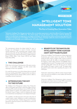
© Copyright 2026