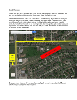
Applied Mechanics and Materials Vols. 670-671 (2014) pp 1330-1336
© (2014) Trans Tech Publications, Switzerland
doi:10.4028/www.scientific.net/AMM.670-671.1330
Submitted: 24.07.2014
Accepted: 03.08.2014
Control method for vehicles on base of natural energy recovery
Viacheslav Pshikhopov1, a, Mikhail Medvedev2,b and Anatoly Gaiduk3,c
1
Russian Federation, Taganrog, 347928, Ovrazniy, 6a
2
Russian Federation, Taganrog, 347900, Lomakina, 110, app. 51
3
Russian Federation, Taganrog, 347900, Slesarnaya, 26, app. 2
a
b
c
[email protected], [email protected], [email protected]
Keywords: Control method, vehicle, energy recovery, position-path control.
Abstract. This paper is devoted to vehicle movement control method based on the natural energy
recovery [1] and position-path control approach [2,3,4]. This method ensures the fullest use of
kinematic energy of the controlled vehicle. Method is applied for path profile with variable height.
Vehicle velocity is changed to minimize kinematic energy losses. The time of the path passage is
accounted in the designed method. In this report typical profiles of the controlled vehicle are
considered. In general case the vehicle velocity program is developed on base of solutions for typical
profiles. The vehicle velocity program is changing while vehicle is moving. The developed method is
applied for control of trains implemented with electrical power drives. On base of train model
studying it is proved that optimal mode of trains acceleration is maximal traction. The maximal
traction ensures minimum energy consumption of train drives. But the traction of trains is extreme
function of the speed wheel slip [5, 6]. Therefore the new extreme control for the train drives is
developed. This method supports trains traction in extreme value. The developed method is
implemented in simulator based on Matlab and Universal Mechanism. Movement of a freight train on
a real track section is simulated.
Introduction
Usually control of vehicles movement is planned to ensure constant vehicle speed. Usually if path is
not horizontal then the average speed is less than the maximal speed for the given vehicle. Due to
constant vehicle speed the vehicle thrust is increased when driving on the rise. But deceleration occurs
when driving downhill. Thus if assuming reduction in speed when driving on the rise then the
subsequent movement downhill speed can be increased at lower energy costs. Decreasing the energy
costs is able due to better utilization of the vehicle kinetic energy.
Energy Saving Movement Planning
Consider the quantitative relations, which can occur when the natural recovery. Let us consider
energy effect from the natural recovery.
Assume that path profile is known. For example consider the path profile from point A to point B
shown on fig. 1. There is a hill on the way from point A to point B. Parameters of the hill are altitude
h 1 m, and altitude h 2 m. The main peculiarity of the hill is h 2 < h 1 . The rest of the path is
horizontal. Assume that average vehicle speed V0 is known. Average vehicle speed V0 is calculated
on base of traveling time from point A to point B.
It is necessary to calculate speed V2, speed V3, distance Sy, and acceleration α . For the given profile
we obtain
V2 = V02 − 2 gh 1 .
(1)
0,5mV02 − mgh 1> 0 .
(2)
All rights reserved. No part of contents of this paper may be reproduced or transmitted in any form or by any means without the written permission of TTP,
www.ttp.net. (ID: 80.250.181.144-06/10/14,07:10:17)
Applied Mechanics and Materials Vols. 670-671
V3 = V02 − 2 g h 2 .
Sy =
α=
1
[V0 (2S3 − S1 − S2 ) − V2 (S3 − S1 ) − V3 ( S3 − S2 )] .
(V0 − V3 )
1
[3V02 − 4V0V3 + V32 ] .
2S y
1331
(3)
(4)
(5)
Herein g is gravity acceleration, m is a mass of vehicle.
Fig. 1 Path profile, speed, and thrust of vehicle
Similar expressions are obtained for other profiles.
Consider the next example: S1=2000 m, S2=2300 m, S3=2500 m, h1=20 m, h2=12 m, V0=25 m/s,
g=10 m/s2. It is necessary to calculate distance Sy, and acceleration α so that both average vehicle
speed as well as vehicle speed at point S3 are equal to V0.
1. From expression (1) and (3) we obtain: V2 = 15 m/s, V3=19,62 m/s. Thus vehicle speed
decreasing is V0-V3=5,38 m/s.
2. From (4) we obtain distance Sy=1129 m.
3. From (5) we obtain the acceleration required 0,131 m/s2.
4. Therefore the point of vehicle acceleration start is: Soa=S2-Sy=2300-1129=1171 m.
Thus to maintain the given average vehicle speed it is necessary for the point Soa increase thrust to
give the vehicle acceleration equal 0,131 m/s2. This acceleration is constant from point Soa to point
S2. At the the top of the hill a vehicle thrust is reduced to the value given by movement on the
horizontal path with speed 25 m/s.
Let us evaluate energy saving followed from vehicle moving with variable speed.
If vehicle speed is constant for path presented on the fig. 1, then additional energy for vehicle
climbing to 20 meters is
E12=mgh1= 200m Nm.
In addition the energy required to braking vehicle is
(6)
Е23 = mg(h1-h2) = 80m Nm.
(7)
Assume that 50 % of this energy is provided by the work of the motion resistance forces. Another
50 % of this energy is provided by active breaking. Therefore the complete additional energy costs for
the given example is 240m Nm.
If vehicle speed is variable for path presented on the fig. 1, then additional energy for vehicle
climbing to 20 meters is
Еad=mgh2=120m Nm.
Thus energy efficiency of the developed method for the given example is
(8)
1332
Applied Mechanics, Materials and Manufacturing IV
ηэк =
240m − 120m 120
=
= 0,5 .
240m
240
(9)
Extreme Control for Electrical Traction Train
On the base of proposed method it is possible to develop power saving control system for electrical
traction train.
Consider the equation of train movement
(
)
Vtr = Ftrac − Fmr 0 − Fmr1Vtr − Fmr 2Vtr2 / m .
(10)
Herein Fmr0 , Fmr1 , Fmr 2 are constants depending from train parameters and weight, Ftrac is
traction of train, Vtr is speed of train.
A first approximation of a train resistance force is quadratic function of train speed. This force is
[1]:
Fmr (Vtr ) = Fmr 0 + Fmr 1Vtr + Fmr 2 (Vtr ) 2 .
If train traction is constant then train speed for horizontal path in the steady state mode is
(11)

Fmr1 
4F 2
 −1 + 1 + mr
(
F
−
F
)
(12)
trac,max
mr0  .
2

2 Fmr2 
F
mr1


From (12) it is clear that train speed in the steady state mode is determined by the difference
between the maximum possible traction force Ftrac,max and the trait moving off resistance force Fmr0 .
Vtr∗ =
If Ftrac is constant then equation (7) takes the form
Vtr = f (Vtr )2 + gVtr + h .
(13)
Herein f = − Fmr 2 / m , g = − Fmr1 / m , h = ( Ftrac − Fmr 0 ) / m are constant.
Equation (8) is Riccati equation. If f ≠ 0 then for constant coefficients solution of equation (8) is:
C[exp( p2t ) − exp( − p1t )]
.
[C1 exp( − p1t ) + C2 exp( p2t )]
F
a
p 1 = Fmr1 (1 + 1 + a ) / 2m
,
Herein C = mr1
4 Fmr 2 1 + a
(14)
Vtr (t ) =
,
p 2 = Fmr1 (−1 + 1 + a ) / 2m
,
2
a = 4 Fmr2 ( Ftrac − Fmr0 ) / Fmr1
.
From investigation of solution (14) it is clear that for constant traction train energy costs is
2


Fmr0
mVc,tr
Qc (Vc,tr ) =
=
(15)
1 +
.
2( Ftrac − Fmr0 )
2  Ftrac − Fmr 0 
From (10) it is clear that the most power saving acceleration of train is the acceleration by maximal
traction. In other side traction of train is linear function of the friction coefficient kfr (Vsl ) . But
2
Ftrac mVc,tr
kfr (Vsl ) is extreme function of slipping speed Vsl . Maximum of the adhesion force is corresponding
to optimal value of slipping speed Vsl . Thus the most power saving mode oft rain acceleration is
acceleration with optimal slipping speed Vsl* .
Applied Mechanics and Materials Vols. 670-671
1333
Necessary condition of the adhesion force Fad extreme value is
dFad / dVsl = 0 .
(16)
Extreme value of the slipping speed Vsl* can be calculated on base of measuring the acceleration of
train wheels, acceleration of train, and the time rate of change of the traction motor. But errors of train
wh , acceleration of train Vtr , and the time rate of change of the traction motor
wheels acceleration ω
M calculation cause unacceptable large error of the derivative V calculation. Practically the errors
sl
dr
*
of measurements do not allow calculate value of Vsl correctly.
Therefore to calculate the extreme value of Fad we used method based on comparison differences
of the extreme function with its argument [7].
In the developed train control system the rising differences are used. These rising differences are
∆Fad,k = Fad,k − Fad,k −1 .
(17)
∆Vsl,k = Vsl,k − Vsl,k −1 .
(18)
∗
Symbol k is discrete time. Symbol k is time of the maximal value Fad ,max of the adhesion force
Fad . If k ≤ k ∗ then sign of the difference ∆Fad,k (17) and sign of the difference ∆Vsl,k (18) are same.
If k > k ∗ then sign of the difference ∆Fad,k (17) and sign of the difference ∆Vsl,k (18) are different. In
other words slipping speed is optimal if product ∆Fad,k ⋅ ∆Vsl,k changes sign.
Therefore we can propose the new method of detecting and supporting the extreme value of train
slipping speed. Assume that train is moving due to initial voltage applied to motors. Control system
measures slip speed and adhesion force and calculates differences ∆Fad,k (17) and ∆Vsl,k (18).
Extreme algorithm starts from time ks . The extreme algorithm is:
um,k = um,k −1 + u∆ sign (∆Fad,k −1 ) ⋅ sign (∆Vsl,k −1 ) , k = k s , k s + 1, k s + 2, ... .
(19)
Herein u∆ is positive constant (trial motion). Usually value of the trial motion u∆ is determined
by experiments.
The effectiveness of this method was carried out by computer simulation equations trains in
MATLAB. To reduce the time slicing effect we used averaged over several periods of the variables.
On fig. 2 we can see graph of voltage on the test locomotive engines. On fig. 3 we can see graph of
slip speed on the test locomotive. On fig. 2 and fig. 3 the trial motions are shown good. The trial
motions are changing the voltage on the motor and changing the slip speed. From fig. 3 it is clear that
the slip speed first is approaching the optimal value. Thereafter the slip speed is oscillating in the
neighborhood of the optimal value.
Fig. 2 Graph of voltage
1334
Applied Mechanics, Materials and Manufacturing IV
Fig. 3 Graph of slip speed
Simulation Complex
Simulation complex is based on complex for modeling and trials used at [2, 3, 8, 9, 10, 11]. This
complex was adapted by including program “Universal Mechanism”. Universal Mechanism allows
modeling detiled mechanics of trains. The block diagram of the developed complex is presented on
fig. 4.
User interface
Calculation of train speed
Numerical modeling unit
Control
system unit
Electrical
part unit
Path model
Train model
Modeling results analysis unit
User interface
Graph unit
3-D animation
Fig. 4 Block diagram of the modeling complex
On base of presented on fig. 4 complex energy effectiveness of the proposed method is checked.
On fig. 5 profile of section from 1785 km to 1777 km of path Tuapse – Armavir is shown. The section
length is about 8 km. The maximal train speed is 47 km/h.
Applied Mechanics and Materials Vols. 670-671
1335
Fig. 5 Profile of the path section
For the given path profile energy effect of the developed method is about 5 %. If path profile
consists of hills and dells, then power saving effect increases.
Summary
Proposed method can be used for another types of vehicles because dynamics model of the vehicles is
not used to calculate speed reference. But it is necessary account peculiarities of the vehicle. For
example power saving control of airship needs model of aerodynamics and wind model. [12, 13]. If
we have detailed information about vehicle model, then position path adaptive or robust control can
be used [4, 14].
Acknowledgements
This work was financially supported by the grant of Russian Education and Science Ministry “Theory
and methods of position path control for robotics systems in extreme modes and uncertain
environments”, the grant of Southern Federal University “Theory and method of power saving control
for distributed systems of energy generation, transmission, and consumption”, the grant of Russian
Foundation of Basic Research 13-08-00315, the grants of Russian President Council
MD-1098.2013.10 and NS-3437.2014.10.
References
[1] A.A. Zarifian, P.G. Kolpahchyan, V.Kh. Pshikhopov, M.Yu. Medvedev, N.V. Grebennikov,
V.V. Zak. Evaluation of electric traction’s energy efficiency by computer simulation, 2013
IMACS World Congress. 26-28, August, 2013. Barcelona.
[2] Pshikhopov V., Medvedev M., Kostjukov V., Fedorenko R., Gurenko B., Krukhmalev V. Airship
autopilot design. SAE Technical Papers. October 18-21, 2011. doi: 10.4271/2011-01-2736.
[3] Pshikhopov V. Kh., Medvedev M. Y., and Gurenko B. V. Homing and Docking Autopilot Design
for Autonomous Underwater Vehicle. Applied Mechanics and Materials Vols. 490-491 (2014). Pp.
700-707. Trans Tech Publications, Switzerland. doi:10.4028/www.scientific.net/AMM.
490-491.700.
[4] Medvedev M. Y., Pshikhopov V.Kh., Robust control of nonlinear dynamic systems. Proc. of
2010 IEEE Latin-American Conference on Communications. September 14 – 17, 2010, Bogota,
Colombia. ISBN: 978-1-4244-7172-0.
[5] Hill R.J. Electric railway traction. Traction drives with three–phase induction motors. Power
Engineeing Journal, 1994.- Vol. 3. Pp. 143-152.
1336
Applied Mechanics, Materials and Manufacturing IV
[6] Kalker J.J. Rolling contact phenomena: linear elasticity. Reports of the Department of applied
mathematical analysis. Delft, 2000.
[7] Rastrigin L. A. Systems of the extreme control. Мoscow, Nauka, 1974.
[8] Pshikhopov, V.Kh., Krukhmalev, V.A., Medvedev, M.Yu., Fedorenko, R.V., Kopylov, S.A.,
Budko, A.Yu., Chufistov, V.M. Adaptive control system design for robotic aircrafts. Proceedings
– 2013 IEEE Latin American Robotics Symposium, LARS 2013 PP. 67 – 70. doi:
10.1109/LARS.2013.59.
[9] Pshikhopov, V.Kh., Medvedev, M.Yu., Gaiduk, A.R., Gurenko, B.V. Control system design for
autonomous underwater vehicle. Proceedings – 2013 IEEE Latin American Robotics Symposium,
LARS 2013 PP. 77 – 82. doi: 10.1109/LARS.2013.61.
[10] Pshikhopov, V., Medvedev, M., Gaiduk, A., Neydorf, R. , Belyaev, V., Fedorenko, R.,
Krukhmalev, V. Mathematical model of robot on base of airship. 2013 Proceedings of the IEEE
Conference on Decision and Control, Pp. 959-964
[11] Pshikhopov, V.Kh., Medvedev, M., Gaiduk, A., Belyaev, V., Fedorenko, R., Krukhmalev, V.
Position-trajectory control system for robot on base of airship. 2013 Proceedings of the IEEE
Conference on Decision and Control, Pp. 3590-3595.
[12] Pshikhopov, V., Krukhmalev, V., Medvedev, M., Neydorf, R. Estimation of energy potential for
control of feeder of novel cruiser/feeder MAAT system, 2012, SAE Technical Papers, Vol 5.
[13] Pshikhopov, V., Medvedev, M., Neydorf, R., Krukhmalev, V., Kostjukov, V., Gaiduk, A.,
Voloshin, V. Impact of the feeder aerodynamics characteristics on the power of control actions in
steady and transient regimes. SAE 2012 Aerospace Electronics and Avionics Systems
Conference, 2012, Vol. 5.
[14] Pshikhopov, V., Medvedev, M. Block design of robust control systems by direct Lyapunov
method. 18th IFAC World Congress, Volume 18, Issue PART 1, 2011, Pages 10875-10880.