
Synergistic Co-processing of Red Mud mining waste and
Synergistic Co-processing of Red Mud mining waste and alkaline Black Liquor from the Pulp and Paper Industry by Christopher Francis George Gissane A Thesis presented to The University of Guelph In partial fulfillment of requirements for the degree of Master of Science in Chemistry Guelph, Ontario, Canada © Christopher Gissane, April, 2015 ABSTRACT SYNERGISTIC CO-PROCESSING OF RED MUD MINING WASTE AND ALKALINE BLACK LIQUOR FROM THE PULP AND PAPER INDUSTRY Christopher Francis George Gissane University of Guelph, 2015 Advisor: Professor Marcel Schlaf This thesis focused on the explorative study of synergistically co-processing Red Mud and Black Liquor under varying temperatures, pressures, reaction times, and material ratios. The goal being to generate a treated Red Mud with a substantially lower pH and increased carbon content that would be more environmentally tolerable and allow for the consideration of using the treated material as a viable soil additive and/or allow for the remediation and revegetation of Red Mud storage sites. Using a factorial design of experiments approach the study identified the most influential reaction parameters affecting the monitored responses. By applying a central composite design to those results, the optimum reaction conditions to achieve the desired results for pH, carbon content and several other characteristics were realized. Additionally, the design and construction of a unique explosion resistant high pressure hydrogenation laboratory was also undertaken as part of this thesis. To my Mom and Dad iii ACKNOWLEDGEMENTS First, I would like to thank my advisor, Dr. Marcel Schlaf. I am very grateful of the opportunities that you have given me as both a graduate and an undergraduate student. The last two years have definitely have been a test of patience for the both of us getting the new laboratory completed but I am grateful you trusted me to take the lead on the project. That opportunity allowed me to gain experience and learn from mistakes that few in my position ever get the chance to do. You have taught me to look at the world with a more analytical mindset and it has been a privilege to work for you and alongside you. Special thanks to everyone in the electronics and machine shops, especially Ian, Steve, and Case, for all of their help with the various aspects of the projects. I am appreciative to the many members of the Schlaf group I have had the pleasure to know, as well as to my friends throughout the department, for all of their support. I was fortunate enough to have worked alongside a number of highly talented chemists, all of whom assisted me to improve my skills every day. I can only hope that my future endeavors bring workplace dynamics as memorable and rewarding as those I have enjoyed here. Last, though far from least, I would like to thank my friends and family. I am very fortunate to have such a select group of people in my life that showed such interest in my work and helped me in so many ways over the years and to listen to my ranting over all the issues that kept cropping up. iv Table of Contents 1 1.1 INTRODUCTION.............................................................................................................................. 1 Motivation .......................................................................................................................................................1 1.2 Aluminium Industry .......................................................................................................................................2 1.2.1 The Bayer Process ........................................................................................................................................2 1.2.2 Red Mud Waste ............................................................................................................................................4 1.2.2.1 Disposal Techniques and Environmental Issues ..................................................................................4 1.2.2.2 Multi-Functional Catalyst Potential .....................................................................................................6 1.3 Pulp and Paper Industry ................................................................................................................................7 1.3.1 Lingocellulosic Biomass ..............................................................................................................................7 1.3.1.1 Cellulose ..............................................................................................................................................8 1.3.1.2 Hemicellulose ......................................................................................................................................8 1.3.1.3 Lignin ..................................................................................................................................................9 1.3.2 Major Pulping Processes15,16 ...................................................................................................................... 13 1.3.2.1 Kraft Pulping ..................................................................................................................................... 13 1.3.2.2 Sulfite Pulping ................................................................................................................................... 14 1.3.2.3 Soda Pulping ..................................................................................................................................... 15 1.3.3 Black Liquor Waste.................................................................................................................................... 17 1.3.3.1 Composition and Properties .............................................................................................................. 17 1.3.3.2 Disposal Techniques.......................................................................................................................... 19 1.4 Overview of Projects .................................................................................................................................... 21 1.4.1 Project I: Design and Construction of the High Pressure Hydrogenation Lab ........................................... 21 1.4.2 Project II: Neutralization of Red Mud using Strong Black Liquor as a reagent ......................................... 22 2 2.1 RESULTS AND DISCUSSION – PROJECT I .............................................................................. 23 Infrastructure Design Features ................................................................................................................... 23 2.2 High Pressure Reactors ................................................................................................................................ 27 2.2.1 Reactor Installation and Validation ............................................................................................................ 29 2.2.2 Comparison of Temperature and Pressure Response to Theoretical Values using NIST software ............ 30 3 3.1 RESULTS AND DISCUSSION – PROJECT II............................................................................. 34 A Counterintuitive Approach ...................................................................................................................... 35 3.2 24 Factorial Design ........................................................................................................................................ 37 3.2.1 Initial Observations .................................................................................................................................... 41 3.2.1.1 pH of Black Liquor in storage ........................................................................................................... 41 3.2.1.2 Precipitate formation from the aqueous liquid phase ........................................................................ 42 3.2.1.3 pH values ........................................................................................................................................... 45 3.2.1.4 Coloured aqueous phase .................................................................................................................... 46 v 3.2.1.5 Recovered Solid Phase ...................................................................................................................... 48 3.2.2 Significant Factors and Interactions ........................................................................................................... 50 3.2.2.1 pH of Solid Phase .............................................................................................................................. 52 3.2.2.2 pH of Aqueous Phase ........................................................................................................................ 53 3.2.2.3 Mass of Aqueous Phase ..................................................................................................................... 54 3.2.2.4 Carbon Content of Solid Phase .......................................................................................................... 54 3.2.2.5 Water Content of Aqueous Phase ...................................................................................................... 55 3.2.2.6 Magnetic Susceptibility ..................................................................................................................... 55 3.2.2.7 Sodium Concentration in the Solid Phase ......................................................................................... 56 3.2.2.8 Summary ........................................................................................................................................... 57 3.3 Central Composite Design ........................................................................................................................... 58 3.3.1.1 pH of Solid Phase .............................................................................................................................. 60 3.3.1.2 pH of Aqueous Phase ........................................................................................................................ 63 3.3.1.3 Mass of Aqueous Phase ..................................................................................................................... 64 3.3.1.4 Carbon Content of Solid Phase .......................................................................................................... 64 3.3.1.5 Water Content of Aqueous Phase ...................................................................................................... 65 3.3.1.6 Magnetic Susceptibility ..................................................................................................................... 65 3.3.1.7 Sodium Concentration in Red Mud ................................................................................................... 65 3.3.1.8 Statistical relevance of the data ......................................................................................................... 66 3.3.2 Optimum Reaction Conditions ................................................................................................................... 67 3.3.3 Summary .................................................................................................................................................... 69 3.4 Experimental ................................................................................................................................................. 71 3.4.1 Factorial Design Calculations .................................................................................................................... 71 3.4.2 General Procedure for Co-processing Reactions ........................................................................................ 72 3.4.3 Analytical Instrumentation ......................................................................................................................... 73 4 SUMMARY OF RESULTS ............................................................................................................. 75 REFERENCES.......................................................................................................................................... 77 APPENDIX............................................................................................................................................... 79 Appendix A: Select Micro-GC Traces ..................................................................................................................... 80 A1: Micro-GC trace of 1000ppm C1 – C6 alkane standards................................................................................... 81 A2: Micro-GC trace of 1000 ppm C2 – C6 alkene standards.................................................................................. 81 A3: Micro-GC trace of lab atmosphere reference ................................................................................................... 82 A4: Micro-GC trace of DoE reaction, representative over all reactions conducted ................................................ 82 A5: Micro-GC trace of acid digestion white precipitate recovered from aqueous phase post- reaction using 2M HCl (representative of all applicable reactions) ...................................................................................................... 83 Appendix B: 3D Autogenic Pressure Response as a Function of Time and Temperature for Multi-Reactor System and REFPROP Water Vapour Pressure Plots ........................................................................................... 84 B1: Bach autogenic pressure response as a function of time and temperature with 50, 100 and 150mL of water .. 85 B2: Escher autogenic pressure response as a function of time and temperature with 50, 100 and 150mL of water ................................................................................................................................................................................. 86 vi B3: Gödel autogenic pressure response as a function of time and temperature with 50, 100 and 150mL of water 87 B4: Theoretical Pressure-Temperature Response for Water vapour contained in an ideal closed system within the range of the High Pressure Reactor specifications. ................................................................................................. 88 B5: Theoretical pressure-temperature response for water vapour contained in an ideal closed system near the limits of the high pressure reactor specifications. ................................................................................................... 89 Appendix C: Spectral data for aqueous phases ...................................................................................................... 90 C1: 1H NMR of red aqueous phase obtained on a 400 MHz spectrometer using D 2O as the solvent. .................... 91 C2: 1H NMR of red aqueous phase obtained on a 400 MHz spectrometer using D2O as the solvent and water suppression NMR program. .................................................................................................................................... 92 C3: 13C NMR of red aqueous phase obtained on a 400 MHz spectrometer using D 2O as the solvent .................... 93 C4: 1H NMR of purple aqueous phase obtained on a 400 MHz spectrometer using D 2O as the solvent ................ 94 C5: 1H NMR of purple aqueous phase obtained on a 400 MHz spectrometer using D2O as the solvent and water suppression. ............................................................................................................................................................. 95 C6: 13C NMR of purple aqueous phase obtained on a 400 MHz spectrometer using D 2O as the solvent ............... 96 Appendix D: Pareto charts, residual plots, main effects plots, interaction plots, and cube plots from DoE analysis ....................................................................................................................................................................... 97 24 Factorial Design .................................................................................................................................................. 98 D1: Pareto chart, residual plot, main effects plot, interaction plot, and cube plot for pH of solid phase before (Top) and after (Middle) reduction of terms for calculation ............................................................................... 98 D2: Pareto chart, residual plot, main effects plot, interaction plot, and cube plot for pH of aqueous phase before (Top) and after (Middle) reduction of terms for calculation ............................................................................... 99 D3: Pareto chart, residual plot, main effects plot, interaction plot, and cube plot for mass of aqueous phase before (Top) and after (Middle) reduction of terms for calculation .................................................................. 100 D4: Pareto chart, residual plot, main effects plot, interaction plot, and cube plot for carbon content of solid phase before (Top) and after (Middle) reduction of terms for calculation ........................................................ 101 D5: Pareto chart, residual plot, main effects plot, interaction plot, and cube plot for water content of aqueous phase before (Top) and after (Middle) reduction of terms for calculation ........................................................ 102 D6: Pareto chart, residual plot, main effects plot, interaction plot, and cube plot for magnetic susceptibility before (Top) and after (Middle) reduction of terms for calculation .................................................................. 103 D7: Pareto chart, residual plot, main effects plot, interaction plot, and cube plot for sodium concentration in the solid phase before (Top) and after (Middle) reduction of terms for calculation .............................................. 104 Central Composite Design .................................................................................................................................... 105 D8: Residual plot, Contour plots, and response surface plots for pH of solid phase ........................................ 105 D9: Residual plot, Contour plots, and response surface plots for the pH of aqueous phase ............................. 106 D10: Residual plot, Contour plots, and response surface plots for the mass of aqueous phase ........................ 107 D11: Residual plot, Contour plots, and response surface plots for the carbon content of solid phase .............. 108 D12: Residual plot, Contour plots, and response surface plots for the water content of aqueous phase........... 109 D13: Residual plot, Contour plots, and response surface plots for the magnetic susceptibility ........................ 110 D14: Residual plot, Contour plots, and response surface plots for the sodium concentration in the solid phase .......................................................................................................................................................................... 111 D15: Optimized reaction parameters predicted by Minitab®’s response optimizer ......................................... 112 D16: Overlaid contour plots of response factors highlighting the optimum results while holding reaction time fixed at 0.5 hrs (Top), 1.75 hrs (Middle), and 3 hrs (Bottom) .......................................................................... 113 Appendix E: SOP for High Pressure Reactors ...................................................................................................... 114 vii Appendix F: Gas Sensor Alarm Response Procedures and Hydrogenation Lab Information distributed to EHS, Physical Resources and Campus Police/Fire Dispatch Centre .................................................................. 126 viii List of Charts Chart 2-1: High temperature range vs. pressure plots for water validation experiments and NIST prediction calculations .................................................................................................................. 33 ix List of Figures Figure 1-1: Illustration of alumina refining using the Bayer Process 3........................................... 2 Figure 1-2: Representation of cellulose polymer and glucose repeating units ............................... 8 Figure 1-3: Representation of hemicellulose polymer with repeating xylose units and other possible sugar monomers. ............................................................................................................... 9 Figure 1-4: Representations of Lignin monomers .......................................................................... 9 Figure 1-5: Example of branched lignin structure within lignocellulosic biomass14.................... 10 Figure 1-6: Chemical structures of common turpentine components ........................................... 18 Figure 2-1: Watchtower control screen for multi-reactor system ................................................. 29 Figure 3-1: Pictures of the coloured aqueous phases recovered from various reactions. Examples of the darken colours (Top), dark red (Top Left), rusty red (Top Middle), dark purple (Top Right); observed darkening of coloured solution during reaction workup (Bottom), initial colour (Bottom Left), after five minutes (Bottom Right) ........................................................................ 48 x List of Schemes Scheme 1-1: Extraction of aluminium hydroxide compounds by addition of sodium hydroxide .. 3 Scheme 1-2: Precipitation Process .................................................................................................. 3 Scheme 1-3: Calcination Process .................................................................................................... 3 Scheme 1-4: Formation of sulfite pulping liquor 1,18 .................................................................... 14 Scheme 1-5: Proposed α-aryl bond cleavage under alkaline pulping conditions ......................... 16 Scheme 1-6: Examples of reactions within the Recovery Boiler ................................................. 20 Scheme 1-7: Example of the Reconstitution of Pulping Chemicals ............................................. 20 Scheme 3-1: Formation pathway for sodium carbonate in situ. ................................................... 44 Scheme 3-2: Formation of pathway of carbonic acid and sodium bicarbonate in situ. ................ 44 Scheme 3-3: Decomposition pathway of sodium bicarbonate into sodium carbonate when heated. ....................................................................................................................................................... 44 Scheme 3-4: Proposed hydrogen gas reaction with iron species in Red Mud. ............................. 53 xi List of Tables Table 1-1: General composition of Red Mud.9 ............................................................................... 7 Table 1-2: Examples of the seven bonding motifs between lignin repeating units.15................... 12 Table 1-3: Sulfite reaction conditions.18 ....................................................................................... 15 Table 2-1: Description of hydrogenation laboratory hazardous environment classification.25,26 . 23 Table 2-2: Gas Sensor Alarm Set points ....................................................................................... 26 Table 3-1: Properties of supplied Red Mud. ................................................................................. 34 Table 3-2: Properties of supplied Black Liquor. ........................................................................... 35 Table 3-3: Main factors chosen for Factorial Design study and selected settings. ....................... 38 Table 3-4: Response Factors chosen for the analysis of reaction products. ................................. 40 Table 3-5: Reaction parameters for Factorial Design. .................................................................. 40 Table 3-6: Peak area comparison of gas samples from the Black Liquor storage bucket and the laboratory atmosphere. .................................................................................................................. 42 Table 3-7: Peak area comparison of gas samples from acid digestion of solid phase. ................. 43 Table 3-8: Identification of reactions producing a precipitate that could be isolated. .................. 43 Table 3-9: Average pH of solid phase and aqueous phase samples dependant on if the reaction produced a precipitate. .................................................................................................................. 45 Table 3-10: Mass, water content, and pH of aqueous phases; mass, pH values, carbon content and magnetic susceptibility of solid phases and degree of reactor coking observed. ................... 49 Table 3-11: Linear regression results and significant effects of regression coefficients from the 24 factorial design in coded units. ..................................................................................................... 51 Table 3-12: Reaction parameters for Central Composite Design. (cf. Table 3-5 for actual values of +/0/-). ........................................................................................................................................ 58 Table 3-13: Mass, water content, and pH of aqueous phases, pH values, carbon content, and magnetic susceptibility of solid phases. ........................................................................................ 59 Table 3-14: Experimental model fitted to the responses from the 17 reactions in Table 3-12 with uncoded factors. ............................................................................................................................ 62 Table 3-15: Analysis of variance for the response factors for the neutralization of Red Mud using Strong Black Liquor. ..................................................................................................................... 62 Table 3-16: Comparison of optimum reaction conditions between response optimizer function and overlaid contour plots. ............................................................................................................ 68 xii Glossary of Abbreviations AAS Atomic Absorbance Spectroscopy AE Parker Autoclave Engineers BL Black Liquor Coeff. coefficient DoE Design of Experiments EHS Environmental Health and Safety EOS Equation of State ESD Electrostatic Discharge ft. lbs. foot-pounds FPT Fire Prevention Team GC gas chromatography LDPI Luminaire Design for Performance and Innovation M mole/litre (Molarity) MFM Mass flow meter NIST National Institute of Standards and Technology NMR Nuclear Magnetic Resonance (spectroscopy) OCC Original corrugated cardboard ppm parts per million RM Red Mud rpm revolutions per minute rxn reaction SSC Summerlee Science Complex T316 SS type-316 Stainless Steel T.E.L. Temperature Electronics Ltd WGSR Water-gas shift reaction wt. by weight XRF X-ray fluorescence xiii 1 Introduction 1.1 Motivation Waste management is a crucial operation, especially for large scale industrial operations. The capital expenditures and possible liabilities associated with waste disposal can quickly become a financial and environmental burden for companies in a various industries. Two such industries facing immediate waste issues are the Pulp and Paper Industry which produces a waste material referred to as Black Liquor on a scale of up to 7 tonnes per tonne of useful pulp and the Alumina Refining Industry which produces Red Mud as a by-product on a scale of 2 tonnes per tonne of alumina.1,2 These waste materials are generated on an impressively large scale, but storage of them is becoming a major problem especially in the case of Red Mud; current strategies using lagoons and other long term storage methods are quickly becoming unfeasible, both economically and environmentally. Methods must be developed that utilize the wastes generated from these streams. This would negate the need for long term storage options and possibly produce products that are in some way useful to other industries. Such products could be beneficial as they may add an additional revenue generating stream to outset the processing costs. If not, the products could be at least more environmentally tolerable and thus be disposed of without the threat of damaging the environment or causing a legal and financial liability for the companies and industries as a whole in years to come. 1 1.2 Aluminium Industry 1.2.1 The Bayer Process Red Mud, the technical name being bauxite residue, is a waste product of the industrial refining process known as the Bayer Process used to produce pure alumina (Al2O3) from Bauxite ore. Bauxite is composed of a multitude of metal oxides including a high percentage of aluminum hydroxide and oxide minerals which is the reason for its use as the raw starting material in the refining to alumina powder. The Bayer process consists of four main steps: Digestion, Clarification, Precipitation, and Calcination (Figure 1-1). The bauxite is prepared for the digestion stage by milling the ore into smaller particles to increase the reaction surface area before being combined with an aqueous sodium hydroxide solution. Figure 1-1: Illustration of alumina refining using the Bayer Process 3 Exploiting the amphoteric nature of Al3+ ions, the sodium hydroxide extracts many of the multiple forms of aluminum hydroxide compounds (Al(OH)3 and AlO(OH)), mostly found in the forms of Gibbsite, Böhmite, and Diaspore, out of the bauxite as water soluble tetrahydroxyaluminate(III) ions ([Al(OH)4]-) (Scheme 1-1). 2 Alkaline digestion of Gibbsite + − 𝐴𝑙(𝑂𝐻)3(𝑠) + 𝑁𝑎(𝑎𝑞) + 𝑂𝐻(𝑎𝑞) → 𝐻2 𝑂 + [𝐴𝑙(𝑂𝐻)4 ]− (𝑎𝑞) + 𝑁𝑎(𝑎𝑞) Alkaline digestion of Böhmite and Diaspore + − 𝐴𝑙𝑂(𝑂𝐻)(𝑠) + 𝑁𝑎(𝑎𝑞) + 𝑂𝐻(𝑎𝑞) + 𝐻2 𝑂 → 𝐻2 𝑂 + [𝐴𝑙(𝑂𝐻)4 ]− (𝑎𝑞) + 𝑁𝑎(𝑎𝑞) Scheme 1-1: Extraction of aluminium hydroxide compounds by addition of sodium hydroxide Once the extraction is complete, the aqueous slurry is pumped into raking thickeners where the suspended non-soluble metal oxides and other impurities are filtered or sedimented out, gathered and drained off into bauxite residue disposal areas.4 This material is classified as “Red Mud”, whose characteristic rusty red colour is that of the iron oxide hematite (Fe2O3) present in up to ~60% w/w. The remaining [Al(OH)4]- ion solution is pumped into the precipitation tanks where over the course of several days water is drawn off by evaporation, allowing the Al(OH)3 to crystallize out of solution. The crystallization process can be expedited by the addition of pure crystalline aluminum oxide seeds which can be recovered once the precipitation is complete and recycled for future use (Scheme 1-2). + [𝐴𝑙(𝑂𝐻)4 ]− (𝑎𝑞) + 𝑁𝑎(𝑎𝑞) → −𝐻2 𝑂 + − 𝐴𝑙(𝑂𝐻)3(𝑠) + 𝑁𝑎(𝑎𝑞) + 𝑂𝐻(𝑎𝑞) Scheme 1-2: Precipitation Process Once the precipitation has gone to completion, the precipitate is loaded into gas-fired kilns set to a temperature of >1100 ºC. The crystalline solid is fully dried resulting in a fine white powder product which is pure aluminum oxide (Al2O3) (Scheme 1-3).5 This powder can then be further electro-refined into pure aluminum metal ingots. ∆ 𝐴𝑙(𝑂𝐻)3(𝑠) → 𝐴𝑙2 𝑂3(𝑠) + 3 𝐻2 𝑂 Scheme 1-3: Calcination Process 3 1.2.2 Red Mud Waste 1.2.2.1 Disposal Techniques and Environmental Issues Several major issues arise when attempting to dispose of Red Mud. The primary issue is the quantity of Red Mud produced: in general roughly 2 tons of Red Mud is produced for every ton of alumina.2 Over the lifetime of the aluminum industry, which began with the display of a piece of pure aluminum at the World Fair in Paris in 1898 (at the time more valuable than Gold on w/w basis), this has resulted in an estimated current accumulation of ~3 billion tons of Red Mud worldwide with an additional ~120 million tons added every year at the current production rate.6 The secondary issue is the high alkalinity of the Red Mud (typically pH ≥12), which forces its classification as a hazardous waste and prevents its use, e.g., as an iron ore source or as a soil or cement additive. The main concern with Red Mud arises when discussing disposal. With such large production volumes, the disposal techniques are still fairly basic; three main methods of disposal exist: direct disposal into the ocean, containment in tailing ponds, and dry-stacking. A series of reviews by Klauber et. al.7 provide details on most of the advantages and disadvantages of the methods therefore only a brief overview will be presented. Direct ocean dumping is only used in areas where enough space for land disposal facilities simply does not exist or is too expensive to be viable (notably Japan and in the past Greece) and is rarely used today if at all due to environmental concerns. Certain bauxite sources contain harmful concentrations of transition or actinide metals such as chromium (Greece) or uranium (Australia), respectively, that can over time damage to the ecosystem and be detrimental to the long term viability of the local ecology. Tailing ponds were once the most popular form of disposal but due to the quantity of current production, the cost of large plots of land used for containment, and the environmental 4 and financial repercussions if containment were to fail this method is quickly becoming a poor option, both economically and ecologically. The final method is dry-stacking; the method involves spreading out Red Mud in thin layers and allowing partial evaporation of water to take place to create a more dense mixture before placing additional layers over top and repeating the process. At some locations, (AluGreece, Gulf of Corinth) this process is aided by first filterpressing the Red Mud to reduce its water content, while at the same time recovering more NaOH solution. An issue with this method is that fully dried Red Mud is a very fine powder with a particle sizes ranging from 160 µm to well below 40 µm.8 If the Red Mud dries, it can easily become airborne in a breeze which, due to its alkalinity, can be detrimental to a person’s health if for instance it comes in contact with the mucus membranes of the respiratory system. Therefore, the challenge becomes maintaining a minimum moisture content threshold in the mixture as not to allow the powder to fully dry and become airborne. As stated before, due to the addition of sodium hydroxide in the digestion stage of the Bayer process Red Mud typically has a pH ≥ 12.7 With such a high pH, many countries classify Red Mud as hazardous waste which complicates the disposal by making it much more expensive and difficult. To solve the disposal problem a solution needs to be found through which Red Mud can be treated effectively and efficiently to lower its pH and generate a substance that is no longer classified as hazardous and has the possibility for future applications elsewhere. The ideal situation would be for this treated Red Mud to represent an economic opportunity rather than liability, i.e., the transformation of a waste with an effectively negative value (due to storage and stewardship costs) into value-added metallurgical or otherwise usable resource. 5 1.2.2.2 Multi-Functional Catalyst Potential Red Mud consists of all metal oxides and minerals that were not soluble in the digestion of bauxite ore due to their formation of insoluble hydroxides, oxides and iso-polybases, notably [Fe(O)(OH)]n. Although the exact composition of Red Mud will vary wildly throughout all bauxite deposits worldwide, the general composition of particles expected to be present in the mixture is fairly consistent.9 This composition is highly complex; however, the compounds can be grouped by similar elemental content. Grouping the compounds in such a way allows for the establishment of groupings of known catalytically active compounds to become obvious as shown in Table 1-1. Iron (III) oxide (Fe2O3) derived suboxides such as magnetite (Fe3O4) and Wuestite (FeO) are known to be active as hydrogenation catalysts at elevated temperatures (T > 350 °C), while titanium oxide (TiO2) is a viable ketonization catalyst. Iron suboxide catalysts are also active for the water gas shift reaction and Fischer-Tropsch chemistry.10 Silicon and aluminum oxides (as SiO2 and Al2O3, respectively) are all known Brønstedt/Lewis acid/base catalysts often serving as catalyst supports for other metals. Finally, calcium and sodium oxides (CaO and Na2O respectively) can be viewed as potential modifiers and promoters in an overall catalytically active matrix.10,11 Intriguing considerations are that the occasional substitution of Al3+ with Fe3+ in this matrix could generate unique single atom defect sites that may be catalytically highly active and that the various components of Red Mud could act in a synergistic manner further enhancing its overall catalytic activity. Given that Red Mud is composed of such a large percentage of common catalysts allows for the consideration of using of the waste product as an extremely affordable catalyst; it can even be considered as a sacrificial catalyst – a deliberate contradiction in terms – given the large stockpile of Red Mud available globally. 6 Table 1-1: General composition of Red Mud.9 Element Fe Al Si Ti Ca Na Associated Minerals Hematite Goethite Magnetite Boehmite Gibbsite Diaspore Sodalite Cancrinite Quartz Rutile Anatase Perovskite Ilmenite Calcite Whewellite Tricalcium aluminate Sodalite Cancrinite Dawsonite Unit Cell Chemical Formula α-Fe2O3 α-FeOOH Fe3O4 γ-AlOOH γ-Al(OH)3 α-AlOOH Na6[Al6Si6O24]Cl2 Na6[Al6Si6O24]∙2[CaCO3]∙2H2O SiO2 TiO2 TiO2 CaTiO3 TiFeO3 CaCO3 CaC2O4∙H2O Ca3Al2(OH)12 Na6[Al6Si6O24]Cl2 Na6[Al6Si6O24]∙2[CaCO3]∙2H2O NaAl(OH)2∙CO3 1.3 Pulp and Paper Industry The Pulp and Paper Industry has existed for centuries. Throughout the years since its establishment, many different pulping processes have been developed and replaced or further refined as technology evolved and knowledge of the wood chemistry involved became more understood. However, the parts that have remained constant have been the feedstocks required. 1.3.1 Lingocellulosic Biomass The feedstocks utilized for pulp production depend on the pulping method in operation. Some methods can process multiple sources such as hardwoods, softwoods, and annual plants without issue while others are only useful for a select source of biomass. Whatever source is required they are all forms of lignocellulosic biomass. Lignocellulosic biomass is composed of three different polymers: cellulose, hemicellulose, and lignin; the ratio of the three polymers 7 varying greatly depending on the type of biomass but generally the composition percentages are 38-50% cellulose, 23-32% hemicellulose, and 10-30% lignin.12 1.3.1.1 Cellulose Cellulose is composed of D-glucose monomers linked together by β-1,4 glycosidic bonds that form long straight polymer strands. These strands are bound tightly together by intermolecular hydrogen bonding between the many hydroxyl groups present within glucose molecules as illustrated in Figure 1-2. The strands are generally between a hundred to ten thousand units long and as stated above constitute the majority of the plant cell wall structure.12 Figure 1-2: Representation of cellulose polymer and glucose repeating units 1.3.1.2 Hemicellulose The second most abundant polymer in lignocellulosic biomass, hemicellulose, is more complex than cellulose as the fibers are branched and are a combination of multiple different sugar monomers. There is less hydrogen bonding between strands due to the less ordered structure leading to a decrease in the density of the packed fibers; the fibers are also shorter than cellulose fibers, approximately only a few thousand units long or less. The fiber backbone is usually formed by mixed β-1,4 glycoside connected xylose monomers followed by interspersed and branched mannose, galactose, arabinose, and glucose throughout; the positioning and 8 number of these sugar monomers are dependent on the type of plant.12 Some types of hemicellulose also contain oxidized forms of the hexose sugars such as glucuronic acid as shown in Figure 1-3. Figure 1-3: Representation of hemicellulose polymer with repeating xylose units and other possible sugar monomers. 1.3.1.3 Lignin Lignin is the third component of lignocellulosic biomass which is formed from randomly repeating units of three different types of substituted phenols; trans-p-courmaryl alcohol, coniferyl alcohol, and sinapyl alcohol as shown in Figure 1-4, i.e., lignin is – strictly speaking – not a polymer, but better described as a macromolecule.12,13 Figure 1-4: Representations of Lignin monomers 9 These repeating units are bound together using seven types of bonding motifs involving carboncarbon bonds and ether bridges as shown in Table 1-2. The variability of the bonding arrangements within lignin facilitates the formation of a highly rigid compound that structurally supports and binds strands of cellulose and hemicellulose fibers together within plants. As Figure 1-5 demonstrates, the three-dimensional bonding of lignin can be complex and difficult to display in a single plane however it becomes obvious that due to the multitude of varying C-C and C-O-C cross-linkages lignin is a robust structural system that has evolved to protect the more easily damaged polymeric structures of plants. Figure 1-5: Example of branched lignin structure within lignocellulosic biomass14 Breaking lignin down into manageable units and effectively separating it from the more ordered structures of cellulose and hemicellulose without damaging them presents a major 10 challenge. The required chemical and/or catalytic treatment system would have to possess the ability to target and cleave a variety of bonding motifs in lignin and hemicellulose without attacking the bonding of cellulose which needs to be left as intact as possible. Such a system has yet to be developed and as such, the pulp and paper industry still relies on more brute force and harsh chemical systems, such as highly acidic or basic conditions, to forcibly breakdown the cross-linkages of lignin in order to separate the desired cellulose pulp from lignin and hemicellulose. 11 Table 1-2: Examples of the seven bonding motifs between lignin repeating units.15 Carbon Bonds Illustration of Bonding Motif Ether Linkages BetaBeta Alpha-O-4 Beta-1 Beta-O-4 Beta-5 4-O-5 5-5 12 Illustration of Bonding Motif 1.3.2 Major Pulping Processes15,16 Originally, the only available method of extracting pulp from wood was exclusively by mechanical movement of a stone grinding wheel against the pulp feedstock. This method provided high yields of pulp fibers but lacked the ability to separate the lignin from the cellulose fibers. This decreased the strength of the final paper product as the lignin interfered with the formation of hydrogen bond crosslinking between the fibers; the lignin also turned the paper yellow overtime when exposed to air and light.1 As knowledge and understanding of the interactions between industrial chemicals and the chemical structure of biomass increased so too did the dependence on chemical actions to breakdown and separate the cellulose and hemicellulose from lignin. The entirely mechanical methods were replaced over time by chemimechanical and semi-chemical, and eventually purely chemical processes became the established methods of pulping. The use of chemical based systems for processing pulp offered increased fiber strength in the final product as the lignin was successful separated from the cellulose fibers but at the cost of lower pulp yields. This is because the chemicals that dissolve lignin also dissolve and/or degrade hemicellulose and cellulose fibers.1 Today, the pulping industry relies heavily on chemical pulping processes and they account for the majority of the global production of pulp. The three main techniques are Kraft pulping, Sulfite pulping, and Soda pulping which constitute 80%, 10%, and 5% of the total pulp production, respectively.17,18 1.3.2.1 Kraft Pulping The Kraft Process, also referred to as the sulfate process, is by far the most utilized pulping method due to the efficiency of delignification, stronger fibers and shorter cooking time than other comparable methods. The method operates using both sodium hydroxide and sodium sulfide (Na2S) at pH ~13, with reaction temperatures between 160-180 ºC and a steam pressure 13 of 120 psi for approximately 30-180 minutes to dissolve the majority of lignin from the feedstocks; pulp yields are on the order of ~43% (w/w) for softwoods and ~50% (w/w) for hardwoods.1,19 The disadvantages associated with the Kraft process are lower yields compared to mechanical pulping due to chemical degradation of carbohydrates and possibly dangerous emissions due to the presence of sulphur dioxide in the flue gases from the chemical pulping digesters. 1.3.2.2 Sulfite Pulping Another fully chemical pulping process is Sulfite Pulping, which is a collection of several slightly different methods all requiring the use of sulfurous acid (H2SO3) and the corresponding alkali salts. The major processes are acidic bisulfite pulping, bisulfite pulping, neutral sulfite pulping, alkaline sulfite pulping as well as a multistage sulfite pulping process and an anthraquinone catalyzed process. All the processes require the essential use of sulfur dioxide and sulfurous acid to be successful in pulping the hardwood and softwood feedstocks. The sulfurous acid is generated by burning sulfur under controlled contact with oxygen to generate SO2 (instead of the fully oxidized form of SO3 the formation of which requires a V2O5 catalyst), which is then dissolved in water to form H2SO3. Upon the addition of a hydroxide salt, the acid reacts to form the corresponding sulfite salt and water as illustrated in Scheme 1-4; the required reaction conditions are shown in Table 1-3. 𝑆 + 𝑂2 → 𝑆𝑂2 𝑆𝑂2 + 𝐻2 𝑂 𝐻2 𝑆𝑂3 𝐻2 𝑆𝑂3 + 𝑀𝑂𝐻 𝑀𝐻𝑆𝑂3 + 𝐻2 𝑂 𝑀𝐻𝑆𝑂3 + 𝑀𝑂𝐻 𝑀2 𝑆𝑂3 + 𝐻2 𝑂 1 1 𝑊ℎ𝑒𝑟𝑒 𝑀 = 𝑁𝑎, 𝐾, 𝐶𝑎, 𝑁𝐻4 , 𝐶𝑎, 𝑜𝑟 𝑀𝑔 2 2 Scheme 1-4: Formation of sulfite pulping liquor 1,18 14 Table 1-3: Sulfite reaction conditions.18 Process pH range Acidic Bisulfite 1-2 Bisulfite 3-5 Temperature (ºC) Time (min) Pulp yield (%) SO2∙H2O, H+, HSO3- 125-143 180-420 40-50 H+, HSO3- 150-170 60-180 50-65 Base Cation Active ions Ca2+, Mg2+, Na+, NH4+ Mg2+, Na+, NH4+ Neutral SO32-, 5-7 Na+, NH4+ 160-180 25-180 75-90 Sulfite HSO3Alkaline 9-13 Na+ SO32-, OH180-300 180-300 45-60 sulfite Note: The multistage sulfite pulping is a combination of acidic, neutral, and basic pulping methods and the anthraquinone catalyzed pulping is alkaline pulping with the addition of the anthraquinone molecule. A major by-product of sulfite pulping is the generation of lignosulfonates; during the pulping process the bisulfite ion, HSO32-, and sulfite ion, SO32-, attack and cleave ether bond linkages within lignin to generate sulfated lignin which is used in the tanning of leather, resins, dispersants and through alkaline oxidation the production of vanillin.1 A drawback of the Sulfite process is the possibly dangerous emissions of sulphur dioxide similar to the Kraft process. 1.3.2.3 Soda Pulping Soda Pulping is the least complicated in terms of chemistry compared to the other two processes, as the only chemical employed is sodium hydroxide. However soda pulping can only be utilized on a small percentage of available pulping feedstocks; mainly annual plants such as agricultural waste material (bagasse, straw), some hardwoods and recyclable paper waste (e.g. OCC).1,20 Typically, the sodium hydroxide and raw materials are cooked together at temperatures of 160-170 ºC for several hours generating pulp yields of 40-50%. The reason for the average yields is the sodium hydroxide can only affect the non-reductive cleavage of the α-aryl ether bonds within lignin which limits the application of the process towards the pulping of materials 15 high in lignin content. However, as with the sulfite process the addition of anthraquinone/anthrahydroquinone as a redox catalyst can increase the effectiveness of pulping by catalyzing the cleavage of β-aryl ether bonds.15 Scheme 1-5: Proposed α-aryl bond cleavage under alkaline pulping conditions 16 1.3.3 Black Liquor Waste 1.3.3.1 Composition and Properties Black Liquor as mentioned previously is an aqueous mixture of chemicals and organic matter; of the many organic compounds within the liquor, a few are worth recovering as they have further industrial applications. Compounds such as Tall oil, Turpentine, and Lignosulfonates are of keen interest as these compounds have direct applications in downstream processes within the pulping facility or they can be sold to third parties generating a supplementary revenue stream. Tall oil is a mixture of saponified fatty acids, resin acids, and unsaponifiables derived from softwood feedstocks. This oil can be isolated by skimming of partially concentrated and acidified Black Liquor and is used in the manufacturing of soaps, rosin size (additive for water resistant properties in paper), lubricants, and emulsifiers. The recovery of turpentine is mainly performed by condensation of gas effluent released during the heating of the digester and throughout the digestion process as the volatile terpene compounds are released from the wood feedstocks during this process stage.1 The majority of recovered terpenes are either α-pinene or β-pinene which are bicyclic hydrocarbons with a similar chemical empirical formula of C10H16; other terpenes recovered are 3-carene (which are converted into m-cymene) and p-cymene.21 Crude turpentine can be used as a resin cleaning solvent within the pulping mill and once distilled the recovered turpentine is utilized in the varnish and paint industry and as a chemical solvent.19 17 Figure 1-6: Chemical structures of common turpentine components As mentioned in discussion of the sulphite pulping process lignosulfonates are generated as a component of the black liquor waste stream. The isolation of lignosulfonates has varied over the years; lignosulfonates with a calcium counter-ion can be isolated by the addition of lime to the spent liquor, addition of quaternary ammonium salts can also improve the purity of the isolated lignosulfonates. More modern isolation methods employ ultrafiltration and ion exclusion systems to purify the isolated lignosulfonates. These systems also have the added benefit of being able to perform further fractionation of the lignosulfonates by sorting them based upon molecular weights.19 The uses of lignosulfonates range from the previously mentioned tanning of leather to a binder in gravel roads and animal food pellets, a component of mineral slurries and drilling liquids to reduce viscosity and as a component in certain concretes. As an example of their use in the concrete, the lignosulfonates are absorbed on the mineral surface resulting in the requirement of less water to provide the fluidity and plasticity for proper handling; the end result is a concrete with less permeability and higher strength once set.18,19 Vanillin can be produced through the hydrolysis of alkaline sulfite black liquors where the hydrolysis is carried out with sodium hydroxide at high pressure and temperatures of ~160 ºC. This produces the sodium salt of vanillin which can be extracted using butanol, the remaining aqueous solution is acidified with sulphur dioxide to remove impurities and upon the addition of 18 sulphuric acid, the vanillin is recovered by distillation and recrystallized from water. The sodium salt of vanillin can also be precipitated with carbon dioxide and extracted with benzene. In either case yields are low (<10%) but the introduction of oxygen under pressure can assist in increasing the yields.22 1.3.3.2 Disposal Techniques Currently the single major use of black liquor is the generation of electricity. Once the cooking of biomass and pulping chemicals has completed, the black liquor is now deemed to be “weak” and is separated from the pulp and sent through a series of evaporator tanks to be concentrated by removal of water. This step is performed to increase the solids content of the black liquor thus increasing the caloric energy value when finally burnt. Once the black liquor reaches a solid content of ~70-80%,23 the evaporation step is considered complete and the considerably thicker “strong” black liquor is pumped into a recovery boiler where the liquor is combusted to generate steam for use in on-site power generation facilities. The combustion process differs based upon the pulping process used to generate the black liquor as the presence of sulfur in the Kraft and Sulfite processes require different treatment conditions to avoid the emission of odorous and possibly toxic gases.18 The combustion is controlled through the use of oxidation and reduction zones such that the majority of gases released are carbon dioxide and water vapour and the sulphur is converted into sodium sulfide or sodium sulfate.1 Some sulfur dioxide is also release but the majority of sulfur compounds remain in the ashes. 19 Oxidation Zone 1 𝐶𝑂 + 𝑂2 → 𝐶𝑂2 2 1 𝐻2 + 𝑂2 → 𝐻2 𝑂 2 Between the two zones Reduction Zone 2𝑁𝑎𝑂𝐻 + 𝐶𝑂2 → 𝑁𝑎2 𝐶𝑂3 + 𝐻2 𝑂 𝑂𝑟𝑔𝑎𝑛𝑖𝑐𝑠 → 𝐶 + 𝐶𝑂 + 𝐻2 𝑂𝑟𝑔𝑎𝑛𝑖𝑐𝑠 → 𝐶 + 𝐶𝑂 + 𝐻2 2𝐶 + 𝑂2 → 2𝐶𝑂 𝑁𝑎2 𝑆𝑂4 + 4𝐶 → 𝑁𝑎2 𝑆 + 4𝐶𝑂 𝑁𝑎2 𝑆 + 2𝑂2 → 𝑁𝑎2 𝑆𝑂4 𝐶 + 𝐻2 𝑂 → 𝐶𝑂 + 𝐻2 3 𝐻2 𝑆 + 𝑂2 → 𝑆𝑂2 + 𝐻2 𝑂 2 Scheme 1-6: Examples of reactions within the Recovery Boiler The ashes that remain after combustion are mainly the sulfide and carbonate forms of the pulping chemicals. These remnants are mixed with water to reconstitute as much of the pulping chemicals as possible. However, this mixture which is referred to as green liquor (colour due to the presence of iron sulfides) is not alkaline enough to be used directly as pulping chemicals. It is therefore mixed together with fresh chemicals in causticizing tanks to increase the strength of the pulping chemicals. This mixture referred to as white liquor can be used to digest biomass and produce more pulp. 18,23 𝑁𝑎2 𝐶𝑂3 + 𝐶𝑎𝑂 + 𝐻2 𝑂 → 2𝑁𝑎𝑂𝐻 + 𝐶𝑎𝐶𝑂3 ∆ 𝐶𝑎𝐶𝑂3 → 𝐶𝑂2 + 𝐶𝑎𝑂 Scheme 1-7: Example of the Reconstitution of Pulping Chemicals 20 1.4 Overview of Projects 1.4.1 Project I: Design and Construction of the High Pressure Hydrogenation Lab The first project consisted of participating in the design and assisting in supervising the construction and commissioning of a new high pressure hydrogenation laboratory. This involved periodic inspections of the construction area and communicating with the university’s project manager and the contractors about design and infrastructure issues that developed. This also required the creation, review, and dissemination of safety and daily maintenance protocols and signage for the lab that met university policy and government mandates and had to be approved by the University of Guelph’s Dept. of Environmental Health and Safety (EHS). The creation of Emergency Response Procedures was also required so that first responders have procedures to follow in case of an emergency in the lab. These procedures were developed in consultation with the University of Guelph’s Fire Prevention Team (FPT) and EHS; the documents are updated and forwarded to the FPT, EHS, and the Campus Police Dispatch call centre on a semesterly basis so that the last contact information and procedures are available if needed. Once the laboratory was commissioned, the installation and validation of three custombuilt high pressure reactors, a high pressure liquid injection system, and a computer control system were conducted before the commencement of any research studies. 21 1.4.2 Project II: Neutralization of Red Mud using Strong Black Liquor as a reagent The second project consisted of preforming a Design of Experiments (DoE) study on the feasibility of neutralizing Red Mud (RM) waste from the aluminium industry using strong Black Liquor (BL) waste from the pulp and paper industry as a reagent. Both materials possess a high alkalinity (pH 10-11) so the idea of co-processing the material together at elevated temperatures and pressures to effect a reduction in the pH of any resulting product may seem counter intuitive. However, based upon a previously successful project that involved the co-processing of RM with crude glycerol waste (pH ~11) from bio-diesel production generated at the University of Guelph Ridgetown campus,24 there was a strong possibility for the proposed project to be successful as well, i.e., lead to a substantial decrease of pH in the product phases. The study initially required the use of a Factorial Design to identify which process parameters (temperature, material ratios, reaction time, and initial pressure, etc.) were the most important to effect the desired outcome based upon closely monitored analytical responses. Once the influential parameters were known, the study could progress to the optimisation stage. Using a second experimental design method known as the Central Composite Design additional supplementary experiments were conducted to allow for the construction of mathematical models which were to be fitted to the analytical responses being monitored. The models would then be able to predict the most suitable process parameters that would result in a chosen set of response values. 22 2 Results and Discussion – Project I The initial project undertaken during this thesis was the design and construction of a unique high pressure facility for the explicit use of exploring high pressure chemistry beyond the limits of current laboratory equipment available at the University of Guelph. The laboratory was designed in such a way as to minimize the risk of sparks, explosions, fire, gas leaks and damage to both university infrastructure and personnel. Due to the risk of a highly flammable and explosive hydrogen atmosphere developing within the room under abnormal operating conditions, the laboratory was assigned a hazard working environment classification described below by fire and electrical inspectors. Table 2-1: Description of hydrogenation laboratory hazardous environment classification.25,26 Classification Class 1, Division 2, Group B What does it mean? Class 1 A location made hazardous by the presence of flammable gases or vapors that may be present in the air in quantities sufficient to produce an explosive or ignitable mixture Division 2 A location where a classified hazard does not normally exist but is possible to appear under abnormal conditions Group B Hydrogen, fuel and combustible process gases containing more than 30% hydrogen by volume or gases of equivalent hazard such as butadiene, ethylene, oxide, propylene oxide and acrolein. 2.1 Infrastructure Design Features The laboratory itself is located in a restricted area on the fifth floor of the Science Complex (renamed the SSC in the summer of 2014). This room is technically situated on the outside of the complex’s outer structural wall with a reinforced ceiling and sidewalls. The room 23 features a Explovent® explosion and pressure relief wall system made up of ten insulted aluminium panels that are designed to swing out from the building in the event of an explosion within the room. The pressure required to unlatch the panels is approximately 20–30 lbs/sq.ft (0.14–0.21psi). The design of the panels is such that the pressure wave generated from an explosion is directed outward through the panels into a safety zone preventing any critical structural damage to the building. The electrical system installed in the laboratory compliments the Explovent® wall system by eliminating the risk of ignition sources being generated at all junction points. Using Killark® plugs and receptacles, LDPI 380 Series explosion proof fluorescent light fixtures, and a T.E.L. flameproof airflow sensor almost all electrical connections within the laboratory are considered gas tight and safe from causing an explosion. The plugs, receptacles, and light fixtures use specially designed threaded fittings combined with an epoxy to seal the electrical connections from a potentially hazardous atmosphere. The T.E.L. flameproof alarms and controls on the fume hoods are designed to be intrinsically safe meaning the electronics are designed without components that store energy (coils, capacitors, etc.) limiting the energy available for ignition. In addition, the casing is designed to contain any small explosion or flame that occurs on the control board, keeping it separate from the potentially hazardous atmosphere outside the case. The remaining electronics in the laboratory (computer, sentinel control towers, and TCD-Micro-GC) are not rated to be spark proof as the cost to do so would be prohibitively high, but all operate on low-voltages only pass their encapsulated power supplies. The flooring system installed in the lab functions in conjunction with the electrical system to ensure no sparks can be accidentally generated from the laboratory’s infrastructure. This is accomplished by utilized a Sikafloor® ESD flooring system which is a multi-layered 24 epoxy coating that is applied directly to the concrete floor; consisting of a concrete primer, ESD primer, and a chemical resistant ESD coating. The system functions as a static dissipative unit that is tied into the grounding cables on the laboratory and the Science Complex preventing any static charge buildup or any sparks being generated from an object being dropped. All major fixtures in the laboratory such as the fume hoods, workbench and electrical outlet mounting plate, reactor support tables, sink and storage cabinet, explosion-proof telephone, compressed gas cylinder support rack, blast resistant doors, and ramp are also tied into the approx. ¼” thick copper grounding cable that is mounted throughout the perimeter of the room. The laboratory is also outfitted with six different gas sensors designed to detect the following gas molecules: hydrogen, methane, hydrogen sulphide, carbon monoxide, carbon dioxide, and oxygen. The sensors are directly wired to the Physical Resources Control Centre and the Campus Police/Fire Dispatch Centre, in case of an alarm conditions the control centres are automatically notified of a potential such that immediate action may be taken if necessary. The gas sensors have multiple stages of alarm conditions which are triggered progressively based upon gas concentration reading within the laboratory as shown in Table 2-2. The sensors are also linked to strobe lights situated outside the laboratory entrances that trigger when the sensor readings enter a programmed alarm state. 25 Table 2-2: Gas Sensor Alarm Set points Gas Sensor Alarm A Alarm B Alarm C Carbon Dioxide1 1400 ppm N/A N/A Carbon Monoxide 25 ppm 50 ppm 225 ppm Hydrogen2 25% LEL 50% LEL 90% LEL Hydrogen Sulphide 10 ppm 15 ppm 20 ppm Methane 25% LEL 50% LEL 90% LEL Oxygen 19.5% vol. 22% vol. 22.5% vol. 3 1. 2. 3. Default set points are 0.4% vol. and 0.8% vol. Lower Explosion Limit (LEL) for Hydrogen is 4% Lower Explosion Limit (LEL) for Methane is 5% There is also a strobe light inside the lab that is linked to an airflow sensor situated inside the exhaust duct that triggers if the flowrate drops below a set minimum threshold to indicate a lack of sufficient airflow. The strobe should only trigger under a power loss situation as the dual fan setup on the roof of the Science Complex dedicated solely for the laboratory operate in series such that if one fan fails, the second unit should step in to compensate. The units rotate operational duties on a weekly basis for even wear and tear. Each fan unit is capable of fully recycling the air inside the laboratory every 2 – 5 minutes resulting in approximately 12-30 exchanges per hour minimizing the amount of hazardous gas that could potentially accumulate inside the room. All of these preventative measures built into the infrastructure design ensure that the environment within the laboratory is as safe as possible for the researchers operating inside or in the immediate area around the lab and for the structural integrity of the building in the event of a reactor malfunction. 26 2.2 High Pressure Reactors The multi-reactor system that was custom built by Parker Autoclave Engineers (AE) for the hydrogenation lab was designed to fulfill two main tasks. The first task was to increase the operational temperature and pressure ranges for the homogeneous catalysis research division of the Schlaf Group while removing the issues of background catalytic activity of the original T316 SS reactors.27 The second task was to give the Red Mud/Bio-oil division the ability to inject biooil or other liquid substrates into a hot reactor at process conditions. To accomplish these tasks the reactor bodies and all wetted surfaces exposed to process conditions were constructed using Hastelloy C 276 and non-wetted surfaces were constructed out of T316 SS. The reactor bodies were designed to be capable of an operational pressure of 5000 psi at a temperature of 500 °C. The standard reactor vessels have a total volume of 300 mL each but the reactors also have conversion kits that includes a smaller 100 mL body and all additional pieces required to allow the system to function at the reduced volume. The smaller bodies are rated to the same pressure of 5000 psi as the larger 300 mL bodies but the temperature rating is much lower at only 343 °C. All three reactors have the capability of actively feeding and measuring hydrogen at temperature and pressure using mass flow meters (MFM); however, the limits of these MFMs differ between the reactors. Two of the reactors possess MFMs capable of feeding in hydrogen up to a process pressure of 1500 psi while the third reactor has a hydrogen feed specification of 4500 psi, which intrinsically results in lower accuracy for the higher pressures (p = ± 2 %). Each reactor is capable of injecting liquid substrates by utilizing a high pressure pump identical to those found in HPLC systems. The pump has a variable flow rate of 0.01 – 5 ml/min and is 27 rated for a maximum pressure of 6000 psi but is limited to 4700 psi by a pressure relief valve in order not to exceed the maximum pressure of the reactor itself. All reactors are equipped with ½ hp electric motors coupled to the impeller shaft by a drive belt and a proprietary Magnedrive® which utilizes stator magnets externally and rotor magnets internally to generate the rotational motion required for stirring through the sealed reaction vessel; the system is designed for a maximum stir rate of ~3000 rpm. A unique feature fitted to all three reactors is a pressure reducing apparatus that enables the user to obtain samples of a reaction at specific intervals or at the user’s request directly from a hot pressurized reactor. Using a compressed air powered solenoid, a small amount of reaction sample (usually ~ 1–4 mL) is allowed to enter the sample loop at process pressure, where the reducing apparatus relieves the pressure so that the sample is not ejected at an extreme velocity; the sample is then collected from the loop using low-pressure compressed air. All three reactors are controlled individually by control towers referred to as Sentinels; the sentinels are also networked through a computer running a purpose built software package called Watchtower®. Through Watchtower, each reactor and all associated functions such as pressure and mass flow, temperature, mixer speed, sampling, and alarm/problem notification can be viewed and controlled either from within the laboratory or through a secured remote connection as seen in Figure 2-1. 28 Figure 2-1: Watchtower control screen for multi-reactor system 2.2.1 Reactor Installation and Validation As a requirement for the validation of the reactors upon installation in the hydrogenation lab, each reactor was tested to the maximum design specifications of 500 °C and 5000 psi. Utilizing three different volumes of water (50 mL, 100 mL, and 150 mL), the temperature and pressure responses over time were monitored until either one of the maximum conditions was met. Water was the logical choice as a test platform as many of the projects within the research group utilize water as the major solvent in reactor experiments or is a major component in the substrates. 29 2.2.2 Comparison of Temperature and Pressure Response to Theoretical Values using NIST software Once the reactors were fully functioning, the validation process was completed and the data sets gathered from the experiments were plotted using an open source 3D-scatterplot macro28 for Microsoft Excel®; the charts can be found in Appendix B starting on page 84. Each chart consists of three individual plots (temperature vs. pressure, temperature vs. time, and time vs. pressure) from which the data points are combined by the macro to create a single data point in three dimensional space. These charts were intended to be used as a reference for expected heating times and pressures of each reactor, especially if a reaction is intended to approach the supercritical region for water, when conducting experiments. Part of the purpose of the data was to test how the reactor behaved under operation and if there were any differences between them. Since each machine was custom built there are in fact small differences that make each unique and this was seen in slightly different rates of heat transfer, however nothing that would grossly affect performance was observed. The other part of the reasoning for data collect was to test how the systems would behave under supercritical water conditions. Using a software package called REFPROP® provided by NIST, the behaviour of water in an ideal closed system was calculated using the virial equation of state (EOS) and plotted showing the changes in pressure based of temperature of the system and density of the water vapour. 𝑍= 𝑝𝑉𝑚 𝑅𝑇 =1+ 𝐵 𝑉𝑚 + 𝐶 2 𝑉𝑚 +⋯ [1] The virial EOS describes the state of a gas as shown in equation [1] where B,C,…are the second, third,…virial coefficients, Vm is the molar volume, and Z is the compressibility factor. 30 The full chart with water vapour densities of 0.1-1.0 g/cm3 is shown in Appendix B on pages 88 and 89. In Chart 2-1 a selection of densities as well the reactor data have been plotted together to form a comparison between the theoretical predictions and the real-world performance of solvent behaviour. The reactor data used was taken from the reactor originally intended for use with BL/RM project and as can be seen in the chart, the real-world performance is fairly comparable to the predictions. Initially the reaction data is slightly offset from the predicted saturation line because of the extra tubing connecting the reaction vessel to all the added features installed on the reactor. This tubing which is partially open to the reaction vessel creates areas where process fluids can condense and collect as portions of these tubes have loops or low point at equal height or lower than the reaction taking place. These are design flaws that were missed and they will affect any mass balance calculation in future studies particularly for the homogenous catalysis division. They affected the testing of the systems by changing the liquid-vapour equilibrium of the system which created this offset. The impact is particularly visible in the test using 50 mL of water; the pressure profile is identical to the predictions at a density of 0.1 g/cm3 but at a temperature 25 °C higher. At larger volumes the amount of lost material has much less impact on the system resulting in pressure measurements much closer to the theoretical values as seen with the 100 mL and 150 mL test volumes following the density paths of 0.2 g/cm3 and 0.4 g/cm3, respectively. A couple interesting observations were noted during the testing using 150 mL of water. Once the system reached the critical point of water at 374 °C and 3200 psi, the pressure built up extremely fast; in less than five minutes, the system was cresting 4500 psi at 400 °C; even adjusting the mixer speed by 10 rpm increased the pressure of the system by over 50 psi. These 31 observation during testing really highlighted how dangerous working with supercritical water or any supercritical fluid could be and how much respect these types of systems must be given. 32 5000 4000 Pressure (psig) 3000 Critical Point Saturation Line Density 0.1 g/cm^3 2000 Density 0.2 g/cm^3 Density 0.3 g/cm^3 Density 0.4 g/cm^3 50 mL water 100 mL water 150 mL water 1000 275 325 375 425 475 Temperature (°C) Chart 2-1: High temperature range vs. pressure plots for water validation experiments and NIST prediction calculations 33 525 3 Results and Discussion – Project II With the one year time delay due to the issues in testing and validation of the new reactors described in Project I, the black liquor/Red Mud project was conducted in the Parr Instruments reactor that all previous Red Mud projects utilized. In the past, the reactor was modified to enable real-time acquisition of both temperature and pressure data and remote viewing. The achievable temperature and pressure specifications of the Parr reactor (400 °C and 5000 psi) are comparable to the Autoclave reactors which therefore did not limit the range of possible reaction parameters. The Red Mud samples used in this study were supplied by Rio Tinto Alcan’s Jonquiére, Quebec operation. The Red Mud samples were dried in a laboratory oven at 110 °C (±1 °C) and sieved before use; the Red Mud contains ∼30% iron oxide (as Fe2O3) as previously reported by Karimi et al.29-32 by XRF, recent testing by AAS found the iron content to be 26.5%. Additional information about the Red Mud used is shown in Table 3-1. Table 3-1: Properties of supplied Red Mud. Properties of Red Mud pH Carbon Content (% w/w dry) Hydrogen Content (%w/w dry) Iron Content (% w/w) Sodium Content (% w/w) Water Content (% w/w) Magnetic Susceptibility (m3Kg-1) 11.14 0.6 1.2 26.4 3.9 ~1.60 XLF (x10-6) XHF (x10-6) 0.07 0.06 34 Trace Metal Analysis Vanadium (ug/g) 727 Chromium (ug/g) 811 Manganese (ug/g) 76.7 Cobalt (ug/g) 11.4 Nickel (ug/g) 24.2 Copper (ug/g) 21.7 Arsenic (ug/g) 22.4 The Black Liquor was supplied by Cascades Inc. from the Norampac-Trenton facility which utilizes the soda pulping process to digest OCC and wood fibres. Two samples of Black Liquor were acquired: one sample was taken from the evaporators during the evaporation process and is referred to as strong black liquor as described in Section 1.3.3.2. The second sample was taken from one of the storage ponds on site and was denoted as pond liquor. This liquor has been reported to be significantly more dilute and less alkaline (pH 7.5) than the strong liquor due to exposure to rain and atmospheric CO2, respectively. However, due to time constraints only the strong black liquor was tested, which due to the time-scale of the study was realized to have an alkalinity comparable to the pH of the pond liquor (vide infra). Data provided by Cascades and supplemented by further testing is tabulated in Table 3-2. Table 3-2: Properties of supplied Black Liquor. Properties of Black Liquor Strong Liquor pH 9.63* 7.58** Nitrogen Content (% w/w dry) 0.3** Carbon Content (% w/w dry) 37.4** Hydrogen Content (%w/w dry) 8.0** Oxygen Content (% w/w dry) 42.0** Sodium Content (% w/w) 7.3* Ash content (% w/w) 2.8* Moisture Content (% w/w) 52.6* Solids Content (g/L) 290* *Data values supplied by Cascades Inc. **As measured before commencement of study 3.1 A Counterintuitive Approach Attempting to neutralize the pH of two materials which, by virtue of their associated chemical processes, are both inherently alkaline in nature may seem to be an illogical approach. However, this tactic has worked in the past on a previous Schlaf Group project co-processing 35 crude glycerol from bio-diesel production and red mud.24 Using crude glycerol which contained 28% wt. glycerol, 26% wt. methanol, 30% wt. free fatty acids and possessed a pH ~10 and Red Mud from the same batch as described in Table 3-1, co-processing reactions were carried out by varying the composition, temperature, and pressure of the system. The results of the study found that the pH of the red mud and the aqueous phase recovered post-reaction were both substantially lower (7.5-9 and 8-9, respectively) than the starting materials. It was postulated that the decrease in pH was attributed to the production of large amounts of CO2 from the biomass and methanol through decarboxylation of the fatty acids or by reforming of the methanol via CH3OH(l) + H2O → CO2(g) + 3 H2(g) followed by WGSR. The CO2 would then react by forming insoluble carbonates in the metal oxide matrix of red mud via CO2(g) + OH-(aq) → CO32-(s) + H+(aq) to produce the required acidity needed to reduce the pH of the system.24 Therefore based upon relatively remarkable success of that project, it was thought that by using the strong black liquor as the biomass source may result in a similar outcome. A DoE approach was used to evaluate the effectiveness of neutralizing Red Mud using the strong black liquor as a reagent. The DoE approach uses a rigorous mathematical analysis to evaluate the effectiveness of chosen experimental parameters. The notable benefits of using a DoE are that it is less time consuming, less resource intensive, and results in a smaller amount of data to sort through and categorize than when compared to the usual method of changing a single parameter at a time. More importantly, the DoE allows for the detection of potentially non-linear interactions between process parameters. Within the umbrella term of DoE, there are several different approaches that can be chosen to conduct and analysis experimental data. The two approaches being utilized for this project are the Factorial Design and the Central Composite Design. 36 3.2 24 Factorial Design The most basic Factorial Design approach is referred to as a two-level factorial design where each selected factor is assigned a high value and a low value. Performing a full two-level factorial design specifies all combinations of the high and low values as experimental conditions thus providing 2n experiments to conduct (where n is the number of factors).33 The data obtained from this type of treatment are the influences each of the individual factors has upon the system, referred to as main effects, and the influences that multiple factors interacting with one another have on the system, referred to as interaction effects. This makes it possible to evaluate the impact a particular factor or set of interacting factors has upon the system and decide if their influence is significant enough to warrant further investigation to obtain an optimum value for operating conditions. This two-level method is advantageous if the number of factors under examination is less than or equal to four, the reason being that as the number of factors (n) increases the number of mandatory experiments increases exponentially by the aforementioned 2n. As described by Soravia and Orth,33 if n = 5 there are 5 main effects, 10 two-factor interactions, and another 16 interactions of higher order. That much data to interpret takes a lot of time and leads to redundancies in the information, as higher order interactions usually do not influence the system with any magnitude. The chosen main factors for the Factorial Design study are shown in Table 3-3 with the selected high, low, and intermediate parameter values. The response factors that were decided upon are indicated in Table 3-4. These particular response factors were selected as they yield the 37 most important information required to make decisions about practicality, feasibility, and scalability. Table 3-3: Main factors chosen for Factorial Design study and selected settings. Low Setting (–) Temperature (°C) 300 Reaction Time (minutes) 30 Black Liquor/ Red Mud 4:1 Ratio (w/w in grams) Hydrogen Pressure (psi) 0 Main Factors Intermediate Setting (0) 332.5 105 High Setting (+) 365 180 8:1 12:1 250 500 The pH value of the recovered solid phase is important to know, as it would be the deciding factor in determining if the material would still be classified as hazardous waste, if it was not significantly lower than the original RM. The reasoning is analogous when discussing the pH of the recovered aqueous phase; since this phase will be a waste stream generated from the co-processing of the RM and BL, the pH of the liquid would help determine if further downstream processing may be needed to ensure the waste is environmentally tolerable. The mass of the aqueous phase that is produced is also important to know, as the intent would be to minimize the amount of waste that is generated while still accomplishing the goal of producing a material that has a near neutral pH. The water content of the aqueous phase may seem as a nonobvious parameter to monitor, however, since the feedstocks for the study are waste streams themselves they contain a complex mixture of metal oxides, dissolved salts, and organic matter. These compounds could be potentially harmful depending upon their respective concentrations in the aqueous waste therefore to ensure the waste conforms to environmental regulations with minimal additional processing a high water content would be most desirable. The carbon content of the solid is essential to monitor as the porous structure of RM allows for the deposition of 38 large amounts of carbon into the matrix of the material. The deposition of carbon coupled with the large percentage of iron present permits for the potential for the recovered solid to be utilized as a soil additive or at low loadings even as a fertilizer provided the pH is within the tolerable range for plants. The magnetic susceptibility of the solid phase is an interesting response to monitor as it relates directly to the species of iron (sub-)oxides in the RM. The higher the magnetic susceptibility the higher the content of magnetite (Fe3O4) and possibly maghemite (Fe2O3) are present in the sample. A magnetic sample allows for the potential to separate out the solid phase and/or the iron species by exposing the reaction mixture to a magnetic field. The feasibility of such action has been previously studied using different forms of magnetic separation in another RM treatment project that attempted to selectively separate magnetic iron oxides only with lackluster results. The conclusion was that the iron species are finely distributed throughout the RM making separation difficult however the potential is still there,34,35 and also leave the possibility to quantitatively separate the treated Red Mud from the liquid product phase using magnets rather than a potentially more costly and time-consuming filtration or sedimentation method. The final response chosen for monitoring was the concentration of sodium in the recovered solid phase. Since Red Mud and Black Liquor both contain large amounts of sodium, tracking how much sodium is deposited into the solid phase would be a valuable piece of information. It could contribute meaningful data towards determining if the recovered solid would be a viable soil additive and if its use would have to be restricted to plants that can tolerate high levels of sodium. Also with more sodium contained in the solid phase, less would be present in the aqueous phase which would make disposal of the liquid waste easier. 39 Table 3-5 outlines the experimental setup using -, 0, and + signs to denote the low, intermediate, and high settings respectively. The intermediate settings serve as the reaction control centre points to establish any non-linear responses (curvature) and interactions in addition to providing insight to the repeatability of response factor results. Table 3-4: Response Factors chosen for the analysis of reaction products. pH of Solid Phase Mass Magnetic Susceptibility Response Factors pH of Aqueous Mass of Aqueous Phase Phase Carbon Content of Solid Water Content of Aqueous Phase Sodium Concentration in Solid Phase Table 3-5: Reaction parameters for Factorial Design. Reaction Temperature BL/RM Ratio Reaction Time X1 X2 X3 1 2 + 3 + 4 + + 5 + 6 + + 7 + + 8 + + + 9 10 + 11 + 12 + + 13 + 14 + + 15 + + 16 + + + 17 0 0 0 18 0 0 0 19 0 0 0 Note: Each reaction listed was carried out using 10 g Red Mud. 40 H2 Pressure X4 + + + + + + + + 0 0 0 3.2.1 Initial Observations 3.2.1.1 pH of Black Liquor in storage Due to the delays mentioned previously, the commencement of experiments was delayed by approx. 8 months. As a result, when the time came to begin reactions with the BL the pH of the material was far different from what was originally reported as described in Table 3-2 and is in fact very close to that of the pond liquor mentioned earlier, which does therefore not negate the overall validity of our approach and study. The pH had dropped by two orders of magnitude while stored in a sealed bucket; the hypothesis behind the decrease in pH is believed to be from the presence of dissolved CO2 from the atmosphere forming carbonic acid in solution. For each reaction, the bucket was shaken beforehand, then opened and stirred for 20 seconds to ensure the solution was as homogenous as possible. Upon opening, the bucket there was a small release of pressure and if stirring was paused between removing samples, effervescence could be seen at the surface of the BL. To test for the presence of evolving CO2 from solution the bucket was shaken as in normal procedure, a gas sample was then taken immediately upon opening the storage bucket and injected into a micro-GC qualitatively calibrated for CO2 and various alkanes and alkenes. A sample was also taken from the laboratory as a comparison to test if there were significantly higher levels of CO2 present in the solution/bucket. While the GC was not calibrated to yield absolute concentrations of gases present in the samples, the peak area results are comparative relative to each other. 41 Table 3-6: Peak area comparison of gas samples from the Black Liquor storage bucket and the laboratory atmosphere. Atmospheric Gases Oxygen Nitrogen Carbon Dioxide Water Vapour Laboratory Air Black Liquor Storage Bucket (arbitrary units) (arbitrary units) 350.9 1337.4 2.3 30.3 330.2 1348.2 26.4 23.0 As shown in Table 3-6 there was significantly more CO2 present in the bucket (~10x) which supports the idea that there exists dissolved or chemically absorbed CO2 within the BL that over time could react with the large portion of water present in the material to form carbonic acid. The carbonic acid would then neutralize the remaining sodium hydroxide left over from the pulping process. 3.2.1.2 Precipitate formation from the aqueous liquid phase Some reactions produced a white porous solid as a precipitate from the aqueous phase; of those reactions, some required the recovered aqueous phase to be stored in a refrigerator overnight (4 °C) before precipitation occurred whereas others contained the white solid already present upon opening of the reactor. The white solid was believed to be some form of carbonate, most likely sodium carbonate (Na2CO3) or possibly sodium bicarbonate (NaHCO3). A small amount of 2.0 M hydrochloric acid was added to 0.1g of the white solid in a vial and quickly covered with a septum. Gas evolution was immediately evident by the formation of bubbles and a slight amount of pressure. A gas sample from the headspace of the vial was taken and analyzed, see Table 3-7; the sample was then compared against a gas sample of the ambient air in the laboratory to identify if significant amounts of CO2 were produced. 42 Table 3-7: Peak area comparison of gas samples from acid digestion of solid phase. Sample # Lab Air 1 2 3 4 Oxygen 336.2 282.2 214.2 95.0 24.1 Atmospheric Gases Nitrogen Carbon Dioxide 1260.0 1.8 1062.3 891.9 806.5 1494.5 356.7 2455.6 83.7 1787.9 H2O Vapor 18.7 30.9 36.8 40.4 20.2 Only about a third of the reactions produced a recoverable precipitate sample from the aqueous liquid phase; the remaining reactions did not produce any material or it was not recoverable as the precipitate was mixed in with the rest of the solid phase product as highlighted in Table 3-8. The additional reactions required for the central composite design study have also been included for relevance. The inconsistency with carbonate precipitation would also mean an additional treatment process may be required to remove excessive amounts of sodium from the effluent if these reactions were performed on a larger scale, increasing the complexity and associated costs or such a project. However, the fact that a precipitate forms is a very interesting observation that requires discussion. Table 3-8: Identification of reactions producing a precipitate that could be isolated. Reaction 1 2 3 4 5 6 7 9 10 11 Factorial Design Amount of Amount of Reactio Amount of Reaction Precipitate (g) Precipitate (g) n Precipitate (g) 8 15 0.4322 9 16 10 17 In solid phase 2.8768 11 18 In solid phase 0.9955 12 In solid phase 19 In solid phase 0.8468 13 2.2487 14 Additional experiments from Central Composite Design 2.7452 12 In solid phase 15 In solid phase In solid phase 13 6.7086 16 In solid phase In solid phase 14 In solid phase 17 In solid phase 43 Sodium carbonate (Na2CO3) has a very high temperature stability of up to 851 °C; thus once formed, it cannot decompose back into CO2 under the process conditions used in the study. Therefore, the formation of Na2CO3 in situ effectively creates a thermodynamic sodium and carbon dioxide sink that can be isolated in relatively high purity considering the highly complex and dirty nature of the starting materials. CO2(g) → CO2(aq) CO2(aq) + H2O → H2CO3 (aq) H2CO3 (aq) + OH-(aq) → HCO3-(aq) + H2O HCO3-(aq) + OH-(aq) → CO32- (aq) + H2O 2Na+(aq) + CO32- (aq) ⇌ Na2CO3(s) Scheme 3-1: Formation pathway for sodium carbonate in situ. NaHCO3 is much less likely to be present as it decomposes slowly into Na2CO3, water, and CO2 at 50 °C and the decomposition is much more rapid at the process conditions utilized in the study. CO2(g) → CO2(aq) CO2(aq) + H2O(l) ⇌ H2CO3(aq) H2CO3(aq) + OH-(aq) ⇌ HCO3-(aq) + H2O(l) HCO3-(aq) + Na+(aq) ⇌ NaHCO3(s) Scheme 3-2: Formation of pathway of carbonic acid and sodium bicarbonate in situ. 2NaHCO3(s) → Na2CO3(s) + H2O(l) + CO2(g) Scheme 3-3: Decomposition pathway of sodium bicarbonate into sodium carbonate when heated. 44 There appears to be some correlation between reactions that produced a precipitate, recoverable or not, and reactions that did not produce a precipitate. As shown in Table 3-9 there is a slight difference of ~0.2 – 0.3 units between the pH values of reactions that produced a precipitate and those that did not. The small increase can be attributed to the fact that sodium carbonate is a weak base and thus its presence in a sample would cause an increase in the pH reading. Table 3-9: Average pH of solid phase and aqueous phase samples dependant on if the reaction produced a precipitate. Solid phase Aqueous Phase Precipitate produced 9.33 8.34 Precipitate not produced 9.14 8.07 3.2.1.3 pH values The pH values of both recovered aqueous and solid phases were important parameters to monitor as both starting material were originally highly alkaline and the main goal of the project was to synergistically co-process those materials aiming to generate reaction products with a reduced pH by comparison. Considering an industrial scale, any waste products formed would have to be further treated if the alkalinity was too high in order to avoid any environmental disposal issues which may affect economic efficiency and feasibility. Table 3-10 shows the amount of aqueous phase generated for each reaction and the accompanying pH readings for the liquids and solids recovered after each reaction. While the results varied between the experiments, it is obvious that the majority of the reactions provided a solid phase product that was measurably lower in pH than the original RM. 45 The lowest observed pH for a recovered solid phase was from reaction 15 at 8.60, approximately two and half units lower than the initial pH value of RM at 11.14. The accompanying pH measurement for the aqueous phase of the same reaction was 8.13 which is only a half unit higher than the original reading of 7.58 for the BL as used (i.e., with absorbed CO2). The pH of the aqueous phases also showed a variety of readings with the lowest value of 7.64, from reaction 8, being virtually unchanged from the observed initial BL reading of 7.58 with the accompanying pH for the solid phase of the same reaction being 8.97. These readings and indeed all the pH readings shown in Table 3-10 support the idea that it is possible to reduce the pH of RM using BL as a reagent. Nonetheless, there is a great variability in the values obtained and maintaining consistent results could prove challenging. Reactions 17-19 were replicate reactions meant to provide a measure of reproducibility to all the response factors, but the various analytical measurements shown in Table 3-10 fluctuate with no discernible pattern. Therefore, narrowing down a root cause for the variability in the values would prove difficult in such a complex system. For example, there were persistent issues with stirring throughout the study as the mixture of BL and RM became viscous when the compounds were combined. The magnetic stir bar/stir plate combination was not sufficient to maintain proper agitation which led to an intermittent coking problem for which the solid phase needed to be chiseled out of the reactor during the postreaction workup. 3.2.1.4 Coloured aqueous phase The majority of reactions in the study produced aqueous phases that were light to dark brown in colour with varying opacity. However, a few reactions in both the factorial design (rxn #: 6, 8, 10, 16) and the central composite design (rxn #: 10, 11, 13) produced aqueous phases that 46 were highly coloured; a couple additional reaction possessed a slight hue but were largely brown in colour. Only a couple of select colours were perceived during the workup such as pink, orange/red, and purple; over time the colours darken to a deep red, rusty red, and dark purple respectively. The different colours are illustrated in Figure 3-1, as well as the observed darkening of an aqueous phase over the course of five minutes during the reaction workup. The exact cause of these observations is not known but it can be surmised that some organic compounds formed from the lignin fragments during the reaction produce the colour. The colours are similar to those produced from lignin staining experiments used in studying plants. The staining process, also called the Wiesner test, uses phloroglucinol (1,3,5-trihydroxybenzene) in HCl to stain any coniferyl aldehyde compounds a red-violet colour similar to the solutions in Figure 3-1.36 While the staining in the test is temporary (~30-60 minutes) it is possible something similar is occurring in a more permanent fashion during the reaction. On the basis of the low solubility product of iron oxides (e.g., Ksp = 6 × 10-38 for Fe(OH)3 at neutral pH and even lower in alkaline medium), iron compounds can likely be excluded as the cause of these colour evolutions. The NMR spectral data for the red and purple aqueous phases can be found in Appendix C. The proton spectra were collected using water suppression NMR techniques to remove the large water peak that was present. The spectra were surprisingly simple considering the complex nature of molecules present from the lignin fragments. While it would prove difficult to strictly define the presence of specific molecules, it can be said that portions of the lignin structure remain intact even after the aggressive treatment of high temperature and pressures encountered in the study. The 1H NMR spectra show the presence of many different proton signals between 0.7 and 3.5 ppm from various alkyl chains which link the lignin monomers together in the upper 47 field regions and the expected presence of aromatic protons further downfield between 7.0 and 8.5 ppm; The 13C NMR spectra match these observations. Figure 3-1: Pictures of the coloured aqueous phases recovered from various reactions. Examples of the darken colours (Top), dark red (Top Left), rusty red (Top Middle), dark purple (Top Right); observed darkening of coloured solution during reaction workup (Bottom), initial colour (Bottom Left), after five minutes (Bottom Right) 3.2.1.5 Recovered Solid Phase The solid phases that were recovered post-reaction were dark brown in colour and acquired magnetic properties which is a pronounced change compared to the rusty red colour and lack of magnetism the original RM material. The masses of the recovered products were also heavier, on average twice the mass of the RM that was placed in the reactor. These observations are similar to results achieved in previous studies.24,29-32,34,35 48 Table 3-10: Mass, water content, and pH of aqueous phases; mass, pH values, carbon content and magnetic susceptibility of solid phases and degree of reactor coking observed. Reaction 1 2 3 4 5 6 7 8 9 10 11 12 13 14 15 16 17 18 19 pH of Solid Phase 10.07 9.94 8.68 9.04 9.69 10.24 8.86 8.97 9.69 9.10 8.88 8.73 9.39 8.65 8.60 8.80 10.00 9.22 8.99 pH of Aqueous Phase 8.45 9.54 7.96 8.13 8.34 9.58 7.98 7.64 8.25 7.98 8.01 7.63 8.14 8.36 8.13 7.88 8.09 7.85 8.13 Mass of Aqueous Phase (g) 24.6 18.3 91.6 71.8 20.5 16.4 68.0 60.2 27.9 18.1 93.9 74.5 26.2 15.9 85.6 59.0 52.2 45.2 50.4 Mass of Solid Phase (g) 14.1 15.7 21.6 19.8 14.2 16.1 21.4 32.0 14.5 16.4 22.3 27.2 13.8 17.8 21.2 30.4 13.3 20.3 18.8 Carbon Content (%) 20.9 29.6 39.3 38.0 20.6 17.1 39.5 32.9 22.5 21.7 39.2 31.8 21.9 20.3 41.2 32.3 27.9 28.5 29.0 49 H2 O Content (%) 69.98 80.44 72.24 72.33 68.96 91.20 76.52 74.95 74.57 74.18 69.82 78.92 72.01 78.92 69.17 75.22 77.48 75.10 71.63 Χlf x 10-5 (m3 kg-1) 1.690 3.570 0.356 1.170 1.900 3.930 0.813 0.860 1.320 2.040 0.437 1.440 1.410 5.500 0.645 1.300 1.250 0.991 1.180 [Na] of Solid Phase (ug/g) 68000 92000 59000 74000 69000 87000 48000 120000 62000 95000 55000 110000 44000 110000 52000 110000 87000 120000 93000 Reactor Coking Observed Minimal Minimal Moderate Excessive Minimal Minimal Excessive None None None Excessive None Minimal None Excessive None Excessive Excessive Moderate 3.2.2 Significant Factors and Interactions Using the DoE software Minitab® 14 to analyze the data enabled the identification of the main factors as well as any interactions bertween main factors that have a significant influence upon the chosen response factors. The coefficients of the model were calculated and used to quantify the effect the main factors have on the studied responses. Each factor has higher or lower impact upon a particular response based on the significance of the coefficient values. The ranking of each factor, based upon its significance, is illustrated visually in the Pareto charts shown in Appendix D. For each response there are two Pareto charts, the first chart ranks all of the factors and interactions, while the second chart displays only the most important terms. The authenticity of the model for the regression residuals was verified in graphical distribution tests shown alongside the Pareto charts. By decreasing the number of terms involved in the coefficient calculations, additional degrees of freedom become available to better estimate the residual error and improve the form of the residual plots. The values shown in Table 3-11 are the results of linear regression calculations on the coefficients of the model after the number of examined terms was reduced. A Student’s t-test was used to evaluate the significance of each variable in the model. Any p-values below 0.05 indicate a given variable is considered to be significant and thus considered to yield a substantial contribution to the response factor. Highlighted in bold red in Table 3-11 are the statistical coefficients at the 95% confidence level. The significance value from the t-test at a given specific degrees of freedom is also shown in the Pareto charts as a red vertical line. Any model variable that crosses the line is deemed to have a major influence upon the response. 50 Table 3-11: Linear regression results and significant effects of regression coefficients from the 24 factorial design in coded units. Source X0 X1 X2 X3 X4 X1 X2 X1 X3 X1 X4 X2 X3 X2 X4 X3 X4 X1 X2 X3 X1 X2 X4 X1 X3 X4 Curvature R2 b Radj2 c pHsolid Coeff. 9.2100 -0.0225 -0.3862 -0.2262 -0.0913 -0.1338 0.1625 0.1933 80.61 68.28 %Csolid Source Coeff. X0 29.308 X1 -1.340 X2 7.469 X3 -1.078 X4 -0.426 X1 X2 -1.687 X1 X3 -1.236 X1 X4 -0.996 X2 X3 0.775 X2 X4 X3 X4 1.130 X1 X2 X3 X1 X2 X4 X1 X3 X4 0.945 Curvature -0.805 R2 b 99.25 Radj2 c 98.07 pa 0.771 <10-3 0.012 0.251 0.103 0.054 0.330 a p 0.002 <10-3 0.005 0.158 <10-3 0.003 0.008 0.024 0.004 0.010 0.273 pHaq Coeff. 8.2500 0.0925 -0.3300 -0.2025 -0.1925 -0.1775 0.1950 0.1200 -0.2267 94.08 89.34 %H2Oaq Coeff. 74.965 3.305 -1.318 0.904 -0.864 -1.596 -1.176 -1.488 2.676 -0.225 89.99 79.98 pa 0.055 <10-3 0.001 0.001 0.002 0.001 0.018 0.060 a p <10-3 0.050 0.156 0.173 0.023 0.075 0.031 0.001 0.881 maq Coeff. 49.375 -5.421 28.370 -5.395 0.765 -2.845 -4.157 -0.114 98.37 97.33 Χlf Coeff. 1.7738 0.7024 -0.8962 0.2709 -0.0123 -0.3876 -0.2441 -0.2897 -0.6335 89.81 81.65 pa 0.001 <10-3 0.001 0.523 0.032 0.004 0.969 a p 0.001 <10-3 0.082 0.932 0.020 0.112 0.065 0.102 [Na]solid Coeff. 80500 23375 -2000 3625 -750 7500 4000 -4375 19500 92.36 84.73 X1: Temperature; X2: BL/RM ratio; X3: Reaction time; X4: Hydrogen a p-value. b R2 = Sums of squares regression/sums of squares total. c Radj2 = 1 − (1 − 𝑅 2 ) × (𝑛 − 1)/(𝑛 − 𝑝), n is the number of runs, p is the number of coefficients 51 pa <10-3 0.460 0.195 0.779 0.018 0.157 0.125 0.015 3.2.2.1 pH of Solid Phase Examining Table 3-11 it is clear that only 2 factors affect the outcome for the pH of the recovered solid phase. The BL/RM ratio (X2) had an obviously large influence on the response; the more alkaline material present, the more difficult it may be to reduce the pH. However, at the same time the more organic material present means more CO2 will be produced to assist in reducing the pH in manners previously discussed. The latter of those ideas is supported as the cube plot and the main effect plot for BL/RM ratio on page 98 show a lower pH reading when there is more material present. The main effects plots can be interpreted based on the angle of the line shown in the plots. If there is no main effect the line is horizontal, if an effect is present the line is not horizontal. The magnitude of the effect is illustrated by the slope of the line; a steeper slope indicates a larger effect and the sign of the slope (+ or –) indicates if it increases or decreases the value of the response. An intriguing result is that the presence of hydrogen gas has an influence on the pH. Looking that the cube-plot on page 98 it is easy to see that the presence of Hydrogen (X4) helps to reduce the pH value. It is possible that a hydrogen molecule is activated in either a homolytic or heterolytic fashion on the surface of the reduced Red Mud with the resulting hydrogen atoms or hydride donating two electrons to the iron present in Red Mud generating two protons in the process. This hydrogen activation would be consistent with the known catalytic activity of iron suboxides FexOy (x = 1or 3; y = 1 or 4) for hydrogenations and the WGSR. The protons generated could then react with hydroxide ions present in solution to generate water and lower the pH. Furthermore, the interaction effect (X2X4) sits just outside the requirements to be classified as a major influence but its borderline nature means that varying either of the 52 aforementioned main factors could affect the response in possibly non-linear manners; additional study would be required to identify the exact consequences. H2 + 2 Fe3+ → 2H+ + 2 Fe2+ 2 H+ + 2 OH- → 2 H2O Scheme 3-4: Proposed hydrogen gas reaction with iron species in Red Mud. 3.2.2.2 pH of Aqueous Phase The same factors and interactions that had an influence upon the pH of the solid phase also had an impact on the pH of the aqueous phases but to a somewhat larger extent. There were also other interactions such as (X1X2) and (X1X4) that affected the response. While it is difficult to know the true manner in which the interactions shape the response beyond the positive or negative nature of the coefficients, by simple observation it appears that the cube plot show that the interaction of (X1X4) assists in lowering the pH when both factors are set to their “+” value. The interaction plots shown on page 99 help illustrate the magnitude of the interaction. Interpreting these plots is similar to the main effects plots; if the lines are parallel there is no interaction, the further the lines differ from the parallel state the stronger the interaction between the factors. Unfortunately, these interaction plots are limited to displaying only two-factor interactions. It is interesting to note that the interactions are more statistically relevant than the temperature factor alone, which is regarded as a borderline influence. Even a three-factor interaction involving Temperature, BL/RM ratio, and Hydrogen (X1X2X4) has a major impact upon the system. It is not common for a higher order interaction to be statistically relevant and have a coefficient magnitude that is comparable to lower order effects. This is a sign that there 53 are complex relations occurring within the reaction system, which given the complexity of composition of both feed components is perhaps not surprising. 3.2.2.3 Mass of Aqueous Phase The mass of the aqueous phase produced was influenced by the first three main factors which were temperature (X1), the ratio BL/RM (X2), and reaction time (X3), with X2 being the largest influence by a large margin. This result is not a surprise as the only major source of water would be the BL, thus the more material added the larger the mass of aqueous phase produced. While the other two main factors and the interactions of (X2X3) and (X1X4) are technically significant by statistical analysis, the magnitude differential seen in the coefficients in Table 3-11 between them and the main factor of BL/RM ratio means their actual effects, whether positive or negative, are basically negligible. 3.2.2.4 Carbon Content of Solid Phase The carbon percentage of the solid is largely determined by the amount of BL in a given reaction similar to the mass of aqueous phase generated as described in the previous section. It is also dependent upon the factors of X1 and X3, i.e., the longer and hotter a reaction is, the more CO2 will be produced reducing the amount of carbon within the solid phase. There are also interactions involving X1, X3, and X4. The magnitudes of the interactions are small so identifying what specific role(s) hydrogen has on the system is difficult. It is conceivable that at high temperature, the hydrogen reacts with the BL through hydrogenation pathways to attack double bonds and using hydrodeoxygenation pathways breaks down the ether linkages in the lignin fragments. These reactions may be catalyzed by one or more of the metals in RM, particularly the iron species, as they are – as already stated – known to be catalytically active in hydrogenation chemistry. There is however no concrete analytical evidence to support that these 54 reactions are taking place and even if they did occur the magnitude of the interactions is too small to have much effect upon the system. 3.2.2.5 Water Content of Aqueous Phase The data for water content of the recovered aqueous phases shows that the response is highly dependent on the temperature of the reaction: the higher the temperature the higher the water content. The second most influential term is a complex three-factor interaction, X1X2X4 (T × BL/RM × pH2). Table 3-11 shows that the interaction has a positive coefficient meaning it does help to increase the water content of the aqueous phase. The interactions of X1X2 (T × BL/RM) and X1X2X3 (T × time × pH2) both have negative coefficients which suppress the response. The discrepancy between the sign of the coefficients of the interactions X1X2X4 (+) and X1X2 (–) suggests that the H2 added ends up as water, which supports the earlier argument made while discussing the pH of the solid and aqueous phases. The main factor of BL/RM ratio is regarded as a borderline term as it sits exactly on the cusp of the 95% confidence cut-off. It is interesting this factor is not more significant given the fact that the BL would introduce the inorganic and organic material into the aqueous phase. 3.2.2.6 Magnetic Susceptibility The influences on the magnetic susceptibility are relatively simple in comparison to the responses discussed so far. Temperature and BL/RM ratio and their two-factor interaction are the only important effects that affect the magnetic susceptibility of the RM in the solid phase. The importance of temperature was expected as high temperatures promote the reduction of hematite (Fe2O3) and goethite (FeO(OH)) into magnetite (Fe3O4) and Wuestite (FeO). In addition, an increase in the quantity of BL in the reaction dramatically decreases the value of magnetic susceptibility according to the cube plot on page 103. An intriguing observation is that the 55 presence of hydrogen, which forms a reducing atmosphere in the reactor, has virtually no impact on the response. This is an indication that the gas does not interact with any iron species to promote the formation of ferromagnetic material which is congruent with the currently accepted reduction pathway of hematite to iron suboxides, which depends on CO(g) as the reductant. As the amount of CO(g) in the system is determined by the position of the WGSR equilibrium in the reactor, higher amounts of BL and hence a higher relative concentration of water in the reaction mixture after deposition of some of the organic phase into the Red Mud matrix may lead to less CO(g) being available as a reductant possibly explaining this response. 3.2.2.7 Sodium Concentration in the Solid Phase The only influential terms for the concentration of sodium in the solid phase were X1 and the two-factor interaction X1X3. Increasing the temperature causes the sodium concentration to rise in the solid phase. It was originally thought that the trend was related to the amount of coking observed, as it is conceivable that excessive coking could trap and contain large quantities of sodium and prevent it from transferring into the aqueous phase. This idea would also support why X1X3 is a major influence, as long reaction times and high temperature would increase coking. However, there does not appear to be a pattern to link reactor coking to the sodium concentrations seen in Table 3-10. 56 3.2.2.8 Summary The 24 factorial design study allowed for the identification of the most influential main factors. This information enabled a well informed decision on which factors to include in the central composite design optimization study. Decisions had to be made as to which factors to eliminate and which ones to keep. It would have been possible to keep all four factors, however, due to time constraints it was decided the best option was to limit the central composite design study to only three main factors. Scrutinizing the data presented in Table 3-11 it is easy to see that the BL/RM ratio was a major participant in six of the seven monitored responses and therefore must be included in the optimization study. The temperature was also a major contributor in five of the seven responses and again must therefore be included in the next study. The difficult decision arose when examining the results for the factors of Reaction Time and Hydrogen; both factors were significant in only two responses each. Reaction Time was a major aspect of the mass of aqueous phase and the carbon content of the solid phase whereas Hydrogen was an influence on the pH values of both the solid and aqueous phases. Determining which factor was to be dropped came down to considering an industrial scale operation. While there are costs associated with heating and maintaining the reaction over short and long periods of time, supplying hydrogen to the reaction would be far more costly, especially on a large scale. Therefore, it was decided to remove the factor of hydrogen from the experimental design specifically locking in the “–” value of 0 psi. Thus, the chosen factors for the central composite design study are Temperature, BL/RM ratio, and Reaction time. Keeping three of the original four factors allows for some of the factorial design reactions to be used in the central composite study effectively cutting the number of required reactions left to test in half. 57 3.3 Central Composite Design The Central Composite Design builds on the Factorial Design approach by allowing for the optimization of reaction conditions based upon the combined data from the Factorial Design study (rxns 1-8) and some additional experiments (rxns 9-17). Normally this type of design incorporates points that rest outside the selected coordinates comprised of “–” and “+” values. Doing so allows for a better estimation of the response values when calculating the response surface plots, usually locating local maxima/minima and possibly global maxima/minima. Unfortunately, due to parameter restrictions on some of the factors, such as non-negative reaction times, these extra points could not extend beyond the faces of the cube formed by the initial reaction parameters and thus had to reside on the faces of the cube. Table 3-12: Reaction parameters for Central Composite Design. (cf. Table 3-5 for actual values of +/0/-). Reaction Temperature X1 1 2 + 3 4 + 5 6 + 7 8 + 9 10 + 11 0 12 0 13 0 14 0 15 0 16 0 17 0 BL/RM Ratio X2 + + + + 0 0 + 0 0 0 0 0 58 Reaction Time X3 + + + + 0 0 0 0 + 0 0 0 Table 3-13: Mass, water content, and pH of aqueous phases, pH values, carbon content, and magnetic susceptibility of solid phases. Reaction pH of Solid pH of Aqueous Phase Mass of Aqueous Phase (g) 1 2 3 4 5 6 7 8 9 10 11 12 13 14 15 16 17 10.07 9.94 8.68 9.04 9.69 10.24 8.86 8.97 8.84 8.84 9.18 8.55 9.24 9.25 9.09 9.03 9.69 8.45 9.54 7.96 8.13 8.34 9.58 7.98 7.64 7.96 7.95 8.63 7.68 8.61 7.70 7.96 7.79 7.79 24.6 18.3 91.6 71.8 20.5 16.4 68.0 60.2 47.2 41.0 17.2 80.6 41.9 52.0 52.1 48.2 50.4 Mass of Solid Phase (g) 14.1 15.7 21.6 19.8 14.2 16.1 21.4 32.0 17.7 25.9 16.3 23.7 17.6 20.0 19.4 19.4 19.8 59 Carbon Content (%) H2 O Content (%) Χlf x 10-5 (m3 kg-1) 20.9 29.6 39.3 38.0 20.6 17.1 39.5 32.9 32.7 28.0 20.0 33.1 31.9 27.3 27.7 26.9 27.7 69.98 80.44 72.24 72.33 68.96 91.20 76.52 74.95 73.26 83.91 77.64 76.45 73.26 76.95 74.40 74.63 73.50 1.690 3.570 0.356 1.170 1.900 3.930 0.813 0.860 0.971 1.500 2.730 0.749 1.480 1.370 1.390 1.260 1.420 [Na] of Solid Phase (ug/g) 68000 92000 59000 74000 69000 87000 48000 120000 49000 120000 84000 92000 59000 74000 110000 130000 74000 Starting on page 105 in Appendix D, the residual plots, contour plots, and response surface plots are shown for each of the studied response factors. The nature of the quadratic equations used to model the responses shown in Table 3-14 means there is no need to reduce the number of terms being calculated as there was in the factorial design; the residual plots show the models fit the data well. The contour plots and the response surface plots illustrate the same information but in different manners which makes identifying certain trends more obvious. The contour plots are 2D plots that use colour coded regions to illustrate changing response values depending on the settings of the chosen main factors on the x and y axes, similar to how elevation changes are shown on a topographical map. The black dots on each plot represent actual experimental coordinates and the related response values achieved. The response surface plots display the data in a 3D curved grid format to highlight any maxima/minima formation in the response. 3.3.1.1 pH of Solid Phase Examining the pH values shown in Table 3-13 there is less variation than in the previous study most likely from the lack of hydrogen present with the lowest reading being ~8.5. The contour plot demonstrates the variation in achievable pH values, the region for the lowest possible values of < 8.5 is very small and only seen in the BL/RM ratio-Temperature plot. It should be noted that in that particular plot the displayed factor of Reaction Time is held at 1.75 hrs (105 minutes); the appropriate “hold values” are displayed on each plot. The Reaction TimeBL/RM ratio plot also shows a wide variety of achievable pH values for the solid phase, however, the final contour showing Reaction Time-Temperature plot reveals that the majority of experimental conditions for those two factors would result in a solid phase pH value of 9 – 9.25. The results of Table 3-15 point out that only the BL/RM ratio has a significant influence upon 60 the pH values of the solid phase which explains why the one plot that held a fixed value for the ratio did not show a variety of achievable pH values. The response surface plots begin to show a valley forming for the pH of the solid phase on the Reaction Time-BL/RM ratio and Reaction Time-Temperature plots. The valley sits perpendicular to the reaction time axis at ~1.5 – 1.75 hrs; looking back on the corresponding contour plots the evidence of a local minimum was present but could easily be missed. The final surface plot is difficult to interpret due to the way the data slopes away from the point of view. The lowest point is found on the bottom right tip of the grid at approximately 365 °C and a 12:1 BL/RM ratio. 61 Table 3-14: Experimental model fitted to the responses from the 17 reactions in Table 3-12 with uncoded factors. Eq R2 𝑌1 = 8.19 + 0.0160𝑋1 − 0.160𝑋2 − 1.325𝑋3 − 2.394𝑥10−5 𝑋12 − 1.760𝑥10−5 𝑋22 + 0.243𝑋32 + 4.808𝑥10−5 𝑋1 𝑋2 + 0.00132𝑋1 𝑋3 + 0.00475𝑋2 𝑋3 2 79.16 52.37 pHaq 𝑌2 = 7.706 − 0.0108𝑋1 − 0.427𝑋2 − 0.253𝑋3 + 5.807𝑥10−5 𝑋12 − 0.0163𝑋22 + 0.167𝑋32 − 0.00240𝑋1 𝑋2 − 0.00111𝑋1 𝑋3 − 0.0100𝑋2 𝑋3 3 92.06 81.85 maq 𝑌3 = −252.042 + 1.523𝑋1 + 6.993𝑋2 + 7.994𝑋3 − 0.00239𝑋12 + 0.141𝑋22 + 0.182𝑋32 + 4.81𝑥10−5 𝑋1 𝑋2 + 0.00132𝑋1 𝑋3 + 0.00475𝑋2 𝑋3 4 96.79 92.66 %Csolid 𝑌4 = 184.084 − 1.188𝑋1 + 7.332𝑋2 + 11.267𝑋3 + 0.00204𝑋12 − 0.103𝑋22 + 0.919𝑋32 − 0.0125𝑋1 𝑋2 − 0.0537𝑋1 𝑋3 + 0.198𝑋2 𝑋3 5 97.82 95.01 %H2Oaq 𝑌5 = 151.822 − 0.81𝑋1 + 10.374𝑋2 − 4.444𝑋3 + 0.00173𝑋12 + 0.0178𝑋22 − 1.060𝑋32 − 0.0329𝑋1 𝑋2 + 0.0311𝑋1 𝑋3 − 0.0713𝑋2 𝑋3 6 90.48 78.23 𝑌6 = −17.928 + 0.0947𝑋1 + 0.324𝑋2 + 0.523𝑋3 − 7.758𝑥10−5 𝑋12 + 0.0264𝑋22 + 0.0688𝑋32 − 0.00293𝑋1 𝑋2 − 0.00190𝑋1 𝑋3 − 0.0106𝑋2 𝑋3 7 97.78 94.92 𝑌7 = 32986.8 + 61.4651𝑋1 − 8775.09𝑋2 − 40892.8𝑋3 + 0.166681𝑋12 + 229.754𝑋22 − 11407.3𝑋32 + 11.5385𝑋1 𝑋2 + 258.462𝑋1 𝑋3 + 150. 000𝑋2 𝑋3 8 72.20 36.45 [Na]solid Fb 2.02 12.04 0.35 1.38 0.00 0.08 1.89 0.04 1.96 0.01 0.38 pc 0.183 0.010 0.570 0.278 0.990 0.785 0.212 0.847 0.205 0.923 0.832 Response Experimental model pHsolid Χlf [Na]solid 𝑋1 : Temperature (°C); 𝑋2 : BL/RM ratio (g/g); 𝑋3 : Reaction time (hrs) Table 3-15: Analysis of variance for the response factors for the neutralization of Red Mud using Strong Black Liquor. Source Model X1 X2 X3 X12 X22 X33 X 1 X2 X 1 X3 X 2 X3 LOFd a DF 9 1 1 1 1 1 1 1 1 1 5 pHsolid Fb 2.95 0.66 21.06 0.00 0.01 0.00 3.23 0.00 0.19 0.04 0.86 c p 0.084 0.443 0.003 0.972 0.908 0.999 0.115 0.961 0.674 0.852 0.616 pHaq Fb 9.02 7.29 41.84 3.32 0.16 2.89 2.89 12.32 0.26 0.32 8.81 c p 0.004 0.031 <10-3 0.111 0.702 0.133 0.133 0.010 0.629 0.592 0.105 maq Fb 23.45 1.66 197.14 5.40 0.39 0.32 0.00 0.00 0.03 6.25 15.80 c p <10-3 0.239 <10-3 0.053 0.550 0.592 0.946 0.988 0.872 0.041 0.061 %Csolid Fb 34.88 2.42 247.56 22.09 5.56 3.22 2.46 9.45 16.91 3.47 14.77 a c p <10-3 0.164 <10-3 0.002 0.051 0.116 0.161 0.018 0.005 0.105 0.065 %H2Oaq Fb 7.39 28.15 3.98 6.65 1.44 0.03 1.18 23.46 2.06 0.16 23.74 c p 0.008 0.001 0.086 0.037 0.270 0.857 0.313 0.002 0.195 0.698 0.041 Χlf Fb 34.23 59.11 205.08 0.78 0.38 10.04 0.65 24.45 1.00 0.47 8.80 c p <10-3 <10-3 <10-3 0.408 0.558 0.016 0.446 0.002 0.350 0.515 0.105 Degrees of freedom. b F-value = mean squares regression/mean squares residual error. c p-value. d Lack of fit with F = mean squares regression/mean squares pure error. 62 Radj2 3.3.1.2 pH of Aqueous Phase The factors of Temperature and BL/RM ratio are significant in determining the pH value of the aqueous phase and the interaction between them is also important. A large portion of the contour plots is dedicated to a pH range of 7.6 – 8.0 meaning that the values would mostly likely be a value to expect from most reactions. The plots of BL/RM ratio-Temperature and Reaction Time-BL/RM ratio both have a small area that would yield an almost neutral aqueous phase at similar experimental settings as the pH of the solid phases. A somewhat circular pattern can be seen in the Reaction Time-BL/RM ratio contour plot possibly suggesting the presence of an overall minimum value slightly outside the current set of parameters. The surface plot appears to show a valley at the same reaction time of 1.5 – 1.75 as previously pointed out but it also shows somewhat of a possible valley perpendicular to the BL/RM ratio just above the value of 12.5. The surface plot of Reaction Time-Temperature again shows the valley along a reaction time of 1.5 – 1.75 hours, moreover the pH decreases as the temperature decreases and it appears the pattern would continue if the temperature was lowered beyond the 300 °C threshold. The response surface of BL/RM ratio-Temperature has the same value for almost ¾ of the grid resulting in a mostly flat surface however, the lowest achieved value is in the same place as in the previous response at 365 °C and 12:1 ratio. A final observation made was that the model used to predict the response surface has a pvalue less than 0.05 thus it is above the 95% confidence level based the variance calculations and a good fit to the data. Unlike the previous response where the model did not fit well at all, this can also be seen in the R2 values in Table 3-14. 63 3.3.1.3 Mass of Aqueous Phase The contour plot showing Reaction Time-Temperature has virtually no change across all but a tiny part of the possible experimental parameters highlighting that neither of them have an effect on the response of the system. This is supported by the other two contour plots which show that only major variation that occurs is along the BL/RM ratio axis; there are only minor affects from the other two factors. The variance testing supports that only the BL/RM ratio is a factor for the mass of the aqueous phase but it also shows that the interaction between BL/RM ratio and the Reaction Time is also a prominent force in determining the response. 3.3.1.4 Carbon Content of Solid Phase The contour plots for the carbon content have similar patterns to those of the mass of aqueous phase. It appears that the ratio of BL/RM has the most impact; it is the only carbon source after all so its influence should be obvious and expected. The effect of Temperature does not provide much stimulus to improve the carbon content until higher temperatures and material ratios. Longer reaction times are beneficial for higher BL/RM ratios as it provides more time for the thermal decomposition of the lignin fragments and impregnation of carbon within the crystal matrix of RM. However the extended times have little effect with a change in temperature. The surface plots seem to show that the reaction time does not affect the response as much as the pvalue would indicate. There is little change in the carbon content in the Reaction Time-BL/RM ratio and Reaction Time-Temperature surface plot as the time is increased. The interaction of Temperature and Reaction Time appears to affect the system in a statistically significant way but it is difficult to see where this interaction is beneficial in comparison to the two main factors. 64 3.3.1.5 Water Content of Aqueous Phase The ANOVA shows that the Temperature and Reaction Time are now the significant factors controlling the result of the water content. This is an interesting change from the factorial design results which had shown the Temperature and BL/RM ratio to be the determining elements; it is however easy to see that the ratio of BL/RM no longer has much of an impact. Judging by the contour plots, high temperatures are the most favorable. That result coupled with the reaction time of 1.5-1.75 hours, that other responses have shown to be an optimum length of time, allows for the maximum values to be realized. The surface plot for Reaction TimeTemperature shows the highest achievable value of ~85% H2O at 365 °C and 3 hrs. 3.3.1.6 Magnetic Susceptibility The results for the magnetic susceptibility were identical to the factorial design study showing the Temperature, BL/RM ratio and the interaction effect between those factors strongly influences the response. High temperatures and low material ratios yield the best result and the length of time at process temperature does not enhance the magnetization. The surface plot for Reaction Time-BL/RM ratio really demonstrates this point with a long smooth slope with minimal curvature along the y-axis; the plot to the right of it also shows a similar shape. 3.3.1.7 Sodium Concentration in Red Mud The results for the sodium concentration show the same trend in optimum reaction time of 1.5-1.75 hrs as seen in several other responses; the trend is obvious in the surface plot of Reaction Time-BL/RM ratio . The same plot also draws attention to the lack of influence varying the BL/RM ratio has upon the system. The contour plot for Reaction Time-Temperature highlights the interaction between those two terms that the factorial design deemed to be 65 significant. While no longer statistically important, the highest values for the response can be achieved at high temperature and long reaction times. 3.3.1.8 Statistical relevance of the data The analysis of variance (ANOVA) for the regression shown in Table 3-15 revealed that the model was statistically relevant (p-value <0.05) for all but one of the responses, that being the pH of the solid phase. The calculated F-values are higher than the tabulated F-value at the 0.05 confidence level which is F0.05,9,7 = 3.68. With Fα,DF(m),DF(r) where α = confidence interval, DF(m) is the degrees of freedom of the model equal to p – 1, and DF(r) is the degrees of freedom for the residual error equal to n – p .The number of coefficients to be determined is p = 10 and the number of experiments is n = 17. A lack of fit (LOF) test was also conducted to determine whether the model was adequate to describe the data. At the 95 % confidence interval, all p-values were insignificant except for the value associated with the water content of the aqueous phase (%H2Oaq). The conclusion is that the quadratic model currently in use is sufficient to describe the data. 66 3.3.2 Optimum Reaction Conditions Minitab 16® possesses two ways to identify possible optimum experimental parameters. There is a function built into the program called the “Response Optimiser,” it uses the fitted models shown in Table 3-14 to compute the ideal settings taking in to account the desired result programmed by the user. The criteria for the optimum response values were: Neutralization the pH (pH 7) for the solid phase and the aqueous phase. Minimization of the mass of aqueous phase while maximizing the water content of the same phase. Maximization of the carbon content, magnetic susceptibility, and the sodium concentration of the recovered solid phase. Each response was weighted equally so that no response was treated differently than the others. The resulting data is shown on page 112 of Appendix D; the experimental parameters calculated to be the optimum settings are a Temperature of 365 °C, a BL/RM ratio of 7.5:1, and a Reaction time of 1.5 hrs. The expected response values are also shown but were not confirmed through experimental testing. The second way Minitab can determine the optimum parameters is by constructing an overlaid contour plot. For each response, a desired upper and lower boundary was selected for the corresponding contour plot. Two of the three factors were then chosen to be continuous variables to be plotted on the x axis (Temperature) and the y axis (BL/RM ratio). The contours were then plotted together using the Reaction Time as a fixed variable generating three separate plots. The white area (if present) indicates a region of experimental parameters that satisfies the boundaries imposed upon the responses; the three plots are shown on page 113. The first plot 67 which has a fixed reaction time of 0.5 hrs (30 minutes) shows there are no possible combination of parameters that would satisfy all the contour requirements. The other two plots, which have fixed times of 1.75 hrs (105 minutes) and 3 hrs (180 minutes), do show an area where the chosen parameters are fulfilled. The experimental coordinates are similar to those produced by the Response Optimiser function as shown in Table 3-16. Table 3-16: Comparison of optimum reaction conditions between response optimizer function and overlaid contour plots. Temperature (°C) BL/RM ratio (g/g) Reaction Time (hrs) Response Optimiser 365 7.5 1.5 Overlaid Contour Plot 352-365 6.5-7.5 1.75 (fixed term) 68 352-365 7.5-8.5 3 (fixed term) 3.3.3 Summary The results from the factorial design study enabled the main factor of hydrogen to be removed from the study, as it was recognized to be not influential enough to warrant the cost expenditure if the reactions were conducted on a larger scale. Supplementary experiments were then conducted with the remaining factors. Once complete the data gathered was subjected to the same form of statistical analysis (ANOVA) as before and with the additional data points, contour plots were generated to identify the parameters needed to achieve a specific range of values for each response. 3D response surface plots were also created to aid in the identification of data trends such as local or global maxima/minima. They can also identify areas where the chosen boundaries for a main factor may not be sufficient to fully explore a developing trend in a response and should be expanded to explore trends outside of the studied range. The data was eventually combined to predict optimum reaction conditions for the study using two different methods. The first method made use of a function within Minitab that calculates the conditions required to satisfy a user controlled range of values for each response. The calculations were then combined to achieve a set of parameters that best fulfills the response requirements. The second method utilized the contour plots generated by overlaying the individual plots onto a single large plot. To perform this action, two factors had to be chosen to be continuously variable (Temperature and BL/RM ratio) while the remaining factor (Reaction Time) was fixed at a specific value; a range of achievable values for each response were chosen as well. A total of three overlaid contour plots were generated, one for each of the reaction times tested, the white areas on the plots signify the restrictions that must be placed on the system to achieve the desired result. 69 Both methods provided similar optimised experimental parameters at Temperature: 365 °C, BL/RM ratio: 7.5:1, and Reaction Time: ~1.5 hrs. While both methods provide the optimum reactions conditions, using the response optimiser function has an added benefit of predicting the values for each of the responses. As described previously the figure on page 112 shows the expected response values. Comparing these expected values to the achieved values shown in Table 3-13, the values are all very similar however there is a reaction where the realized response values are better than any other possible reactions, predicted or otherwise, in the central composite design. Reaction #12 produced a solid phase which had a measured alkalinity 2.5 units lower (pH 8.55) than the original Red Mud (pH 11.14); the pH measurement of the recovered aqueous phase remained unchanged at 7.68 compared to the starting value of the Black Liquor (pH 7.58). Those values were reached while at the same time adding ~32 % w/w carbon to the recovered solid phase. These values and observations are very encouraging evidence that synergistically co-processing Red Mud and Black Liquor form a material with a reduced alkalinity and increased carbon content that may make it a viable soil additive and/or allow for the remediation and revegetation of Red Mud storage sites. 70 3.4 Experimental 3.4.1 Factorial Design Calculations As previously stated the 24 factorial design matrix for the experiments was defined using the reaction conditions outlined in Table 3-3 and the coded experimental levels in Table 3-5. The heating rate and the heating duration for the reactions to achieve process temperature varied substantially (4–6 °C min-1 and 40–60 min, respectively) depending on the amount of material in the reactor. The restrictions imposed upon the experimental domains were derived from established values from previous studies. The mass ratios were chosen based upon test experiments conducted before the start of the project to ensure workable amounts of materials were available. The statistical calculations utilized coded dimensionless values (Xi) instead of the real values of the independent variables. The three replicate reactions at the centre point were added (runs 17-19) to determine the experimental error and the data reproducibility as mentioned before. Then, the response surface was determined using the values and the coded levels of Table 3-3 and Table 3-12 with the hydrogen pressure dropped as an independent variable for the central composite. For 4 factors, the full factorial model is shown in equation 8, and for 3 factors, the central composite model is shown in equation 9 where Y is the predictive response, Xi are the input variables and bi are constant. The term b0 is the intercept term, bi are the linear terms, βii are the squared terms, and βij, βijk, and βijkl are the interaction terms. 𝑌 = 𝛽0 + 𝛽1 𝑋1 + 𝛽2 𝑋2 + 𝛽3 𝑋3 + 𝛽4 𝑋4 + 𝛽12 𝑋1 𝑋2 + 𝛽13 𝑋1 𝑋3 + 𝛽14 𝑋1 𝑋4 + 𝛽23 𝑋2 𝑋3 + 𝛽24 𝑋2 𝑋4 + 𝛽34 𝑋3 𝑋4 + 𝛽123 𝑋1 𝑋2 𝑋3 + 𝛽124 𝑋1 𝑋2 𝑋4 + 𝛽134 𝑋1 𝑋3 𝑋4 + 𝛽234 𝑋2 𝑋3 𝑋4 + 𝛽1234 𝑋1 𝑋2 𝑋3 𝑋4 71 [9] 𝑌 = 𝛽0 + 𝛽1 𝑋1 − 𝛽2 𝑋2 − 𝛽3 𝑋3 − 𝛽11 𝑋12 − 𝛽22 𝑋22 + 𝛽33 𝑋32 + 𝛽12 𝑋1 𝑋2 + 𝛽13 𝑋1 𝑋3 + 𝛽23 𝑋2 𝑋3 [10] The determination of the coefficients β in the mathematical model was performed by regression analysis. The coefficients were obtained by solving the matrix system of equation 10, with X being the matrix of the level of the independent variables, 𝑋 ′ being the transpose matrix of X, y being the vector of the observations, β being the vector of the regression coefficients and ϵ being the vector of random errors. 𝑦 = 𝑋𝛽 + 𝜖, 𝛽 = (𝑋 ′ 𝑋)−1 𝑋 ′ 𝑦 [11] The competences of the models were tested by analysis of variance (ANOVA) at a 95% level of confidence using the Fisher F-test and the Student t-test. The coefficient of determination (R2) and the adjusted coefficient (Radj2) were evaluated for the linear and quadratic models. The R2 value indicates how much variation in the response is explained by the fitted model. The Radj2 is more relevant because it accounts for the number of factors in our model. The values of the R coefficients indicate the models accurately evaluate the contributions of each influential factor. 3.4.2 General Procedure for Co-processing Reactions All DoE reactions were performed in a 300 mL Parr batch reactor (T316 Stainless Steel) with a standard K-type thermocouple modified with a Setra pressure transducer (model 206, 010,000 psi, 0.1-5.1 VDC) and an Omega USB data acquisition system (OM-DAQ-USB-2400 series) for real-time data recording; stirring was performed using a glass coated magnetic stir bar and standard stir plate. The BL was shaken for 30 seconds before being slowly transferred to a glass dish and weighed; it was then poured into the reactor with slow stirring. The RM was pre72 dried in a large batch at 110 °C (drying oven) and stored in an airtight glass jar until needed. It was weighed and slowly added to the BL already in the reactor with continued stirring. The reactor was then sealed and flushed with hydrogen once to remove the majority of any normal atmosphere contained within. If the reaction required initial hydrogen pressure, the reactor was flushed three times and then pressurized to the required starting pressure. 3.4.3 Analytical Instrumentation The Red Mud, Black Liquor and the product phases obtained after each reaction were characterized using several different analytical techniques. CHNS/O Elemental Analysis was conducted using a Thermo Scientific Flash 2000 Elemental Analyzer. The Magnetic Susceptibility was determined using a Bartington MS2 meter equipped with the MS2B Dual Frequency sensor, capable of taking measurements at both low (χlf at 0.46 kHz) and high (χhf at 4.6 kHz) frequencies. The water content of the Black Liquor and the resulting aqueous phases was determined by Karl Fischer Titration using a Metrohm 870 KF Titritino Plus titroprocessor. The pH values for the Red Mud, Black Liquor, aqueous and solid phases were determined using a Denver Instrument UB-5 UltraBasic pH meter equipped with a Fisher Scientific Accumet Pulp and Paper Double Junction Combination gel-filled epoxy electrode (13-620-299A) calibrated using three buffer solutions (Metrohm 6.2307.100, pH 4 at 25 °C; Metrohm 6.2307.110, pH 7 at 25 °C, Metrohm 6.2307.120, pH 9 at 25 °C). To determine the pH of the Red Mud and the recovered solid phases, ~1.0 g of material is placed in 10 mL water then sonicated for 1 hr and centrifuged for 30 minutes at 1500 rpm. The resulting solution was then transferred to a clean dry vial using a Pasteur pipette before measurement at ambient temperature. Nuclear Magnetic Resonance (NMR) analysis of select liquid products was performed using a Bruker Avance III 400 Mhz NMR spectrometer. Gas samples from the headspace of the reactions were analyzed 73 using an SRI 8610C Micro-GC fitted with a TCD and calibrated against authentic samples (1000 ppm in Helium, Grace Davison Discovery Sciences) of the linear C1–C6 alkanes and C2–C6 terminal alkenes; each gas sample was collected in a balloon and injected with a 2.5 mL syringe. 74 4 Summary of Results In principle, the intent of this thesis was to address an industrial waste disposal issue which has a direct impact on Canada and the global ecosystem at large. For this reason, the waste products Red Mud and Black Liquor were obvious choices as both the Aluminium and Pulp and Paper Industry have a large presence in the country. In the first project, which was the design and construction of the high pressure hydrogenation facility, which to our knowledge, was unique to a Canadian post-secondary educational institution. This provided an excellent learning opportunity for all personnel involved and allowed for the expansion of the research capabilities of the University. As with all new developments, there are always problems occurring and this project had its fair share of them. From overlooked power requirements during the design of the lab to the various issues that accompanied the new reactors, there was always a chance to learn from the mistakes that were made so that they would not be repeated if another such facility were to be built at the University of Guelph. The same statement can be applied to all the safety training and consultations that took place and documentation that had to be created. A foundation now exists that can be further built upon and improved over time. With all of the delays that accompanied the first project, in the end amounting to almost whole year, the second project and ultimately the main project of this thesis could not be conducted using the new lab and equipment. Instead, this project was carried out using equipment already existing in the Schlaf lab. This, however, did not lessen the impact or validity of the research conducted, as there have not been any published previous attempts to co-process the two aforementioned waste products or to apply a DoE approach to the co-processing study. 75 DoE studies are routinely deployed throughout the chemical industry to perform cost benefit analysis on chemical processes to help control yields, waste production, and ultimately costs. Choosing to use a combination of a factorial design and a central composite design allowed for the identification of important reaction parameters and the prediction of optimum reaction conditions. Through the factorial design portion of the study, the influence of the chosen main factors was analyzed and the most statistically relevant factors were identified to be Temperature, BL/RM ratio, and Reaction Time. The benefit of identifying the most influential factors is that those factors could have a major impact on the viability and feasibility of the process if it were increased to a more industrially relevant scale. The central composite portion of the study utilized the data from the factorial study and built upon the data allowing for the isolation of a set of conditions that would optimize the measured responses further assisting in determining if the study should progress further (i.e., reaction scale-up). Possessing a set of optimum process conditions can also assist in providing a more accurate cost-benefit analysis or life cycle analysis if either type of study was deemed to be a requirement. 76 References (1) Biermann, C. J. Handbook of Pulping and Papermaking; 2nd ed.; Academic Press: San Deigo, California, 1996. (2) Hind, A. R.; Bhargava, S. K.; Grocott, S. C. Colloids and Surfaces A: Physicochemical and Engineering Aspects 1999, 146, 359. (3) Pontikes, Y. Red Mud Project. Red Mud Production. http://redmud.org/?page_id=66. 2005 (4) Hudson, L. K.; Misra, C.; Perrotta, A. J.; Wefers, K.; Williams, F. S. In Ullmann's Encyclopedia of Industrial Chemistry; Wiley-VCH Verlag GmbH & Co. KGaA: 2000. (5) The International Aluminium Institute. Refining Process. http://bauxite.worldaluminium.org/refining/process.html. 2012 (6) Klauber, C.; Gräfe, M.; Power, G. Hydrometallurgy 2011, 108, 11. (7) Power, G.; Gräfe, M.; Klauber, C. Hydrometallurgy 2011, 108, 33. (8) Zouboulis, A. I.; Kydros, K. A. Journal of Chemical Technology & Biotechnology 1993, 58, 95. (9) Gräfe, M.; Power, G.; Klauber, C. Hydrometallurgy 2011, 108, 60. (10) Sushil, S.; Batra, V. S. Applied Catalysis B: Environmental 2008, 81, 64. (11) Balakrishnan, M.; Batra, V. S.; Hargreaves, J. S. J.; Pulford, I. D. Green Chemistry 2011, 13, 16. (12) Ritter, S. K. Chemical & Engineering News Archive 2008, 86, 10. (13) Saisu, M.; Sato, T.; Watanabe, M.; Adschiri, T.; Arai, K. Energy & Fuels 2003, 17, 922. (14) Stöcker, M. Angewandte Chemie International Edition 2008, 47, 9200. (15) Saake, B.; Lehnen, R. In Ullmann's Encyclopedia of Industrial Chemistry; Wiley-VCH Verlag GmbH & Co. KGaA: 2000. (16) Ragnar, M.; Henriksson, G.; Lindström, M. E.; Wimby, M.; Blechschmidt, J.; Heinemann, S. In Ullmann's Encyclopedia of Industrial Chemistry; Wiley-VCH Verlag GmbH & Co. KGaA: 2000. (17) Kadla, J. F.; Dai, Q. In Kirk-Othmer Encyclopedia of Chemical Technology; John Wiley & Sons, Inc.: 2000. (18) Patt, R.; Kordsachia, O.; Süttinger, R. In Ullmann's Encyclopedia of Industrial Chemistry; Wiley-VCH Verlag GmbH & Co. KGaA: 2000. (19) Sjostrom, E. Wood Chemistry: Fundamentals and Applications; Academic Press Inc.: New York, NY, 1981. (20) Cascades inc. Cascades Worldwide. http://www.cascades.com/en/profile/cascadesworldwide/. 2013 (21) Roberts, J. C. The Chemistry of Paper; Royal Society of Chemistry: Cambridge, UK, 1996. (22) Casey, J. P. Pulp and Paper: Chemistry and Chemical Technology; Interscience Publishers: New York , NY, 1960; Vol. 1. (23) Gaudreault, C.; Malmberg, B.; Upton, B.; Miner, R. Biomass and Bioenergy 2012, 46, 683. (24) Resende, E. C. D.; Gissane, C.; Nicol, R.; Heck, R. J.; Guerreiro, M. C.; Coelho, J. V.; Oliveira, L. C. A. d.; Palmisano, P.; Berruti, F.; Briens, C.; Schlaf, M. Green Chemistry 2013, 15, 496. 77 (25) The Engineering Toolbox. Hazardous Areas Classification - North America. http://www.engineeringtoolbox.com/hazardous-areas-classification-d_345.html. (26) Canadian Standards Association. Definition for hazardous locations in North America. http://www.csagroup.org/ca/en/services/hazardous-locations/north-americancertification. 2015 (27) Di Mondo, D.; Ashok, D.; Waldie, F.; Schrier, N.; Morrison, M.; Schlaf, M. ACS Catalysis 2011, 1, 355. (28) Doka, G. 3D scatter plot for MS Excel. http://www.doka.ch/Excel3Dscatterplot.htm. 2013 (29) Karimi, E.; Briens, C.; Berruti, F.; Moloodi, S.; Tzanetakis, T.; Thomson, M. J.; Schlaf, M. Energy & Fuels 2010, 24, 6586. (30) Karimi, E.; Gomez, A.; Kycia, S. W.; Schlaf, M. Energy & Fuels 2010, 24, 2747. (31) Karimi, E.; Teixeira, I. F.; Gomez, A.; de Resende, E.; Gissane, C.; Leitch, J.; Jollet, V.; Aigner, I.; Berruti, F.; Briens, C.; Fransham, P.; Hoff, B.; Schrier, N.; Lago, R. M.; Kycia, S. W.; Heck, R.; Schlaf, M. Applied Catalysis B: Environmental 2014, 145, 187. (32) Karimi, E.; Teixeira, I. F.; Ribeiro, L. P.; Gomez, A.; Lago, R. M.; Penner, G.; Kycia, S. W.; Schlaf, M. Catalysis Today 2012, 190, 73. (33) Soravia, S.; Orth, A. In Ullmann's Encyclopedia of Industrial Chemistry; Wiley-VCH Verlag GmbH & Co. KGaA: 2000. (34) Gissane, C. In Unpublished Work 2013. (35) Jollet, V.; Gissane, C.; Schlaf, M. Energy & Environmental Science 2014. (36) Liljegren, S. Cold Spring Harbor Protocols 2010, 2010, pdb.prot4954. 78 Appendix 79 Appendix A: Select Micro-GC Traces 80 A1: Micro-GC trace of 1000ppm C1 – C6 alkane standards A2: Micro-GC trace of 1000 ppm C2 – C6 alkene standards 81 A3: Micro-GC trace of lab atmosphere reference A4: Micro-GC trace of DoE reaction, representative over all reactions conducted 82 A5: Micro-GC trace of acid digestion white precipitate recovered from aqueous phase postreaction using 2M HCl (representative of all applicable reactions) 83 Appendix B: 3D Autogenic Pressure Response as a Function of Time and Temperature for Multi-Reactor System and REFPROP Water Vapour Pressure Plots 84 B1: Bach autogenic pressure response as a function of time and temperature with 50, 100 and 150mL of water 85 B2: Escher autogenic pressure response as a function of time and temperature with 50, 100 and 150mL of water 86 B3: Gödel autogenic pressure response as a function of time and temperature with 50, 100 and 150mL of water 87 Theoretical Pressure-Temperature Reponse for Water Vapour in an Ideal Closed System 1000 Critical Point Pressure (psig) Saturation Line Density 0.1 g/cm^3 Density 0.2 g/cm^3 100 Density 0.3 g/cm^3 Density 0.4 g/cm^3 Density 0.5 g/cm^3 Density 0.6 g/cm^3 Density 0.7 g/cm^3 10 Density 0.8 g/cm^3 Density 0.9 g/cm^3 1 0 100 200 300 400 500 Temperature (°C) B4: Theoretical Pressure-Temperature Response for Water vapour contained in an ideal closed system within the range of the High Pressure Reactor specifications. 88 Theoretical Pressure-Temperature Response for Water Vapour in an Ideal Closed System 5000 4000 Critical Point Pressure (psig) 3000 Saturation Line Density 0.1 g/cm^3 Density 0.2 g/cm^3 Density 0.3 g/cm^3 2000 Density 0.4 g/cm^3 Density 0.5 g/cm^3 Density 0.6 g/cm^3 1000 275 325 375 425 475 525 Temperature (°C) B5: Theoretical pressure-temperature response for water vapour contained in an ideal closed system near the limits of the high pressure reactor specifications. 89 Appendix C: Spectral data for aqueous phases 90 C1: 1H NMR of red aqueous phase obtained on a 400 MHz spectrometer using D2O as the solvent. 91 C2: 1H NMR of red aqueous phase obtained on a 400 MHz spectrometer using D2O as the solvent and water suppression NMR program. 92 C3: 13C NMR of red aqueous phase obtained on a 400 MHz spectrometer using D2O as the solvent 93 C4: 1H NMR of purple aqueous phase obtained on a 400 MHz spectrometer using D2O as the solvent 94 C5: 1H NMR of purple aqueous phase obtained on a 400 MHz spectrometer using D2O as the solvent and water suppression. 95 C6: 13C NMR of purple aqueous phase obtained on a 400 MHz spectrometer using D2O as the solvent 96 Appendix D: Pareto charts, residual plots, main effects plots, interaction plots, and cube plots from DoE analysis 97 24 Factorial Design Residual Plots for pHsolid Pareto Chart of the Standardized Effects Normal Probability Plot (response is pHsolid, Alpha = 0.05) AD 0.50 90 Residual BD N ame Temperature BL/RM Ratio Reaction Time H y drogen Percent F actor A B C D B D 50 AB 1 -0.50 ABD -0.25 0.00 0.25 Residual CD 0.00 -0.50 0.50 8.5 9.0 Histogram C BC A BCD ACD 0 1 2 3 Standardized Effect 4 12 8 4 0.25 0.00 -0.25 0 -0.4 -0.2 0.0 0.2 Residual 0.4 -0.50 0.6 2 4 Normal Probability Plot (response is pHsolid, Alpha = 0.05) Versus Fits 90 D 50 0.25 0.00 -0.25 10 1 -0.50 BD -0.25 0.00 Residual 0.25 -0.50 0.50 8.5 9.0 Histogram AD A 2 3 Standardized Effect 4 5 0.50 3.6 0.25 2.4 1.2 0.0 -0.4 -0.2 0.0 0.2 Residual 0.00 0.4 -0.50 0.6 2 4 4 Point Ty pe Corner Center 9.6 9.4 8 12 0.50 1.75 3.00 0 250 10.0 9.5 9.0 9.2 10.0 9.0 Mean 9.5 BL/RM Ratio 8.8 9.6 18 500 Temperature 8 Hydrogen 16 Data Means BL/RM Ratio 4 6 8 10 12 14 Observation Order Interaction Plot for pHsolid Data Means 365.0 10.0 -0.25 Main Effects Plot for pHsolid Temperature 9.5 Fitted Value Versus Order 4.8 Residual Frequency AB 332.5 Reaction Time 18 0.50 Residual N ame Temperature BL/RM Ratio H y drogen Percent F actor A B D B 300.0 16 99 2.201 1 6 8 10 12 14 Observation Order Residual Plots for pHsolid Pareto Chart of the Standardized Effects 0 10.0 0.50 Residual Frequency ABC 9.5 Fitted Value Versus Order 16 AC Term 0.25 -0.25 10 ABCD Term Versus Fits 99 4.303 12 9.0 10.0 9.5 9.4 Reaction Time 9.0 9.2 Temperature 300.0 332.5 365.0 BL/RM Ratio 4 8 12 Point Ty pe Corner Center Corner Point Ty pe Corner Center Corner Reaction Time 0.50 1.75 3.00 Point Ty pe Corner Center Corner 9.0 Hydrogen 8.8 0.50 1.75 3.00 0 250 500 Cube Plot (data means) for pHsolid Centerpoint Factorial Point 8.8600 12 8.6800 8.9700 8.6000 9.0400 8.8800 8.8000 8.7600 9.4033 BL/RM Ratio 9.6900 10.0700 10.2400 3 9.3900 Reaction Time 9.9400 4 9.6900 8.6500 9.1000 0.5 300 Temperature 365 0 500 H y drogen D1: Pareto chart, residual plot, main effects plot, interaction plot, and cube plot for pH of solid phase before (Top) and after (Middle) reduction of terms for calculation 98 Residual Plots for pHaq Pareto Chart of the Standardized Effects Normal Probability Plot (response is pHaq, Alpha = 0.05) 4.303 0.1 90 Residual AB N ame Temperature BL/RM Ratio Reaction Time H y drogen Percent F actor A B C D B D BD 50 10 AD 1 -0.2 ABD Term Versus Fits 99 A -0.1 0.0 Residual CD -0.2 0.1 7.5 8.0 Histogram ABC ACD AC C 0 1 2 3 4 5 6 Standardized Effect 7 8 Residual BC 8 4 9 0 -0.15 -0.10 -0.05 0.00 Residual 0.05 0.0 -0.1 -0.2 0.10 2 4 6 8 10 12 14 Observation Order Normal Probability Plot (response is pHaq, Alpha = 0.05) Versus Fits D 0.2 90 Residual N ame Temperature BL/RM Ratio H y drogen Percent F actor A B D B 50 10 BD 1 0.1 0.0 -0.1 -0.2 -0.30 -0.15 0.00 Residual AB 0.15 0.30 7.5 8.0 Histogram ABD 4.5 A 2 3 4 5 Standardized Effect 6 7 8 1.5 0.1 0.0 -0.1 -0.2 0.0 -0.2 -0.1 0.0 Residual 0.1 0.2 2 4 4 Point Ty pe Corner Center 8 12 0.50 1.75 3.00 0 250 9.0 8.5 8.0 8.2 9.0 8.0 8.5 Mean BL/RM Ratio 4 8 Reaction Time 8.6 18 500 Temperature 365.0 16 Data Means BL/RM Ratio 8.4 332.5 6 8 10 12 14 Observation Order Interaction Plot for pHaq Data Means 300.0 9.5 Versus Order 3.0 Main Effects Plot for pHaq Temperature 8.5 9.0 Fitted Value 0.2 Residual 6.0 Frequency AD 8.6 18 99 2.228 1 16 Residual Plots for pHaq Pareto Chart of the Standardized Effects 0 9.5 0.1 12 Frequency ABCD 8.5 9.0 Fitted Value Versus Order 16 BCD Term 0.0 -0.1 12 8.0 Hydrogen 9.0 8.5 Reaction Time 8.4 8.0 8.2 8.0 Temperature 300.0 332.5 365.0 BL/RM Ratio 4 8 12 Point Ty pe Corner Center Corner Point Ty pe Corner Center Corner Reaction Time 0.50 1.75 3.00 Point Ty pe Corner Center Corner Hydrogen 0.50 1.75 3.00 0 250 500 Cube Plot (data means) for pHaq Centerpoint Factorial Point 7.98000 12 7.96000 7.64000 8.13000 8.13000 8.01000 7.88000 7.63000 8.02333 BL/RM Ratio 8.34000 8.45000 9.58000 3 8.14000 Reaction Time 9.54000 4 8.25000 8.36000 7.98000 0.5 300 Temperature 365 0 500 H y drogen D2: Pareto chart, residual plot, main effects plot, interaction plot, and cube plot for pH of aqueous phase before (Top) and after (Middle) reduction of terms for calculation 99 Residual Plots for maq Pareto Chart of the Standardized Effects Normal Probability Plot (response is maq, Alpha = 0.05) 4.30 BC N ame Temperature BL/RM Ratio Reaction Time H y drogen 2 90 Residual C Percent F actor A B C D B A 50 10 AD -4 BCD -2 0 Residual ABD 2 20 40 Histogram AB ABC 80 100 Versus Order 2 BD ABCD 0 5 10 15 20 25 Standardized Effect 30 Residual 12 Frequency AC ACD 8 4 35 0 -2 -4 0 -4 -3 -2 -1 0 Residual 1 2 3 2 4 6 Normal Probability Plot (response is maq, Alpha = 0.05) A 90 50 5 0 10 1 C -5 -10 -5 0 Residual 5 10 0 25 Histogram BC 20 Residual D 2.4 5 0 -5 0.0 -5.0 -2.5 0.0 2.5 Residual 5.0 7.5 2 4 6 8 10 12 14 Observation Order 4 Point Ty pe Corner Center 8 12 0.50 1.75 3.00 0 250 500 90 60 Temperature 30 90 40 60 20 BL/RM Ratio 332.5 365.0 4 8 Reaction Time 80 18 Data Means BL/RM Ratio 60 300.0 16 Interaction Plot for maq Data Means Temperature 100 1.2 25 Main Effects Plot for maq 80 75 Versus Order 3.6 Frequency AD 50 Fitted Value 10 4.8 10 15 Standardized Effect 18 10 Residual N ame Temperature BL/RM Ratio Reaction Time H y drogen Percent F actor A B C D B 5 16 Versus Fits 99 2.20 0 8 10 12 14 Observation Order Residual Plots for maq Pareto Chart of the Standardized Effects Mean 60 Fitted Value 16 D Term 0 -2 -4 1 CD Term Versus Fits 99 12 30 90 Hydrogen 60 Reaction Time 60 30 Temperature 300.0 332.5 365.0 BL/RM Ratio 4 8 12 Point Ty pe Corner Center Corner Point Ty pe Corner Center Corner Reaction Time 0.50 1.75 3.00 Point Ty pe Corner Center Corner 40 Hydrogen 20 0.50 1.75 3.00 0 250 500 Cube Plot (data means) for maq Centerpoint Factorial Point 67.9702 12 91.5747 60.2229 85.6100 89.1609 93.9327 58.9669 74.5198 49.2606 BL/RM Ratio 20.5476 24.6515 16.4289 3 26.1753 Reaction Time 18.3200 4 27.9061 15.9171 18.0967 0.5 300 Temperature 365 0 H y drogen 500 D3: Pareto chart, residual plot, main effects plot, interaction plot, and cube plot for mass of aqueous phase before (Top) and after (Middle) reduction of terms for calculation 100 Residual Plots for C% Pareto Chart of the Standardized Effects Normal Probability Plot (response is C%, Alpha = 0.05) 4.30 AC N ame Temperature BL/RM Ratio Reaction Time H y drogen 90 50 10 CD 0.25 0.00 -0.25 -0.50 1 C -0.50 AD -0.25 0.00 Residual ACD 0.25 0.50 20 D Frequency ABC BD BCD ABD 0 10 20 30 40 Standardized Effect 50 0.50 12 0.25 8 4 60 0.00 -0.25 -0.6 -0.4 -0.2 0.0 0.2 Residual 0.4 0.6 2 4 6 8 10 12 14 Observation Order 16 18 Residual Plots for C% Normal Probability Plot Versus Fits 99 2.36 1 90 Residual A N ame Temperature BL/RM Ratio Reaction Time H y drogen Percent F actor A B C D B AB 50 10 AC 1 CD 0 -1 -2 -1 0 Residual C 1 2 20 25 Histogram AD D 5 10 15 20 Standardized Effect 25 Residual BC 2.4 1.2 30 -1.5 -1.0 -0.5 0.0 0.5 Residual 0 1.0 1.5 2 4 6 4 Point Ty pe Corner Center 36 8 12 0.50 1.75 3.00 0 250 30 Temperature 28 20 40 24 30 BL/RM Ratio 20 8 Hydrogen 18 500 40 32 4 16 Data Means BL/RM Ratio 365.0 8 10 12 14 Observation Order Interaction Plot for C% Data Means 332.5 Reaction Time 40 -1 0.0 Main Effects Plot for C% Temperature 35 1 3.6 Frequency ACD 30 Fitted Value Versus Order 4.8 300.0 40 -0.50 0 (response is C%, Alpha = 0.05) 0 35 Versus Order 16 Pareto Chart of the Standardized Effects Mean 25 30 Fitted Value Histogram BC ABCD Residual Term 0.50 Residual A Percent F actor A B C D B AB Term Versus Fits 99 12 20 40 36 30 Reaction Time 32 20 28 Temperature 300.0 332.5 365.0 BL/RM Ratio 4 8 12 Point Ty pe Corner Center Corner Point Ty pe Corner Center Corner Reaction Time 0.50 1.75 3.00 Point Ty pe Corner Center Corner 24 Hydrogen 20 0.50 1.75 3.00 0 250 500 Cube Plot (data means) for C% Centerpoint Factorial Point 39.4930 12 39.2890 32.9000 41.2270 37.9830 39.2080 32.2750 31.8390 28.5027 BL/RM Ratio 20.6100 20.9220 17.1030 3 21.8970 Reaction Time 29.5720 4 22.5420 20.3380 21.7310 0.5 300 Temperature 365 0 H y drogen 500 D4: Pareto chart, residual plot, main effects plot, interaction plot, and cube plot for carbon content of solid phase before (Top) and after (Middle) reduction of terms for calculation 101 Residual Plots for H2O%aq Pareto Chart of the Standardized Effects Normal Probability Plot (response is H2O%aq, Alpha = 0.05) AB ABC N ame Temperature BL/RM Ratio Reaction Time H y drogen 1.5 10 B 0.0 -1.5 -3.0 1 -3.0 C -1.5 0.0 Residual AC 1.5 3.0 70 75 Histogram D AD Frequency BD ACD BCD ABCD 0 1 2 3 Standardized Effect 4 90 1.5 8 4 0.0 -1.5 -3.0 0 -3 -2 -1 0 1 Residual 2 3 2 4 6 8 10 12 14 Observation Order 16 18 Residual Plots for H2O%aq Pareto Chart of the Standardized Effects Normal Probability Plot (response is H2O%aq, Alpha = 0.05) Versus Fits 99 2.262 2 90 Residual ABD N ame Temperature BL/RM Ratio Reaction Time H y drogen Percent F actor A B C D A 50 10 AB 1 ABC -4 -2 B 0 Residual 2 0 -2 -4 4 70 75 80 Fitted Value Histogram 85 90 Versus Order 8 C D 0 1 2 3 4 Standardized Effect 5 6 2 6 Residual Frequency CD 4 2 0 -3 -2 -1 0 1 Residual Main Effects Plot for H2O%aq Temperature 2 0 -2 -4 3 2 4 6 4 Point Ty pe Corner Center 76.5 8 12 0.50 1.75 3.00 0 250 75 75.0 70 80 73.5 72.0 BL/RM Ratio 365.0 4 8 Hydrogen 18 500 80 Temperature 332.5 Reaction Time 16 Data Means BL/RM Ratio 78.0 300.0 8 10 12 14 Observation Order Interaction Plot for H2O%aq Data Means Mean 85 Versus Order 12 5 80 Fitted Value 3.0 16 BC Residual Term 90 50 CD Term Versus Fits 3.0 Residual F actor A B C D A ABD Percent 4.303 99 75 12 70 80 78.0 Reaction Time 76.5 75 75.0 70 Temperature 300.0 332.5 365.0 BL/RM Ratio 4 8 12 Point Ty pe Corner Center Corner Point Ty pe Corner Center Corner Reaction Time 0.50 1.75 3.00 Point Ty pe Corner Center Corner 73.5 Hydrogen 72.0 0.50 1.75 3.00 0 250 500 Cube Plot (data means) for H2O%aq Centerpoint Factorial Point 76.5233 12 72.2436 74.9492 69.1661 72.3333 69.8212 75.2206 78.9248 74.7401 BL/RM Ratio 68.9651 69.9829 91.2022 3 72.0076 Reaction Time 80.4381 4 74.5704 78.9208 74.1765 0.5 300 Temperature 365 0 H y drogen 500 D5: Pareto chart, residual plot, main effects plot, interaction plot, and cube plot for water content of aqueous phase before (Top) and after (Middle) reduction of terms for calculation 102 Residual Plots for Xlf Pareto Chart of the Standardized Effects Normal Probability Plot (response is Xlf, Alpha = 0.05) 4.30 0.1 90 Residual ABC N ame Temperature BL/RM Ratio Reaction Time H y drogen Percent F actor A B C D B A AB 50 10 C -0.1 ACD 0.0 Residual BCD 0.1 0.0 1.5 Histogram CD ABCD D ABD 0 5 10 15 20 Standardized Effect 25 Residual BD 8 4 30 -0.15 0.0 -0.10 -0.05 0.00 Residual 0.05 0.10 2 4 6 8 10 12 14 Observation Order 1.0 90 Residual A N ame Temperature BL/RM Ratio Reaction Time H y drogen Percent F actor A B C D B 50 10 AB 1 -1.0 -0.5 0.0 Residual ABC 0.5 0.5 0.0 -0.5 -1.0 1.0 0 1 Histogram BC 6 0.5 6 7 Residual 1.0 Frequency 8 D 4 2 0 -1.0 -0.5 0.0 Residual 0.5 Main Effects Plot for Xlf 0.0 -0.5 -1.0 1.0 2 4 6 8 10 12 14 Observation Order 4 Point Ty pe Corner Center 8 12 0.50 1.75 3.00 0 250 2 1 1.5 3 Mean 1.0 2 BL/RM Ratio 365.0 4 18 500 3 Temperature 2.0 332.5 Reaction Time 16 Data Means BL/RM Ratio 2.5 300.0 4 Interaction Plot for Xlf Data Means Temperature 2 3 Fitted Value Versus Order C 3 4 5 Standardized Effect 18 Versus Fits 99 2.228 2 16 Residual Plots for Xlf Normal Probability Plot (response is Xlf, Alpha = 0.05) 1 6.0 -0.1 0 Pareto Chart of the Standardized Effects 0 4.5 0.1 12 Frequency AD 3.0 Fitted Value Versus Order 16 AC Term 0.0 -0.1 1 BC Term Versus Fits 99 8 Hydrogen 12 1 3 2.5 2 Reaction Time 2.0 1 Temperature 300.0 332.5 365.0 BL/RM Ratio 4 8 12 Point Ty pe Corner Center Corner Point Ty pe Corner Center Corner Reaction Time 0.50 1.75 3.00 Point Ty pe Corner Center Corner 1.5 1.0 Hydrogen 0.50 1.75 3.00 0 250 500 Cube Plot (data means) for Xlf Centerpoint Factorial Point 0.81300 12 0.35600 0.86000 0.64500 1.17000 0.43700 1.30000 1.44000 1.14033 BL/RM Ratio 1.90000 1.69000 3.93000 3 1.41000 Reaction Time 3.57000 4 1.32000 5.50000 2.04000 0.5 300 Temperature 365 0 H y drogen 500 D6: Pareto chart, residual plot, main effects plot, interaction plot, and cube plot for magnetic susceptibility before (Top) and after (Middle) reduction of terms for calculation 103 Residual Plots for [Na] ug/g Pareto Chart of the Standardized Effects Normal Probability Plot (response is [Na] ug/g, Alpha = 0.05) 4.303 BD N ame Temperature BL/RM Ratio Reaction Time H y drogen 90 50 10 ABCD 10000 0 -10000 1 C -10000 AD 0 10000 Residual ACD 20000 40000 Frequency D BC BCD ABD 20000 12 10000 4 1 2 3 4 Standardized Effect 5 6 -1 00 00 50 00 -1 0 0 00 -5 0 2 0 0 0 00 00 00 00 50 10 15 20 4 20000 90 50 10 CD 0 -10000 1 -20000 BD 10000 Residual AC N ame Temperature BL/RM Ratio Reaction Time H y drogen Percent F actor A B C D A -10000 0 Residual ABCD 10000 20000 40000 60000 Histogram B D 20000 6 10000 4 2 8 9 -1 00 00 50 00 -1 0 00 -5 0 0 2 0 0 0 00 00 00 00 50 10 15 20 4 6 8 10 12 14 Observation Order 16 18 Residual Main Effects Plot for [Na] ug/g Interaction Plot for [Na] ug/g Data Means Temperature 120000 -10000 0 7 80000 100000 Fitted Value Versus Order 8 Residual Frequency C 3 4 5 6 Standardized Effect 18 Versus Fits 99 2.262 2 16 Residual Plots for [Na] ug/g Normal Probability Plot (response is [Na] ug/g, Alpha = 0.05) 1 6 8 10 12 14 Observation Order Residual Pareto Chart of the Standardized Effects 0 120000 -10000 0 0 80000 100000 Fitted Value Versus Order 16 8 ABC Data Means BL/RM Ratio 4 Point Ty pe Corner Center 100000 8 12 0.50 1.75 3.00 0 250 500 100000 90000 Temperature 75000 80000 Temperature 300.0 332.5 365.0 Point Ty pe Corner Center Corner 50000 70000 Mean 60000 Histogram B AB Residual Term 20000 Residual CD Percent F actor A B C D A AC Term Versus Fits 99 100000 60000 BL/RM Ratio 300.0 332.5 Reaction Time 365.0 4 8 Hydrogen 75000 12 50000 100000 100000 Reaction Time 90000 75000 80000 50000 BL/RM Ratio 4 8 12 Point Ty pe Corner Center Corner Reaction Time 0.50 1.75 3.00 Point Ty pe Corner Center Corner 70000 Hydrogen 60000 0.50 1.75 3.00 0 250 500 Cube Plot (data means) for [Na] ug/g Centerpoint Factorial Point 48000 12 59000 120000 52000 74000 55000 110000 110000 100000 BL/RM Ratio 69000 120000 44000 110000 3 Reaction Time 92000 68000 4 62000 95000 0.5 300 Temperature 365 0 H y drogen 500 D7: Pareto chart, residual plot, main effects plot, interaction plot, and cube plot for sodium concentration in the solid phase before (Top) and after (Middle) reduction of terms for calculation 104 Central Composite Design Residual Plots for pHsolid Normal Probability Plot Contour Plots of pHsolid Versus Fits 99 Residual Percent 3 Reaction Time*Temperature 0.50 90 50 10 1 BL/RM Ratio*Temperature 12 0.25 10 0.00 8 -0.25 -0.50 -0.25 0.00 0.25 Residual -0.50 0.50 2 6 8.5 9.0 9.5 Fitted Value Histogram 10.0 1 4 300 Versus Order 315 330 345 360 300 315 330 345 360 Reaction Time*BL/RM Ratio 3 pHsolid < 8.50 – 8.75 – 9.00 – 9.25 – 9.50 – 9.75 > 9.75 8.50 8.75 9.00 9.25 9.50 Hold Values Temperature 332.5 BL/RM Ratio 8 Reaction Time 1.75 8 6 Residual Frequency 0.50 4 2 0 0.25 2 0.00 -0.25 -0.4 -0.2 0.0 0.2 Residual 0.4 1 -0.50 0.6 2 4 6 8 10 12 Observation Order 14 16 4 Surface Plot of pHsolid vs Reaction Time, BL/RM Ratio 6 8 10 12 Surface Plot of pHsolid vs Reaction Time, Temperature Hold Values Temperature 332.5 Hold Values BL/RM Ratio 8 9.6 10.0 pH solid 9.4 9.5 pH solid 9.2 9.0 3 3 9.0 2 8.5 5.0 7.5 BL/RM Ratio 1 10.0 2 Reaction T ime 300 12.5 320 1 340 T emper atur e Reaction T ime 360 Surface Plot of pHsolid vs BL/RM Ratio, Temperature Hold Values Reaction Time 1.75 9.5 pH solid 9.0 12.5 10.0 8.5 7.5 300 320 340 T emper atur e BL/RM Ratio 5.0 360 D8: Residual plot, Contour plots, and response surface plots for pH of solid phase 105 Residual Plots for pHaq Normal Probability Plot 0.4 Residual Percent 90 50 10 -0.25 0.00 Residual 0.25 0.2 6 8.0 8.5 9.0 Fitted Value Histogram 2 1 -0.2 -0.1 0.0 0.1 Residual 0.2 345 360 300 315 330 345 360 2 1 0.3 2 4 6 8 10 12 Observation Order 14 16 4 Surface Plot of pHaq vs Reaction Time, BL/RM Ratio 6 8 10 12 Surface Plot of pHaq vs Reaction Time, Temperature Hold Values Temperature 332.5 Hold Values BL/RM Ratio 8 8.7 9.0 pH aq Hold Values Temperature 332.5 BL/RM Ratio 8 Reaction Time 1.75 0.0 -0.2 -0.3 330 Reaction Time*BL/RM Ratio 3 0.2 315 pHaq < 7.6 – 8.0 – 8.4 – 8.8 – 9.2 > 9.2 7.6 8.0 8.4 8.8 1 4 300 Versus Order Residual Frequency 9.5 0.4 3 Reaction Time*Temperature 2 8 7.5 4 3 10 0.0 0.50 BL/RM Ratio*Temperature 12 -0.2 1 -0.50 0 Contour Plots of pHaq Versus Fits 99 8.4 8.5 pH aq 8.0 8.1 3 3 7.8 2 7.5 5.0 7.5 BL/RM Ratio 1 10.0 2 Reaction T ime 300 12.5 320 1 340 T emper atur e Reaction T ime 360 Surface Plot of pHaq vs BL/RM Ratio, Temperature Hold Values Reaction Time 1.75 9.0 pH aq 8.5 12.5 8.0 10.0 7.5 7.5 300 320 340 T emper atur e BL/RM Ratio 5.0 360 D9: Residual plot, Contour plots, and response surface plots for the pH of aqueous phase 106 Residual Plots for maq 90 5 50 10 1 -5 0 Residual 5 2 8 -5 6 20 40 60 Fitted Value 80 100 1 4 300 Versus Order 315 330 345 360 300 315 330 345 360 maq < 20 – 40 – 60 – > 20 40 60 80 80 Hold Values Temperature 332.5 BL/RM Ratio 8 Reaction Time 1.75 Reaction Time*BL/RM Ratio 3 10 5 3.6 Residual Frequency Reaction Time*Temperature 10 10 4.8 3 0 -10 -10 BL/RM Ratio*Temperature 12 Histogram 2.4 1.2 0.0 Contour Plots of maq Versus Fits 10 Residual Percent Normal Probability Plot 99 2 0 -5 1 -10 -10 -5 0 Residual 5 2 4 6 8 10 12 Observation Order 14 16 4 Surface Plot of maq vs Reaction Time, BL/RM Ratio 6 8 10 12 Surface Plot of maq vs Reaction Time, Temperature Hold Values Temperature 332.5 Hold Values BL/RM Ratio 8 55 80 maq 50 60 maq 40 45 3 3 40 2 20 5.0 7.5 BL/RM Ratio 1 10.0 2 Reaction T ime 300 12.5 320 1 340 T emper atur e Reaction T ime 360 Surface Plot of maq vs BL/RM Ratio, Temperature Hold Values Reaction Time 1.75 80 60 maq 40 12.5 10.0 20 7.5 300 320 340 T emper atur e BL/RM Ratio 5.0 360 D10: Residual plot, Contour plots, and response surface plots for the mass of aqueous phase 107 Residual Plots for C% 90 1 50 10 1 -2 -1 0 Residual 1 1 Residual Frequency 3 -1.5 -1.0 -0.5 0.0 0.5 Residual 1.0 1.5 6 20 25 30 Fitted Value 35 40 1 4 300 315 330 345 360 300 315 330 345 360 Reaction Time*BL/RM Ratio 3 20 24 28 32 36 36 Hold Values Temperature 332.5 BL/RM Ratio 8 Reaction Time 1.75 2 -1 1 2 4 6 8 10 12 Observation Order 14 16 4 Surface Plot of C% vs Reaction Time, BL/RM Ratio 6 8 10 12 Surface Plot of C% vs Reaction Time, Temperature Hold Values Temperature 332.5 Hold Values BL/RM Ratio 8 35 35 C% C% < – – – – > 0 -2 2.0 20 24 28 32 2 8 Versus Order 2 1 Reaction Time*Temperature -1 Histogram 2 3 10 -2 2 BL/RM Ratio*Temperature 12 0 4 0 Contour Plots of C% Versus Fits 2 Residual Percent Normal Probability Plot 99 30 C% 25 30 3 20 3 2 5.0 7.5 BL/RM Ratio 1 10.0 2 25 Reaction T ime 300 12.5 320 1 340 T emper atur e Reaction T ime 360 Surface Plot of C% vs BL/RM Ratio, Temperature Hold Values Reaction Time 1.75 35 C% 30 25 12.5 10.0 20 7.5 300 320 340 T emper atur e BL/RM Ratio 5.0 360 D11: Residual plot, Contour plots, and response surface plots for the carbon content of solid phase 108 Residual Plots for H2O% Normal Probability Plot Residual Percent 50 10 1 -2 0 Residual 2 6 70 75 85 90 1 4 300 Versus Order 315 330 345 360 300 315 330 345 360 Reaction Time*BL/RM Ratio 3 Hold Values Temperature 332.5 BL/RM Ratio 8 Reaction Time 1.75 2 2 Residual Frequency 80 Fitted Value H2O% < 72 – 75 – 78 – 81 – 84 – 87 > 87 72 75 78 81 84 2 8 Histogram 1 1 2 0 -1 1 -2 0 Reaction Time*Temperature 10 4 3 3 0 -1 -2 -4 BL/RM Ratio*Temperature 12 2 90 1 Contour Plots of H2O% Versus Fits 99 -2 -1 0 Residual 1 2 2 4 6 8 10 12 Observation Order 14 16 4 Surface Plot of H2O% vs Reaction Time, BL/RM Ratio 6 8 10 12 Surface Plot of H2O% vs Reaction Time, Temperature Hold Values Temperature 332.5 Hold Values BL/RM Ratio 8 85 77.5 H 2 O % 75.0 H2O% 72.5 2 70.0 5.0 7.5 BL/RM Ratio 1 10.0 80 75 3 3 2 70 Reaction T ime 300 12.5 320 1 340 T emper atur e Reaction T ime 360 Surface Plot of H2O% vs BL/RM Ratio, Temperature Hold Values Reaction Time 1.75 85 H 2 O % 80 12.5 75 10.0 70 7.5 300 320 340 T emper atur e BL/RM Ratio 5.0 360 D12: Residual plot, Contour plots, and response surface plots for the water content of aqueous phase 109 Residual Plots for Xlf 90 0.15 50 10 1 -0.4 -0.2 0.0 Residual 0.2 6 1 2 Fitted Value Residual Frequency 3 4 -0.2 -0.1 0.0 Residual 0.1 315 330 345 360 300 315 330 345 360 Reaction Time*BL/RM Ratio 3 Xlf < – – – – > Hold Values Temperature 332.5 BL/RM Ratio 8 Reaction Time 1.75 2 -0.15 1 2 4 6 8 10 12 Observation Order 14 16 4 Surface Plot of Xlf vs Reaction Time, BL/RM Ratio 6 8 10 12 Surface Plot of Xlf vs Reaction Time, Temperature Hold Values Temperature 332.5 Hold Values BL/RM Ratio 8 2.0 3 1.5 Xlf 2 Xlf 1.0 3 1 2 5.0 7.5 BL/RM Ratio 1 10.0 0.6 1.2 1.8 2.4 3.0 3.0 0.00 -0.30 0.2 1 4 300 0.15 -0.3 0.6 1.2 1.8 2.4 2 8 Versus Order 1 Reaction Time*Temperature -0.15 0.30 2 3 10 0.00 Histogram 3 BL/RM Ratio*Temperature 12 -0.30 0.4 4 0 Contour Plots of Xlf Versus Fits 0.30 Residual Percent Normal Probability Plot 99 3 2 0.5 Reaction T ime 300 12.5 320 1 340 T emper atur e Reaction T ime 360 Surface Plot of Xlf vs BL/RM Ratio, Temperature Hold Values Reaction Time 1.75 4 3 Xlf 2 12.5 1 10.0 7.5 300 320 340 T emper atur e BL/RM Ratio 5.0 360 D13: Residual plot, Contour plots, and response surface plots for the magnetic susceptibility 110 Residual Plots for [Na] ug/g Normal Probability Plot 40000 Residual 90 Percent Contour Plots of [Na] ug/g Versus Fits 99 50 20000 10 0 8 10 1 -40000 0 Residual 20000 40000 40000 60000 Histogram 120000 6 4 330 345 360 300 315 330 345 360 Reaction Time*BL/RM Ratio Hold Values Temperature 332.5 BL/RM Ratio 8 Reaction Time 1.75 2 0 2 0 315 [Na] ug/g < 60000 – 75000 – 90000 – 105000 – 120000 > 120000 60000 75000 90000 105000 1 3 20000 Reaction Time*Temperature 2 4 300 40000 Residual Frequency 80000 100000 Fitted Value Versus Order 8 3 6 -20000 -20000 BL/RM Ratio*Temperature 12 1 -20000 -20000 -10000 0 10000 20000 30000 40000 2 Residual 4 6 8 10 12 Observation Order 14 16 4 Surface Plot of [Na] ug/g vs Reaction Time, BL/RM Ratio 6 8 10 12 Surface Plot of [Na] ug/g vs Reaction Time, Temperature Hold Values Temperature 332.5 Hold Values BL/RM Ratio 8 125000 100000 [Na] ug/g 90000 [Na] ug/g 80000 70000 2 5.0 7.5 BL/RM Ratio 1 10.0 100000 75000 3 3 50000 Reaction T ime 2 300 12.5 320 1 340 T emper atur e Reaction T ime 360 Surface Plot of [Na] ug/g vs BL/RM Ratio, Temperature Hold Values Reaction Time 1.75 120000 [Na] ug/g 100000 80000 12.5 10.0 60000 7.5 300 320 340 T emper atur e BL/RM Ratio 5.0 360 D14: Residual plot, Contour plots, and response surface plots for the sodium concentration in the solid phase 111 TemperatBL/RM Ra Reaction Optimal High 365.0 12.0 3.0 D Cur [365.0] [7.4747] [1.5354] 0.67665 Low 300.0 4.0 0.50 pHsolid Targ: 7.0 y = 9.1694 d = 0.45766 pHaq Targ: 7.0 y = 8.3022 d = 0.67444 C% Maximum y = 29.3126 d = 0.39083 H2O% Maximum y = 81.8131 d = 0.81813 maq Minimum y = 39.9720 d = 1.0000 Xlf Maximum y = 1.9741 d = 0.65802 [Na] ug/ Maximum Note: The response of sodium concentration [Na] in Red Mud could not be displayed due y = 1.132E+05 to limitations on the number of line items the function can display (max. of 6). The response of sodium concentration was set to maximum. D15: Optimized reaction parameters predicted by Minitab®’s response optimizer 112 Contour Plot of pHsolid, pHaq, C%, H2O%, maq, Xlf, [Na] ug/g pHsolid 8 9.5 12 11 pHaq 7.5 8.5 BL/RM Ratio 10 C% 25 35 9 H2O% 80 85 8 7 maq 35 45 6 Xlf 1.5 2 5 4 300 310 320 330 340 Temperature 350 360 [Na] ug/g 50000 120000 Hold Values Reaction Time 0.5 Contour Plot of pHsolid, pHaq, C%, H2O%, maq, Xlf, [Na] ug/g pHsolid 8 9.5 12 11 pHaq 7.5 8.5 BL/RM Ratio 10 C% 25 35 9 H2O% 80 85 8 7 maq 35 45 6 Xlf 1.5 2 5 4 300 310 320 330 340 Temperature 350 360 [Na] ug/g 50000 120000 Hold Values Reaction Time 1.75 Contour Plot of pHsolid, pHaq, C%, H2O%, maq, Xlf, [Na] ug/g pHsolid 8 9.5 12 11 pHaq 7.5 8.5 BL/RM Ratio 10 C% 25 35 9 H2O% 80 85 8 7 maq 35 45 6 Xlf 1.5 2 5 4 300 310 320 330 340 Temperature 350 360 [Na] ug/g 50000 120000 Hold Values Reaction Time 3 D16: Overlaid contour plots of response factors highlighting the optimum results while holding reaction time fixed at 0.5 hrs (Top), 1.75 hrs (Middle), and 3 hrs (Bottom) 113 Appendix E: SOP for High Pressure Reactors 114 Multi-Reactor System Standard Operating Procedure THIS SOP IS NOT MEANT TO REPLACE HANDS-ON TRAINING FROM QUALIFIED PERSONNEL! This SOP describes the basic procedure for using the multi-reactor system, routine maintenance, common problems, and their solutions. There are three Autoclave Engineers (AE) High Pressure reactors: Gödel, Escher, Bach. They are nearly identical visually. Any differences in procedure between them will be described below. Important Comments No operator is allowed to set up a reaction or take a reaction down without the presence of a second person. For overnight experiments operator must be reachable by cell phone/landline and the number must be posted on the whiteboard of the Hydrogenation Lab and the door into the vestibule. No dynamic hydrogen uptake experiments, i.e., runs with an open mass flow controlled connection between H2 tank and reactor unless OPERATOR AND A SECOND PERSON (!) are in the lab/building. No overnight/weekend experiments of this type are allowed. General Comments Treat the pressure reactors with respect at all times. If you are at all unsure of something, ask for help. NEVER WORK ON A HOT and/or PRESSURIZED SYSTEM! The volume of the large reactor vessels is 300 mL. Maximum reaction volume is 150 mL. Available interchangeable conversion kits for the reactors allow for a reactor vessel volume of 100 mL. Maximum reaction volume in those kits is 50 mL. The reactors have a burst disc rated to approximately 4781-5000 psi at room temperature. Maximum working pressure should be no more than 90% of the lower pressure rating; therefore do not exceed 4200 psi. The usual operating pressure for the high-pressure reactors is 700 or 1200 psi at room temperature. This translates to slightly more than 1100 or 1800 psi at 200 °C, respectively. Note that these pressure estimates do not account for the additional pressures generated by any reaction substrates present or products formed during a given reaction. Hydrogenation experiments are usually performed under STATIC pressure; the massflow units on Bach and Escher are able to inject hydrogen into the reactor at up to 1500 psi and the hydrogen regulators on the tanks are also rated for a maximum of 1500 psi on the outlet. However, for safety the outlet pressure of the regulators is set for ~90% of their maximum rating which is ~1300 psi. Therefore, it is not possible to run a high pressure experiment and add in hydrogen at temperature if the system pressure exceeds 1300 psi. The reaction pressure must be below the outlet pressure of the regulators in order to actively add in hydrogen to the reaction, ideally the system pressure at 115 temperature should not exceed 1100 psi. Get permission from Marcel Schlaf or acting supervisor before starting the experiment and inform follow group members that a DYNAMIC pressure reaction will be taking place. A single hydrogen tank is connected to each high-pressure reactor with an inline 2-way valve between each tank and associated reactor. Escher and Bach are attached to normal 2300 psi K size hydrogen tank available from Linde Gas that weigh ~120 lbs when full. Gödel is attached to a special 6000 psi K size high pressure hydrogen tank from Praxair that weighs ~310 lbs when full. This tank must NEVER be mixed up with the Linde tanks as only the stainless steel regulator from Praxair is capable of handling the delivery pressure from the tank. When empty the tank is to be returned to Chem-Stores where it is stored until Praxair replaces it. For experiments not requiring the use of the high pressure tank, the line from Escher’s regulator can be switched over to Gödel’s check valve. The high pressure regulator is not compatible with normal H2 tanks; also, the line from the high pressure regulator should only be attached to the check valve clearly marked as being for Gödel. When changing the tank the user must be actively aware of the crush hazards associated with this tank; when moving the tank always have a second person available to assist if and when necessary. The tanks for Escher and Bach are generally regulated to 1300 psi and the tank for Gödel is regulated at 4000 psi, as pressure in the reactor is controlled via the computer controls. Once the regulators are attached, open the valve to the tank and check for leaks using Snoop. Turn the 2-way valve to the “open” position to pressurize the line. The 2-way valve should be in the “close” position, the main tank valve closed, and pressure bled from the regulator (if possible) at all other times. Familiarize yourself with the Multi-Reactor System documentation and the engineering drawings of the reactors. This information is contained in a binder in the hydrogenation lab (SSC 5106J) and available as a pdf document on the Schlaf Group Server or on a physical CD/DVD. Spare parts (ferrules, nuts, O-rings, bearings, etc.) are stored in a multi-drawer plastic box on the workbench or in packaging in the cabinet and drawers under the sink in SSC 5106J. Order more if/as needed from Autoclave Engineers. 116 The Multi-Reactor System Initializing Sentinels and Computer Control Software Turn on the INSTRUMENT power switch on each sentinel, located on the front panel. Press the START button on the sentinel touch screens. Open the DSLaunch4 software located in the taskbar. Open the DataServer software located in the taskbar.* Right click on the WatchTower icon on the Desktop and click “Run as Administrator.”** *Note: This program should not be closed for any reason while any of the Sentinels are in use. **Note: If the WatchTower software is opened without the “Run as Admin” permission, it will be impossible to record any data using the software without re-initializing the system. Setup Combine the substrate solution and the catalyst in the reactor vessel. Ensure hastelloy Oring and mating surfaces are clean and undamaged. Be careful handling the O-ring, as they are ~ $500 apiece. Any damage to the O-ring effectively makes it a very expensive paperweight. Place the O-ring into the groove on the reactor vessel; the O-rings are NOT orientation specific. Damage to the O-ring can/will occur if not seated properly. Carefully raise the reactor vessel using the lab jack and align it with the bolts. There are only two possible orientations of the vessel that ensure the heater jacket can bolt onto the vessel; the best orientation is shown below. Tighten the bolts by hand using the supplied tool from Autoclave Engineers. Then using the torque wrench, tighten opposing bolts to 20 ft. lbs., then 30 ft. lbs., and finally to the spec’d 42 ft. lbs for the 300 mL vessels. For the 100 mL vessels, initially tighten the bolts to 20 ft. lbs. and then to 27 ft. lbs. 117 Bolt on the heating mantle to the reactor body and install the insulting jackets over the reactor head and upper body. If the desired experiment is to be conducted at a temperature >250 °C the insulting jacket for the heating mantle must also be attached. Type in the desired file name for the data recorder; any alphanumeric combination is allowed however, no spaces or special symbols are allowed. In addition, the backspace key cannot be used to delete a mistyped letter or name. The mistake must be highlighted and typed over to correct it. Select the desired time interval for recording data points (default is every 10 seconds) and click START STORING. A green circle will begin to blink next to the file name if data is being recorded. ENABLE the pressure module and pressurize to 500 psi with H2 gas, and let equilibrate for 2 minutes. The temperature will increase a few degrees with the rapid increase in pressure. The pressure will drop slightly as the temperature returns to ambient. A more rapid decrease in pressure indicates a leak in the system. Set the pressure set point to ZERO or DISABLE the module before venting the reactor. Failure to do so will result in the system trying to maintain the desired set point by continually feeding in hydrogen gas. LEAKS: Use Snoop to find them. Close the main valve on the hydrogen tank. Vent the reactor. Snoop will not be effective in finding leaks caused by a misaligned O-ring, this may require unbolting the reactor vessel and checking the O-ring position or ensuring all bolts are torqued to spec. Pressurize and check for leaks again. NEVER WORK ON A PRESSURIZED SYSTEM! Repeat the evacuation/pressurization cycle twice more, then pressurize the reactor to the desired initial pressure. NOTE: To run a DYNAMIC pressure reaction the pressure set point will have to be changed once the reaction mixture has been heated to the process temperature set point. Once the reaction is at temperature and the pressure is stable, enter the current system pressure reading as the set point value and zero the mass flow counter. The system will now maintain the current pressure and track how much hydrogen the reaction has consumed provided the pressure does not increase beyond the set point due to the formation of gaseous products. No dynamic hydrogen uptake experiments, i.e., runs with an open mass flow controlled connection between H2 tank and reactor unless OPERATOR AND A SECOND PERSON (!) are in the lab/building. No overnight/weekend experiments of this type are allowed. Check that the MIXER and HEATER switches are on and the controllers have been ENABLED. 118 Set the mixer speed (usually 750 rpm), the reaction temperature, and a ramp profile if needed. To prevent overshooting the desired reaction temperature is often necessary to set the reaction temperature initially 50 °C below the desired temperature set point and then increase the setting as the reactor gets closer to operating temperature. The reaction temperature may need to be set a few degrees higher to achieve the desired temperature. Once the temperature has been programmed TURN ON THE COOLING WATER!!! (See note below). NOTE: Cooling water MUST be used when the process temperature is set to 149 °C or higher or the stirring rate is 1500 rpm or higher. Failure to turn on the cooling water will result in damage and possible demagnetization of the Magnedrive® agitators making them useless and resulting in a very costly repair/replacement of the drive(s) and several weeks/months of reactor downtime. See the Series 0.75 MagneDrive® II Operation and Maintenance Manual on page 54 of the AE Databook for more information. Wait until the temperature begins to rise. By using the remote login software and the cameras in the room, there is no need to wait in the room while the reactor reaches temperature. However, the reactors should be monitored constantly during the heating up phase for any potential alarm conditions or leaks that may develop. Record the pressure of the reactor once at the desired process temperature. BEFORE LEAVING THE HYDROGENATION LAB, ensure the main valve is closed on the hydrogen tank, the check valve is in the “closed” position, the fumehood sash is lowered and sliding panels spaced evenly, and the cooling water is running. For a 24 hour experiment with sampling, samples are typically taken at 1, 2, 4, and 8 hours from reaching the set operating temperature via the sample tube (not currently installed on reactors). Record the pressure, turn the stirrer off, and flush the sample line with about 1.0 mL of the reaction mixture into a waste vial to ensure cross-contamination from an earlier sample does not occur. Collect 1.0 mL in a vial for analysis. Turn the stirrer back on. Record the pressure again. Sampling settings in WatchTower software for ~1.0 mL of reaction mixture; this will result in ~1.0 mL sample to be expelled every 9s if not turned off after taking a sample. Interval Duration 1 4 NOTE: DO NOT program sampler settings using the sentinel control screen. See Sampling Valve Operational Instructions for more details. Ensure to close the sliding panels of the fume hood door, ensuring they are spaced evenly. 119 At the end of the reaction, record the pressure, turn the heater off, and remove the heating mantle if the temperature is below 250 °C, otherwise leave it attached until it has cooled to 250 °C or less. Take a gas headspace sample from the vent line and run it through the Micro GC before venting the reactor completely. Vent the reactor, open it, and take a final sample for GC analysis. Transfer the remainder of the reaction solution to large vials for storage. Vials can eventually be discarded, for example, upon degree completion. Clean the reactor by rinsing it several times with methanol and wiping the vessel, stirrer shaft, reactor head, etc. with a Kimwipe. Rinse the sample tube and sample line (if installed) by partially filling the reactor vessel with methanol, pressurizing to 300 psi, and expelling the solution through the sample line. Continue sampling until no liquid flows out of the sampling valve. Vent through the sample line to blow out the methanol. Remove the reactor vessel and allow the reactor assembly to air dry overnight. Disable all controllable functions and turn all switches off except for the INSTRUMENT switch. MAKE SURE THE HYDROGEN TANKS ARE CLOSED AND THE CHECK VALVES ARE IN THE “CLOSED” POSITION. 120 Sampling Valve Operational Instructions Due to a programming error, the units for the INTERVAL between samples and DURATION the valve is open are displayed with incorrect units. While the INTERVAL and DURATION fields show units of “minutes” the values entered into the INTERVAL field are interpreted as 1/10 minutes and in the DURATION field the values are interpreted as 1/100 minutes. A duration setting of 4 will allow ~1 mL of reaction mixture to be removed from inside the reactor. To operate the valve, follow the instructions below: Open the manual needle valve on the reactor to allow sample to flow freely Enter 1 into the interval field; press the enter key. Enter 4 into the duration field; press the enter key. Ensure there is a flask under the end of the sampling tube. Switch the mode of the valve from manual to automatic; the valve will automatically open, close and dispense the sample. Switch the mode of the valve back to manual or else it will continue to dispense sample at the programmed interval. DO NOT press the manual sample button. While this would technically allow for sampling, the switch does not respond fast enough to allow for the controlled dispensing of a small amount of reaction mixture. Most if not all of the reaction mixture will be shot out of the reactor at temperature and pressure. This will create a very dangerous situation, as hot fluid and gases will spray in all directions once the sample vial is full. Auto tune Instructions The autotune function can be found in the WatchTower software under the tab SystemTools > SentenialControlDetails. To Autotune the system: It is best to start the tuning process with the system at ambient temperature; the system can be tuned at setpoint if necessary. The system should be as close to actual operating conditions as possible. If using the magnedrive in actual process conditions it should be on while autotuning. If there will be liquid in the reactor during a run there should be the same amount of liquid for autotuning. Set the ramp rate to zero, enter the desired setpoint, and press the Autotune button. The system will bring the process variable (temperature or pressure) to roughly 10% above setpoint three times. At the end of the third cycle, the Autotune will shut off and new Gain, Reset, and Rate values will be loaded. The system is now tuned, for the best control use a ramp rate value to prevent overshoot. 121 Summary of Settings and Parameters Max Process Pressure Max H2 Feed Pressure Usual H2 Feed Pressure Bach Escher Gödel 4200 4200 4200 1500 1500 4500 1300 1300 4000 300 mL Vessel 500 °C 42 ft. lbs. Max temp Torque required Max Reaction Volume 150 mL 100 mL Vessel 343 °C 27 ft. lbs. Max temp Torque required Max Reaction Volume Normal Mixer Speed Max Mixer Speed Sample Valve Interval Sample Valve Duration 50 mL 750 rpm 3300 rpm (sheaved for 2970 rpm) 1 (interpreted as 1/10 minutes) 4 (interpreted as 4/100 minutes) 122 Routine Maintenance Re-grease the bolt threads on the reactor vessel and the retaining bolts for the heating jacket every 5 experiments or as needed using the Nickel Anti-Seize. A little goes a long away! More anti-seize can be ordered from Motion Canada. Polish the reactor vessel, sample tube, stirrer shaft, thermocouple well, vortex preventer, and impeller after every experiment. The sample tube, thermocouple well, vortex preventer and stirrer shaft are polished by hand using fine sandpaper or preferably Scotch-Brite abrasive pads (located in the toolbox in the hydrogenation lab; more can be obtained from the machine shop). The vessel is polished by clamping it in the vice in the lab and using the drill and pads. If a reaction is running in the lab the vessel must be cleaned using the lathe (machine shop) and using an abrasive pad or. The impeller is sandblasted (machine shop). Do not sandblast the threads of the screw used to attach the impeller to the reactor as will result over time (use masking tape to cover the threads if desired). Only sandblast the part of the impeller that goes into solution. A hastelloy O-ring is used to seal the reactor vessel for all reactions. There is no correct orientation (i.e. “up”) for the O-ring – either way will work. This O-ring should not need replacing for many years. They are very expensive (~ $500/each) so do not drop them! When not in use, they should be kept in the marked O-ring Storage box identified by the corresponding Reactor Name. If the O-ring is replaced there is a break-in procedure marked out in the Autoclave Engineers Bolted Enclosure reference material that should be followed; record in the log book when the O-ring has been changed and why. The bearings should be inspected at 500 hours, 1000 hours and every 1000 hours thereafter. Replace the bearings as necessary and reset the hours of operation clock on the stirring module. The High Pressure Reactors are equipped with Purebon 658 RCH/HAST C-276 spring bearings, DO NOT confuse them with the Graphite or Teflon bearings of the mini reactor systems. The Multi-Reactor System documentation thoroughly describes the procedure for replacing the bearings. Use the bearing tool to push the bearings out of the reactor body; record in the log book when the bearings have been replaced and why. See the Series 0.75 MagneDrive® II Operation and Maintenance Manual on page 54 of the AE Databook for more information. Control experiments using no catalyst should be run periodically to determine the baseline activity of the reactor (typically < 2% hydrogenation). 123 Problems & Their Solutions LEAKS: Use Snoop to find any apparent leaks in joints. Close the main valve on the hydrogen tank. Vent the reactor. Tighten the fitting(s). Pressurize and check for leaks again. NEVER WORK ON A PRESSURIZED SYSTEM! CLOGS: Occasionally a piece of solid may be stuck either in the sample tube, the curved tubing connecting the reactor body to the sample valve, or in the sample line. First, remove the sample tube and sample line & attempt to flush methanol through manually. If that does not work, sonicate the tube and line in a beaker of methanol for at least 30 minutes. Force air through the tube and line. If solvent and air flow freely through the sample tube and line, then the clog is in the tubing between the reactor body and valve. Disconnect the tubing from the reactor body and the valve from the support arm. Remove the tubing from the valve. Force methanol through manually or sonicate repeatedly. If this does not clear the blockage, then use a thin piece of wire and try to break up the solid, as the tubing is fairly large then repeat the washing procedure to ensure the tubing is clean. If this does not resolve the issue, the valve body may have a blockage; consult with others before dissembling the valve. REPLACING TUBING: The tubing is custom made for the reactors out of Hastelloy C-276 and should not need replacing. The tubing is held in place either by a combination of left-handed collar and right-handed nut that form metal-on-metal bonds or a nut and ferrule combination that also form two metal-on-metal bonds to seal the joint. Once the ferrule has been compressed onto the tubing, it will not come off. The tubing can be unscrewed from and screwed into the reactor repeatedly. If a piece of tubing needs to be replaced, consult with Marcel and the CPES Machine Shop to see if the tubing can be made on site; otherwise tubing will have to be ordered from AE. Spare ferrules are included in the maintenance kits. Cut and bend new piece of tubing and slide the screw and a new ferrule onto the tubing. Screw the tubing into the valve or reactor body. For a valve, it is easier to clamp it in the vice and then screw the tubing into it. Use a wrench to tighten the screw. BE SURE TO PRESSURE TEST THE REACTOR AFTER REPLACING ANY TUBING! Spare stainless steel gas line tubing rated for 8000 psi is stored in the Hydrogenation Lab (1/8 in. outer diameter × 0.014 in. wall thickness). The machine shop has a limited supply of stainless steel ferrules; do not be surprised if ordering some will be required. DO NOT USE BRASS FERRULES. They are not rated for the sustained system pressures being used. Double-check that you have the right size by comparing the old lines/ferrules to the new ones. VALVES: The handles on the valves wear out after a while. The valve needs to be replaced when it is difficult to completely close. Autoclave Engineers sells a replacement valve assembly, rather than valve parts individually. Use common sense and good judgment to determine if repairing the valve is possible as it will be cheaper than replacing the entire unit. BURST DISC: Have the machine shop replace the burst disc if it blows. Bring the valve with the burst disc attachment and a new burst disc from the plastic parts box to the machine shop. Check the reactor manuals for the required torque—the entry is highlighted. Make sure the burst disc is installed in the correct orientation (convex towards pressurized side). Replace the old tag on the reactor with the new one. 124 Spare Parts in Maintenance Kits Magnedrive® Agitator (Drawing: 30B-0382; Kit Part #: SPKMAG07502HC) – 3 kits (Cost as of Jan. 2014: $415 US each) Part Retaining ring O-ring (Teflon) O-ring (Viton) Gasket Retaining ring Low Pressure Plug Gland Purebon 658 RCH/HAST C-276 Bearing Burst disc Part Number P-0231 P-0926 P-10015 P-0745HC P-1956 SP20-HC SMN20 105B-7324 62204 Quantity 4 1 2 1 2 1 1 2 2 Pressure Vessel (Drawing: 40C-1375; Kit Part #: SPK401C-1375) – 3 kits (Cost as of Jan. 2014: $2040 US each) Part Part Number Seal (HAST C-276 O-ring) 1040-7717 Sleeve SSL20-HC Gland 1070-6706 Adapter, M437FB TO SF250CX 15M74E6-HC 3/16F Rupture Disk 4781-5000 PSI @72F 61285 Low Pressure Plug SP20-HC Thermocouple (Type K) MTCSK04012 Thermocouple (Type K) 101D-0147 Quantity 1 5 5 5 1 2 1 2 Valves (Drawing: 40C-1363; Kit Part #: SPK401C-1363) – 1 kit (Cost as of Jan. 2014: $5735 US each) Part Part Number Quantity Valve Assembly 20SM4082-HCGY 3 Air Operated Sample Valve Assembly 20SM4082O1SHCGY 1 O-ring Check Valve CXO4400-HC 2 Other parts: Look at the explosion drawing to locate the part. Find the name and part number in the table on the explosion drawing. Snoop can be ordered from Swagelok (part # MS-SNOOP-8OZ) 125 Appendix F: Gas Sensor Alarm Response Procedures and Hydrogenation Lab Information distributed to EHS, Physical Resources and Campus Police/Fire Dispatch Centre Names and sensitive information have been redacted 126 Gas Sensor Alarm and Hydrogenation Lab Background Information (Updated September 2014) SCIE room5106J is a small lab dedicated to high temperature and high pressure reactions using hydrogen. This room has been specifically designed for this purpose with a set blow-out panels, explosion proof fixtures and high flow fume hoods. Hydrogen flow to the reactors can be shut off at the cylinder, at the check valve manifold and at the reactors through computer software. The three High Pressure Reactors are controlled via individual control towers and a networked computer with a specially designed software package. The room is monitored via a networked video camera and the remotely accessible computer. Air flow into the room is set at 1300 CFM and the exhaust rate is equal to that volume of air or more. With the available air flow numbers and the approximate volume of the room calculated to be ~ 1600 cu. ft., the volume of air equal to the volume of the room is exhausted in less than 2 minutes continuously under normal operation. Therefore as calculated from the approved air balance report, building air supply documentation received and approximate room dimensions it can be safely estimated that air exchanges occur every 2 – 5 minutes (12-30 exchanges per hour) Gas sensors are located in the room and will alarm under the following conditions: Gas Sensor Alarm A Alarm B Alarm C Carbon Dioxide1 1400 ppm N/A N/A Carbon Monoxide 25 ppm 50 ppm 225 ppm 25% LEL 50% LEL 90% LEL 10 ppm 15 ppm 20 ppm Methane 25% LEL 50% LEL 90% LEL Oxygen 19.5% vol. 22% vol. 22.5% vol. Hydrogen 2 Hydrogen Sulphide 3 4. 5. 6. Default set points are 0.4% vol. and 0.8% vol. Lower Explosion Limit (LEL) for Hydrogen is 4% Lower Explosion Limit (LEL) for Methane is 5% Campus Police will see a Gas Sensor Alarm under the following conditions: Gas Level reaches or surpasses the above set points. Power Failure (once emergency power is on or full power is restored the alarm will reset). Should any gas exceed its alarm limit (with the exception of Oxygen which is a lower limit alarm), a visual and audible alarm horn will be enabled. Outside the lab entrances visual red light strobes will flash. 127 Inside the lab, the triggered sensor will sound an audible alarm and visually display gas level. Note that gas alarms will reset once gas concentrations return to levels below 95% of the sensor set points Campus Police will also see an alarm in the case of a Fume Hood Fan Failure or Fire Alarm Inside the lab, a red light strobe will flash and an alarm will sound. Campus Police will see an alarm from the gas sensors but will not be able to determine which gas alarm limit has been exceeded. To determine which alarm limit has been exceeded the listed contacts will login to the Building Automation System (BAS) at: IP address: 000.000.00.000 User ID: 00000 Password: 000 000 Note the space must be included in the password Note the IP address is only valid on campus therefore remote login to the networked computer in SCIE 5106J or any computer on campus will be required to view the BAS controls. The Room Contacts will assess the situation in the lab and indicate required action and actions taken to the Campus Dispatch. Actions taken by the Room Contacts will include remote shutdown of reactors, remote observation of lab via network camera to determine failures, remote confirmation of ventilation system. Based on the results of this assessment, further action may be taken including but not limited to the following: Shut off of cylinder valves, shutoff of gas manifold valves if deemed safe to do so Increase of ventilation through Building Controls (viability still being assessed) Evacuation of the floor and/or building Communication with Campus Dispatch to contact of City of Guelph emergency responders; Room contacts will identify their location to campus dispatch in order to be available to provide further information for emergency responders 128 Gas Sensor Alarm Response Procedure (Valid from May 2014 until otherwise updated) During Normal Operating hours (Monday to Friday: 9am – 5pm) 1. Call the lab at ext. 58708 (SCIE 5106J). 2. If there is no answer, call Marcel Schlaf at ext. 53002 3. If there is no answer, call Chris Gissane at 000-000-0000 4. If there is no answer, call Group Office at ext. 53753 5. Dispatch Operator can log in to the Network Camera (if they choose to do so) at the following IP to view if there is anyone inside the lab that needs emergency assistance. Simply type the IP address into an internet browser’s URL space and a log in window will open, enter the user ID and password and the camera and controls will appear. IP address: 000.000.00.000 User ID: 00000 Password: 00000 6. ... From that point on it depends on the situation in the lab. Note: If the gas sensors are sending out an alarm, emergency personnel SHOULD NOT enter the lab until the atmosphere has been deemed non-explosive. Note: If someone calls from the lab requiring emergency assistance, the lab can be presumed “safe to enter” unless otherwise stated. Responders should not hesitate to contact Marcel Schlaf, Chris Gissane, Tom Minard, or Ryan Sullivan if any doubt is present. 129 Overnight (Monday to Friday: 5pm – 9am) and On Weekends (Saturday & Sunday: all Hours) 1. Call Marcel Schlaf at Home: (000) 000-0000 or Cell: (000) 000-0000 2. Call Chris Gissane at 000-000-0000 3. If there is no answer, call either of the following lab personnel a. 00000000000000000000000 b. 00000000000000000000000 4. Dispatch Operator can log in to the Network Camera (if they choose to do so) at the following IP to view if there is anyone inside the lab that needs emergency assistance. Simply type the IP address into an internet browser’s URL space and a log in window will open, enter the user ID and password and the camera and controls will appear. IP address: 000.000.00.000 User ID: 00000 Password: 00000 5. ... From that point on it depends on the situation in the lab. Note: If the gas sensors are sending out an alarm, emergency personnel SHOULD NOT enter the lab until the atmosphere has been deemed non-explosive. Note: If someone calls from the lab requiring emergency assistance, the lab can be presumed “safe to enter” unless otherwise stated. Responders should not hesitate to contact Marcel Schlaf, Chris Gissane, Tom Minard, or Ryan Sullivan if any doubt is present. 130


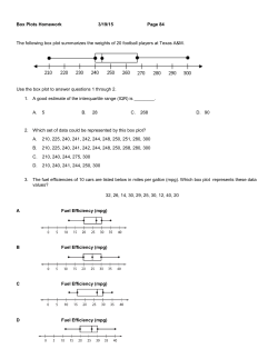
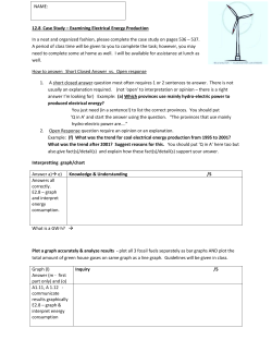


© Copyright 2026