ABC
docz
Explore
Log in
Create new account
Download
Report
No category
The Latent Process Decomposition of cDNA Microarray Data Sets
How To Use Longitudinal Patient Data (LPD) Your Q&A Guide to
Document 10251
Development & Validation of Genomic Classifiers for Treatment Selection Richard Simon, D.Sc.
LRpath analysis reveals common pathways dysregulated via DNA methylation across cancer types
Analysis of Gene Expression Data Using BRB-Array Tools Richard Simon
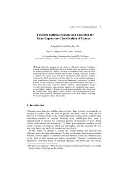
Towards Optimal Feature and Classifier for Gene Expression Classification of Cancer //// 1
Clinical Quiz Answers wers (See page 64) Part
Keynote Lectures Sunday, June 24th 8:15 AM – 9:30 AM
why men dIe earlIer and suffer more oCt. 9
review article Microarray Data analysis for Differential expression: a tutorial
*PROSTATE PROBLEMS? THE ALTERNATIVES THAT CAN HELP
letters A novel solenoid fold in the
© Copyright 2026
About abcdocz
DMCA / GDPR
Report