1. finance
2. investing
3. stocks

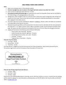
Milevsky and Salisbury (27 Feb 2004)
Globe and Mail Contest
Probabilistic Investing:
or
How to Win the Globe and Mail’s
Stock Picking Contest (50% of the time)1
By:
Moshe A. Milevsky, Ph.D.2
Finance Professor, York University
Executive Director, The IFID Centre
and
Thomas S. Salisbury, Ph.D.
Professor of Mathematics and Statistics, York University
Deputy Director, The Fields Institute
1. Introduction and Motivation:
For the past eight years the Globe and Mail newspaper has held an annual stock
picking contest entitled My One and Only. In this competition, which starts on January 1st
of each year, a variety of financial commentators, money managers and even academics
are asked to select one stock – from the universe of stocks trading above $1 – of any
public company quoted on the Toronto Stock Exchange (TSE). In addition to human
participants, a completely random selection is added to the competition as well. The
performance of all entries are tracked daily on a popular website and reported on
quarterly in the actual newspaper, but the winner of the contest is the sole individual with
the best performing stock at the end of the year, based on the close of trading on
December 31st. The final results of the contest are announced with much fanfare and
publicity on the front page of the Report on Business section in the first week of the
subsequent year. Aside from the publicity (negative or positive) from being part of the
game, the winner’s only reward is a coffee mug, compliments of the Globe and Mail.
1
This article is being prepared for submission to the Canadian Investment Review. Please do not quote or reference
without author’s permission. Revisions to this paper can be downloaded from www.ifid.ca .
2
The contact author (Moshe Milevsky) can be reached at Tel: (416) 736-2100 x 60014 or via Email at
[email protected]. Both author’s would like to acknowledge David Promislow for helpful comments and Josh
Landzberg for excellent research assistance compiling the stock-price data.
Page 1 of 21
Milevsky and Salisbury (27 Feb 2004)
Globe and Mail Contest
In 2002 and then again in 2003, a Professor of Finance at one of Canada’s leading
business schools (and one of the authors of this paper) won the contest by beating all
other participants, as well as the TSE market index by a wide margin. And, while it is easy
to dismiss such results as completely attributable to luck, there is in fact a well-developed
theory behind optimal behavior in such a contest. A rational and cognizant player can
substantially increase the odds of winning the investment contest by playing the game
optimally. We will review this theory in detail and make the interesting argument that
picking stocks to win an investment game is quite different from selecting securities for
personal investment portfolio.
In other words, motivated by this investment contest and the surrounding public
interest, our paper takes the opportunity to review the theory of stochastic games and
provide some anecdotal evidence as well as rigorous insights into the best way to win the
Globe and Mail’s stock picking contest. Our main intellectual objective, however, is to
illustrate the critical difference between a rational and prudent strategy for building wealth
versus the optimal strategy for picking stocks in these all-or-nothing contests. And, while
there are many such investment games in existence -- the oldest and most popular being
the Wall Street Journal’s quarterly analyst vs. dartboard contest – the national stature and
exposure of the G&M contest and the involvement of one of the authors makes this an
ideal case study.
The actual paper is organized as follows. Section 2 provides a gentle introduction to
the theory behind investment contests, and demonstrates that the strategy with the best
odds of winning is somewhat counter-intuitive. Namely, we demonstrate that one should
pick securities with very high idiosyncratic (i.e. diversifiable) risk, but with zero or possibly
negative beta; in the lingo of modern portfolio theory. This tactic is perfectly justified
despite over 40 years of dogma which preaches no equilibrium compensation for taking on
idiosyncratic risk in capital markets. Furthermore, we show that the a priori probability of
winning such a contest under our suggested optimal strategy comes close to, but can
never exceed, 50%. An unobtrusive technical appendix provides the necessary probability
theory. Section 3 of the paper reviews the actual stock selections and choices of the
Page 2 of 21
Milevsky and Salisbury (27 Feb 2004)
Globe and Mail Contest
contest participants over the 8 years of the contest. By examining betas and volatilities,
we show that most of the winning stocks -- or the stocks that had the highest probability
of winning a priori -- did in fact conform to the above selection criteria.
Aside from theoretical insights, the practical lessons from this paper’s analysis is
that picking stocks with the sole objective of winning a contest should not be viewed as a
proxy for providing any guidance on building a well-diversified investment portfolio.
Professional investment managers and individuals who manage their own portfolios must
understand and acknowledge the inherent statistical illusions induced by such games.
Indeed, one might go so far as to argue that the optimal strategies in both these
endeavors are orthogonal to each other. Ex post one might be tempted to ascribe talent to
winners, and especially repeat winners, when in fact the odds strongly favor such an
outcome by chance when the game is played optimally. Anyone who attempts to replicate
or mimic the behavior of the so-called contest winners with real money is likely to be
disappointed. The message is crystal clear. Do not try this at home.
2. What Does Theory Tell Us About Winning Investment Contests?
Modern investment theory – as originally developed by Harry Markowitz and Bill
Sharpe3 – argues that all stocks can be classified by a limited set of parameters, namely
their expected return and covariance structure. And, although a priori it would seem that
the optimal strategy for winning a contest is to locate the stock with the highest (best)
expected return, the truth is far from being that simple. In fact, given the difficulty in
estimating expected returns over very-short periods of time, the secret to winning such a
contest (or at least maximizing the odds) is to completely ignore expected returns and
focus exclusively on the covariance of the stock in question.
Traditional mean-variance framework underlies most of today’s professional money
management and is the springboard for our analysis. The technical appendix provides a
detailed derivation of the probability of winning as a function of the expected return,
3
We refer the interested reader to the book by Elton and Gruber (1995), and especially chapter 7, for a detailed
discussion of modern portfolio theory and specifically the mathematics underlying mean-variance analysis.
Page 3 of 21
Milevsky and Salisbury (27 Feb 2004)
Globe and Mail Contest
standard deviation and correlation structure. This analytic machinery can be used to
demonstrate that for any reasonable expectation of investment returns – which we argue
is almost impossible to estimate over short contest horizons – the probability of winning is
most sensitive to the covariance structure of the security. The secret to winning – if there
is any secret – is to pick a stock that is highly volatile and negatively correlated to the rest
of the pack. This implicitly maximizes the odds of an extreme ranking. When done
properly, the extreme ranking which is induced by this strategy will result in either winning
the contest (50%) or coming dead last (50%). And since true money is never at play in
these games, a 50/50 chance is the best one can hope for. Recall that in contrast to real
life where the difference between 3rd or 4th or 5th place represents real dollars and cents in
one’s retirement portfolio or quarterly evaluation, there is little difference for those placing
anything other than 1st. Though, for a real money manager, as opposed to a finance
professor, it might be argued that some utility is derived from finishing in the top half of
players, even if one doesn’t finish first. And, while some might argue the harm caused by
a last place or similar finish, these risk-averse contestants have the option of simply not
participating. In the language of decision theory, the objective of the contest is to
maximize a binary utility function which either takes on the value of one (winning) or zero
(not winning). This is quite different from utility functions which balance risk – a.k.a
shortfall, standard deviation or regret – and expected returns. Maximizing a smooth and
differentiable utility function leads to a diversified portfolio of individual stocks, as
originally shown by Markowitz. A binary objective function induces a strategy which
maximizes the probability of beating a stochastic benchmark, independently of the
magnitude of loss or disappointment.
4
To understand the counter-intuitive implications of this strategy and the impact of
volatility and correlation on winning, we offer the following simplistic example. Assume we
are asked to participate in a contest with only two other participants, each of whom has
already selected their stock. We denote the standard deviation (or volatility) of our
4
We refer the interested reader to the recent papers by Brown, Harlow and Starks (1996), Chevalier and Ellison (1997)
as well as Busse (2001) or Goetsmann, Ingersoll and Ross (2003) for a theoretical discussion and some empirical
evidence on the impact of financial incentives on professional portfolio managers in a tournament-like environment.
Indeed, it appears that similar game-theoretic behavior and strategies might be optimal in the money management
business.
Page 4 of 21
Milevsky and Salisbury (27 Feb 2004)
Globe and Mail Contest
competitors’ stocks by the symbols { σ 1 , σ 2 } and their mutual correlations by the symbol
{ ρ12 }. Recall that volatility is a proxy for the range of possible values for the end-of-year
investment returns, while correlation measures the extent to which the two move
together. Correlation values range from { − 1 ≤ ρ ≤ 1 }. Volatility can be as low as zero, for a
risk-free product and can goes as high as infinity, in theory.
We are now asked to join the contest – knowing our competitors’ two picks – and
must select a stock that is characterized by a standard deviation { σ 3 } and a correlation
pair { ρ 31 , ρ 32 }. For the purpose of this example, we limit our search amongst the universe
of correlation pairs that are equal. In other words, we assume that ρ 32 = ρ 31 = ρ . The
same idea would apply under a more complicated search. Figure #1 is a graphical
illustration of the triangular relationship between our yet-to-be-made stock pick and our
two competitors’. If, instead of 2 competitors we had 7, then Figure #1 would have a
pyramid-like structure (in 7 dimensions) displaying all the possible correlations. While this
all might appear somewhat abstract and removed from the process of stock picking – after
all, where is the discussion of price-to-earning ratios, dividends or growth rates? – we
believe this framework truly captures the essence of the competition.
Competitor #1
σ1
ρ
Figure #1
Competitor #2
σ2
ρ12 = ρ21
ρ
Our Pick
σ3
With this model in hand, Table #1 provides a number of important insights into the
optimal strategy for winning the contest, which differs markedly with best practices for
portfolio construction. If we select a stock that is completely uncorrelated ( ρ = 0 ) with our
Page 5 of 21
Milevsky and Salisbury (27 Feb 2004)
Globe and Mail Contest
competitors’ stock picks and all contestants have the same investment volatility ( σ = 1 ),
the table illustrates that the probability that we win the contest is exactly 1/3. This should
be intuitive. There are three (2+1) stocks in the contest, they are all identical and
symmetric, and therefore all have an equal chance of winning. The same 1/n probability
would apply for n symmetric securities as well. For those readers interested in a rigorous
proof, we refer them to equation (eq.7) in the appendix which must be generalized to R n .
Table #1: Probability of Winning as a Function of Selected Correlation and Volatility
Our Two Opponents Select Equally Volatile ( σ 1 = σ 2 ), But Uncorrelated ( ρ12 = 0 ) Stocks.
Correlation
σ 3 = 0.5
σ 3 = 1.0
σ 3 = 2.0
σ 3 = 5.0
σ 3 = 10.0
ρ = +0.7
9.7%
13.4%
34.2%
44.8%
47.5%
ρ = +0.5
19.6%
24.9%
36.6%
45.1%
47.6%
ρ = 0.0
28.2%
33.3%
39.8%
45.6%
47.7%
ρ = −0.50
32.0%
36.6%
41.4%
45.9%
47.8%
ρ = −0.70
33.1%
37.5%
41.9%
46.1%
47.9%
In contrast to the symmetric 1/n result, when our competitors’ correlations are zero
( ρ12 = 0 ) and we select a stock that is twice as volatile as our competitors’ ( σ = 2 ), the
probability of winning the contest goes from 33.3% to 39.8%. When our standard
deviation is increased by a factor of ten ( σ = 10 ), the probability of winning then jumps to
47.7% In fact, one can show that as the standard deviation goes infinity, the probability of
winning converges to exactly 50%. This is true regardless of the number of stocks in the
contest. For example, if there are 8 stocks in the contest, the neutral symmetric
probability of winning is 1/8 which is 12.5%. Increasing the volatility of the stock will
rapidly drive our probability of winning to 50%, leaving the other 50% chance to be
shared amongst our 7 competitors. Note that we are focusing on total volatility, which is
the sum of both systematic (non diversifiable) and non-systematic (diversifiable) risk.
If we decrease the correlation ( ρ << 0 ) between our pick and our competitors’
picks, the probability of winning increases to the same 50% upper limit, but at a much
Page 6 of 21
Milevsky and Salisbury (27 Feb 2004)
Globe and Mail Contest
higher rate. Indeed, when the correlation between our selection and the two other picks is
set to minus 70% ( ρ = −0.70 ), the probability of winning increases to 37.5% (from
33.3%) when the volatilities are identical. Note that we have restricted the correlation
parameters in Table #1 to the range {-0.7, +0.7} so as to maintain an appropriate
covariance matrix that is positive semi-definite. We refer the interested reader to the
appendix where this is explained in greater detail.
In the opposite volatility direction, if our stock pick is half as volatile as our two
competitors’ ( σ = 0.5 ), the probability of winning the contest is greatly reduced. In fact,
when our correlation to our competitors’ is set to a positive 70% value, our probability of
winning drops to a mere 9.7% compared to the equal chances under a completely
symmetric contest. In this case, i.e. when we are 70% positively correlated to both our
competitors’, but half as volatile, the remaining 100% - 9.7% = 93.3% percent of winning
is split evenly between the two opponents, for an equal 46.65% chance of winning. Thus,
a poor choice of either correlation of volatility on our end not only harms our chances of
winning, but obviously greatly enhances our opponents’ positions. Clearly, there is a
substantial amount of game theoretical implication when this contest is played by rational
investors, each fully cognizant of their opponents’ rationality. A full analysis of the relevant
game theory is beyond the scope of this article, and we refer the interested and brave
reader to a series of papers by Browne (1999, 2000) for more information about
maximizing the probability of beating the return from a given portfolio of stocks within a
game-theoretic context. Our point here is to emphasize the impact of volatility above all.
Table #2: Probability of Winning as a Function of Selected Correlation and Volatility
Opponents Select Equally Volatile ( σ 1 = σ 2 ), but -25% Correlated ( ρ12 = −0.25 ) Stocks
Correlation
σ 3 = 0.5
σ 3 = 1.0
σ 3 = 2.0
σ 3 = 5.0
σ 3 = 10.0
ρ = +0.60
6.28%
15.5%
33.6%
44.4%
47.3%
ρ = 0.00
25.0%
31.2%
38.4%
45.0%
47.4%
ρ = −0.20
27.2%
32.9%
39.3%
45.2%
47.5%
Page 7 of 21
Milevsky and Salisbury (27 Feb 2004)
Globe and Mail Contest
Table #2 provides information similar to Table #1, except that we assume the
correlation between our opponents’ stock picks is negative 25%, albeit with equal
volatility. Once again our probability of winning the contest depends on our stock’s
volatility { σ 3 } as well as the correlation with the other two stocks.
The most pertinent observation is that the probability of winning when our
opponents have selected anti-correlated stocks is reduced at all levels of volatility. For
example, in contrast to Table #1, if we select zero correlation with our opponents’
( ρ = ρ 31 = ρ 32 ), and we have all picked stocks with equal volatility, our probability of
winning is reduced from 33.3% in Table #1 to 31.2% in Table #2. This might not seem
like much of a change, but as we increase the number of contestants, the relative gap will
become larger and more noticeable. It is important to note that the relationship between
winning and correlation does not appear to be universally monotonic, even though the
probability of winning does increase with reduced correlation in both Table #1 and Table
#2. At extreme levels of opponents’ correlations, there might be a reduced benefit to
selecting even more negatively correlated stocks.
One thing is true regardless of all the other parameters in the system, the greater
our stock’s volatility, the greater our chances of winning. Once again, the intuition for this
fact is as follows. When selecting an extremely volatile stock there are two possible
outcomes: either our stock earns a very high (extremely positive) return, or we earn a
very low (i.e. extremely negative) return. The odds of either outcome are roughly 50/50.
If we achieve a favorable return and our overall correlation with our opponents’ is
negative, they will likely experience a worse relative to the mean, and we win (50%
chance). This is why both high volatility and negative correlation is important. The first
factor places us in the required extremes while the second factor places our opponents on
the other side.
2.1 Unknown Opponents, the Connection to Beta and Diversifiable Risk
One of the issues that arises when implementing such a strategy in practice, is that
we are unlikely to be told in advance the name (and hence the historical volatility and
Page 8 of 21
Milevsky and Salisbury (27 Feb 2004)
Globe and Mail Contest
correlation) of our opponent’s stock. However, if we assume they will be selected
randomly from the available market -- and we obviously have to compete against the
market index as a whole -- then we can focus on two hypothetical opponents. The first is
the market itself, and the second is a stock with some unknown beta relative to the
market.
Recall that modern portfolio theory dictates that diversifiable (i.e. idiosyncratic)
investment risk is not worth bearing since it is not compensated in economic equilibrium5.
Under this theory, the only risk that matters is systematic, and the expected return from
any security is linearly related to its beta. The greater the beta -- which is the covariance
of the security’s return with the general market portfolio, scaled by the variance of the
security -- the greater is the expect return. Thus, investors who are interested in
maximizing expected returns without any concern for risk would optimally select securities
with the highest beta. The mathematical definition of beta is:
βi =
Cov( X i , X m ) ρ imσ i
=
.
Var ( X m )
σm
From a mathematical point of view, the beta of the stock is a function of three ingredients,
we discussed earlier in our analysis, the correlation with the market portfolio, the standard
deviation of the stock in question and the standard deviation of the market portfolio.
Now, as we argued above, the optimal strategy in a contest with a zero-one payoff
function is to locate a security with a negative correlation { ρ im } to our competitors’ (i.e.
the market), and with as high a volatility { σ i } as possible. Thus, the optimal strategy is to
pick very volatile and possibly negative beta stocks. This, once again, is in stark contrast
to the objectives of any portfolio or wealth manager who is interested in maximizing
expected returns subject to some reasonable constraints on risk.
The theory is unambiguous in recommending a very risky strategy to maximize the
probability of winning the contest. Indeed, whether the equilibrium expected return from
the stock is 5%, 15% or even 20%, the covariance matrix will play a far larger role in the
outcome of this, or in any contest for that matter. We now move on to examine the
5
See the recent paper by Goyal and Santa-Clara (2003) for recent empirical evidence that perhaps some idiosyncratic
risk might be worth bearing.
Page 9 of 21
Milevsky and Salisbury (27 Feb 2004)
Globe and Mail Contest
mechanics and actual choices made participants in the Globe and Mail contest during the
past 8 years.
3. Which Stocks Did Contestants Actually Choose?
As we explained in the introduction, the contest operates in the following manner.
In late December of each year the investment editor of the Report on Business tabulates
the performance of the previous year’s contestants and asks the top 4 or 5 to participate
in the coming year’s event and select another stock. In addition, the editor picks 4 or 5
other contestants (at random) from a broad range of practitioners and academics in
Canada. This assures a reasonable amount of turnover in the pool of contestants (unless
one of them continues winning.) Occasionally contestants decide not to participate in the
following year’s contest and voluntarily withdraw, even though they earned a top berth in
the previous year. Each contestant must select a stock amongst all securities traded on
the Toronto Stock Exchange (TSE), valued at more than $1. To add an element of humor,
the editors select a young child from the Globe and Mail’s extended family and ask them to
randomly toss a toy at the stock quote pages. This becomes yet another contestant6. In
the first year of the contest (1997) there were a total of 8 participants, the list was
expanded to 9 for the period 1998 – 2003, and last year the total came to 10. Another
complication that has only recently been added is the option to ‘cash in’ at the end of each
quarter. And, while this option has never been exercised by any of the participants, it is
quite conceivable that a large enough return in any given quarter might induce a
participant to take the money off the table and cash-out. This further complicates the
optimal strategy since one must now decide if and when to cash in, but this will not
reverse our main conclusion about the optimality of high volatility and/or negative beta
strategies.
Tables 3a and 3b display the selections made by all participants during the past 8
years, together with the standard deviation (volatility) and betas of the selected stock
which we have computed using textbook methods. The stocks are listed in the order of
6
In fact, in the year 2000 the winner of the contest was a windup toy Santa who enviously picked the company Denbury
Resources and earned a total return of 179% during the year.
Page 10 of 21
Milevsky and Salisbury (27 Feb 2004)
Globe and Mail Contest
their final ranking and return. Not surprisingly, the winning stocks always outperformed
the S&P/TSX market by a very wide margin, even in years when the market as a whole
dropped in value. In most years the winning stock earned well in excess of 100% return.
Page 11 of 21
Milevsky and Salisbury (27 Feb 2004)
1997 Contestants
Patrick McKeough
Irwin Michael
Steven Misener
David Bissett
Robert Millham
Robert Boaz
Ron Meisels
Josef Schachter
1998 Contestants
Colleen Moorehead
Patrick McKeogh
David Bissett
Nebby The Cat
Steven Misener
Sebastian van Berkom
Irwin Michael
Benj Gallander
Ian Ihnatowycz
1999 Contestants
Steven Misener
David Bissett
David Driscoll
Patrick McKeough
Suzann Pennington
Duncan Stewart
Hannah Willis
Norman Raschkowan
Colleen Moorehead
2000 Contestants
Clockwork Santa
Patrick McKeough
Derek Webb
Moshe Milevsky
Ian Joseph
Steven Misener
David Driscoll
David Bissett
Richard Croft
Globe and Mail Contest
Stock Pick
Corporate Foods
Canadian Occidental Petroleum
Eurogas
Foremost Industries
Hummingbird Communications
Carmanah Resources
S&P/TSX Index
Stampeder Exploration
Golden Rule Resources
Ticker
CFL
CXY
EUG
FMO
HUM
CKM
Stock Pick
ATI Technologies
Nova Corp.
Tecsyn International
Pet Valu
Tembec
S&P/TSX Index
Hummingbird
Alliance Forest
Breakwater
American Eco
Ticker
ATY
NCX
TSN
PVC
TBC
Stock Pick
BCE Emergis
Axia Netmedia
Patheon
Toronto-Dominion Bank
S&P/TSX Index
Sobeys
Mortice Kern Systems
Economic Investment Trust
RealFund (Riocan REIT)
Newbridge Networks
Ticker
IFM
AXX
PTI
TD
Stock Pick
Denbury Resources
CAE
BCE
Investors Group
TD Bank
S&P/TSX Index
Int. Forest
Maax
Glendale Int.
Bid.com Int.
Ticker
DNR
CAE
BCE
IGI
TD
SDX
GNU
HUM
ALP
BWR
ECX
SBY
MKX
EVT
RFNU
NN
IFP.A
MXA
GIN
BII
% Return
81.5%
48.0%
32.0%
30.0%
16.5%
11.0%
9.7%
5.3%
-86.6%
Beta
1.09
N/A
-0.47
N/A
0.28
0.77
1.00
1.34
1.06
Volatility
18.3%
N/A
66.9%
N/A
43.4%
35.4%
11.6%
33.4%
78.7%
% Return
110.9%
47.1%
16.7%
10.2%
7.7%
0.4%
-34.6%
-37.7%
-76.8%
-82.8%
Beta
-0.55
-0.05
-0.78
0.66
0.71
1.00
-0.76
0.01
-1.80
1.36
Volatility
29.3%
20.6%
53.2%
23.6%
38.9%
15.0%
47.8%
39.2%
86.9%
57.4%
% Return
459.6%
249.1%
112.9%
47.4%
26.0%
18.8%
17.0%
-4.2%
-8.0%
-30.2%
Beta
0.37
-0.61
0.21
0.43
1.00
-0.29
0.05
0.01
1.11
N/A
Volatility
85.4%
84.6%
48.5%
48.7%
28.8%
18.5%
60.2%
34.0%
40.1%
N/A
% Return
179.2%
146.5%
34.8%
26.2%
12.1%
9.9%
-1.3%
-23.6%
-70.2%
N/A
Beta
-1.56
-0.11
-0.04
-0.31
-0.10
1.00
-0.44
0.01
0.41
N/A
Volatility
45.4%
23.6%
37.7%
27.2%
37.0%
15.7%
53.5%
17.9%
58.1%
N/A
Table 3a: Stocks Selected by Contest Participants, Their Volatility and Final Return.
Page 12 of 21
Milevsky and Salisbury (27 Feb 2004)
2001 Contestants
Veronika Hirsch
Steven Misener
Moshe Milevsky
Sharon Ranson
Jane the orangutan
Patrick McKeough
Globe and Mail Contest
Stock Pick
Gulf Canada Resources
Interpape Polymer Group
Industral-Alliance Life
TD Bank
Thomson
BCE
S&P/TSX Index
Mosaid Technologies
Nortel
Ensign Resource
Ticker
GOU
ITP
IAG
TD
TOC
BCE
Stock Pick
Ketch Energy
Royal Bank of Canada
E-L Financial Corp.
AUR Resources
Magna Int'l
S&P/TSX Index
Quebecor Inc.
Labopharm Inc.
Slater Steel
GT Group Telecom
Ticker
KCH
RY
ELF
AUR
MG.A
Ticker
SNG
ELD
WJA
ABZ
Madeleine Northfield
Sharon Ranson
Janis Mackey Frayer
Ron Meisels
Nick Majendle
Stock Pick
Canadian Superior Energy
Eldorado Gold Corp.
WestJet Airlines
Aber Diamond Corp.
S&P/TSX Index
Manulife Financial
Sun Life Financial
Bombardier Inc.
Aecon Group Inc.
Stelco Inc.
2004 Contestants
Rachel Willis
Moshe Milevsky
David Skarica
Lesley Scorgie
Veronika Hirsch
Marco Den Ouden
Yola Edwards
Michael Smedley
Vincent Delisle
Amanda Lang
Stock Pick
Husky Injection Molding Systems
Forbes Medi-Tech Inc.
Tan Range Exploration Corp.
Westjet Airlines Ltd.
GMP Capital Corp.
Peyto Energy Trust
QLT Inc.
TSX Group Inc.
Killam Properties Inc.
Biovail Corp.
Andrew McCreath
Ian Joseph
Rohit Sehgal
2002 Contestants
Moshe Milevsky
Sharon Ranson
Steven Misener
Ron Meisels
Veronika Hirsch
Buzz Lightyear
Philip Strathy
Fabrice Taylor
Malvin Spooner
2003 Contestants
Moshe Milevsky
David Skarica
Leslie Scorgie
Veronika Hirsch
% Return
61.6%
20.5%
14.8%
-5.5%
-15.8%
-16.8%
-18.0%
-60.2%
-75.3%
-75.9%
Beta
0.39
0.59
0.14
-0.18
0.35
0.04
1.00
1.29
0.85
1.08
Volatility
42.7%
95.1%
21.7%
28.7%
37.6%
19.3%
21.9%
110.8%
60.3%
45.1%
% Return
108.3%
11.6%
8.7%
-2.4%
-12.9%
-14.1%
-26.6%
-67.4%
-69.8%
-100.0%
Beta
0.63
0.01
0.60
0.68
0.23
1.00
-0.71
-0.56
-0.28
-0.96
Volatility
69.0%
20.0%
28.9%
43.5%
21.8%
21.2%
49.9%
69.1%
40.9%
166.1%
MFC
SLF
BBD.B
ARE
STE.A
% Return
117.3%
95.7%
76.2%
52.9%
29.7%
21.2%
20.2%
2.4%
-4.2%
-35.0%
Beta
-2.00
0.29
2.37
0.02
1.00
0.29
0.18
-1.24
0.18
0.99
Volatility
102.4%
76.0%
57.7%
27.2%
13.9%
26.8%
25.1%
39.9%
34.8%
47.4%
Ticker
HKY
FMI
TNX
WJA
GMP
PEY
QLT
X
KMP
BVF
% Return
?
?
?
?
?
?
?
?
?
?
Beta
2.17
0.81
0.57
1.78
N/A
1.49
-0.24
N/A
-1.66
-1.25
Volatility
43.5%
97.1%
53.8%
35.0%
N/A
24.1%
49.9%
N/A
60.5%
69.7%
MSD
NT
ESI
QBR
DDS
SSI
GTG.B
Table 3b: Stocks Selected by Contest Participants, Their Volatility and Final Return.
Page 13 of 21
Milevsky and Salisbury (27 Feb 2004)
Globe and Mail Contest
Notes to Table 3a, 3b: The Betas and volatilities in this table are calculated based on 12 months of
historical returns prior to the start of the contest. For example, for Gulf Canada Resources, which was
selected for the 2001 year contest, the beta and volatility figures are calculated based on year 2000 returns.
However, calculations for AXX and SBI (1999 Contest) are based on 1999 returns, and calculations for IAG
(2001 Contest) are based on 2001 returns. These exceptions are due to the lack of a complete set of data
for the prior years, likely because of demutualizations or IPO’s. Additionally, where “N/A” is stated in the
table, it is due to a lack of stock-price data.
The common and erroneous perception from a casual examination of these tables is
that financial experts -- or at least the participants in these contests -- are able to select
winning stocks that consistently beat the market and earn handsome returns. Indeed,
quite a few of the winners have marketed their success in this contest as evidence of their
stock picking prowess. Some winners have added this achievement to their public
biography and CVs. Yet, as we have argued in the previous section, perceptions vis a vis
optimal contest strategies are from the harsh reality of picking a well diversified portfolio
of stocks that earns positive risk-adjusted returns in the long-run.
In the 1997 contest the winning stock (CFL) had a volatility of only 18% and a beta
close to one which would appear to negate our theoretical claims that a highly volatility
and/or negative beta security is required to win the contest. However, note that our model
only provides stochastic predictions and there is always a chance that thee coin comes up
“tails”. More importantly, the losing stock in the 1997 contest (GNU) actually had the
highest volatility of 78.7% which is consistent with our theory - namely that a high
volatility stock provides the best odds of coming in first, or last. If the stock does not win,
it is quite likely to be the worst performer. The high volatility places the probable
outcomes on the extreme of the distribution and therefore one of two possible events
occur. In 1998, once again, the highest volatility stock did not win the contest, but its
(ATY)’s beta was in fact negative. More importantly, the two losing stocks (BWR and ECX)
had the highest volatility of 86.9% and 57.4% respectively. Once again, volatility placed
the outcome in the extremes. We emphasize, from a methodological point of view, that
our volatility and beta was estimated using 12 months of data prior to the contest. Thus,
the volatility of BWR and ECX in 1997 – on the eve of the 1998 contest – was 86.9% and
Page 14 of 21
Milevsky and Salisbury (27 Feb 2004)
Globe and Mail Contest
57.4%. In fact, despite coming in dead last, they were both rational choices and excellent
candidates to win such a contest.
In 1999, the winning stock (IFM) earned an astounding 459% return over the 12
months and was classified with a volatility (in 1998) of 85.4%. This volatility was the
highest amongst the stocks selected for the 1999 contest, and in fact is precisely what
theory would predict. The highest volatility (and low beta) stock placed first. In the year
2000, once again, theory was vindicated with DNR winning the contest and having a
volatility much higher than the market, as well as the most negative beta amongst the
stocks selected that year. Note that information about bid.com, the worst stock, was
unavailable. This is likely due to its having ceased trading during the year which is yet
another example of high volatility leading to extreme outcomes. In the year 2002, once
again, the highest volatilities were at the extremes, and in the year 2003 the highest
volatility and lowest (negative) beta placed first. As pointed out in the introduction, the
winning stocks in 2003 (SNG) and in 2002 (KCH) were selected by the same individual,
using a variant of the theoretical strategy described in the previous section. Of course, at
the present time, the jury is still out on the winner for 2004, but FMI – the 2002 and 2003
winner’s pick – is the highest volatility stock at 97.1%, albeit the beta is positive. But recall
from Table #1 that the sigma effect is stronger than the correlation effect which is why it
might make sense in practice to select a higher volatility even at the expense of a positive
beta.
In sum, consistent with our theoretical arguments, it seems that the most volatile
and negatively correlated (or at least low beta) stocks were amongst the winning (or
extreme losing) circle in any given year.
4. Conclusion and Implications for Portfolio Management
Portfolio selection and wealth management is about good stock picking as well as
balancing risk and return. But, in the context of investment contests, these qualities have
little bearing on the outcome. And, though at first glance it might appear that maximizing
Page 15 of 21
Milevsky and Salisbury (27 Feb 2004)
Globe and Mail Contest
the probability of winning may seem like a reasonable and innocuous investment strategy7
to apply in one’s daily life, a deeper examination reveals its flaws. Interestingly, if the
contest would require each contestant to select two stocks – and their returns were
averaged – a large part of this perverse incentive would be eliminated.
The implications of our analysis go far beyond the strategies required to win a
popular game. Anecdotal evidence suggests that individual investors observe and then
mimic the selections made by so-called expert participants in such contests. In fact,
although our sample is statistically small, we found that the average daily volume – on the
Monday following the announcement in the G&M -- for the stocks selected by the previous
year’s winner, was 5 to 10 times the normal amount. These effects are consistent with an
extensive and growing branch of research in the field of behavioral finance – see Odean
and Barber (2003) or Rashes (2001) -- which documents persistent biases, mistakes and
consumer susceptibility to noisy signals. It is therefore extremely important that
professional fund managers, as well as the press who are involved in promoting and
participating in these contests, emphasize the hazards of mimicking these stock picks with
one’s own investment portfolio.
Epilogue
As of the close of trading at the end of February 2004, Forbes Medi-Tech (stock
symbol FMI) – which was selected in early 2004 as this year’s pick by the 2002 and 2003
champion – has increased in value by more than 140% in the first two months of the year.
The nearest competitor, Killiam Properties Inc. (KMP), has increased in value by 30%. If
indeed this relative ranking is maintained for the remainder of the year, the G&M will have
crowned an unheard of three-time winner. Yet, using the optimal strategy described in the
paper, the chances of a three-peat performance is a mere (1/2)^3 = 1/8, which is close to
92 times greater than a naïve (1/9)^3 = 1/729 and much less impressive than the press
(or the winner) would be willing to admit.
7
In fact, this strategy has been advocated on the portfolio level as a method of saving for retirement (i.e. maximize the
probability of having a fixed dollar amount at age 65) by a number of authors, including Ho, Milevsky and Robinson
(1996) in the pages of the Canadian Investment Review.
Page 16 of 21
Milevsky and Salisbury (27 Feb 2004)
Globe and Mail Contest
Technical Appendix
In this appendix we briefly summarize the analytics behind the probability of
winning when there are a total of (2+1) competitors in the contest; two opponents plus
ourselves. The computations can be generalized from 3 to n stocks by scaling-up the
integral described below. We start by denoting the stock picks of our two competitors by
the symbols S1 ( µ1 , σ 1 , ρ12 ) and S 2 ( µ 2 , σ 2 , ρ 21 ) , where each stock is assumed to obey a
LogNormal distribution (a.k.a. geometric Brownian motion) and parameterized by an
expected return (drift), standard deviation (volatility), and correlation ( ρ12 = ρ 21 ) with the
other security. These are standard assumptions in financial theory and underlie the
foundations of the Capital Asset Pricing Model (CAPM). At this point, our model is
obviously predicated on actually knowing our opponents’ selections. In the body of the
paper we discuss what to do when this knowledge is unavailable. Also, when dealing with
n securities instead of (2+1), each stock would be characterized by its relation to all other
stocks, via a covariance matrix.
We must now select a third stock, denoted by S 3 ( µ 3 , σ 3 , ρ 31 , ρ 32 ) , with the highest
~
probability of beating the stocks selected by our two opponents. If we let S i , i = 1,2,3
denote the random price of each of these stocks at the end of the contest (i.e. year-end)
~
and then define X i = ln[ S i / S i ], i = 1,2,3 to be the continuously compounded return, our
problem boils down to computing the following:
w := Pr[ X 3 > max[ X 1 , X 2 ]] .
(eq.1)
The variable (stock’s investment return) X 3 will win the contest if and only if it beats the
maximum of the two investment returns generated by the competitors. Note that by
computing and working with logarithms of the actual stock price, we are transformed from
a LogNormal environment into a world of normality. Of independent interest is the
quantity R * = E[max[ X 1 , X 2 , X 3 ]] , which is the investment return earned by the winner of
the contest. It is relatively easy to show that R * > max[ µ1 , µ 2 , µ 3 ] .
Page 17 of 21
Milevsky and Salisbury (27 Feb 2004)
Globe and Mail Contest
A multi-variate normal random variable is defined and characterized by its expected
return and covariance matrix. Formally, let:
⎛ σ 1σ 1
⎜
C := ⎜ ρ 21σ 2σ 1
⎜ρ σ σ
⎝ 31 3 1
ρ12σ 1σ 2
σ 2σ 2
ρ 32σ 3σ 2
ρ13σ 1σ 3 ⎞
⎟
ρ 23σ 2σ 3 ⎟ ,
σ 3σ 3 ⎟⎠
(eq.2)
where C[i, j ] denotes the entry in the i’th row and j’th column of the covariance matrix.
Note, of course, that { ρ 23 = ρ 32 , ρ13 = ρ 31 , ρ 21 = ρ12 } and the distinct notation in equation
(eq.2) is used for cosmetic purposes only. We now define the inverse covariance matrix
IC := inv(C) , and follow the same convention for the individual terms IC[i, j ] . Also, we
let D := IC , which is the determinant of the inverse of the covariance matrix. It is
relatively straightforward to confirm this in our 3-asset case
D = −(σ 1 σ 2 σ 3 ( ρ 23 + ρ12 + ρ13 − 2 ρ12 ρ13 ρ 23 − 1)) −1 .
2
2
2
2
2
2
(eq.3)
Recall that the need for a positive semi-definite covariance matrix C imposes the algebraic
condition of D > 0 which then translates into an admissible range of correlation values for
the set {ρ 31 , ρ 32 } . For example, when the standard deviations are all arbitrarily set
to: σ i = 1, i = 1,2,3 , and the correlation between the competitors’ stocks is set to ρ12 = 0 , the
determinant is D = 1 /(2 ρ 2 − 1) , from equation (eq.3), and the positive semi-definite
condition imposed on the selected correlation collapses to the region {−1 / 2 < ρ < 1 / 2 }
when ρ := ρ 31 = ρ 32 . Thus, caution is warranted when ‘solving’ for the best parameters that
blindly maximize the probability of winning in equation (eq.1), since they may
inadvertently fall in a region that is unacceptable from a covariance matrix perspective.
Finally, we define the function:
Q ( x1 , x2 , x3 | µ1 , µ2 , µ2 ,σ 1 ,σ 2 ,σ 3 , ρ12 , ρ 31 , ρ 32 )
3
3
= ∑∑ ( xi − µi ) IC[i, j ]( x j − µ j )
(eq.4)
i =1 j =1
Equation (eq.4) is the usual quadratic form which is the basis of the ubiquitous normal
distribution. Thus, for example, when all three correlations { ρ ij } and expected return { µi }
Page 18 of 21
Milevsky and Salisbury (27 Feb 2004)
Globe and Mail Contest
parameters are set equal to zero and all three standard deviations { σ i } are set equal to
one, equation (eq.4) collapses to: Q ( x1 , x2 x3 ) = x1 + x2 + x3 .
2
2
3
With this notation in hand, the tri-variate probability density function (pdf) for the
normal distribution can be written as:
f ( x1 , x2 , x3 ) =
D
(2π )
3/ 2
⎫
⎧ 1
exp ⎨− Q ( x1 , x2 , x3 ) ⎬ ,
2
⎭
⎩
(eq.5)
where the function Q ( x1 , x2 , x3 ) in the exponent suppresses the parameters for notational
simplicity. The probability the random return { X 3 } will beat the better of the two random
returns { X 1 , X 2 } can be computed by integrating the pdf in equation (eq.5) over the
region in which x3 > max[ x1 , x2 ] , which can be expressed in integral form as:
∞ ∞
w=
∞
∫∫
−∞ −∞
∫ f ( x , x , x )dx dx dx
1
2
3
3
1
2
.
(eq.6)
max[ x1 , x 2 ]
Finally, using geometric arguments and visualizing the region of interest in R 3 , the
probability of winning the contest, w, can be re-written as:
w=
∞ x2
∞
∫ ∫ ∫
− ∞ − ∞ x2
∞ ∞ ∞
f ( x1 , x2 , x3 )dx3dx1dx2 + ∫
∫ ∫ f ( x , x , x )dx dx dx
1
2
3
3
1
2
(eq.7)
− ∞ x 2 x1
Equation (eq.7) is the basis of the calculations described in the body of the paper.
It can be used in a number of interesting ways. First, assuming a pre-determined set of
parameters – estimated using historical performance data -- for the opponents’ selections
{ µ1 , µ2 , σ 1 , σ 2 , ρ12 }, we can solve for the optimum combination of { µ3 ,σ 3 , ρ 31 , ρ 32 } which
maximizes w in equation (eq.7), taking into account the restriction imposed by D > 0 and
possibly some (realistic) limits on µ3 . We can then search amongst the available securities
in the market (TSX, contest) that exhibit statistical behavior closest to the optimum
parameters. Alternatively, we can start by estimating the { µ3 ,σ 3 , ρ 31 , ρ 32 } parameters for
each and every available security in the market, and then ‘plugging’ each estimated set
into equation (eq.7) and then finally picking the stock (i.e. parameter set) with the highest
integral value (i.e. the probability of winning.) Of course, in a contest with more than
(2+1) participants, the bounds of integration, as well as the precise integrand in equation
Page 19 of 21
Milevsky and Salisbury (27 Feb 2004)
Globe and Mail Contest
(eq.7) will have to be modified accordingly. In practice, for those who are interested in
implementing this procedure in higher dimensions, we recommend using a symbolic
computational language such as Maple – see Monagan, Geddes, Labahan and Vorkoetter
(1996) for a description of the software -- which is what we used to evaluate equation
(eq.7).
Note that in the actual paper we have assumed the mean return parameters
{ µ1 , µ 2 , µ3 } are all set to zero, thus our methodology remains agnostic about the ability to
estimate the expected return for any given security over the short length of the contest.
However, we stress that even if we were to arbitrarily plug-in a particular value for { µ }
into equation (eq.7), the volatility and correlation structure would have a much greater
influence on the probability of winning.
References:
Barber B.M. and T. Odean (2000), Trading Is Hazardous to Your Wealth: The Common
Stock Investment Performance of Individual Investors, Journal of Finance, Vol. 55(2), pg.
773 -806.
Browne, S. (1999), The Risks and Rewards of Minimizing Shortfall Probability, Journal of
Portfolio Management, Vol. 25(4), pg. 76-85.
Browne, S. (2000), Stochastic Differential Portfolio Games, Advances in Applied Probability,
Vol. 37(1), pg. 126-147.
Brown, K., W. Harlow and L. Starks (1996), Of Tournaments and Temptations: An Analysis
of Managerial Incentives in the Mutual Fund Industry, Journal of Finance, Vol. 51(1), pg.
85-110.
Busse, J.A. (2001), Another Look at Mutual Fund Tournaments, Journal of Financial and
Quantitative Analysis, Vol. 36(1), pg. 53 – 73.
Page 20 of 21
Milevsky and Salisbury (27 Feb 2004)
Globe and Mail Contest
Chevalier, J. and G. Ellison (1997), Risk Taking By Mutual Funds as a Response to
Incentives, Journal of Political Economy, Vol. 105, pg. 1167 – 1200.
Elton, E.J. and M.J. Gruber (1995), Modern Portfolio Theory and Investment Analysis, 5th
Edition, John Wiley and Sons, New York
Elton, E.J., M.J. Gruber and C.R. Blake (2003), Incentive Fees and Mutual Funds, Journal
of Finance, Vol. 58(2), pg. 779 – 804.
Globe and Mail, Saturday January 4th, 2003 (page C1) and Saturday January 3rd, 2004
(page B20).
Goetzmann, W.N., J.E. Ingersoll and S.A. Ross (2003), High-Water Marks and Hedge Fund
Management Contracts, Journal of Finance, Vol. 58(4), pg. 1685 – 1717.
Graham, J.R. (1999), Herding Among Investment Newsletters: Theory and Evidence,
Journal of Finance, Vol. 54(1), pg. 237-268.
Goyal, A. and P. Santa-Clara (2003), Idiosyncratic Risk Matters!, Journal of Finance, Vol.
58(3), pg. 975 – 1008.
Ho, K., M.A. Milevsky and C. Robinson (1996) Risk-Adjusted Retirement, Canadian
Investment Review, Vol. 9(1), pg. 19-27
Monagan, M.B., K.O. Geddes, G. Labahn and S. Vorkoetter (1996), Maple V Programming
Guide, Springer Verlag, New York
Rashes, M.S. (2001), Massively Confused Investors Making Conspicuously Ignorant
Choices, Journal of Finance, Vol. 56(5), pg. 1911-1927
Page 21 of 21